A new gas cooling model for semi-analytic galaxy formation models

Abstract

Semi-analytic galaxy formation models are widely used to gain insight into the astrophysics of galaxy formation and in model testing, parameter space searching and mock catalogue building. In this work we present a new model for gas cooling in halos in semi-analytic models, which improves over previous cooling models in several ways. Our new treatment explicitly includes the evolution of the density profile of the hot gas driven by the growth of the dark matter halo and by the dynamical adjustment of the gaseous corona as gas cools down. The effect of the past cooling history on the current mass cooling rate is calculated more accurately, by doing an integral over the past history. The evolution of the hot gas angular momentum profile is explicitly followed, leading to a self-consistent and more detailed calculation of the angular momentum of the cooled down gas. This model predicts higher cooled down masses than the cooling models previously used in galform, closer to the predictions of the cooling models in l-galaxies and morgana, even though those models are formulated differently. It also predicts cooled down angular momenta that are higher than in previous galform cooling models, but generally lower than the predictions of l-galaxies and morgana. When used in a full galaxy formation model, this cooling model improves the predictions for early-type galaxy sizes in galform.

1 Introduction

Understanding galaxy formation is a central aim of astrophysics. Galaxies are interesting objects in their own right. In addition, they are a tracer of the large-scale matter distribution, which is important for the study of cosmology, and also provide the background environment for astrophysical processes happening on small scales, such as star formation and black hole growth. Despite its importance, many aspects of galaxy formation remain poorly understood, because of the complexities of the physical processes involved.

Currently there are two major theoretical approaches to studying galaxy formation: hydrodynamical simulations and semi-analytic (SA) models, both of which have advantages and disadvantages. Hydrodynamical simulations provide a more detailed picture of galaxy formation by numerically solving the equations governing this process, but at large computational expense. This limits their ability to generate large galaxy samples. To derive a representative sample of galaxies, hydrodynamical simulations have to be performed in cosmological volumes. Such simulations necessarily employ parametrized sub-grid models for many physical processes happening on small scales, due to limited numerical resolution; their large computational expense makes it difficult to explore the entire parameter space. In contrast, semi-analytic models (e.g. White & Frenk, 1991; Baugh, 2006) develop a coarse-grained picture of galaxy formation by focusing on global properties of a galaxy, such as total stellar mass, total cold gas mass, etc. SA models view many such quantities as reservoirs, and the physical processes driving the evolution of them, such as gas cooling, star formation, feedback and galaxy mergers, are viewed as channels connecting the corresponding reservoirs. Simplified analytic descriptions are used to model these channels, and to evolve the global properties from the initial time to the output time. Many SA models also contain simplified recipes for calculating galaxy sizes. SA models calculate the evolution in less detail than hydrodynamical simulations, but are much less computationally expensive. SA models make it easy to generate large mock catalogues and to search parameter space, so semi-analytic models can be very complementary to hydrodynamical simulations. Moreover, semi-analytic models are more flexible, and one can easily apply different models for a given physical process, which makes these models an ideal tool for testing different modeling approaches and different ideas about which physical processes are important.

Although the prescriptions in semi-analytic models are generally simplified, it is still important to make them as physically consistent as possible. This lays the foundation for the realism and reliability of the resulting mock catalogues, and also reduces the extent of false degrees of freedom generated by the model parametrization, so that parameter space searches produce more physically useful information. In this work we focus on the modelling of gas cooling and accretion in haloes. In hieararchical structure formation models, dark matter haloes grow in mass through both accretion and mergers. Baryons in the form of gas are accreted into haloes along with the dark matter. However, only some fraction of this gas is accreted onto the central galaxy in the halo, this being determined by the combined effects of gravity, pressure, shock heating and radiative cooling. This whole process of gas accretion onto galaxies in haloes is what we mean by “halo gas cooling”. This is a crucial process in galaxy formation, for, along with galaxy mergers, it determines the amount of mass and angular momentum delivered to a galaxy, and thus is a primary determinant of the properties and evolution of galaxies.

Currently, most semi-analytic models use treatments of halo gas cooling that are more or less based on the gas cooling picture set out in White & Frenk (1991) [also see Binney (1977); Rees & Ostriker (1977); Silk (1977) and White & Rees (1978)], in which the gas in a dark matter halo initially settles in a spherical pressure-supported hot gas halo, and this gas gradually cools down and contracts under gravity as it loses pressure support, while new gas joins the halo due to structure growth or to the reincorporation of the gas ejected by feedback from supernovae (SN) and AGN.

The above picture has been challenged by the so-called “cold accretion scenario” (e.g. Birnboim & Dekel, 2003; Kereš et al., 2005), in which the accreted gas in low mass haloes ($M_{\rm halo}\lesssim 3\times 10^{11}\,{\rm M}_{\odot}$) does not build a hot gaseous halo, but rather stays cold and falls freely onto the central galaxy. However, in these small haloes, the cooling time scale of the assumed hot gas halo in SA models is very short, and the gas accretion onto central galaxies is in practice limited by the free-fall time scale, both in the original White & Frenk (1991) model and in most current SA models. Therefore the use of the White & Frenk cooling picture for these haloes should not introduce large errors in the accreted gas masses (Benson & Bower, 2011). In the cold accretion picture, cold gas flows through the halo along filaments (Kereš et al., 2005), and it has been argued that even in more massive haloes some gas from the filaments can penetrate the hot gas halo and deliver cold gas directly to the central galaxy (e.g. Kereš et al., 2009), or to a shock close to the central galaxy (e.g. Nelson et al., 2016). However, this only happens when the temperature of the hot gas halo is not very high and the filaments are still narrow, and so only in a limited range of redshift and halo mass (e.g. Kereš et al., 2009). Furthermore, the effects of accretion along filaments within haloes are expected to be reduced when the effects of gas heating by SN and AGN are included (e.g. Benson & Bower, 2011). Therefore the cooling picture of White & Frenk (1991) should remain a reasonable approximation for the cold gas accretion rate.

There are three main gas cooling models used in SA models, namely those in the Durham model galform (e.g. Cole et al., 2000; Baugh et al., 2005; Bower et al., 2006; Lacey et al., 2016), in the Munich model l-galaxies (Springel et al., 2001; Croton et al., 2006; De Lucia & Blaizot, 2007; Guo et al., 2011; Henriques et al., 2015) and in the morgana model (Monaco et al., 2007; Viola et al., 2008). Most other SA models (e.g. Somerville et al., 2008) use a variant of one of these. We outline the key differences between the three cooling models here, and give more details in §2.2.

The galform cooling model calculates the evolution of a cooling front (i.e. the boundary separating the hot gas and the cooled down gas), integrating outwards from the centre. However, it introduces artificial ‘halo formation’ events, when the halo mass doubles; at this time the halo gas density profile is reset, and the radius of the cooling front is reset to zero. Between these formation events, there is no contraction in the profile of the gas that is yet to cool. An improved version of this model, in which the artificial halo formation events are removed, was introduced in Benson & Bower (2010), but the treatment of the cooling history and contraction of the hot gas halo is still fairly approximate.

The l-galaxies cooling model is simpler to calculate than that in galform. It is motivated by the Bertschinger (1989) self-similar solution for gas cooling. However, the original solution is derived for a static gravitational potential, while in cosmological structure formation, the halo grows and its potential evolves with time, so this self-similar solution is not directly applicable.

The morgana cooling model incorporates a more detailed calculation of the contraction of the hot gas halo due to cooling compared to the above models, but instead of letting the gas at small radius cool first, it assumes that hot gas at different radii contributes to the mass cooling rate simultaneously. However in a perfectly spherical system, as assumed in morgana, the gas cooling timescale is a unique function of radius, and the gas should cool shell by shell.

Furthermore, while the galform cooling model accounts for an angular momentum profile in the halo gas when calculating the angular momentum of the cooled down gas, the l-galaxies and morgana models are much more simplified in this respect.

In summary, all of the main cooling models used in current semi-analytic models have important limitations. In this paper, we introduce a new cooling model. This new model treats the evolution of the hot gas density profile and of the gas cooling more self-consistently compared to the models mentioned above, while also incorporating a detailed treatment of the angular momentum of the cooled down gas. This new cooling model is still based on the cooling picture in White & Frenk (1991). In particular, it still assumes a spherical hot gas halo. As argued above, this picture may be a good approximation, but it needs to be further checked by comparing with hydrodynamical simulations in which shock heating and filamentary accretion are considered in detail. We leave this comparison for a future work. Note that even if accretion of cold gas along filaments within haloes is significant, this does not exclude the existence of a diffuse, roughly spherical hot gas halo, and our new model should provide a better modeling of this component than the previous models mentioned above, and thus constitutes a step towards an even more accurate and complete model of halo gas cooling.

This paper is organized as follows. Section 2 first describes our new cooling model, and then the other main cooling models used in semi-analytic modelling. Then Section 3 compares predictions from the new cooling model with those from other models, first in static haloes and then in hierarchically growing haloes. The effects of the new cooling model on a full galaxy formation model are also shown and briefly discussed in this section. Finally a summary is given in Section 4.

2 Models

2.1 The new cooling model

2.1.1 Overview of the new cooling model

The hot gas inside a dark matter halo is assumed to form a spherical pressure-supported halo in hydrostatic equlibrium. The gas accreted during halo growth and also the reincorporated gas that was previously ejected by SN feedback are shock heated and join this hot gas halo. The hot gas halo itself can cool down due to radiation, and this cooling removes gas from the halo. The cooled down gas, which lacks pressure support, falls into the central region of the dark matter halo and delivers mass and angular momentum to the central galaxy. We call this compoment of cold infalling gas the cold gas halo. Typically, the gas at smaller radii cools faster, and this kind of cooling leads to the reduction of pressure support from the centre outwards. The hot gas halo then contracts under gravity.

The boundary between the cold gas halo and the hot gas halo is the so-called cooling radius, $r_{\rm cool}$, at which the gas just has enough time to cool down [the mathematical definition of $r_{\rm cool}$ is given in equation (5)]. When discrete timesteps are used, we introduce another quantity, $r_{\rm cool,pre}$, which is the boundary at the beginning of a timestep. The hot gaseous halo is treated as fixed during a timestep, $r_{\rm cool}$ is calculated based on this fixed halo, and the gas between $r_{\rm cool,pre}$ and $r_{\rm cool}$ cools down in this timestep, and is called the cooling gas. Note that $r_{\rm cool,pre}$ is identical to $r_{\rm cool}$ calculated in the previous timestep only if there is no contraction of the hot gas halo. This picture is sketched in Fig. 1.

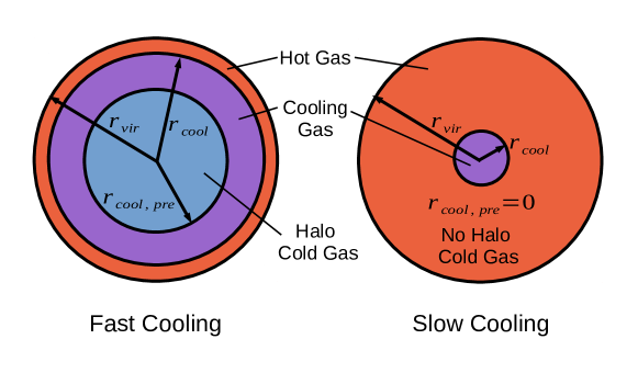
Figure 1: Sketch of the new cooling model.

The above scheme is similar to that in White & Frenk (1991) and to those in many other semi-analytic models, but most of these other models (apart from morgana) do not explicitly introduce the cold gas halo component or the contraction of the hot gas halo. Unlike the morgana model, in which the whole hot gas halo contributes to the cooled down gas in any timestep, here the hot gas cools gradually from halo center outwards. A more detailed discussion of the relation of the new cooling model to those in other semi-analytic models is given in §2.2.

2.1.2 Basic assumptions of the new cooling model

Based on the above picture, we impose our basic assumptions about the cooling as follows:

1. The hot gas in a dark matter halo is in a spherical hot gas halo, with a density distribution described by the so-called $\beta$-distribution:

   $$\rho_{\rm hot}(r)\propto\frac{1}{r^{2}+r_{\rm core}^{2}},\ r_{\rm cool,pre}\leq r\leq r_{\rm vir},$$ (1)

   where $r_{\rm core}$ is called the core radius and is a parameter of this density distribution, while $r_{\rm vir}$ is the virial radius of the dark matter halo, defined as

   $$r_{\rm vir}=\left(\frac{3M_{\rm halo}}{4\pi\Delta_{\rm vir}\overline{\rho}}\right)^{1/3},$$ (2)

   where $\overline{\rho}$ is the mean density of the universe at that redshift, and the overdensity, $\Delta_{\rm vir}(\Omega_{\rm m},\Omega_{\rm v})$, is calculated from the spherical collapse model (e.g. Eke et al., 1996). In galform, typically $r_{\rm core}$ is set to be a fixed fraction of $r_{\rm vir}$ or of the NFW scale radius $r_{\rm NFW}$ (Navarro et al., 1997).

2. The hot gas has only one temperature at any time, and it is set to be the dark matter halo virial temperature $T_{\rm vir}$, where

   $$T_{\rm vir}=\frac{\mu_{\rm m}V_{\rm vir}^{2}}{2k_{\rm B}},$$ (3)

   where $k_{\rm B}$ is the Boltzmann constant, $\mu_{\rm m}$ is the mean mass per particle, and $V_{\rm vir}=(GM_{\rm halo}/r_{\rm vir})^{1/2}$ is the circular velocity at $r_{\rm vir}$.

3. When new gas is added to the hot gas halo, it is assumed to mix homogeneously with the existing hot gas halo. This also means that the hot gas halo has a single metallicity, $Z_{\rm hot}$, at any given time.

4. In the absence of cooling, the specific angular momentum distribution of the hot gas, $j_{\rm hot}(r)\propto r$, corresponding to a mean rotation velocity in spherical shells that is constant with radius. This applies to the initial time when no cooling has happened and also to the gas newly added to the hot gas halo, which is newly heated up. When cooling induces contraction of the hot gas halo, the angular momentum of each Lagrangian hot gas shell is conserved during the contraction, and after this, the rotation velocity is no longer a constant with radius.

Our choices of $\rho_{\rm hot}(r)$ and of the initial $j_{\rm hot}(r)$ follow those of Cole et al. (2000), which are based on hydrodynamical simulations without cooling. This is reasonable because here they only apply to the hot gas.

2.1.3 Cooling calculation

We describe the calculation for a single timestep, starting at time $t$ and ending at time $t+\Delta t$. The timestep, $\Delta t$, should generally be chosen to be small compared to the halo dynamical timescale, so that the evolution in the halo mass and the contraction of the hot gas halo over a timestep are small. At the beginning of each step, $M_{\rm halo}$ is updated according to the halo merger tree, and $r_{\rm vir}$ and $T_{\rm vir}$ are then updated according to the current values of $\Delta_{\rm vir}$ and $\overline{\rho}$. Next, the hot gas density profile, $\rho_{\rm hot}(r,t)$, is updated, which involves two quantities, namely $r_{\rm core}$ and the density normalization. As mentioned above, $r_{\rm core}$ is calculated from the halo radius $r_{\rm vir}$ or $r_{\rm NFW}$. The normalization is fixed by the integral

$$4\pi\int_{r_{\rm cool,pre}(t)}^{r_{\rm vir}(t)}\rho_{\rm hot}(r,t)\,r^{2}dr=M_{\rm hot}(t),$$ (4)

where $M_{\rm hot}$ is the total hot gas mass, and $r_{\rm cool,pre}$ the inner boundary of the hot gas halo at time $t$. Initially $r_{\rm cool,pre}=0$ and is updated (see below) in each timestep for the calculation of the next timestep. For a static halo, $r_{\rm cool,pre}(t)=r_{\rm cool}(t)$, but this no longer applies if the halo grows or the hot gas distribution contracts.

With the density profile determined, the cooling radius $r_{\rm cool}(t+\Delta t)$ at the end of the timestep can be calculated. $r_{\rm cool}$ is defined by

$$t_{\rm cool}(r_{\rm cool},t+\Delta t)=\tilde{t}_{\rm cool,avail}(r_{\rm cool},t+\Delta t),$$ (5)

where $t_{\rm cool}(r,t)$ is the cooling timescale of a shell at radius $r$ at time $t$, and $\tilde{t}_{\rm cool,avail}(r,t)$ is the time available for cooling for that shell. $t_{\rm cool}(r,t)$ is defined as

$$t_{\rm cool}=\frac{\delta U}{\delta L_{\rm cool}}=\frac{3k_{\rm B}}{2\mu_{\rm m}}\frac{T_{\rm vir}}{\tilde{\Lambda}(T_{\rm vir},Z)\rho_{\rm hot}},$$ (6)

where $\delta U$ is the total thermal energy of this shell, while $\delta L_{\rm cool}$ is its current cooling luminosity. For gas with temperature $T_{\rm vir}$ and metallicity $Z_{\rm hot}$, we express the thermal energy density as $(3/2)(\rho_{\rm hot}/\mu_{\rm m})k_{\rm B}T_{\rm vir}$, and the radiative cooling rate per unit volume as $\tilde{\Lambda}(T_{\rm vir},Z_{\rm hot})\rho_{\rm hot}^{2}$, assuming collisional ionization equilibrium. This then leads to the final expression on the RHS above.

The calculation of the time available for cooling, $\tilde{t}_{\rm cool,avail}(r,t)$, is more complicated. For a halo in which the hot gas density distribution, temperature and metallicity are static, and in which the gas started cooling at a halo formation time $t_{\rm form}$, we would define $\tilde{t}_{\rm cool,avail}=t-t_{\rm form}$, as in Cole et al. (2000). However, this definition is not applicable to an evolving halo. Instead, we would like to define a gas shell as having cooled when $\delta U=\delta E_{\rm cool}$, where $\delta U$ is defined as above, and $\delta E_{\rm cool}$ is the total energy that would have been radiated away by this hot gas shell over its past history when we track the shell in a Lagrangian sense. When we calculate $\delta U$ and $\delta E_{\rm cool}$ for a gas shell, we include the effects of evolution in $\rho_{\rm hot}$, $T_{\rm vir}$ and $Z_{\rm hot}$ due to halo growth, reaccretion of ejected gas and contraction of the hot gas. However, in our approach, $\rho_{\rm hot}$ and $T$ in a gas shell are assumed to be unaffected by radiative cooling within that shell, up until the time when the cooling condition is met, when the hot gas shell is assumed to lose all of its thermal energy in a single instant, and be converted to cold gas. Combining the condition $\delta U=\delta E_{\rm cool}$ with equation (6) then leads to a cooling condition of the form $t_{\rm cool}(r,t)=\tilde{t}_{\rm cool,avail}(r,t)$ if $\tilde{t}_{\rm cool,avail}$ for a shell is defined as

$$\tilde{t}_{\rm cool,avail}=\frac{\delta E_{\rm cool}}{\delta L_{\rm cool}}.$$ (7)

This is just the time that it would take for the gas shell to radiate the energy actually radiated over its past history, if it were radiating at its current rate. Note that for a static halo cooling since time $t_{\rm form}$, $L_{\rm cool}$ is constant over the past history of a hot gas shell, so $\delta E_{\rm cool}=\delta L_{\rm cool}\,(t-t_{\rm form})$, and the above definition reduces to $\tilde{t}_{\rm cool,avail}=t-t_{\rm form}$.

The quantity $t_{\rm cool}$ is easy to calculate for each hot gas shell because it only involves quantities at time $t$. In contrast, the calculation of $\tilde{t}_{\rm cool,avail}$ is more difficult, because $\delta E_{\rm cool}$ involves the previous cooling history. To calculate $\tilde{t}_{\rm cool,avail}$ exactly, the cooling history of each Lagrangian hot gas shell would have to be stored. However, this is too computationally expensive for a semi-analytic model, and some further approximations are needed. We first note that for a discrete timestep of length $\Delta t$ and starting at $t$,

$$\tilde{t}_{\rm cool,avail}(r_{\rm cool},t+\Delta t) = \tilde{t}_{\rm cool,avail}(r_{\rm cool},t)+\Delta t$$ (8)

$$\approx \tilde{t}_{\rm cool,avail}(r_{\rm cool,pre},t)+\Delta t.$$ (9)

The first line above comes from the assumption that the hot gas halo is fixed within a given timestep, and thus the increase of $\tilde{t}_{\rm cool,avail}$ over the step is just the increase of the physical time. To justify the approximation in the second line, we consider two cases: (a) $r_{\rm cool}\sim r_{\rm cool,pre}$. In this case, which typically happens when the gas cools slowly compared to the halo dynamical timescale, $\tilde{t}_{\rm cool,avail}(r_{\rm cool},t)\approx\tilde{t}_{\rm cool,avail}(r_{\rm cool,pre},t)$. (b) $r_{\rm cool}\gg r_{\rm cool,pre}$. This typically happens when the gas cools fast compared to the halo dynamical timescale, but in that case, halo growth and hot gas halo contraction play only a weak role in cooling, which means that $\tilde{t}_{\rm cool,avail}$ is nearly the same for all gas shells (as in a completely static halo), so again $\tilde{t}_{\rm cool,avail}(r_{\rm cool},t)\approx\tilde{t}_{\rm cool,avail}(r_{\rm cool,pre},t)$.

Finally, we make the approximation

$$\tilde{t}_{\rm cool,avail}(r_{\rm cool,pre},t)=\frac{\delta E_{\rm cool}(r_{\rm cool,pre},t)}{\delta L_{\rm cool}(r_{\rm cool,pre},t)}\approx\frac{E_{\rm cool}(t)}{L_{\rm cool}(t)}$$ (10)

Here, $L_{\rm cool}$ is the cooling luminosity of the whole hot gas halo at time $t$,

$$L_{\rm cool}(t)=4\pi\int_{r_{\rm cool,pre}}^{r_{\rm vir}}\tilde{\Lambda}(T_{\rm vir},Z_{\rm hot})\,\rho_{\rm hot}^{2}(r,t)\,r^{2}\,dr,$$ (11)

and $E_{\rm cool}(t)$ is the total energy radiated away over its past history by all of the hot gas that is within the halo at time $t$,

$$E_{\rm cool}(t)=4\pi\int_{t_{\rm init}}^{t}\int_{r_{\rm p}(\tau)}^{r_{\rm vir}(\tau)}\tilde{\Lambda}(T_{\rm vir},Z_{\rm hot})\,\rho_{\rm hot}^{2}(r,\tau)\,r^{2}drd\tau.$$ (12)

In the above integral, $t_{\rm init}$ is the starting time for the cooling calculation, and $r_{\rm p}(\tau)$ is the radius at time $\tau$ of the shell that has radius $r_{\rm cool,pre}$ at time $t$.

To justify the approximation made in equation (10), we first note that, due to the integrals in equations (11) and (12) involving $\rho_{\rm hot}^{2}$, both are dominated by the densest regions in the hot gas halo. We now need to consider two cases. (a) $r_{\rm cool,pre}\gtrsim r_{\rm core}$. In this case, the gas density decreases monotonically for $r\gtrsim r_{\rm core,pre}$, so that both integrals are dominated by the contributions from the gas shells near the lower limit of the integral, i.e. near $r_{\rm cool,pre}$. It follows that $E_{\rm cool}(t)/L_{\rm cool}(t)\approx\delta E_{\rm cool}(r_{\rm cool,pre},t)/\delta L_{\rm cool}(r_{\rm cool,pre},t)$. (b) $r_{\rm cool,pre}\lesssim r_{\rm core}$. In this case, $\delta E_{\rm cool}(r,t)/\delta L_{\rm cool}(r,t)$ is approximately independent of radius for $r\lesssim r_{\rm core}$ due to the approximately constant density, while the integrals for $E_{\rm cool}(t)$ and $L_{\rm cool}(t)$ are dominated by the region $r\lesssim r_{\rm core}$, so that we again have $E_{\rm cool}(t)/L_{\rm cool}(t)\approx\delta E_{\rm cool}(r_{\rm cool,pre},t)/\delta L_{\rm cool}(r_{\rm cool,pre},t)$.

By combining equations (9) and (10), we obtain the expression for $t_{\rm cool,avail}$ that we actually use:

$$t_{\rm cool,avail}(t+\Delta t) = \frac{E_{\rm cool}(t)}{L_{\rm cool}(t)}+\Delta t$$ (13)

$$\approx \tilde{t}_{\rm cool,avail}(r_{\rm cool},t+\Delta t),$$

In the above, the term $E_{\rm cool}(t)/L_{\rm cool}(t)$ represents the available time at the start of the step, calculated from the previous cooling history.

The calculation of $E_{\rm cool}$ from equation (12) appears to require storing the histories of all of the shells of hot gas in order to evaluate the integral. However, from its definition, it is easy to derive an approximate recursive equation for it (see Appendix A)

$$E_{\rm cool}(t+\Delta t) \approx E_{\rm cool}(t)+L_{\rm cool}(t)\times\Delta t$$ (14)

$$- L^{\prime}_{\rm cool}(t)\times t_{\rm cool,avail}(t+\Delta t),$$

where

$$L^{\prime}_{\rm cool}(t)=4\pi\int_{r_{\rm cool,pre}}^{r_{\rm cool}}\tilde{\Lambda}(T_{\rm vir},Z_{\rm hot})\,\rho_{\rm hot}^{2}\,r^{2}\,dr.$$ (15)

The second term in equation (14) adds the energy radiated away in the current timestep, while the third term removes the contribution from gas between $r_{\rm cool,pre}$ and $r_{\rm cool}$, because it cools down in the current timestep and therefore is not part of the hot gas halo at the next timestep. Starting from the initial value $E_{\rm cool}=0$, equation (14) can be used to derive $E_{\rm cool}$ for the subsequent timesteps, and then equations (5), (6) and (13) can be used to calculate $r_{\rm cool}$. For a static halo, in which there is no accretion and no contraction of the hot gas, it can be shown that equations (13)-(15) lead to $t_{\rm avail}(t+\Delta t)=t+\Delta t-t_{\rm init}$, the same as in Cole et al. (2000).

With $r_{\rm cool,pre}$ and $r_{\rm cool}$ determined, the mass and angular momentum of the gas cooled down over the time interval $(t,t+\Delta t)$ are calculated from

$$\Delta M_{\rm cool} = 4\pi\int_{r_{\rm cool,pre}}^{r_{\rm cool}}\rho_{\rm hot}r^{2}dr$$ (16)

$$\Delta J_{\rm cool} = 4\pi\int_{r_{\rm cool,pre}}^{r_{\rm cool}}j_{\rm hot}\rho_{\rm hot}r^{2}dr,$$ (17)

where $j_{\rm hot}(r)$ is the specific angular momentum distribution of the hot gas, which is calculated as described in §2.1.4. $\Delta M_{\rm cool}$ and $\Delta J_{\rm cool}$ are used to update the mass, $M_{\rm halo,cold}$, and angular momentum, $J_{\rm halo,cold}$, of the cold halo gas component.

Gas in the cold halo gas component is not pressure supported, and so is assumed to fall to the central galaxy in the halo on the freefall timescale. We therefore calculate the mass, $\Delta M_{\rm acc,gal}$, and angular momentum, $\Delta J_{\rm acc,gal}$, accreted onto the central galaxy over a timestep as

$$\Delta M_{\rm acc,gal} = M_{\rm halo,cold}\times\min[1,\Delta t/t_{\rm ff}(r_{\rm cool})]$$ (18)

$$\Delta J_{\rm acc,gal} = J_{\rm halo,cold}\times\min[1,\Delta t/t_{\rm ff}(r_{\rm cool})]$$ (19)

where $t_{\rm ff}(r_{\rm cool})$ is the free-fall time scale at the cooling radius. Note that in the slow cooling regime, where $t_{\rm ff}(r_{\rm cool})<t_{\rm cool}(r_{\rm cool})$, the mass of the cold halo gas component remains relatively small, since the timescale for draining it ($t_{\rm ff}$) is short compared to the timescale for feeding it ($t_{\rm cool}$).

Note that here we treat the angular momentum of the cooled down gas as a scalar. This means that the axis of the galaxy spin is assumed to be always aligned with the axis of the hot gas halo spin. We adopt this assumption mainly because the halo spin parameter, which is the basis of the calculation of hot gas angular momenta, only contains information on the magnitude of the angular momentum. This is an important limitation, and a calculation of the angular momentum of the hot gas considering both its magnitude and direction should be developed. However, this is beyond the scope of this paper, and we leave it for future work.

Finally, we consider the contraction of the hot gas halo. The gas between the cooling radius and the virial radius is assumed to remain in approximate hydrostatic equilibrium, so for simplicity we assume that it always follows the $\beta$-profile. The hot gas at the cooling radius is not pressure-supported by the cold gas at smaller radii, so we assume that this gas contracts towards the halo centre on a timescale $t_{\rm ff}(r_{\rm cool})$. The new $r_{\rm cool,pre}$ at the next timestep starting at $t+\Delta t$ is therefore estimated as

$$r_{\rm cool,pre}(t+\Delta t)=r_{\rm cool}(t+\Delta t)\times\max[0,1-\Delta t/t_{\rm ff}(r_{\rm cool})].$$ (20)

The above equation only applies if the gravitational potential of the halo is fixed. When the halo grows in mass, and when the mean halo density within $r_{\rm vir}$ adjusts with the mean density of the universe, the gravitational potential also changes, and this affects the contraction of the hot gas halo. We estimate the effect of this on the inner boundary of the hot halo gas by requiring that the mass of dark matter contained inside $r_{\rm cool,pre}$ remains the same before and after the change in the halo potential, i.e.

$$M^{\prime}_{\rm halo}[r^{\prime}_{\rm cool,pre}(t+\Delta t)]=M_{\rm halo}[r_{\rm cool,pre}(t+\Delta t)],$$ (21)

where the quantities with apostrophes are after halo growth, while those without apostrophes are before halo growth. The reason for using the dark matter to trace this contraction is that the gas within $r_{\rm cool,pre}$ is cold with negligible pressure effects, so its dynamics should be similar to those of the collisionless dark matter.

2.1.4 Calculating $j_{\rm hot}(r)$

The specific angular momentum of the hot gas averaged over spherical shells is assumed to follow $j_{\rm hot}(r)\propto r$ at the initial time, as stated in §2.1.2, with the normalization set by the assumption that the mean specific angular momentum of the hot gas in the whole halo, $\overline{j}_{\rm hot}$, is initially equal to that of the dark matter, $J_{\rm halo}/M_{\rm halo}$ (see §2.3). Later on, the dark matter halo growth, the contraction of the hot gas halo and the addition of new gas all can change the angular momentum profile. In this new cooling model, at the beginning of each timestep, we first consider the angular momentum profile change of the existing hot gas due to the hot gas halo contraction and the dark matter halo growth that took place during the last timestep, and then add the contribution from the newly added hot gas to this adjusted profile.

In deriving the change of angular momentum profile of the existing hot gas, we assume mass and angular momentum conservation for each Lagrangian shell. Consider a shell with mass $dm$, original radius $r$ and specific angular momentum $j_{\rm hot}(r)$, which, after the dark matter growth and hot gas halo contraction, moves to radius $r^{\prime}$ with specific angular momentum $j^{\prime}_{\rm hot}(r^{\prime})$. The shell mass is unchanged because of mass conservation. Then angular momentum conservation implies $j^{\prime}_{\rm hot}(r^{\prime})=j_{\rm hot}(r)$. In other words, the angular momentum profile after these changes is $j_{\rm hot}[r(r^{\prime})]$. Given $j_{\rm hot}(r)$ from the last timestep, the major task for deriving $j^{\prime}_{\rm hot}(r^{\prime})$ is to derive $r(r^{\prime})$. This can be done by considering shell mass conservation and the density profiles of the hot gas. Specifically, assuming $\rho_{\rm hot}(r)$ and $\rho^{\prime}_{\rm hot}(r^{\prime})$ are respectively the density profiles of the existing hot gas before and after the dark matter halo growth and hot gas halo contraction, then one has

$$4\pi\rho_{\rm hot}(r)r^{2}dr=dm=4\pi\rho^{\prime}_{\rm hot}(r^{\prime})r^{\prime 2}dr^{\prime}.$$ (22)

This, together with the assumption that $\rho_{\rm hot}(r)$ and $\rho^{\prime}_{\rm hot}(r^{\prime})$ follow the $\beta$-distribution, can then be solved for $r(r^{\prime})$. Unfortunately, this equation can only provide an implicit form for $r^{\prime}(r)$, and does not lead to an explicit analytical expression for $j^{\prime}_{\rm hot}(r^{\prime})$. A straightforward way to deal with this is to evaluate $j^{\prime}_{\rm hot}(r^{\prime})$ numerically for a grid of radii and then store this information, however, this is computationally expensive. Instead, we apply further approximations to reduce the computational cost of solving for $j^{\prime}_{\rm hot}(r^{\prime})$, as described in detail in Appendix B.

To derive the final angular momentum distribution, $j^{\prime\prime}_{\rm hot}(r^{\prime})$, one still needs to consider the contribution from the newly added hot gas. Assuming the gas newly added to a given shell with radius $r^{\prime}$ has mass $dm_{\rm new}$ and specific angular momentum $j_{\rm new}(r^{\prime})$, then one has

$$j^{\prime\prime}_{\rm hot}(r^{\prime})(dm+dm_{\rm new})=j^{\prime}_{\rm hot}(r^{\prime})dm+j_{\rm new}(r^{\prime})dm_{\rm new}.$$ (23)

Since the newly added gas is assumed to be mixed homogeneously with the hot gas halo, so all $dm_{\rm new}/(dm+dm_{\rm new})$ should be the same for all shells, and hence

$$\frac{dm_{\rm new}}{dm_{\rm new}+dm}=\frac{M_{\rm new}}{M_{\rm new}+M_{\rm old}},$$ (24)

where $M_{\rm new}$ is the total mass added to the hot gas halo during the timestep, while $M_{\rm old}$ is the previous mass.

Further, according to the assumption in §2.1.2, $j_{\rm new}(r^{\prime})\propto r^{\prime}$. In general, there are two components to the newly added hot gas: (a) gas brought in through growth of the dark matter halo; and (b) gas that has been ejected from the galaxy by SN feedback, has joined the ejected gas reservoir, and then has been reaccreted into the hot gas halo. Their contributions to the total angular momentum of the newly added gas are described in §2.1.5. With this, the normalization of $j_{\rm new}(r^{\prime})$ can be determined.

Finally, with $j^{\prime}_{\rm hot}(r^{\prime})$ and $j_{\rm new}(r^{\prime})$ known, the specific angular momentum distribution at the current timestep, $j^{\prime\prime}_{\rm hot}(r^{\prime})$, is determined as

$$j^{\prime\prime}_{\rm hot}(r^{\prime})(M_{\rm new}+M_{\rm old})=j^{\prime}_{\rm hot}(r^{\prime})M_{\rm old}+j_{\rm new}(r^{\prime})M_{\rm new}.$$ (25)

In this way, the specific angular momentum distribution for any given timestep can be derived recursively from the initial distribution.

2.1.5 Treatments of gas ejected by feedback and halo mergers

The SN feedback can heat and eject gas in galaxies, and the ejected gas is added to the so-called ejected gas reservoir. This transfers mass and angular momentum from galaxies to that reservoir. The gas ejected from both the central galaxy and its satellites is added to the ejected gas reservoir of the central galaxy. The ejected mass is determined by the SN feedback prescription, and is typically proportional to the instantaneous star formation rate. The angular momentum of this ejected gas is calculated as follows.

The total angular momentum of the ejected gas can be expressed as the product of its mass and its specific angular momentum. For the gas ejected from the central galaxy, its specific angular momentum is estimated as that of the central galaxy, while for the gas ejected from satellites, its specific angular momentum is estimated as the mean specific angular momentum of the central galaxy’s host dark matter halo, i.e. $J_{\rm halo}/M_{\rm halo}$, in order roughly to include the contribution to the ejected angular momentum from the satellite orbital motion. This is only a rough estimate. A better estimate would be obtained by following the satellite orbit, but we leave this for future work.

This ejected gas can later be reaccreted onto the hot gas halo, thus delivering mass and angular momentum to it. The reaccretion rates of mass and angular momentum are respectively estimated as

$$\dot{M}_{\rm return} = \alpha_{\rm return}\times M_{\rm eject}/t_{\rm dyn}$$ (26)

$$\dot{J}_{\rm return} = \alpha_{\rm return}\times J_{\rm eject}/t_{\rm dyn},$$ (27)

where $\dot{M}_{\rm return}$ and $\dot{J}_{\rm return}$ are respectively the mass and angular momentum reaccretion rates, $M_{\rm eject}$ and $J_{\rm eject}$ are respectively the total mass and angular momentum of the ejected gas reservoir, $t_{\rm dyn}=r_{\rm vir}/v_{\rm vir}$ is the halo dynamical timescale and $\alpha_{\rm return}\sim 1$ a free parameter. For a timestep of finite length $\Delta t$, the mass and angular momentum reaccreted within it is then calculated as the products of the corresponding rates and $\Delta t$.

When a halo falls into a larger halo, it becomes a subhalo, while the larger one becomes the host halo of this subhalo. The halo gas in the subhalo could be ram-pressure or tidally stripped. This process can be calculated within the semi-analytic framework [see e.g. Font et al. (2008) or Guo et al. (2011)], but here we assume for simplicity that the relevant gas is instantaneously removed on infall. The new cooling model assumes that the hot gas and ejected gas reservoir associated with this subhalo are instantaneously transferred to the corresponding gas components of the host halo at infall. The masses of these transferred components can be simply added to the corresponding components of the host halo. However, the angular momentum cannot be directly added, because it is calculated before infall, when the subhalo was still an isolated halo, and the reference point for this angular momentum is the centre of the subhalo, while after the transition, the reference point becomes the centre of the host halo.

Here the angular momentum transferred is estimated as follows. The total angular momentum transferred is expressed as a product of the total transferred mass and the specific angular momentum. The latter one is estimated as $j_{\rm new,halo}=\Delta J_{\rm halo}/\Delta M_{\rm halo}$, where $\Delta J_{\rm halo}$ and $\Delta M_{\rm halo}$ are the angular momentum and mass changes in dark matter halo during the halo merger, and they can be determined when the mass and spin, $\lambda_{\rm halo}$, of each halo in a merger tree are given (see §2.3). The reason for this estimation is that the dark matter and baryon matter accreted by the host halo have roughly the same motion, and thus should gain similar specific angular momentum through the torque exerted by the surrounding large-scale structures. The mass and angular momentum transferred during the halo merger can be summarized as:

$$\Delta M_{\rm hot,mrg} = \sum_{i=1}^{N_{\rm mrg}}M_{\rm hot,i},$$ (28)

$$\Delta J_{\rm hot,mrg} = j_{\rm new,halo}\times\Delta M_{\rm hot,mrg},$$ (29)

$$\Delta M_{\rm eject,mrg} = \sum_{i=1}^{N_{\rm mrg}}M_{\rm eject,i},$$ (30)

$$\Delta J_{\rm eject,mrg} = j_{\rm new,halo}\times\Delta M_{\rm eject,mrg},$$ (31)

where $\Delta M_{\rm hot,mrg}$ and $\Delta J_{\rm hot,mrg}$ are respectively the total mass and angular momentum transferred to the hot gas halo of the host halo during the halo merger, while $\Delta M_{\rm eject,mrg}$ and $\Delta J_{\rm eject,mrg}$ are the mass and angular momentum transferred to the ejected gas reservoir; $N_{\rm mrg}$ is the total number of infalling haloes over the timestep, $M_{\rm hot,i}$ is the total mass of the hot gas halo of the $i$th infalling halo, and $M_{\rm eject,i}$ is the mass of its ejected gas reservoir.

In this cooling model, by default, the halo cold gas is not transferred during halo mergers, because it is cold and in the central region of the infalling halo, and thus is less affected by ram pressure and tidal stripping. After infall, this cold gas halo can still deliver cold gas to the satellite for a while. There are also options in the code to transfer the halo cold gas to the hot gas halo or halo cold gas of the host halo. In this work, we always adopt the default setting.

A dark matter halo may also accrete smoothly. The accreted gas is assumed to be shock heated and join the hot gas halo. In each timestep, the mass of this gas, $\Delta M_{\rm hot,smooth}$, is given as $\Delta M_{\rm hot,smooth}=[\Omega_{\rm b}/\Omega_{\rm m}]\Delta M_{\rm halo,smooth}$, with $\Delta M_{\rm halo,smooth}$ the mass of smoothly accreted dark matter, which is provided by the merger tree, while the associated angular momentum is estimated as $\Delta J_{\rm hot,smooth}=j_{\rm new,halo}\times\Delta M_{\rm hot,smooth}$.

In each timestep, $\Delta M_{\rm return}$, $\Delta M_{\rm hot,mrg}$ and $\Delta M_{\rm hot,smooth}$ increase the mass of the hot gas halo, but do not increase $E_{\rm cool}$. This means the newly added gas has no previous cooling history, consistently with the assumption that this gas is newly heated up by shocks. The total angular momentum of this newly added gas is $\Delta J_{\rm return}+\Delta J_{\rm hot,mrg}+\Delta J_{\rm hot,smooth}$, and, together with the assumption that $j_{\rm new}(r)\propto r$, it completely determines the specific angular momentum distribution of the newly added gas.

2.2 Previous cooling models

2.2.1 galform cooling model GFC1

The GFC1 (GalForm Cooling 1) cooling model is used in all recent versions of galform (e.g. Gonzalez-Perez et al., 2014; Lacey et al., 2016), and is based on the cooling model introduced in Cole et al. (2000), and modified in Bower et al. (2006). The Cole et al. (2000) cooling model introduced so-called halo formation events. These are defined such that the appearance of a halo with no progenitor in a merger tree is a halo formation event, and the time when a halo first becomes at least twice as massive as at the last halo formation event is a new halo formation event. The Cole et al. model then assumes that the hot gas halo is set between two adjacent halo formation events, and is reset at each formation event. Under this assumption, $\tilde{t}_{\rm cool,avail}(r_{\rm cool},t)$ is always the time elapsed since the latest halo formation event, which is straightforward to calculate. As in the new cooling model, we denote the actual $\tilde{t}_{\rm cool,avail}(r_{\rm cool},t)$ used in this model as $t_{\rm cool,avail}(t)$. With $t_{\rm cool,avail}$ given, $r_{\rm cool}$ can be then calculated from equation (5), and the mass and angular momentum cooled down can be calculated as described below. The assumption of a fixed hot gas halo between two halo formation events means that changes in $r_{\rm vir}$ and $T_{\rm vir}$ induced by halo growth, and by the addition of new hot gas either by halo growth or by the reincorporation of gas ejected by feedback between halo formation events, are not considered until the coming of a halo formation event. While this may be reasonable for halo formation events induced by halo major mergers, in which the hot gas halo properties change fairly abruptly, it is not physical if the halo formation event is triggered through smooth halo growth, in which case the changes in the hot gas halo should also happen smoothly, instead of happening in a sudden jump at the halo formation event.

The GFC1 model (Bower et al., 2006) improves the Cole et al. model by updating some hot gas halo properties at each timestep instead of only at halo formation events. Specifically, the hot gas is still assumed to settle in a density profile described by the $\beta$-distribution, with temperature equal to the current halo virial temperature, $T_{\rm vir}$, and $r_{\rm core}$ set to be a fixed fraction of the current $r_{\rm vir}$. The halo mass is updated at each timestep, and the total hot gas mass and metallicity include the contributions from the hot gas newly added at each timestep. However, $V_{\rm vir}$ and $T_{\rm vir}$ are fixed at the values calculated at the last halo formation event. Unlike in the new cooling model, the normalization of the density profile is determined by requiring that

$$4\pi\int_{0}^{r_{\rm vir}}\rho_{\rm hot}r^{2}dr=M_{\rm hot}+M_{\rm cooled},$$ (32)

where $M_{\rm hot}$ is the total mass of the hot gas, while $M_{\rm cooled}$ is the total mass of the gas that has cooled down from this halo since the last halo formation event, and is either in the central galaxy or ejected by SN feedback but not yet reaccreted by the hot gas halo. Accordingly, $M_{\rm cooled}$ is reset to $0$ at each halo formation event, while the ejected gas reservoir mass, $M_{\rm eject}$, evolves smoothly and is not affected by halo formation events.

This is not very physical because the cooled down gas might have collapsed onto the central galaxy long ago, while the ejected gas is outside the halo. This also means that the contraction of the hot gas halo due to cooling is largely ignored in the determination of its density profile. This point is most obvious in the case of a static halo, when the dark matter halo does not grow. In this case, if there is no feedback and subsequent reaccretion, then the amount of hot gas gradually reduces due to cooling, and the hot gas halo should gradually contract in response to the reduction of pressure support caused by this cooling. However, in the GFC1 model, in this situation, the hot gas profile remains fixed, because $M_{\rm hot}+M_{\rm cooled}$ always equals the initial total hot gas mass. For a dynamical halo, $M_{\rm cooled}$ is reset to zero at each halo formation event, and thus the hot gas contracts to halo center at these events. In this way, the halo contraction due to cooling is included to some extent.

In the GFC1 model $r_{\rm cool}$ is calculated in the same way as in Cole et al. (2000). For the estimation of $\tilde{t}_{\rm cool,avail}(r_{\rm cool},t)$, the GFC1 model retains the artificial halo formation events. This means that in both the GFC1 and Cole et al. (2000) cooling models, the hot gas cooling history is effectively reset at each halo formation event. While this might be physical when the halo grows through major mergers, it is artificial when a halo grows smoothly, in which case the cooling history is expected to evolve smoothly as well. Moreover, in principle $\tilde{t}_{\rm cool,avail}(r_{\rm cool},t)$ should change when the hot gas halo changes, which happens between halo formation events in the GFC1 model, so estimating $\tilde{t}_{\rm cool,avail}(r_{\rm cool},t)$ in the GFC1 model in the same way as in Cole et al. (2000) is not self-consistent.

Unlike the new cooling model that explicitly introduces a cold halo gas component that drains onto the central galaxy on the free-fall timescale, the GFC1 and Cole et al. (2000) cooling models introduce a free-fall radius, $r_{\rm ff}$, to allow for the fact that gas cannot accrete onto the central galaxy more rapidly than on a free-fall timescale, no matter how rapidly it cools. $r_{\rm ff}$ is calculated as

$$t_{\rm ff}(r_{\rm ff})=t_{\rm ff,avail},$$ (33)

where $t_{\rm ff}(r)$ is the free-fall timescale at radius $r$, defined as the time for a particle to fall to $r=0$ starting at rest at radius $r$, and $t_{\rm ff,avail}$ is the time available for free-fall, which is set to be the same as $t_{\rm cool,avail}$ in these two cooling models. Then, the mass accreted onto the cental galaxy over a timestep is given by

$$\Delta M_{\rm acc,gal}=4\pi\int_{r_{\rm infall,pre}}^{r_{\rm infall}}\rho_{\rm hot}\,r^{2}dr,$$ (34)

where $\rho_{\rm hot}$ is the current halo gas density distribution, while $r_{\rm infall}=\min(r_{\rm cool},r_{\rm ff})$, and $r_{\rm infall,pre}$ is determined by $4\pi\int_{0}^{r_{\rm infall,pre}}\rho_{\rm hot}r^{2}dr=M_{\rm cooled}$.

The introduction of $r_{\rm ff}$ and $r_{\rm infall}$ leaves part of the cooled down gas in the nominal hot gas halo when $r_{\rm cool}>r_{\rm ff}$, which is the case in the fast cooling regime. This gas is treated as hot gas in subsequent timesteps. While in the fast cooling regime this should not strongly affect the final results for the amount of gas that cools, due to the cooling and accretion being rapid, this misclassification of cold gas as hot is still an unwanted physical feature of a cooling model.

The calculation of the angular momentum of the gas accreted onto the central galaxy is the same in the cooling model in Cole et al. (2000) and GFC1 model. The angular momentum is calculated as

$$\Delta J_{\rm acc,gal}=4\pi\int_{r_{\rm infall,pre}}^{r_{\rm infall}}j_{\rm hot}\rho_{\rm hot}r^{2}dr,$$ (35)

where $j_{\rm hot}$ is the specific angular momentum distribution of the hot gas halo, which is assumed to vary as $j_{\rm hot}\propto r$. As mentioned in §2.1.2, this assumption is based on hydrodynamical simulations without cooling. Assuming it applies unchanged in the presence of cooling means that the effect of contraction of the hot gas halo due to cooling is ignored.

This model adopts treatments for the gas ejected by feedback and for halo mergers similar to those of the new cooling model. Since the GFC1 model assumes that $t_{\rm cool,avail}$ is always the physical time since the last halo formation event, here the gas newly added through halo growth and reaccretion of the feedback ejected gas would share this $t_{\rm cool,avail}$ and thus implicitly gain some previous cooling history. As a result, the newly added gas is effectively not actually newly heated up.

2.2.2 galform cooling model GFC2

The GFC2 (GalForm Cooling 2) model was introduced by Benson & Bower (2010). It makes several improvements over the GFC1 model. The assumptions about the density profile, temperature and metallicity of the hot gas halo are the same as in GFC1, but the influence of halo formation events is mostly removed. The density profile of the hot gas is normalized by requiring

$$4\pi\int_{0}^{r_{\rm vir}}\rho_{\rm hot}r^{2}dr=M_{\rm hot}+M_{\rm cooled}+M_{\rm eject},$$ (36)

where $M_{\rm eject}$ is the mass of gas ejected by SN feedback and not yet reaccreted, while the definition of $M_{\rm cooled}$ is modified: (a) It is incremented by the mass cooled and accreted onto the central galaxy, and reduced by the mass ejected by SN feedback. (b) A gradual reduction of $M_{\rm cooled}$ as

$$\dot{M}_{\rm cooled}=-\alpha_{\rm remove}\times M_{\rm cooled}/t_{\rm ff}(r_{\rm vir}),$$ (37)

with $\alpha_{\rm remove}\sim 1$ being a free parameter. (c) When a halo merger occurs, the value of $M_{\rm cooled}$ is propagated to the current halo from its most massive progenitor (rather than being reset to 0 at each halo formation event as in the GFC1 model). Since the density profile normalization for the hot gas is determined by equation (36), for a given $M_{\rm hot}$ and $M_{\rm eject}$, the gradual reduction of $M_{\rm cooled}$ due to equation (37) lowers the normalization, and so to include the same mass, $M_{\rm hot}$, in the density profile, the hot gas must be distributed to smaller radii. This gradual reduction of $M_{\rm cooled}$ thus effectively leads to a contraction of the hot gas halo in response to the removal of hot gas by cooling, which is more physical than the treatment in the GFC1 model. However, here the timescale for this contraction is $t_{\rm ff}(r_{\rm vir})$, while the region where the contraction happens has a radius $\sim r_{\rm cool}$, so there is still a physical mismatch in this scale. This is improved in the new cooling model introduced in §2.1, where the timescale $t_{\rm ff}(r_{\rm cool})$ is adopted instead.

In the GFC2 model, as in the new cooling model, $r_{\rm cool}$ is calculated using equation (5), with $\tilde{t}_{\rm cool,avail}(r_{\rm cool},t)$ being estimated from the energy radiated away. By doing this, the effect of artificial halo formation events on the gas cooling is largely removed. However, instead of directly accumulating this radiated energy as in the new cooling model, the GFC2 model further approximates the integrals involving $\rho_{\rm hot}^{2}$ in equations (11) and (12) as

$$4\pi\int_{0}^{r_{\rm vir}}\rho^{2}_{\rm hot}r^{2}dr \approx \bar{\rho}_{\rm hot}\times 4\pi\int_{0}^{r_{\rm vir}}\rho_{\rm hot}r^{2}dr$$ (38)

$$= \bar{\rho}_{\rm hot}(M_{\rm hot}+M_{\rm cooled}+M_{\rm eject}),$$

where $\bar{\rho}_{\rm hot}$ is the mean density given by the density profile. This approximation is very rough, and while in the new cooling model the integral is limited to the gas that is hot, i.e. between $r_{\rm cool,pre}$ and $r_{\rm vir}$, in the GFC2 model the integration range is extended to $r=0$, which, according to equation (36), includes the part of the density profile where the gas has already cooled down. These approximations make the calculation of $\tilde{t}_{\rm cool,avail}(r_{\rm cool},t)$ faster but less accurate and physical than in the new cooling model.

With these approximations, for any time $t$, the GFC2 model adopts the following equations in place of equations (11) and (12) in the new cooling model:

$$L_{\rm cool}(t) = \tilde{\Lambda}(T_{\rm vir},Z)\bar{\rho}_{\rm hot}(M_{\rm hot}+M_{\rm cooled}+M_{\rm eject})$$ (39)

$$E_{\rm cool}(t) = \int_{t_{\rm init}}^{t}\tilde{\Lambda}(T_{\rm vir},Z)\bar{\rho}_{\rm hot}\times$$ (40)

$$[M_{\rm hot}(\tau)+M_{\rm cooled}(\tau)+M_{\rm eject}(\tau)]d\tau$$

$$+ \int_{t_{\rm init}}^{t}\frac{3k_{\rm B}}{2\mu_{\rm m}}T_{\rm vir}\dot{M}_{\rm cooled}d\tau.$$

The second term in equation (40), which is negative, is equal in absolute value to the total thermal energy of the cooled mass removed according to equation (37), and is designed to remove the contribution to $E_{\rm cool}$ from this cooled mass. Given $E_{\rm cool}$ and $L_{\rm cool}$, $\tilde{t}_{\rm cool,avail}(r_{\rm cool},t)$ for a given timestep is calculated from equation (13), as in the new model. Again, the actual $\tilde{t}_{\rm cool,avail}(r_{\rm cool},t)$ used in this model is denoted as $t_{\rm cool,avail}(t)$. Note that the approximation made in equation (38) leads to the derived $t_{\rm cool,avail}$ being closer to the average cooling history of all shells instead of the cooling history of gas near $r_{\rm cool}$, and so leads to less accurate results than in the new cooling model.

The GFC2 model allows for the effect of the free-fall timescale on the gas mass accreted onto the central galaxy in a similar way to the GFC1 model, by introducing the radius, $r_{\rm ff}$, calculated from equation (33), but with $t_{\rm ff,avail}$ calculated in a way similar to that for $t_{\rm cool,avail}$. Specifically, a quantity with dimensions of energy similar to $E_{\rm cool}$ is accumulated for $t_{\rm ff,avail}$, but this quantity has an upper limit, $t_{\rm ff}(r_{\rm vir})\times L_{\rm cool}$, and once it exceeds this limit, it is then reset to this limit value. This limit ensures $t_{\rm ff,avail}\leq t_{\rm ff}(r_{\rm vir})$. Note that the effect of imposing this limit is usually to lead to a $t_{\rm ff,avail}$ different from both $t_{\rm cool,avail}$ and $t_{\rm ff}(r_{\rm vir})$. This calculation of $t_{\rm ff,avail}$ is not very physical because the calculation of $t_{\rm cool,avail}$ here is based approximately on the total energy released by the cooling radiation, while the accretion of the cooled gas onto the central galaxy is driven by gravity, which does not depend on the energy lost by radiation. In addition, by introducing $r_{\rm ff}$, the GFC2 model inherits the associated problems already identified for the GFC1 model.

The GFC2 model also adopts a specific angular momentum distribution for the hot gas to calculate the angular momentum of the gas that cools down and accretes onto the central galaxy. The simpler method to specify this angular momentum distribution is as a function of radius, namely $j_{\rm hot}(r)$. But, in principle, this requires calculating the subsequent evolution of $j_{\rm hot}(r)$ as the hot gas halo contracts, which is considered in the new cooling model but not in the GFC1 or GFC2 models. A more complex method is to specify $j_{\rm hot}$ as a function of the gas mass enclosed by a given radius, i.e. $j_{\rm hot}(<M)$. This implicitly includes the effect of contraction of the hot gas halo in the case of a static halo, where no new gas joins the hot gas halo, because while the radius of each gas shell changes during contraction , the enclosed mass is kept constant and can be used to track each Lagrangian shell. However, when there is new gas being added to the hot gas halo, this method also fails, because the newly joining gas mixes with the hot gas halo after contraction, and, in this case, the contraction has to be considered explicitly. Since even the more complex method is not fully self-consistent, for the sake of simplicity, in this work we adopt the simpler method to calculate the angular momentum, without allowing for contraction of the hot gas halo.

This model also adopts the treatments for the gas ejected by feedback and for halo mergers similar to those of the new cooling model, but unlike in the latter, here $E_{\rm cool}$ of the hot gas in the infalling haloes is also transferred. This again gives the newly added gas some previous cooling history, so it is not newly heated up.

2.2.3 Cooling model in l-galaxies

The cooling model used in l-galaxies (see e.g. Croton et al. 2006; Guo et al. 2011; Henriques et al. 2015) assumes that the hot gas is always distributed from $r=0$ to $r=r_{\rm vir}$, and that its density profile is singular isothermal, namely $\rho_{\rm hot}(r)\propto r^{-2}$, with a single metallicity and a single temperature equaling $T_{\rm vir}$. The total mass inside this profile is $M_{\rm hot}$.

Then, a cooling radius, $r_{\rm cool}$, is calculated from $t_{\rm cool}(r_{\rm cool})=t_{\rm cool,avail}$, with $t_{\rm cool,avail}=t_{\rm dyn}=r_{\rm vir}/V_{\rm vir}$. If $r_{\rm cool}\leq r_{\rm vir}$, then the mass accreted onto the central galaxy in a timestep, $\Delta t$, is

$$\Delta M_{\rm acc,gal} = 4\pi\rho_{\rm hot}(r_{\rm cool})\times r_{\rm cool}^{2}\frac{dr_{\rm cool}}{dt}\Delta t$$ (41)

$$= \frac{M_{\rm hot}}{r_{\rm vir}}\frac{r_{\rm cool}}{t_{\rm dyn}}\Delta t,$$

with $dr_{\rm cool}/dt$ being estimated as $dr_{\rm cool}/dt=r_{\rm cool}/t_{\rm cool,avail}=r_{\rm cool}/t_{\rm dyn}$. If instead $r_{\rm cool}>r_{\rm vir}$, then

$$\Delta M_{\rm acc,gal}=\frac{M_{\rm hot}}{t_{\rm dyn}}\Delta t.$$ (42)

Note that earlier predecessors of the l-galaxies model made slightly different assumptions. Kauffmann et al. (1993) and subsequent papers in that series followed the approach of White & Frenk (1991), assuming that $t_{\rm cool,avail}=t$, with $t$ being the age of the Universe, and also that $dr_{\rm cool}/dt=r_{\rm cool}/(2t_{\rm cool,avail})$, where the latter follows mathematically from the result that $r_{\rm cool}\propto t^{1/2}$ for a static halo with $\rho_{\rm hot}(r)\propto r^{-2}$ and $T_{\rm hot}(r)={\rm const}$. Springel et al. (2001) modified the first of these assumptions by instead assuming $t_{\rm cool,avail}=t_{\rm dyn}$. This change in $t_{\rm cool,avail}$ was effectively justified by the work of Yoshida et al. (2002), who compared the l-galaxies cooling model with results from the “stripped-down” cosmological gasdynamical simulation of galaxy formation described below. As described in Guo et al. (2011), versions of l-galaxies from Croton et al. (2006) onwards then changed to using $dr_{\rm cool}/dt=r_{\rm cool}/t_{\rm cool,avail}$. This originates from an erroneous omission of the factor $0.5$ in the l-galaxies code (see the footnote to equation (5) in Guo et al. for more details). Note that the SAGE model (e.g. Croton et al., 2016) uses the same cooling model, but keeps the factor $1/2$, adopting $dr_{\rm cool}/dt=r_{\rm cool}/(2t_{\rm dyn})$.

The l-galaxies cooling model is motivated by the self-similar cooling solution for a static halo derived in Bertschinger (1989), in which the evolution of the hot gas profile driven by cooling is expressed in terms of a characteristic scale length $r_{\rm cool}(t)$. Bertschinger defines $r_{\rm cool}$ by $t_{\rm cool}(r_{\rm cool})=t$, where $t_{\rm cool}(r)$ is the cooling timescale profile of the hot gas profile at the initial time, i.e. before the start of cooling, while $t$ is the physical time elapsed since then. Bertschinger found that the mass accretion rate onto the centre is approximately the same as the mass cooling rate at $r_{\rm cool}$, leading to an expression similar to the first line of equation (41). Note that the $r_{\rm cool}$ introduced in Bertschinger (1989) is a scale radius in the hot gas profile, while the $r_{\rm cool}$ in other cooling models considered in this paper is the inner boundary of the hot gas halo, which separates hot and cooled down gas, and thus they have different physical meanings.

However, the Bertschinger (1989) solution does not provide a complete justification for the l-galaxies cooling model. The l-galaxies cooling model does not follow the original definition of $r_{\rm cool}$ in Bertschinger (1989). It instead defines $r_{\rm cool}$ as $t_{\rm cool}(r_{\rm cool})=t_{\rm dyn}$, where $t_{\rm cool}(r)$ is the cooling timescale profile of the current hot gas halo (including the evolution of the density of the hot gas halo driven by cooling) rather than that at the initial time, and the halo dynamical timescale $t_{\rm dyn}$ is adopted instead of the time elapsed since the initial time. Moreover, the solution in Bertschinger (1989) is for a static gravitational potential, while in the cosmological structure formation context, the halo grows and its potential evolves with time.

Mass accretion rates onto central galaxies calculated using equations (41) and (42) have been shown to be in good agreement with stripped-down SPH hydrodynamical simulations, in which cooling is included but other processes, such as star formation and feedback, are ignored (Yoshida et al., 2002; Monaco et al., 2014), but because of the inconsistencies in its physical formulation, this agreement is more in the nature of a fit to the results of these simplified simulations, and does not imply the physical validity of this calculation in the full galaxy formation context.

The angular momentum of the cooled down gas that accretes onto the central galaxy is calculated as

$$\Delta J_{\rm acc,gal}=\Delta M_{\rm acc,gal}\times\bar{j}_{\rm halo},$$ (43)

where $\bar{j}_{\rm halo}=J_{\rm halo}/M_{\rm halo}$ is the specific angular momentum of the entire dark matter halo, with $J_{\rm halo}$ and $M_{\rm halo}$ being the total angular momentum and mass of the dark matter halo respectively. This correponds to a specific angular momentum distribution for the hot halo gas very different from the $j_{\rm hot}(r)$ adopted in galform cooling models.

When a halo falls into a larger halo and becomes a subhalo, the l-galaxies model assumes that its hot gas halo is instantaneously stripped and added to the hot gas halo of its host halo [see e.g. equation (1) in De Lucia et al. (2010), but note that a more complex gradual stripping model also exists in the l-galaxies model, see e.g. Guo et al. (2011)]. In this work we only use the l-galaxies cooling model in the stripped down model (without other physical processes such as galaxy mergers, star formation and feedback), so we do not consider the treatment of gas ejected by SN feedback.

2.2.4 Cooling model in morgana

The full details of this cooling model are given in Monaco et al. (2007) and Viola et al. (2008). The hot gas in a dark matter halo is assumed to be in hydrostatic equilibrium, and a cold halo gas component similar to that in the new cooling model is also introduced. As in the new cooling model, in the continuous time limit, the boundary between the hot gas halo and the cold halo gas is the cooling radius $r_{\rm cool}$. The hot gas halo density and temperature profiles are determined by the assumptions of hydrostatic equlibrium and that the hot gas between $r_{\rm cool}$ and $r_{\rm vir}$ follows a polytropic equation of state. This generally gives more complex profiles than those used in galform and l-galaxies, but typically the derived density profile is close to the cored $\beta$-distribution used in galform, while the temperature profile is very flat and close to $T_{\rm vir}$. Therefore in this work, when calculating predictions for this cooling model, for simplicity we will adopt the $\beta$-distribution as the hot gas density profile and a constant temperature, $T_{\rm vir}$, as the temperature profile. Just as in the new cooling model, the density profile and temperature of the hot gas halo are updated at every timestep.

The morgana cooling model then calculates the cooling rate $\dot{M}_{\rm cool}$. However, unlike the cooling models described previously, this does not explicitly depend on the cooling history of the hot gas, as expressed in $t_{\rm cool,avail}$, but instead it assumes that at any given time, each shell of hot gas contributes to $\dot{M}_{\rm cool}$ according to its own cooling time scale . Specifically, this is

$$\dot{M}_{\rm cool}=4\pi\int_{r_{\rm cool}}^{r_{\rm vir}}\frac{\rho_{\rm hot}(r)}{t_{\rm cool}(r)}r^{2}dr,$$ (44)

where $\rho_{\rm hot}(r)$ is the hot gas density at radius $r$, while $t_{\rm cool}(r)$ is the cooling time scale corresponding to gas density $\rho_{\rm hot}(r)$ and temperature $T_{\rm vir}$, and is given by equation (6). This equation is supplemented by another equation,

$$\dot{r}_{\rm cool}=\frac{\dot{M}_{\rm cool}}{4\pi\rho_{\rm hot}(r_{\rm cool})r_{\rm cool}^{2}}-c_{\rm s}(r_{\rm cool}),$$ (45)

where $c_{\rm s}(r_{\rm cool})$ is the local sound speed at radius $r_{\rm cool}$. The first term in equation (45) describes the increase of $r_{\rm cool}$ due to cooling. The form of this term is derived from the picture that the cooled down gas all comes from the region near $r_{\rm cool}$, and then mass conservation for a spherical shell gives $\dot{M}_{\rm cool}dt=4\pi\rho_{\rm hot}(r_{\rm cool})r_{\rm cool}^{2}dr_{\rm cool}$. The second term describes the contraction of the hot gas halo due to the reduction of pressure support induced by cooling. Since the hot gas halo is in hydrostatic equilibrium in the gravitational potential well of the dark matter halo, $c_{\rm s}(r_{\rm cool})$ is close to the circular velocity at $r_{\rm cool}$, so the contraction time scale is comparable to $t_{\rm ff}(r_{\rm cool})$. Thus, the contraction here is similar to that introduced in the new cooling model, but in the morgana cooling model the contraction does not include the effect of halo growth, which is included explicitly in the new cooling model using equation (21). Together, equations (44) and (45) enable the calculation of $r_{\rm cool}$ and $\dot{M}_{\rm cool}$ for each timestep.

There are some physical inconsistencies between equations (44) and (45). In equation (44), it is assumed that the cooled down gas comes from the whole region between $r_{\rm cool}$ and $r_{\rm vir}$, but in equation (45) the cooled down gas is assumed to only come from a shell around $r=r_{\rm cool}$. Unless $r_{\rm cool}$ is very close to $r_{\rm vir}$, these two assumptions about the spatial origin of the cooled down gas conflict with each other. Furthermore, equation (44) implies that there is differential cooling within a single hot gas shell, with a fraction of the gas cooling completely and the remainder not cooling at all. However, since in a perfectly spherical system the gas inside one shell all has the same density and temperature, the whole shell should cool down simultaneously, namely all gas in it cools down after a time $t_{\rm cool}$, but no gas cools down before that time. Of course, in reality deviations from spherical symmetry will make the cooling process more complex.

The mass of gas cooled down in one timestep is then $\Delta M_{\rm cool}=\dot{M}_{\rm cool}\Delta t$. This mass is used to update the mass of the cold halo gas component, $M_{\rm halo,cold}$, and then the mass accreted onto the central galaxy, $\Delta M_{\rm acc,gal}$, is derived assuming gravitational infall of the cold halo gas component, which is calculated in the same way as our new cooling model, using equation (18).

The morgana cooling model does not explicitly follow the flow of angular momentum. Instead, it assumes that the central galaxy always has a specific angular momentum equal to that of its host dark matter halo, $\bar{j}_{\rm halo}$, with $\bar{j}_{\rm halo}=J_{\rm halo}/M_{\rm halo}$, and $J_{\rm halo}$ and $M_{\rm halo}$ the total angular momentum and mass of the dark matter halo respectively. This assumption is even cruder than the treatment in l-galaxies. Stevens et al. (2017) compare $\bar{j}_{\rm halo}$ and the specific angular momentum of central galaxies in the EAGLE simulation, and find that this assumption is indeed very crude.

The morgana model adopts a relatively complex treatment of halo gas components during halo mergers (e.g. Monaco et al., 2007). One important feature of the original morgana treatment is that gas cooling is forced to pause for several halo dynamical timescales after halo major mergers. However, Monaco et al. (2014) argued that this suppression of cooling seems to be too strong when compared with SPH simulations and suggested turning it off. Here, for simplicity, and in order to concentrate on the cooling calculation, we adopt the same treatment for the morgana cooling model as in the new cooling model, and the suppression of cooling during halo major mergers is not included.

In this paper, the morgana cooling model is only used in the stripped down model, therefore we do not consider here the treatment of the gas ejected by SN feedback in the morgana model.

2.3 Halo spin and concentration

All of the cooling models described above require knowledge of the density profile and angular momentum of the dark matter halo. The former is needed for calculating the free-fall time scale from a given radius, while the latter is required for the calculations of the angular momentum of the gas. Assuming the NFW profile for the dark matter halo, the remaining major task for characterizing the profile is to determine the halo concentration, $c_{\rm NFW}$; other parameters of the profile, such as halo mass and virial radius, are relatively straightforward to derive given the merger tree. The angular momentum of a halo is usually expressed in terms of the halo spin parameter, $\lambda_{\rm halo}$, which is defined as,

$$\lambda_{\rm halo}=\frac{J_{\rm halo}\left|E_{\rm halo}\right|^{1/2}}{GM_{\rm halo}^{5/2}},$$ (46)

where $J_{\rm halo}$, $E_{\rm halo}$ and $M_{\rm halo}$ are the total angular momentum, energy and mass of a dark matter halo respectively, and $G$ is the gravitational constant. Thus, the major task of determining halo angular momentum is to determine $\lambda_{\rm halo}$ for a given halo.

Different semi-analytic models use different methods to assign these two parameters to each halo in a merger tree. The main galform models (e.g. Baugh et al., 2005; Bower et al., 2006; Gonzalez-Perez et al., 2014; Lacey et al., 2016) follow the method introduced in Cole et al. (2000), in which a halo inherits the $c_{\rm NFW}$ and $\lambda_{\rm halo}$ of its most massive progenitor until it undergoes a halo formation event. At a halo formation event, a new $c_{\rm NFW}$ is assigned according to the mass and redshift of this halo through the $M_{\rm halo}$-$c_{\rm NFW}$ correlation (Navarro et al., 1997), and a new $\lambda_{\rm halo}$ is randomly selected according to a lognormal distribution derived from N-body simulations [e.g. Cole & Lacey (1996); Warren et al. (1992); Gardner (2001), but see Bett et al. (2007) for a different fitting form]. This method introduces sudden jumps in $c_{\rm NFW}$ and $\lambda_{\rm halo}$ at halo formation events even if the halo growth is smooth, which is unphysical. Also, the possible evolution of $c_{\rm NFW}$ and $\lambda_{\rm halo}$ between two adjacent halo formation events is ignored.

l-galaxies models use halo merger trees from N-body simulations, and adopt $c_{\rm NFW}$ and $\lambda_{\rm halo}$ measured directly for the haloes in these simulations. In principle, this provides the most accurate way to assign $c_{\rm NFW}$ and $\lambda_{\rm halo}$ to a given halo; however, it also has some limitations. Firstly, resolving the halo mass accretion history and thus building merger trees only requires marginal resolution, i.e. a halo should be resolved by at least several tens of particles, but robust measurement of $c_{\rm NFW}$ and $\lambda_{\rm halo}$ requires higher resolution, i.e. a halo should be resolved by at least several hundred particles (Neto et al., 2007; Bett et al., 2007). Therefore $c_{\rm NFW}$ and $\lambda_{\rm halo}$ values measured for the smaller haloes from an N-body simulation are not reliable. Secondly, a semi-analytic model employing this method cannot use Monte Carlo merger trees, which limits its applicability, particularly in building large statistical samples.

The morgana model also assigns $c_{\rm NFW}$ according to the $M_{\rm halo}$-$c_{\rm NFW}$ correlation, but it does this at each timestep instead of at each halo formation event. By doing so, the artificial sudden jumps in $c_{\rm NFW}$ at halo formation events is removed. In the morgana model each halo inherits the $\lambda_{\rm halo}$ of its most massive progenitor, while for each halo without progenitor, a value of $\lambda_{\rm halo}$ is assigned randomly according to the lognormal distribution. In this way, $\lambda_{\rm halo}$ is constant in each branch of a merger tree, and there is no artificial jump in its value as in galform models, but the evolution of $\lambda_{\rm halo}$ due to halo growth is completely ignored.

Benson & Bower (2010) and Vitvitska et al. (2002) [see also Maller et al. (2002)] proposed another way to assign a value of $\lambda_{\rm halo}$ to each halo. In their method, haloes with no progenitor are assigned $\lambda_{\rm halo}$ values randomly according to the $\lambda_{\rm halo}$ distribution derived from N-body simulations, but then the evolution of $\lambda_{\rm halo}$ is calculated based on the orbital angular momenta of accreted haloes. With the halo accretion history given by the merger tree and distributions of orbital parameters derived from N-body simulations, the evolution of $\lambda_{\rm halo}$ can be calculated. One potential problem with this method is that it assumes that smoothly accreted mass makes no contribution to the evolution of $\lambda_{\rm halo}$. This may not be true, and also whether the accretion is smooth or clumpy is resolution dependent, so this approach omits the effect of unresolved accreted haloes, which may affect the long term evolution of $\lambda_{\rm halo}$.

In the present paper, we follow Cole et al. (2000) to set $c_{\rm NFW}$ and $\lambda_{\rm halo}$ for the GFC1 model, to remain consistent with its original assumptions. For other models, we adopt the method used in the morgana model for setting $c_{\rm NFW}$ (i.e. setting it according to the adopted $c_{\rm NFW}$-$M_{\rm halo}$ relation at each timestep), while for the assignment of $\lambda_{\rm halo}$, we introduce a new and simple method. Specifically, a lognormal distribution is adopted to randomly generate spins for haloes at the tips of merger trees. The subsequent evolution of $\lambda_{\rm halo}$ is then modelled by a Markov random walk, in which the spins of a halo and its progenitor become approximately uncorrelated when this halo reaches twice its progenitor’s mass. In each timestep, a conditional probability distribution for the new spin can be constructed for each halo given the mass increase and progenitor $\lambda_{\rm halo}$, and then a value of $\lambda_{\rm halo}$ is assigned randomly according to this conditional distribution. This method allows large spin changes when the halo mass increases by a large factor, i.e. in major mergers, and small, but usually nonzero, changes for small mass increases, which are typical in smooth halo growth. More details of this random walk method are provided in Appendix C, together with some comparisons of the predictions of this method with results from N-body simulations.

We have checked that all the results presented in this paper are not sensitive to the method used for assigning $c_{\rm NFW}$ and $\lambda_{\rm halo}$.

3 Results

This section presents predictions from the new cooling model, and compares them with the corresponding results from the earlier cooling models described in the previous section. We start, in §3.1, by considering the cooling histories for the simplest case of a static haloes, and then, in §3.2, consider the more realistic case of evolving haloes with full merger histories. Finally, in §3.3, we show the effects of using the new cooling model within a full galaxy formation model. All the calculations adopt the cooling function tabulated in Sutherland & Dopita (1993).

3.1 Static halo

For the static halo case, we consider dark matter haloes of fixed mass, $M_{\rm halo}$, and also a fixed density profile, corresponding to a halo that forms at redshift $z$. We present 4 cases that illustrate the range of behaviours: $M_{\rm halo}=10^{11}\,{\rm M}_{\odot}$ (low mass and fast cooling halo), $M_{\rm halo}=10^{12}\,{\rm M}_{\odot}$ (Milky Way like halo), $M_{\rm halo}=10^{13}\,{\rm M}_{\odot}$ (group halo) and $M_{\rm halo}=10^{14}\,{\rm M}_{\odot}$ (cluster halo). For $M_{\rm halo}=10^{11}\,{\rm M}_{\odot}$ we choose $z=3$, while for the other cases we choose $z=0$. The core radius of the $\beta$-distribution for hot gas is set to be $r_{\rm core}=0.07r_{\rm vir}$. The redshift is introduced here to determine $r_{\rm vir}$, which then enters the calculation of the virial temperature $T_{\rm vir}$, free-fall timescale $t_{\rm ff}(r)$ and core radius $r_{\rm core}$ of the hot gas density profile. To isolate the effects of the different cooling models, star formation and feedback processes are turned off.

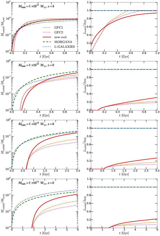
Figure 2: Cooling histories for static haloes, measured from the time when radiative cooling is turned on. The different line styles show the predictions for different cooling models, as labelled in the line key. Each row corresponds to a different halo mass and assembly redshift, as labelled. Left column: the ratio of cooled mass to total baryon mass. Right column: the ratio of the specific angular momentum of the cooled gas to the specific angular momentum of the halo. Note the different time spans in the different panels.

Fig. 2 shows the total mass and the specific angular momentum of the gas that has cooled down and accreted onto the central galaxy, as predicted by the different cooling models. Results are plotted against the time, $t$, since radiative cooling is turned on in the halo. For the fast cooling halo ($M_{\rm halo}=10^{11}\,{\rm M}_{\odot}$), all cooling models predict very similar results for the two quantities. This is because in the fast cooling regime, the accretion of the cooled down gas is mainly limited by the timescale for free-fall rather than that for radiative cooling, and all of the cooling models calculate the free-fall accretion rate in a similar way. For the more massive haloes ($M_{\rm halo}=10^{12}-10^{14}\,{\rm M}_{\odot}$), the results for the l-galaxies and morgana cooling models remain very similar, but the results for the GFC1, GFC2 and new cooling models diverge from those models and from each other.

For haloes of all masses, gas starts to accrete onto the central galaxy from $t=0$ in the l-galaxies and morgana cooling models; for the GFC1, GFC2 and new cooling models there is a time delay that varies with halo mass. This time delay is equal to the central radiative cooling timescale, $t_{\rm cool}(r=0)$. It is a consequence of the assumption that the hot gas density decreases monotonically with radius, so that $t_{\rm cool}\propto\rho_{\rm hot}(r)^{-1}$ increases with radius. In the galform cooling models, the hot gas density at $r=0$ is finite, and gas cools shell by shell, so no gas can cool and accrete before the gas at the centre cools. In contrast, in the l-galaxies cooling model, the hot gas density at $r=0$ is infinite, while in morgana, the gas does not cool shell by shell, so there is no time delay.

For the Milky Way like halo, the GFC1 and GFC2 models generally predict lower accreted masses than the new cooling model, and this difference grows with halo mass. For the $10^{14}\,{\rm M}_{\odot}$ halo, the difference can be a factor $\gtrsim 4$. The origin of this difference can be understood by looking at the cooling in more detail, as is done in Fig. 3. For conciseness, we only show the most massive halo, where the abovementioned difference is largest. The results for less massive haloes are similar.

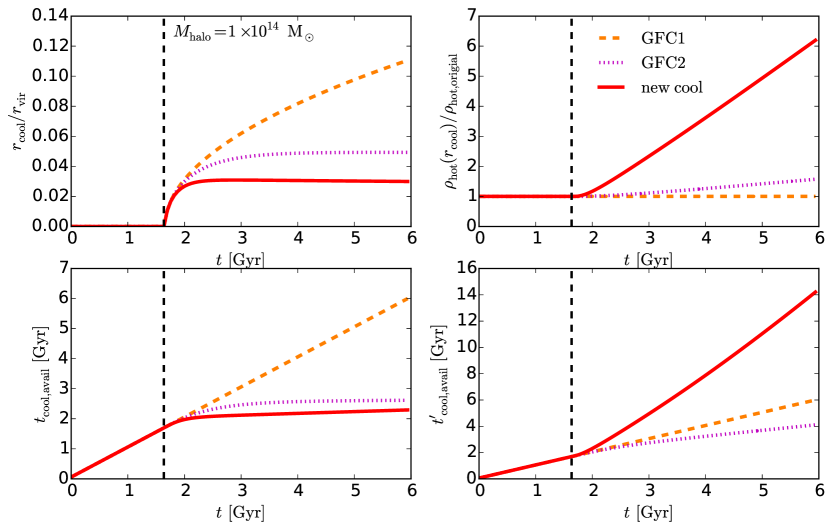
Figure 3: More detailed information on the cooling in static haloes in the three galform cooling models for $M_{\rm halo}=10^{14}\,{\rm M}_{\odot}$. From upper left to lower right, these four panels respectively show the time evolution of the cooling radius, $r_{\rm cool}$, ratio of the density of the shell at $r_{\rm cool}$ to the density of the same Lagrangian shell at $t=0$, the time available for cooling, $t_{\rm cool,avail}$, and the scaled time available for cooling, $t^{\prime}_{\rm cool,avail}$, predicted by the three models. Each line style corresponds to a different model, with the model name given in the key in the upper right panel. The vertical dashed line in each panel indicates the moment at which cooling starts.

The upper left panel of Fig. 3 shows the time evolution of the cooling radius, $r_{\rm cool}$. The GFC1 model predicts that $r_{\rm cool}$ increases monotonically with time. This is expected for a fixed hot gas halo, in which the hot gas cools down at larger and larger radii with increasing time. For the GFC2 and new cooling models, however, $r_{\rm cool}$ tends to reach a stable value instead of increasing with time. This is caused by the contraction of the hot gas halo included in these two models. Although radiative cooling leads to an increase of $r_{\rm cool}$, just as in the GFC1 model, the contraction moves the hot gas shells to smaller radii, and the competition of these two factors results in $r_{\rm cool}$ approaching a nearly constant value. The GFC2 model predicts larger values of $r_{\rm cool}$ than the new cooling model, because, as mentioned in §2.2.2, these two models adopt different contraction time scales, and the GFC2 model tends to overestimate the contraction timescale, leading to slower contraction, and resulting in values of $r_{\rm cool}$ intermediate between the GFC1 and new cooling models.

When a hot gas shell moves to smaller radius, it is compressed to a higher density. This effect is shown in the upper right panel of Fig. 3. This panel gives the ratio of the density of the gas at $r_{\rm cool}$ to the density, $\rho_{\rm hot,original}$, in the same Lagrangian gas shell at $t=0$. This ratio is always $1$ for the GFC1 model, because it assumes a static hot gas halo, while for the GFC2 and new cooling models it is larger than $1$, due to the compression induced by the hot halo contraction.

The lower left panel of Fig. 3 shows the $t_{\rm cool,avail}$ predicted by the three models. The prediction of the GFC1 model is just the physical time, while those of the GFC2 and new cooling models tend to level off at constant values. $t_{\rm cool,avail}$ encodes the previous cooling history of the hot gas. The advance of cooling tends to increase $t_{\rm cool,avail}$ by increasing $E_{\rm cool}$ in equation (13), while the hot gas halo contraction in the GFC2 and new cooling models increases the shell density, which leads to an increase of the cooling rate, and so tends to reduce $t_{\rm cool,avail}$ by increasing $L_{\rm cool}$ in equation (13). The combination of these two effects causes $t_{\rm cool,avail}$ to approach a roughly stable value.

In the GFC2 and the new cooling models $t_{\rm cool,avail}$ is used to calculate the cooled mass for the hot gas halo after contraction. As shown in the upper right panel of Fig. 3, the extent of contraction is different in these two models, while the GFC1 model does not have this contraction. Thus, the $t_{\rm cool,avail}$ in these three models are for different hot gas haloes. This makes it complicated to analyze the origin of the differences in predicted cool mass based on $t_{\rm cool,avail}$. Therefore, we introduce another quantity, $t^{\prime}_{\rm cool,avail}$, which is defined as

$$t^{\prime}_{\rm cool,avail}=t_{\rm cool,avail}\frac{\rho_{\rm hot}(r_{\rm cool})}{\rho_{\rm hot,original}},$$ (47)

where $\rho_{\rm hot}(r_{\rm cool})$ is the density of the shell that has just cooled down, while $\rho_{\rm hot,original}$ is the density at $t=0$ of the same Lagrangian shell, and this density ratio is that shown in the upper right panel of Fig. 3. Since for the shell just cooled down one has $t_{\rm cool,avail}=t_{\rm cool}(r_{\rm cool})$, and from equation (6), $t_{\rm cool}\propto\rho_{\rm hot}^{-1}$, equation (47) implies that

$$t^{\prime}_{\rm cool,avail} = t_{\rm cool}(r_{\rm cool})\frac{\rho_{\rm hot}(r_{\rm cool})}{\rho_{\rm hot,original}}$$ (48)

$$= t_{\rm cool,original},$$

where $t_{\rm cool,original}$ is the cooling timescale of this Lagrangian shell at $t=0$. Then it is clear that $t^{\prime}_{\rm cool,avail}$ is linked to the cooling timescale at the initial moment, at which the hot gas halo is the same in all three models, and so is easier to compare between models.

The lower right panel of Fig. 3 shows the $t^{\prime}_{\rm cool,avail}$ predicted by the three models. The new cooling model predicts the highest $t^{\prime}_{\rm cool,avail}$, which means that at any given time, the shell at $r_{\rm cool}$ in this model has the largest initial radius among the three models, and since at $t=0$ the hot gas halo density profile is the same for these three models, the largest radius implies the highest cooled mass. In contrast, the GFC2 model predicts the smallest $t^{\prime}_{\rm cool,avail}$, so it predicts the lowest cool mass (see Fig. 2).

The density enhancement ($\rho_{\rm hot}(r_{\rm cool})/\rho_{\rm hot,original}>1$) seen in the GFC2 and new cooling models implies a higher cooling luminosity than for the case of a fixed hot gas halo as in the GFC1 model. This higher cooling luminosity means more thermal energy is radiated away by a given time, and since the hot gas haloes in these three models all have the same temperature, this higher thermal energy loss should mean higher cooled mass. Therefore, it would be expected that for a cooling model with density enhancement, its predicted cooled mass should be higher than for a model assuming a fixed hot gas halo. Also, a higher cooled mass means the shell cooled down was initially at larger radius, and since the density decreases with increasing radius for the assumed initial density profile, this larger radius implies lower initial density and longer original cooling timescale, $t_{\rm cool,original}$. Therefore, for a given $\rho_{\rm hot}(r_{\rm cool})/\rho_{\rm hot,original}$, insofar as this ratio is greater than one, the expected $t^{\prime}_{\rm cool,avail}$ should be larger than in a model with a fixed hot gas halo, i.e. the GFC1 model.

The new cooling model does predict cooled mass and $t^{\prime}_{\rm cool,avail}$ larger than those in the GFC1 model, but the GFC2 model predicts these to be lower than in the GFC1 model, which contradicts the physical expectation above. Thus, the GFC2 model appears to be physically inconsistent, and the $t^{\prime}_{\rm cool,avail}$ in it tends to be too small. Furthermore, because $t^{\prime}_{\rm cool,avail}$ and $t_{\rm cool,avail}$ are related by the density ratio through equation (47), for a given density ratio, the underestimation of $t^{\prime}_{\rm cool,avail}$ also implies an underestimation of $t_{\rm cool,avail}$.

To understand why $t_{\rm cool,avail}$ is underestimated in the GFC2 model, consider the following. As described in §2.2.2, the GFC2 model accumulates the total energy radiated away for the current hot gas halo (equation 40) and then divides it by the current halo cooling luminosity to estimate $t_{\rm cool,avail}$. When some gas cools down from the hot gas halo, its contribution to the total energy radiated away should be removed, because this gas is no longer part of the hot gas halo, and this is the motivation for the second term in equation (40). This term basically removes the total thermal energy corresponding to the mass removed from the hot gas halo. This would be correct if the GFC2 model exactly accumulated the total energy radiated away by cooling. However, the GFC2 model adopts a very rough approximation (equation 38), whereby the cooling luminosity of a gas shell is approximated as $\delta L_{\rm cool}=4\pi\tilde{\Lambda}\rho^{2}_{\rm hot}(r)r^{2}dr\approx 4\pi\tilde{\Lambda}\bar{\rho}_{\rm hot}\rho_{\rm hot}(r)r^{2}dr$, with $\tilde{\Lambda}$ being the cooling function and $\bar{\rho}_{\rm hot}$ the mean density of the hot gas. For the $\beta$-distribution used for the static halo comparison, $\bar{\rho}_{\rm hot}\sim\rho_{\rm hot}(r=0.5r_{\rm vir})$, and for the group and cluster haloes, cooling happens in the region where $\rho_{\rm hot}(r)>\bar{\rho}_{\rm hot}$. Thus, the approximation underestimates the energy radiated away, and so the second term in equation (40) removes more energy than necessary, leading to an underestimation of $t_{\rm cool,avail}$. The final cooling depends on the relative strength of this underestimation and the density enhancement. For the static halo, this underestimation of $t_{\rm cool,avail}$ exceeds the effects of the density enhancement and leads to even less gas cooling down than in the GFC1 model, but for other cases, the results could be different.

Overall, the introduction of the contraction of the hot gas halo in the new cooling model results in more efficient cooling than in the more traditional galform cooling model GFC1. Some previous works (De Lucia et al., 2010; Monaco et al., 2014) also noticed that the GFC1 model tends to predict less gas cooling than other cooling models such as morgana and l-galaxies, and also less than SPH hydrodynamical simulations. These works suggested using more centrally concentrated hot gas density profiles such as the singular isothermal profile to bring semi-analytic predictions into better agreement with SPH simulations. However, the results here suggest that at least part of the reason for the GFC1 model giving low cooling rates is that it does not include contraction of the hot gas halo as cooling proceeds. Note that the enhancement of hot gas density and hence cooling induced by contraction is also mentioned in morgana papers (e.g. Viola et al., 2008), but taking the average over all hot gas shells to calculate the mass cooling rate (as is done in the morgana cooling model) may not be the best way to model this effect.

Fig. 2 also shows that for the haloes other than the fast cooling halo, the different cooling models predict different specific angular momenta for the gas in the central galaxies. The l-galaxies and morgana cooling models give higher specific angular momentum than the GFC1, GFC2 and new cooling models. They predict higher specific angular momentum mainly because they (implicitly) assume specific angular momentum distributions of the hot gas, $j_{\rm hot}(r)$, that are very different from the three galform models. The l-galaxies cooling model assumes that the gas accreting in the current timestep has specific angular momentum equal to the mean specific angular momentum of the dark matter halo. This corresponds to $j_{\rm hot}(r)={\rm constant}$, i.e. no dependence on the radius from which the gas is cooling. The morgana cooling model instead assumes that the mean specific angular momentum of all the gas that has cooled down and accreted onto the central galaxy over its past history is equal to the mean specific angular momentum of the current dark matter halo. In the static halo case, in which the mean specific angular momentum of the halo does not change with time, the assumption in the morgana model is equivalent to that in l-galaxies cooling model. As shown in the right column of Fig. 2, this results in the mean specific angular momentum of the cold gas in central galaxies being equal to the mean halo specific angular momentum at all times for these two models, in the case of a static halo.

In contrast, the GFC1, GFC2 and new cooling models assume that $j_{\rm hot}(r)$ increases with radius, and that the mean specific angular momentum of all the baryons in a halo is equal to the mean specific angular momentum of the halo. Under this assumption, the hot gas in the central region has lower specific angular momentum than the mean for the halo. For the haloes other than the fast cooling halo, typically only part of the hot gas cools down, and since the cooling proceeds from halo center outwards, the hot gas having low specific angular momentum cools first, so the predicted mean specific angular momentum of the cold gas in central galaxies is lower than that of the dark matter halo. The new cooling model predicts higher specific angular momentum for the cooled gas in central galaxies compared to the GFC1 and GFC2 models, because it cools more effectively, and so can cool gas shells that were originally at larger radii, which, according to the assumed $j_{\rm hot}(r)$, have higher specific angular momentum.

3.2 Cosmologically evolving haloes

Having understood the behaviours of the different cooling models in the simplified case of static haloes, the next step is to compare them in the context of cosmic structure formation. To achieve this, we run the cooling models in cosmologically evolving haloes, whose formation histories are described by merger trees. As before, we choose 4 different halo masses at $z=0$, namely $M_{\rm halo}=10^{11},\ 10^{12},\ 10^{13}$ and $10^{14}\,{\rm M}_{\odot}$. For each of these masses, we generate $100$ independent merger trees to sample the range of formation histories, using the Monte Carlo method of Parkinson et al. (2008) that is based on the Extended Press-Schechter approach (e.g. Lacey & Cole, 1993). ( We use Monte Carlo rather than N-body merger trees for this comparison because it is then easier to build equal size samples for different $z=0$ halo masses.) The merger trees are built with halo mass resolution, $M_{\rm res}=5\times 10^{9}\,{\rm M}_{\odot}$. We choose this relatively high $M_{\rm res}$ mainly to avoid too much cooling in small haloes, which would leave little gas for the slow cooling regime in high mass haloes. Star formation, SN and AGN feedback processes and galaxy mergers are all turned off in order to isolate the effects of the different cooling models. For each merger tree, the mass and angular momentum of the gas cooled and accreted onto the central galaxy in the haloes in the major branch of this merger tree are recorded.

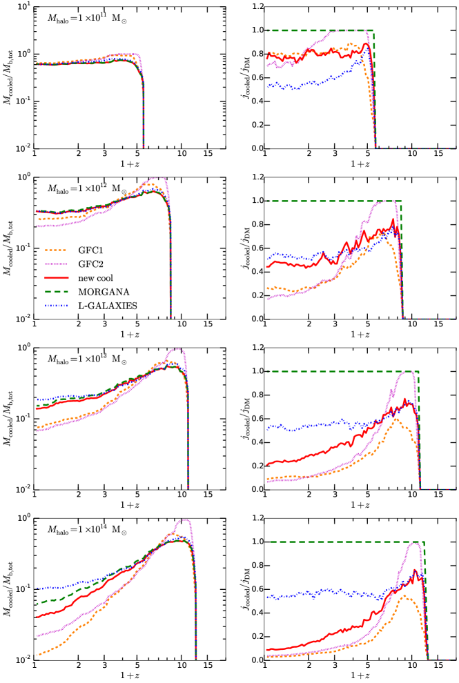
Figure 4: The same as Fig. 2, but for cosmologically evolving haloes. For each $z=0$ halo mass shown in the figure, $100$ merger trees are constructed, and the cooling models run on all branches of each merger tree. Star formation, SN and AGN feedback, and galaxy mergers are turned off. The results are recorded for the main branch of each merger tree, and the medians of each halo sample are plotted.

Fig. 4 shows the medians of $100$ realizations for each halo mass of the mass and specific angular momentum of gas accreted onto the central galaxy in the main branch of the merger tree. Many features seen in the static halo case also appear here. For the fast cooling haloes ($M_{\rm halo}=10^{11}\,{\rm M}_{\odot}$ at $z=0$), the predictions of the different cooling models are similar, again because in the fast cooling regime the accretion of gas onto galaxies is limited by the free-fall timescale and largely insensitive to the details of the cooling calculation. For the slower-cooling haloes ($M_{\rm halo}\geq 10^{12}\,{\rm M}_{\odot}$), the new cooling model predicts larger cooling masses than the GFC1 and GFC2 models, because of the contraction of the hot gas halo. For haloes less massive than $10^{14}\,{\rm M}_{\odot}$, the predictions of the new cooling model for the mass cooled down are close to those of the l-galaxies and morgana cooling models, but for $10^{14}\,{\rm M}_{\odot}$ haloes, the predictions of the new cooling model at $z=0$ are about a factor of $2$ lower than those of morgana, and a factor of $3$ lower than those of l-galaxies.

In the static halo case, the cooled down mass predicted by the GFC2 model is always lower than that of the GFC1 model, but here the relation of their predictions is more complex. For some halo masses, the GFC2 model gives higher cooled down masses, but for other halo masses, its predictions are lower. This is because the diverse halo merger histories affect the comparative strengths of the underestimation of $t_{\rm cool,avail}$ and the enhancement of the hot gas density in the GFC2 model, and the competition of these two factors determines the final cooling efficiency of this model, as described in §3.1.

The morgana cooling model forces the specific angular momentum of the cooled down gas to always equal the mean specific angular momentum of the halo by construction. Although the l-galaxies cooling model makes the same prediction in the static halo case, for dynamically evolving haloes, the l-galaxies cooling model predicts lower specific angular momenta. This is because l-galaxies assumes that the gas currently cooling and accreting onto the central galaxy has specific angular momentum equal to that of the current halo. For cosmologically evolving haloes, the halo specific angular momentum typically increases as the halo grows, so the gas cooled at earlier times tends to have lower specific angular momentum, and so the total mean specific angular momentum of all of the gas that has cooled up to that time is lower than the mean value of the current halo.

The new cooling model tends to give higher specific angular momentum than the GFC1 and GFC2 models, mainly because the new cooling model can cool gas that was originally at larger radii, which according to the assumed $j_{\rm hot}(r)$ has higher specific angular momentum.

For the dynamical halo case, a new phenomenon is that for haloes with $M_{\rm halo}\gtrsim 10^{12}\,{\rm M}_{\odot}$ at $z=0$, the GFC1, GFC2 and new cooling models predict lower specific angular momentum for the cooled down gas at $z=0$ than the l-galaxies cooling model, while for haloes with $M_{\rm halo}\lesssim 10^{12}\,{\rm M}_{\odot}$ at $z=0$, the reverse is true. This can be understood as follows:

In the absence of cooling, all four models would predict that the mean specific angular momentum of the hot gas always equals that of the dark matter halo. Typically the specific angular momentum of the dark matter halo increases as it grows, which means that the specific angular momentum of gas accreting later is higher than that of gas accreting earlier. In the presence of cooling, the gas that accreted earlier is more likely to cool, so the mean specific angular momentum of the remaining gas is higher than that of the dark matter halo.

For slower-cooling haloes (those with $M_{\rm halo}\gtrsim 10^{12}\,{\rm M}_{\odot}$ at $z=0$), typically only a small fraction of the hot gas halo cools down, so the mean specific angular momentum of the hot gas cannot be much different from that of the dark matter halo. Moreover, the cooling in this case typically happens at small radii, and because the GFC1, GFC2 and new cooling models all assume $j_{\rm hot}(r)$ increases with $r$, they predict that the gas that is currently cooling has lower specific angular momentum than the dark matter halo, and so also lower than the predictions of the l-galaxies cooling model.

For the faster cooling haloes (those with $M_{\rm halo}\lesssim 10^{12}\,{\rm M}_{\odot}$ at $z=0$), most of the gas cools, so the specific angular momentum of the remaining hot gas can end up being significantly larger than that of the halo. Since the gas ends up cooling from large radii, the specific angular momentum of the gas that cools in a single timestep may be larger than the mean for the dark halo. This effect is more or less captured in the GFC1, GFC2 and new cooling models, but not in the l-galaxies cooling model, which is why for this case l-galaxies predicts lower specific angular momentum for the cooled down gas as a whole compared to the galform cooling models.

3.3 Full galaxy formation model

In this section we show the effects of implementing the new cooling model in a full galaxy formation model. The galform, l-galaxies and morgana semi-analytic models have very different modeling of galaxy sizes, star formation, black hole growth and SN and AGN feedback. A full comparison of these models is not the aim of this paper, so here we restrict our scope to the galform model, and investigate the effects of the new cooling model on a recent version of galform, namely ‘Lacey16’ (Lacey et al., 2016). The ‘Lacey16’ model is calibrated primarily on eight observational constraints: at $z=0$, the $b_{\rm J}$ and $K$ band galaxy luminosity functions; the HI mass function; the morphological fractions; the black hole - bulge mass relation; in the range $z=0-3$, the evolution of the $K$ band galaxy luminosity function; the sub-mm galaxy number counts and redshift distributions; the far-IR number counts; and at higher redshift still, the far-UV luminosity functions of Lyman-break galaxies. As previously mentioned, the ‘Lacey16’ model adopts the GFC1 model for gas cooling in haloes.

In our comparison, we focus on three important galaxy properties. The first is the galaxy luminosity function (LF) at $z=0$. This gives the abundance of galaxies of different masses, and reproducing the observed LFs is typically a basic requirement for any successful galaxy formation model. The second is the halo mass - stellar mass/total galaxy mass (stars + cold gas) correlations at $z=0$, which are also basic propertities. The third is the galaxy size-luminosity relation. This is of special interest because the new cooling model predicts specific angular momenta for galaxies that are significantly different from previous cooling models.

We first compare the original ‘Lacey16’ model to variants using the new cooling model, while keeping the other parameters fixed at their original values. In the original ‘Lacey16’ model, as in earlier published galform models using the GFC1 cooling model, the halo virial velocity, $V_{\rm vir}$, is updated only at halo formation events, while in the new cooling model $V_{\rm vir}$ is normally updated at every timestep. Changing how $V_{\rm vir}$ is updated by itself results in significant changes in some galform predictions. To separate more clearly the effects of the new cooling model from the effects of how $V_{\rm vir}$ is updated, we define several variants which we then compare: ‘Lacey16+cv’, which is identical to the original ‘Lacey16’ model except that $V_{\rm vir}$ is updated at every timestep; ‘Lacey16+new cool’, which is the ‘Lacey16’ model with the new cooling model except with $V_{\rm vir}$ updated at formation events; and ‘Lacey16+cv+new cool’ model, which is the ‘Lacey16’ model with the new cooling model and with $V_{\rm vir}$ updated at every timestep (the default case for the new cooling model). These variants are discussed in §3.3.1.

As shown below, the ‘Lacey16+cv+new cool’ model without retuning does not provide a good match to the observed galaxy luminosity functions at $z=0$, so we then introduce a retuned model, ‘Lacey16+cv+new cool + retuned’, in which some of the other galform parameters are adjusted to provide a better fit to these data. This retuned model is discussed in §3.3.2. For simplicity, the retuning here is limited, and only considers the $z=0$ $b_{\rm J}$ and $K$ band luminosity functions and the $z=0$ morphological fractions as constraints. This retuning also tries to maintain the improvement in early-type galaxy sizes achieved by the ‘Lacey16+cv+new cool’ model.

All of these models are run on merger trees extracted from Millennium-WMAP7 N-body simulation. More details of these merger trees are given in Lacey et al. (2016).

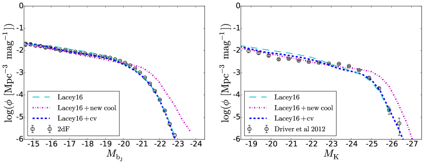
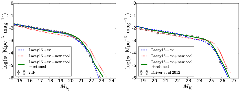
Figure 5: The galaxy luminosity functions at $z=0$ in the $b_{\rm J}$ and $K$ bands for different variants of the ‘Lacey16’ model. Each line shows the prediction for a different model, with the corresponding model name given in the key. The different models are described in the text. The top panels show the original ‘Lacey16’ model and the separate effects of changing to the new cooling model or of updating the halo virial velocity at every timestep. In the bottom panels all models have the halo virial velocity updated at every timestep. These panels include the retuned ‘Lacey16’ model incorporating the new treatment of gas cooling. The gray open circles with error bars are observational data, from Norberg et al. (2002) for the $b_{\rm J}$-band, and from Driver et al. (2012) for the $K$-band.

3.3.1 Original Lacey16 model and variations

We first consider galaxy luminosity functions (LFs). The intrinsic luminosity of a given galaxy is calculated self-consistently by convolving its star formation history with the luminosities of single stellar populations, while the extinction is calculated self-consistently based on the galaxy’s cold gas mass and metallicity and its radius. More details are given in Lacey et al. (2016). Fig. 5 shows the present-day $b_{\rm J}$- and $K$-band luminosity functions predicted by the different model variants described above, compared with observational data. The original ‘Lacey16’ model was calibrated to provide a good fit to the observed LFs. Updating the halo virial velocity, $V_{\rm vir}$, at every timestep, as for the variant ‘Lacey16+cv’, is seen by itself to produce only small changes in the LFs, reducing them slightly at the faint end. However, replacing the original cooling model (GFC1) with the new cooling model is seen to produce a large increase in the number of bright galaxies, although this effect is smaller in the model ‘Lacey16+cv+new cool’ where $V_{\rm vir}$ is updated at every timestep (lower panels), compared to the model ‘Lacey16+new cool’ where it is only updated at formation events (upper panels). In the ‘Lacey16’ model, the bright ends of the LFs at $z=0$ are controlled mainly by AGN feedback. The excesses seen at the bright ends show that the AGN feedback is too weak when the new cooling model is introduced without adjusting any other parameters. There are two reasons for this. Firstly, as shown in §3.1 and 3.2, by more carefully modeling the contraction of the hot gaseous halo, the new cooling model predicts higher cooling luminosity and more efficient cooling, which requires stronger AGN feedback to balance it. Secondly, the efficiency of the AGN feedback that is available in the model is tightly correlated with the growth of supermassive black holes (SMBH) at the centres of galaxies. As discussed in Lacey et al. (2016), in the ‘Lacey16’ model, the black hole accretion triggered by bar instabilities in galaxy disks is a major contributor to black hole growth. The new cooling model generally predicts higher angular momentum for the cooled down gas, resulting in larger disk sizes, and delaying the onset of disk instabilities (typically by $\sim 5\,{\rm Gyr}$). This then delays the onset of efficient AGN feedback, leading to ineffective AGN feedback over most of the history of a galaxy.

A further effect of using the new cooling model that is apparent in Fig. 5 is to lower the faint ends of the LFs relative to the corresponding models using the GFC1 cooling model. However, this change is fairly modest, less than a factor of $2$. This difference indicates that the new cooling model predicts less gas cooling in the haloes forming these faint galaxies, which are typically low mass ($M_{\rm halo}\lesssim 10^{12}\,{\rm M}_{\odot}$) and close to the fast cooling regime. At first sight, this seems to contradict the conclusions in §3.1 and 3.2, which claim that the cooling in low mass haloes predicted by the different cooling models is similar. However, the models used in §3.1 and 3.2 do not include SN feedback and so there is no reincorporation of the gas ejected out of the halo by SN feedback. In the full model here, this ejected gas plays a central role in gas cooling because faint galaxies have very strong SN feedback, and so a large fraction of their gas is ejected and later reaccreted.

Both the new cooling model and the GFC1 model assume that the ejected gas is gradually reincorporated into the hot gas halo, and when it joins the hot gas halo, it is shock heated to $T_{\rm vir}$, so that it joins as hot gas without any previous cooling history. However, as mentioned in §2.2.1, the GFC1 model always calculates $t_{\rm cool,avail}$ as the time since the last halo formation event, which means that ejected gas that is reincorporated between two halo formation events is treated as having been cooling for longer than it has been part of the hot halo. In contrast, the new cooling model estimates the cooling history by accumulating the energy previously radiated away, $E_{\rm cool}$, and the reincorporation of the ejected gas does not change $E_{\rm cool}$. This difference in the treatment of the reincorporated gas causes the new cooling model to predict less cooling in these low mass haloes. The strength of this effect depends on the amount of gas ejected, so only the galaxies experiencing strong SN feedback are strongly affected.

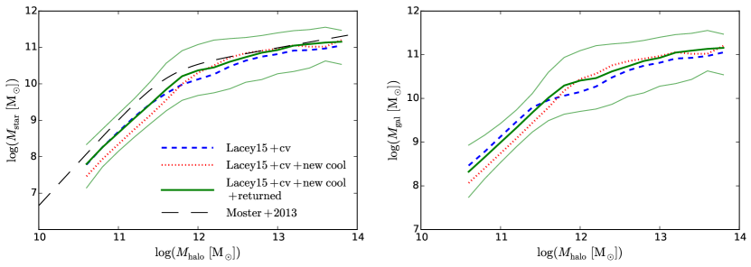
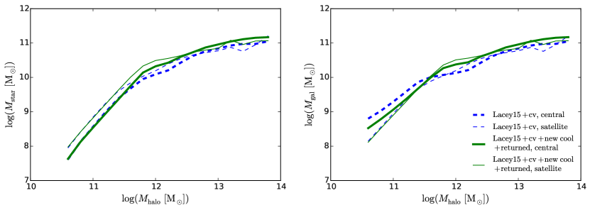
Figure 6: Upper left panel: The halo mass - stellar mass correlations at $z=0$ predicted by different models. For central galaxies, the halo masses are their host halo masses at $z=0$, while for satellites, the halo masses are the masses of haloes at infall. The thick lines of different styles are median stellar masses at a given halo mass predicted by different models, with the corresponding model names given in the key. The thin solid lines show the $5{\rm th}-95{\rm th}$ percentiles of stellar mass in the retuned model, indicating the scatter around the median correlation. The scatters in other models’ predictions are similar to the retuned model, and they are omitted here for clarity. The long dashed line indicates the correlation in Moster et al. (2013) for reference. It is derived by using an abundance matching method. Upper right panel: Similar to the upper left panel, but for the halo mass - total galaxy mass correlations at $z=0$ predicted by different models. Here the total galaxy mass is the sum of the stellar mass and the cold gas mass. Lower left panel: The halo mass - stellar mass correlations at $z=0$ predicted by different models, shown separately for central and satellite galaxies. The dashed lines show the median stellar masses for a given halo mass predicted by the ‘Lacey16+cv’ model, while the solid lines are the predictions of the retuned model. The thick lines are for the central galaxies, and the thin lines are for the satellites. The scatters around the median correlations are similar in each model’s predictions and similar to those shown in the upper two panels. They are omitted here for clarity. Lower right panel: similar to the lower left panel, but for the halo mass - total galaxy mass correlations at $z=0$.

The top row of Fig. 6 shows the halo mass - stellar mass/total galaxy mass (stars + cold gas) correlations predicted by different models. Here, for conciseness, we only show the results of models in which $V_{\rm vir}$ is updated at every timestep. With the new cooling model, i.e. in the ‘Lacey16+cv+new cool’ model, the galaxies in haloes with $M_{\rm halo}\lesssim 10^{12}\,{\rm M}_{\odot}$ tend to have lower stellar masses and total galaxy masses, which is again caused by the reduction of cooling in the new cooling model when including the reincorporated gas.

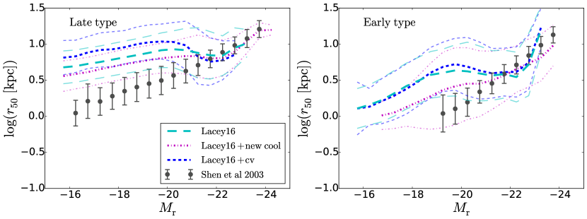
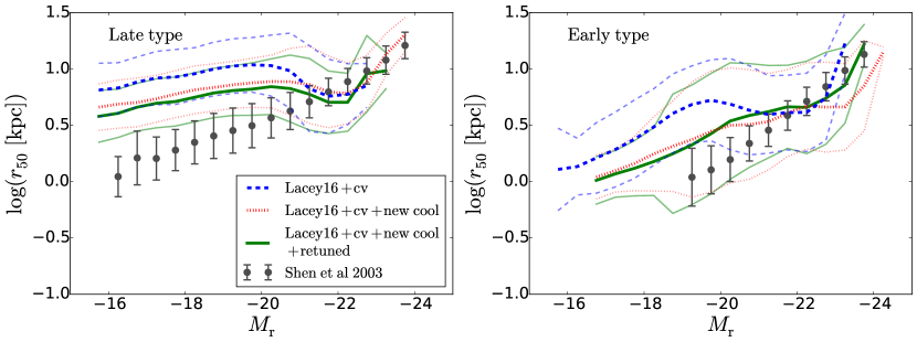
Figure 7: Half-light radii of late-type (left column) and early-type (right column) galaxies vs. luminosity at $z=0$ . Both the half-light radius and luminosity are in the $r$-band. The models plotted and their arrangement between top and bottom rows are the same as in Fig. 5. The thick lines show the median relations, while the corresponding thin lines indicate the 10-90% ranges around this. In the models, galaxies are defined as late- or early-type according to their $r$-band bulge to total ratio, $(B/T)_{r}$, with $(B/T)_{r}<0.5$ for late-type and $(B/T)_{r}>0.5$ for early-type. The gray dots with errorbars show medians and 10-90% ranges based on observational data from Shen et al. (2003). Shen et al. (2003) measured the half-light radii by fitting Sersic profiles to galaxy images and defined the late-type and early-type galaxies by Sersic index $n<2.5$ and $n>2,5$ respectively. The observed late-type galaxy sizes have been multiplied by $1.34$ to make an average correction to face-on values (see §4.3.2 of Lacey et al. (2016) for more details).

We now consider galaxy sizes. In galform, the disk size is related to the disk specific angular momentum, while the bulge size at formation is estimated based on energy conservation and the virial theorem, and these sizes are then adjusted adiabatically until the disk and bulge reach equilibrium under the gravity of each other and the halo. More details of the size calculation are given in Cole et al. (2000). Fig. 7 shows the $r$-band half-light radius vs. $r$-band absolute magnitude relations for both late-type and early-type galaxies at $z=0$. The original ‘Lacey16’ model predicts too large sizes for faint late-type galaxies ($M_{\rm r}\gtrsim-20$) and for faint early-type galaxies $V_{\rm vir}$ ($M_{\rm r}\gtrsim-21$). The ‘Lacey16+cv’ model, in which $V_{\rm vir}$ is updated at every timestep, gives similar results, with the predicted sizes of faint late-type galaxies being even larger. Using the new cooling model, as in ‘Lacey16+cv+new cool’, then reduces the sizes of faint late-type galaxies compared to the ‘Lacey16+cv’ model, due to the reduction of gas cooling when including the reincorporated gas. Lower cooled down mass implies that gas has cooled from smaller radii in the hot gas halo, because the cooling proceeds from the halo center outwards. Then, since in galform the assumed hot gas specific angular momentum distribution predicts lower specific angular momentum at smaller radii, the reduction of cooling leads to the reduction of galaxy specific angular momenta and thus galaxy sizes. However, the sizes of late type galaxies in the ‘Lacey16+cv+new cool’ model are almost the same when compared to the original ‘Lacey16’ model. This indicates that some physical effect other than gas cooling in haloes must be responsible for the deviation of the model prediction from observations for late-type galaxies. One possibility is that the current galform model assumes the same radius for both stellar and gas disks in a galaxy. In reality, the gas disk could be more extended than the stellar disk, because star formation happens mainly in the central region of the gas disk, where the gas density is higher.

Using the new cooling model results in a larger improvement in the size-luminosity correlation of the early-type galaxies at $z=0$. The predicted relation is now in better agreement with observations, much better than both the original ‘Lacey16’ and ‘Lacey16+cv’ models, although the scatter around the median is still much larger than observed. This improvement is mainly due to the reduction in the sizes of the faint early-type galaxies. This can again be understood as a consequence of the reduction of cooling in relatively low mass haloes when including the reincorporated gas.

3.3.2 Retuned Lacey16 model

As already discussed, we retune some of the parameters in the version of the ‘Lacey16’ model incorporating the new cooling model, in order to match better the $z=0$ $b_{\rm J}$ and $K$-band LFs at $z=0$, using the early-type galaxy fraction at different luminosities as a secondary constraint (see §4.2.3 in Lacey et al. (2016)). At the same time, we ensure that the improvement in the size-luminosity correlation of the early-type galaxies at $z=0$ is not spoilt. The retuned parameters are summarized in Table 1.

Table 1: Retuned parameters and their original values in the ‘Lacey16’ model.

parameter	Lacey16	retuned	description
$\alpha_{\rm cool}$	$0.8$	$1.4$	threshold of the
			ratio of the free-fall/cooling
			time scale
$\gamma_{\rm SN}$	$3.2$	$2.8$	slope of the SN feedback
			power-law scaling
$f_{\rm df}$	$1.0$	$0.7$	normalization of the
			dynamical friction sinking
			time scale

To match the LF measurements, the major problem needing to be solved is the excess at the bright end. As discussed in §3.3.1, this is due to the ineffectiveness of AGN feedback, which is a combined effect of enhanced cooling and the less efficient black hole growth induced by the suppression of the disk instabilities. One direct solution would be to increase the number of disk instabilities by raising the stability threshold, which is somewhat uncertain. However, the faint early-type galaxies are mainly produced by disk instabilities, and raising the stability threshold would let disks with higher specific angular momentum, and thus larger sizes, be turned into spheroids. This would increase the median size of the faint early-type galaxies, and thus spoil the improvement achieved by using the new cooling model. Therefore other ways of enhancing the AGN feedback effect should be considered first. The effect of the AGN feedback can also be increased by turning on AGN feedback earlier. This can be done by increasing the parameter $\alpha_{\rm cool}$, which sets the threshold of the ratio of the free-fall timescale over the cooling timescale (both evaluated at $r=r_{\rm cool}$) at which AGN feedback turns on (for more details see Appendix D). Here, we increase $\alpha_{\rm cool}$ from 0.8 to 1.4.

We also slightly reduce the uncertain SN feedback strength in low-mass galaxies to improve the predictions for the faint ends of the LFs. In galform, the strength of the SN feedback scales with galaxy circular velocity, $V_{\rm c}$, as a power-law, $V_{\rm c})^{-\gamma_{\rm SN}}$. We reduce $\gamma_{\rm SN}$ from $3.2$ to $2.8$.

We also slightly reduce the also uncertain galaxy merger timescale to improve the predicted early-type fraction for bright galaxies. The original ‘Lacey16’ model and all the variations considered here adopt the fitting formula from Jiang et al. (2008) to calculate the galaxy merger timescale due to dynamical friction. We modify this by introducing an extra factor $f_{\rm df}$ in the formula for the galaxy merger timescale (equation (14) in Lacey et al. (2016)). The original fit in Jiang et al. (2008) implies $f_{\rm df}=1$, and this value was effectively assumed in Lacey et al. (2016). Here we reduce $f_{\rm df}$ to $0.7$, which is still roughly consistent with the simulation data in Jiang et al. (2008) (see their Fig. 10). The most important effect of this is to increase the number of mergers, particularly major mergers.

After this limited retuning of parameters, the predicted LFs agree with observations again, as shown in the bottom row of Fig. 5. The improvements in the predicted galaxy sizes are largely retained.

The halo mass - stellar mass/total galaxy mass correlations predicted by the retuned model are very similar to those of the ‘Lacey16+cv’ model (top row of Fig. 6). This is not very surprising, because these two models are tuned to reproduce the $K$-band LF, which is tightly related to galaxy stellar masses. The stellar and total galaxy masses in haloes with $M_{\rm halo}\lesssim 10^{12}\,{\rm M}_{\odot}$ in the retuned model are close to those in the ‘Lacey16+cv’ model because the SN feedback strength in the retuned model is reduced and more mass can stay in galaxies. We checked that in haloes with $M_{\rm halo}\lesssim 10^{12}\,{\rm M}_{\odot}$, the masses delivered to galaxies by cooling are still close to those in the model before retuning (i.e. ‘Lacey16+cv+new cool’ model) and lower than in the ‘Lacey16+cv’ model. This comfirms that when we include the reincorporated gas, the new cooling model predicts less cooling in low mass haloes.

For the retuned model as well as for the ‘Lacey16+cv’ model, we also show the halo mass - stellar mass/total galaxy mass correlations separately for central galaxies and satellites. These correlations are shown in the bottom row of Fig. 6. The differences between central and satellite galaxies are mainly in the halo mass range $M_{\rm halo}\lesssim 10^{12}\,{\rm M}_{\odot}$. In this range, for a given halo mass, the satellites tend to have higher stellar mass, but lower galaxy mass, which implies they contain less cold gas than the central galaxies. Switching from the GFC1 model to the new cooling model does not change this difference between central and satellite galaxies.

4 summary

We have introduced a new model, better motivated and more self-consistent than previous models, for gas cooling in haloes and accretion of gas onto galaxies for use in semi-analytic models of galaxy formation. In this model we explicitly calculate the contraction of the density profile of the hot gas halo induced by cooling and by dark matter halo growth. This contraction was not calculated explicitly in the previous galform cooling models, nor in the l-galaxies cooling model, while the morgana cooling model only considers the contraction of the hot gas halo induced by cooling. We include the effect of the cooling history of the hot gas on the current mass cooling rate by estimating the total energy lost by cooling over the history of the gas in the halo, using a new iterative scheme. We argue that our new method for calculating mass accretion rates onto galaxies is more accurate and more physically motivated than the other cooling models mentioned above. In the new model we also follow the evolution of the angular momentum distribution of the hot gas halo under the effects of contraction of the hot gas distribution, which enables a more detailed and self-consistent calculation of the angular momentum of the gas accreted onto galaxies.

After setting out the methodology of the new cooling model, we then compare its predictions to those of several previous cooling models, including two older galform cooling models and the cooling models in l-galaxies and morgana. The comparison is first done for static dark matter haloes with masses in the range $10^{11}-10^{14}\,{\rm M}_{\odot}$. The comparison is then done for evolving dark matter haloes with full merger histories, for haloes covering the same mass range at $z=0$. Both of these comparisons include gas cooling and accretion only, without any kind of feedback effects. Finally, we investigate the effects of our new cooling model on a full galaxy formation calculation, our starting point being the ‘Lacey16’ (Lacey et al., 2016) galform model. Using the new cooling model without any other adjustments results in too many bright galaxies, and thus spoils the bright end of the predicted galaxy luminosity functions. However, by slightly adjusting the values of three uncertain parameters relating to SN and AGN feedback and to the timescale for dynamical friction, we are able to bring the galform model predictions back into agreement with observations.

Compared to the cooling models previously used in galform, the improved calculation of the cooling history and the detailed modeling of the contraction of the hot gas halo significantly increase the mass that cools in massive haloes. Some previous works (e.g. De Lucia et al., 2010; Monaco et al., 2014) argued that the galform cooling model tends to underestimate the gas mass that cools in massive haloes, and proposed using a more centrally concentrated hot gas density profile (e.g. a singular isothermal profile) to solve this problem. However, in the new cooling model, the predicted cooled mass becomes closer to the predictions of the l-galaxies and morgana cooling models.

When comparing predictions between different cooling models for the angular momentum of the cooled down gas, even larger differences are seen than for the mass. The new cooling model tends to predict higher specific angular momentum of the cooled down gas than the cooling models previously used in galform. On the other hand, the predictions of the new cooling model for the angular momentum are generally smaller than those from the l-galaxies and morgana cooling models. This is mainly because different models adopt different distributions for the specific angular momentum of the hot gas, and different treatments of the effects of cooling on these distributions.

In the full galform model with all other processes such as star formation, supernova (SN) feedback and AGN feedback included, the new cooling model tends to predict less gas cooling in lower mass haloes ($M_{\rm halo}\lesssim 10^{12}\,{\rm M}_{\odot}$) than the cooling model previously used in galform, because it models more correctly the effects of the gas that is reincorporated into the hot gas halo after being ejected by SN feedback. This effect improves the predicted size-luminosity relation of both early-type and late-type galaxies relative to observations. However, the improvement in the sizes of late-type galaxy is very small, which indicates that other physical effects may be involved in explaining the discrepancy with observations. For example, galform forces the stellar and gas disks to have the same scale radius, while in reality, the gas disk could be much more extended than the stellar disk. The inclusion of the new cooling model into galform and the retuning of a handful of uncertain parameters (see Table 1) in the latest version of the model (‘Lacey16’) leads to an improved model, which supersedes previous versions of galform.

Having understood the behavior of the new cooling model, and having compared the new cooling model to other cooling models, the next step is to compare the predictions of the new cooling model with the results from hydrodynamical simulations. We leave this comparison for future work.

Appendix A Approximate recursive equation for $E_{\rm cool}$

Here we consider the change of $E_{\rm cool}$ in a timestep $(t,t+\Delta t]$, and derive an approximate equation that relates $E_{\rm cool}(t)$ and $E_{\rm cool}(t+\Delta t)$. This equation can then be used to calculate $E_{\rm cool}$ at any given time recursively from the initial time $t_{\rm init}$.

Within this timestep, the hot gas halo is treated as fixed, with its inner and outer boundaries respectively at $r_{\rm cool,pre}(t)$ and $r_{\rm vir}(t)$. By $t+\Delta t$, the gas between $r_{\rm cool,pre}(t)$ and $r_{\rm cool}(t+\Delta t)$ has cooled down.

From equation (12), one has

$$E_{\rm cool}(t+\Delta t)=4\pi\int_{t_{\rm init}}^{t+\Delta t}\int_{r^{\prime}_{\rm p}(\tau)}^{r_{\rm vir}(\tau)}\tilde{\Lambda}\rho_{\rm hot}^{2}(r,\tau)r^{2}drd\tau,$$ (49)

where $\tilde{\Lambda}$ is the cooling function, $\rho_{\rm hot}(r,\tau)$ is the density of the hot gas at radius $r$ and time $\tau$, and $r^{\prime}_{\rm p}(\tau)$ is the radius at $\tau$ of a shell that has radius $r_{\rm cool}$ at $t+\Delta t$. Note that here we use $r_{\rm cool}$ instead of $r_{\rm cool,pre}(t+\Delta t)$, because the hot halo is fixed here, and in the new cooling model, after the cooling calculation, the halo contraction would change $r_{\rm cool}(t+\Delta t)$ to $r_{\rm cool,pre}(t+\Delta t)$.

Then equation (49) can be further expanded as

$$E_{\rm cool}(t+\Delta t) = 4\pi\int_{t_{\rm init}}^{t+\Delta t}\int_{r_{\rm p}(\tau)}^{r_{\rm vir}(\tau)}\tilde{\Lambda}\rho_{\rm hot}^{2}(r,\tau)r^{2}drd\tau$$ (50)

$$- 4\pi\int_{t_{\rm init}}^{t+\Delta t}\int_{r_{\rm p}(\tau)}^{r^{\prime}_{\rm p}(\tau)}\tilde{\Lambda}\rho_{\rm hot}^{2}(r,\tau)r^{2}drd\tau$$

$$= I_{1}-I_{2},$$

where $I_{1}$ and $I_{2}$ represent respectively the two integrals in the above equation, and $r_{\rm p}(\tau)$ is the radius at $\tau$ of a shell that has radius $r_{\rm cool,pre}$ at $t+\Delta t$. Note that at $t+\Delta t$ the hot gas halo inner boundary is still at $r_{\rm cool,pre}(t)$ because the halo is assumed to be static over the interval $(t,t+\Delta t]$. Further

$$I_{1} = 4\pi\int_{t_{\rm init}}^{t}\int_{r_{\rm p}(\tau)}^{r_{\rm vir}(\tau)}\tilde{\Lambda}\rho_{\rm hot}^{2}(r,\tau)r^{2}drd\tau$$ (51)

$$+ 4\pi\int_{t}^{t+\Delta t}\int_{r_{\rm p}(\tau)}^{r_{\rm vir}(\tau)}\tilde{\Lambda}\rho_{\rm hot}^{2}(r,\tau)r^{2}drd\tau$$

$$= E_{\rm cool}(t)+\Delta t\times 4\pi\int_{r_{\rm cool,pre}}^{r_{\rm vir}}\tilde{\Lambda}\rho_{\rm hot}^{2}(r,t)r^{2}dr$$

$$= E_{\rm cool}(t)+L_{\rm cool}(t)\Delta t,$$

in which we have used equation (12) for the first integral in the above equation, while the second integral is simplified by the assumption that the hot gas halo is fixed within $(t,t+\Delta t]$, with the inner and outer boundaries $r_{\rm cool,pre}$ and $r_{\rm vir}$ respectively, and $L_{\rm cool}(t)$ is defined in equation (11).

$I_{2}$ can be further written as

$$I_{2} = 4\pi\int_{t}^{t+\Delta t}\int_{r_{\rm p}(\tau)}^{r^{\prime}_{\rm p}(\tau)}\tilde{\Lambda}\rho_{\rm hot}^{2}(r,\tau)r^{2}drd\tau$$ (52)

$$+ 4\pi\int_{t_{\rm init}}^{t}\int_{r_{\rm p}(\tau)}^{r^{\prime}_{\rm p}(\tau)}\tilde{\Lambda}\rho_{\rm hot}^{2}(r,\tau)r^{2}drd\tau$$

$$= L^{\prime}_{\rm cool}\Delta t+I_{3},$$

where $L^{\prime}_{\rm cool}(t)$ is defined in equation (15), and the first integral in the above equation is simplified again because the hot gas halo is assumed fixed within $(t,t+\Delta t]$, while $I_{3}$ corresponds to the second integral above.

The integral $I_{3}$ represents the total energy radiated away by the gas within $r_{\rm cool,pre}\leq r\leq r_{\rm cool}$ from $t_{\rm init}$ to $t$, and it can be rewritten as the summation of $\delta E_{\rm cool}$ of each gas shell in this range, namely

$$I_{3} = \int_{r_{\rm cool,pre}}^{r_{\rm cool}}\frac{\delta E_{\rm cool}}{\delta r}dr$$ (53)

$$= \int_{r_{\rm cool,pre}}^{r_{\rm cool}}\frac{\delta E_{\rm cool}}{\delta L_{\rm cool}}\frac{\partial L_{\rm cool}}{\partial r}dr$$

$$= \int_{r_{\rm cool,pre}}^{r_{\rm cool}}\tilde{t}_{\rm cool,avail}(r,t)\frac{\partial L_{\rm cool}}{\partial r}dr,$$

in which we derive the third line from the second line by virture of the definition of $\tilde{t}_{\rm cool,avail}$ for an individual gas shell given in equation (7).

Now consider that in the slow cooling regime, typically $r_{\rm cool}$ is close to $r_{\rm cool,pre}$, thus the radial dependence in $\tilde{t}_{\rm cool,avail}(r,t)$ can be ignored, while in the fast cooling regime, although $r_{\rm cool}$ could be much larger than $r_{\rm cool,pre}$, the cooling is so fast that halo growth and hot gas halo contraction only have weak effects on the cooling, and thus can only introduce weak dependence of $\tilde{t}_{\rm cool,avail}$ on $r$. In all, for $r_{\rm cool,pre}\leq r\leq r_{\rm cool}$, we can approximate $\tilde{t}_{\rm cool,avail}(r,t)\approx\tilde{t}_{\rm cool,avail}(r_{\rm cool},t)$, so

$$I_{3} \approx \tilde{t}_{\rm cool,avail}(r_{\rm cool},t)\int_{r_{\rm cool,pre}}^{r_{\rm cool}}\frac{\partial L_{\rm cool}}{\partial r}dr$$ (54)

$$= \tilde{t}_{\rm cool,avail}(r_{\rm cool},t)L^{\prime}_{\rm cool},$$

where $L^{\prime}_{\rm cool}(t)$ is defined in equation (15) and is the total cooling luminosity at $t$ of the gas between $r_{\rm cool,pre}\leq r\leq r_{\rm cool}$. Note that for hot gas halo that is fixed at all times, this approximation becomes exact. Based on this, one has

$$I_{2} \approx [\Delta t+\tilde{t}_{\rm cool,avail}(r_{\rm cool},t)]L^{\prime}_{\rm cool}$$ (55)

$$= \tilde{t}_{\rm cool,avail}(r_{\rm cool},t+\Delta t)L^{\prime}_{\rm cool}$$

$$\approx t_{\rm cool,avail}(t+\Delta t)L^{\prime}_{\rm cool},$$

in which we have used equations (8) and (13).

Substituting equations (51) and (55) into equation (50), one reaches the approximate recursive equation for $E_{\rm cool}$, i.e. equation (14).

Appendix B Calculation of the change in the angular momentum distribution of the hot gas halo

B.1 Approximate calculation of $j_{\rm hot}[r(r^{\prime})]$

In the new cooling model, the hot gas halo evolves with the growth of the dark matter halo, and it also contracts in response to gas cooling, which removes pressure support from the central regions. These effects change the specific angular momentum distribution of the hot gas halo. We assume that each spherical shell of hot gas conserves its specific angular momentum, $j_{\rm hot}$, during this change, but the shell moves from $r$ to $r^{\prime}$, and thus the angular momentum profile changes from $j_{\rm hot}(r)$ to $j^{\prime}_{\rm hot}(r^{\prime})=j_{\rm hot}[r(r^{\prime})]$. As described in §2.1.4, $r(r^{\prime})$ can be determined through equation (22), which is based on mass conservation for each shell. For the assumed form of the hot gas density profile, this equation does not have an explicit analytical solution, leading to no exact analytical expression for $j_{\rm hot}[r(r^{\prime})]$. While $j_{\rm hot}[r(r^{\prime})]$ can be derived numerically for each shell at every timestep, this is computationally expensive, and so here we present an approximate analytical expression that can be used instead. In Appendix B.2, we test the accuracy of this analytical approximation against a numerical solution of the same equations.

At the end of a timestep, the hot gas is distributed between $r_{\rm cool}$ and $r_{\rm vir}$, following a $\beta$-distribution with core radius, $r_{\rm core}$. Before the calculation of the next timestep, the effects of halo growth and hot gas halo contraction during the current timestep should be included. These effects redistribute the hot gas that was previously in this halo. The inner boundary of the hot gas moves from $r_{\rm cool}$ to $r_{\rm cool,pre}$, while the outer boundary moves from $r_{\rm vir}$ to $r^{\prime}_{\rm vir}$. According to the assumptions in §2.1.2, this adjusted gas still follows a $\beta$-distribution, but with a new core radius $r^{\prime}_{\rm core}$. As mentioned in §2.1.4, this adjustment is only for the hot gas previously in this halo, while the newly added hot gas is assumed to mix with the hot gas halo after this adjustment. Therefore the total gas mass, $M_{\rm hot}$, before and after this adjustment is unchanged.

When considering the approximate calculation of $j_{\rm hot}[r(r^{\prime})]$, it is more convenient to work with the variables $x\equiv r/r_{\rm core}$ and $x^{\prime}\equiv r^{\prime}/r^{\prime}_{\rm core}$ instead of $r$ and $r^{\prime}$. Then the angular momentum profile after the adjustment of the hot gas halo can be written as $j_{\rm hot}[x(x^{\prime})]$. The function $x(x^{\prime})$ can be derived from equation (22), which can be written as

$$M_{\rm hot}(<x)=M^{\prime}_{\rm hot}(<x^{\prime}),$$ (56)

where $M_{\rm hot}(<x)$ is the mass of hot gas within radius $x$ according to the density profile before the adjustment induced by hot gas halo contraction and dark matter halo growth, while $M^{\prime}_{\rm hot}(<x^{\prime})$ is the mass of hot gas within $x^{\prime}$ according to the density profile after this adjustment. As mentioned above, $x$ and $x^{\prime}$ are respectively the radii of the same Lagrangian shell before and after the adjustment. Note that at the inner boundary the above equation satisfies the condition $M_{\rm hot}(<x_{0})=M^{\prime}_{\rm hot}(<x^{\prime}_{0})=0$, where $x_{0}=r_{\rm cool}/r_{\rm core}$ and $x^{\prime}_{0}=r_{\rm cool,pre}/r^{\prime}_{\rm core}$, while at the outer boundary it satisfies $M_{\rm hot}(<x_{\rm vir})=M^{\prime}_{\rm hot}(<x^{\prime}_{\rm vir})=M_{\rm hot}$, where $x_{\rm vir}=r_{\rm vir}/r_{\rm core}$ and $x^{\prime}_{\rm vir}=r^{\prime}_{\rm vir}/r^{\prime}_{\rm core}$.

According to the assumed $\beta$-distribution, one has

$$M_{\rm hot}(<x)=\frac{M_{\rm hot}}{Y_{\rm vir}-Y_{0}}[x-\arctan(x)-Y_{0}],$$ (57)

where $Y_{\rm vir}=x_{\rm vir}-\arctan(x_{\rm vir})$ and $Y_{0}=x_{0}-\arctan(x_{0})$. Similarly, for the hot gas halo after the adjustment, one has

$$M^{\prime}_{\rm hot}(<x^{\prime})=\frac{M_{\rm hot}}{Y^{\prime}_{\rm vir}-Y^{\prime}_{0}}[x^{\prime}-\arctan(x^{\prime})-Y^{\prime}_{0}],$$ (58)

where $Y^{\prime}_{\rm vir}=x^{\prime}_{\rm vir}-\arctan(x^{\prime}_{\rm vir})$ and $Y^{\prime}_{0}=x^{\prime}_{0}-\arctan(x^{\prime}_{0})$.

Substituting equations (57) and (58) into equation (56), one derives an implicit form for the function $x(x^{\prime})$

$$x-\arctan(x) = \frac{Y_{\rm vir}-Y_{0}}{Y^{\prime}_{\rm vir}-Y^{\prime}_{0}}[x^{\prime}-\arctan(x^{\prime})]$$ (59)

$$+ \frac{Y^{\prime}_{\rm vir}Y_{0}-Y_{\rm vir}Y^{\prime}_{0}}{Y^{\prime}_{\rm vir}-Y^{\prime}_{0}}.$$

Equation (59) does not allow an explicit analytical expression for $x(x^{\prime})$. However, it is still possible to construct simple analytical approximations for $x(x^{\prime})$ in different ranges of $x^{\prime}$, and so to derive analytical approximations for $j_{\rm hot}[x(x^{\prime})]$.

First note that typically $x^{\prime}\leq x$, because the contraction moves shells from large radii to small radii. When $x^{\prime}$ is large, both $x-\arctan(x)$ and $x^{\prime}-\arctan(x^{\prime})$ can be well approximated by linear functions. These linear functions then lead to a linear functional form for $j_{\rm hot}[x(x^{\prime})]$. This linear functional form can be kept during the recursion procedure, which is necessary for deriving the specific angular momentum distribution from its initial value, so for large enough $x^{\prime}$, $j_{\rm hot}[x(x^{\prime})]$ can always be expressed as a linear function of $x^{\prime}$.

On the other hand, when $x^{\prime}$ is very close to $0$, a Taylor expansion gives $x^{\prime}-\arctan(x^{\prime})=x^{\prime 3}/3-{x^{\prime}}^{5}/5+O(x^{\prime 7})$. Note that this typically happens in the slow cooling regime, in which the cooling is limited to the central region of the halo and the induced contraction of the hot gas halo is small in each timestep, so typically in this case $x$ is also close to $0$, and the Taylor expansion is also a good approximation for $x-\arctan(x)$, i.e. $x-\arctan(x)=x^{3}/3-{x}^{5}/5+O(x^{7})$. These nonlinear terms in the Taylor expansions cause $j_{\rm hot}$ to gradually deviate from the assumed linear form before the starting of cooling. The nonlinear terms in the Taylor expansions are third and fifth order. This suggests the following expression for $j_{\rm hot}[x(x^{\prime})]$

$$j_{\rm hot}[x(x^{\prime})]=c_{1}x^{\prime 6}+c_{2}x^{\prime 5}+c_{3}x^{\prime 3}+c_{4}x^{\prime}+c_{5},$$ (60)

where $c_{1}-c_{5}$ are coefficients and we include all terms with orders lower than $O(x^{\prime 7})$ that can be generated by the third and fifth order terms, while the linear term is added to include the initial linear form of the angular momentum profile.

When $x$ (and also $x^{\prime}$) are either not very large or not close to $0$, the function $x-\arctan(x)$ has a non-linear dependence, but not so strong as in the case when $x$ is close to $0$. Thus, generally speaking, $j_{\rm hot}[x(x^{\prime})]$ in this regime can be expressed approximately as a lower order polynomial, and here we choose a second-order polynomial.

In summary, we adopt the following piecewise function as the analytical approximation for $j_{\rm hot}[x(x^{\prime})]$

$$j_{\rm hot}[x(x^{\prime})]=\left\{\begin{array}[]{lr}a_{1}x^{\prime}+a_{2},&x^{\prime}\geq 3.5\\ a_{3}x^{\prime}+a_{4},&2.0\leq x^{\prime}<3.5\\ a_{5}x^{\prime 2}+a_{6}x^{\prime}+a_{7},&0.5\leq x^{\prime}<2.0\\ a_{8}x^{\prime 6}+a_{9}x^{\prime 5}+a_{10}x^{\prime 3}&\\ +a_{11}x^{\prime}+a_{12},&0.0\leq x^{\prime}<0.5\end{array}\right.$$ (61)

where $a_{1}-a_{12}$ are coefficients, with the coefficients in equation (60) to be renamed as $a_{8}-a_{12}$.

The procedure is then as follows. At each timestep, several sample points are taken over the whole range of $x^{\prime}$, and then equation (59) is solved numerically for these sample points to find the corresponding $x$, with the specific angular momentum distribution in the last timestep, $j_{\rm hot}[x(x^{\prime})]$ being known for these sample points. Using these values, equation (61) then becomes a set of linear equations for the coefficients $a_{1}-a_{12}$, which can be solved easily. Once these coefficients are determined, then the approximate $j_{\rm hot}[r(r^{\prime})]$ can be calculated for any value of $r^{\prime}$ for the current timestep. Then the contribution from the newly added gas, $j_{\rm new}(r^{\prime})$, can be added as described in §2.1.4. Since it is assumed that $j_{\rm new}(r^{\prime})\propto r^{\prime}$, this further changes the coefficients of the first and zeroth order terms in equation (61). After this, the angular momentum profile of this timestep is fully determined.

This approximation requires $9$ sample points for determining $a_{1}-a_{12}$ (two adjacent $x^{\prime}$ sections share one common sample point), and so equation (59) needs to be solved for $x(x^{\prime})$ only $9$ times at each timestep. An alternative to this approximate method would be to evaluate $j_{\rm hot}[r(r^{\prime})]$ numerically on a radius grid, which would require solving equation (59) at each radius grid point, rather than at a handful of sample points. The approximate method is computationally much faster than the straightforward radius grid method. Also, the approximate method only requires storing the $12$ coefficients, while the radius grid method requires storing the whole radius grid and the numerical $j_{\rm hot}[r(r^{\prime})]$ on it, and thus would require much more computer memory.

B.2 Comparison with direct calculation

To assess the accuracy of the approximation introduced in the previous section, we compared the angular momentum accretion rates for central galaxies calculated using this approximation with those calculated using a direct (but more computationally intensive) calculation. This direct calculation evaluates $j_{\rm hot}(r)$ numerically on a radius grid at each timestep. The radius grid covers the range between $r_{\rm cool,pre}$ and $r_{\rm vir}$ with $1000$ grid points. $j_{\rm hot}(r)$ at a given timestep is calculated from $j_{\rm hot}(r)$ at the previous timestep by solving equation (59) for each grid point, and then using equation (25).

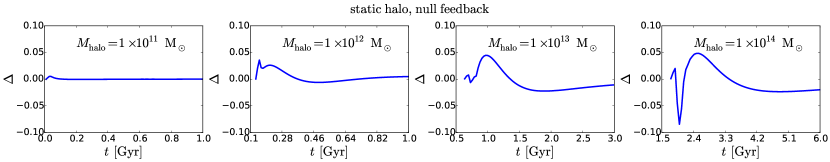
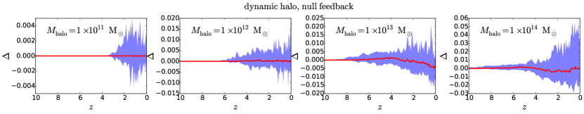
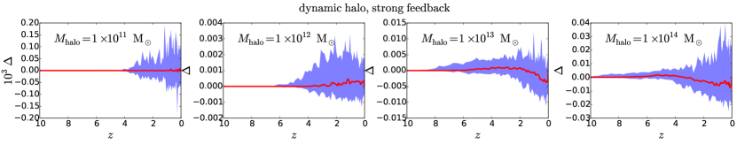
Figure 8: The relative error, $\Delta$, in the angular momentum accretion rate calculated using the approximate method for evolving $j_{\rm hot}(r)$ compared with that obtained from the direct calculation. Results are shown for 3 cases (static halo without feedback, dynamically evolving halo without feedback, and dynamically evolving halo with strong supernova feedback) and 4 different halo masses ($10^{11}$, $10^{12}$, $10^{13}$ and $10^{14}\,{\rm M}_{\odot}$). The $10^{11}\,{\rm M}_{\odot}$ static halo is at $z=3$, and other static haloes are at $z=0$, while for dynamic haloes, these masses are the halo masses at $z=0$. The dynamic halo cases use full halo merger histories, with $100$ Monte Carlo merger trees for each halo mass. For the dynamic halo cases, in each panel the solid line shows the median of the relative error, while the shaded region indicates the $5-95\%$ range. See text for more details.

The comparison is done for three cases. The first one is for static haloes, with no feedback. The second is for dynamically evolving haloes, including full halo merger histories, but still without any feedback. The third is also for dynamically evolving haloes, but with strong supernova feedback. Here the supernova feedback is modeled as usual in galform, with a mass ejection rate from the galaxy into the ejected gas reservoir $\dot{M}_{\rm eject}=\beta\psi$, where $\psi$ is the star formation rate and the mass-loading factor $\beta=(V_{\rm c}/V_{\rm SN})^{-\gamma_{\rm SN}}$, with $V_{\rm c}$ being the circular velocity of the galaxy and $V_{\rm SN}$ and $\gamma_{\rm SN}$ parameters. For the calculations here, we use $V_{\rm SN}=320\,{\rm km}\,{\rm s}^{-1}$ and $\gamma_{\rm SN}=3.2$, which are close to the values adopted in recent versions of galform. The calculations are done for four different halo masses, namely $M_{\rm halo}=10^{11},\ 10^{12},\ 10^{13}$ and $10^{14}\,{\rm M}_{\odot}$, which covers both the fast and slow cooling regimes. The $10^{11}\,{\rm M}_{\odot}$ static halo is at $z=3$, and other static haloes are at $z=0$, while for dynamic haloes, these masses are the halo masses at $z=0$. For the dynamically evolving haloes, results are calculated for $100$ Monte Carlo merger trees for each halo mass.

For each of these cases, the angular momentum accretion rate onto the central galaxy due to the cooling flow, $\dot{J}_{\rm cool}$, is calculated at each timestep, both for the approximate method in Appendix B.1 ($\dot{J}_{\rm cool,app}$) and for the direct calculation ($\dot{J}_{\rm cool,grid}$). The relative error, $\Delta$, is then calculated as $\Delta=(\dot{J}_{\rm cool,app}-\dot{J}_{\rm cool,grid})/\dot{J}_{\rm cool,grid}$. Fig. 8 shows this relative error for the three cases and the four different halo masses. From this figure, it can be seen that the relative error is generally less than $10\%$, so the approximate method works well.

Appendix C Random walk model for evolution of $\lambda_{\rm halo}$

C.1 Random walk model of halo spin evolution

The evolution of halo spin results from the angular momentum and mass brought into the halo by accretion and mergers. The angular momentum of the accreted material originates from the action of gravitational tidal torques at earlier times. This angular momentum depends on the tangential component of the infall velocity. A simple model for the halo growth is to assume that these accretion/merger events are random, with random infall velocities. In this case, the evolution of the halo spin accompanying the mass accretion is a kind of random walk (e.g. Vitvitska et al., 2002). For simplicity, we further assume that this random walk for the halo spin is a Markov walk, meaning that each step is statistically independent of previous steps.

In this picture, the spins of the descendant halo and its major progenitors are related by a conditional spin distribution, which gives the probability density for any given descendant spin value given the spin and mass accretion history of the progenitor. We now derive the form of this probability distribution for some plausible assumptions.

C.2 Conditional distribution of descendant halo spin

Mathematically, a random walk is described as a sequence of random variables, $Y(x)$, where $x$ is the sequence index and $Y(x)$ is the random variable at $x$, with its possible value $y$ and corresponding probability distribution $P(y,x)$. For the random walk considered here, we choose $x=\ln(M_{\rm halo}/M_{\rm i})$, where $M_{\rm halo}$ is the mass of a given halo, and $M_{\rm i}$ is its initial mass. We choose this form because it gives the same $\Delta x$ whenever the halo mass has increased by a certain factor, and we expect that the change of halo spin is more closely related to the fractional increase in halo mass than to the absolute increase in mass.

N-body simulations of the formation of dark matter haloes by hierarchical clustering show that the distribution of $\lambda_{\rm halo}$ is well approximated by a lognormal, with median $\lambda_{\rm med}$ and dispersion $\sigma_{\lambda}$ in $\ln\lambda_{\rm halo}$ that are almost independent of the halo mass and cosmological parameters (e.g. Bett et al., 2007). Motivated by this, we define $Y=[\ln(\lambda_{\rm halo})-\ln(\lambda_{\rm med})]/\sigma_{\lambda}$.

For a Markov random walk, $P(y,x)$ is approximately described by the Fokker-Planck equation:

$$\frac{\partial P}{\partial x}=-\frac{\partial}{\partial y}[a_{1}P]+\frac{\partial^{2}}{\partial y^{2}}[a_{2}P],$$ (62)

where $a_{1}$ and $a_{2}$ are two functions of $y$ and $x$. Given the results for the spin distribution described above, we want equation (62) to have a steady-state asymptotic solution $P(y,x)=1/\sqrt{2\pi}\exp(-y^{2}/2)$, which corresponds to a lognormal distribution for $\ln\lambda_{\rm halo}$ with parameters that do not depend on $M_{\rm halo}$. For simplicity, we assume $a_{2}$ is a constant. The requirement that $P(y,x)=1/\sqrt{2\pi}\exp(-y^{2}/2)$ be a steady-state solution then leads to the relation $a_{1}=-a_{2}y+c_{0}\exp(y^{2}/2)$, with $c_{0}$ a constant. However, the term $c_{0}\exp(y^{2}/2)$ provides a drag towards $y=+\infty$, which in terms of spin evolution is a trend for $\lambda_{\rm halo}$ to become arbitrarily large, and this is unphysical, so we set $c_{0}=0$, leading to $a_{1}=-a_{2}y$. In terms of the random trajectories, $Y(x)$, the first term on the right hand side of equation (62) then represents a mean shift back towards $Y=0$, while the second term represents a diffusion of $Y$.

With these choices for $a_{1}$ and $a_{2}$, the Fokker-Planck equation has the following analytical solution (see e.g. Garcia-Palacios (2007) for details) for the initial condition $P(y,0)=\delta(y-y_{0})$:

$$P(y,x|y_{0},0)=\frac{1}{\sqrt{2\pi(1-e^{-2x/\tau})}}\exp\left[\frac{(y-y_{0}e^{-x/\tau})^{2}}{2(1-e^{-2x/\tau})}\right],$$ (63)

where $\tau=1/a_{2}$ and $P(y,x|y_{0},0)$ is the conditional distribution of $y$ given $y=y_{0}$ at $x=0$.

Here $\tau$ serves as a relaxation scale for the variable $x$, with the solution having roughly relaxed to the steady solution for $x=\tau$. We choose $\tau=\ln 2$, so that the correlation between the spin of a halo and its progenitor nearly disappears when it becomes twice as massive as the progenitor. This value for $\tau$ was originally chosen to approximately match the assumption made in earlier galform models that a new spin is assigned randomly at every halo formation event, defined as happening whenever the halo mass has increased by a factor 2. However, we show below that this choice for $\tau$ produces results for the spin evolution in quite good agreement with N-body simulations. With the parameter $\tau$ fixed, and the definitions of $Y$ and $x$, it is straightforward to derive the corresponding conditional distribution for $\lambda_{\rm halo}$, with which a halo’s spin can be assigned given its progenitor spin and mass growth history.

C.3 Comparison with N-body simulations

We test our simple random walk model for the evolution of $\lambda_{\rm halo}$ by comparing its predictions with results from Vitvitska et al. (2002), for haloes in cosmological N-body simulations. Fig. 4 in Vitvitska et al. shows the conditional probability distribution of $\lambda_{\rm halo}$ for several ranges of initial spin and halo mass growth. Specifically, they show three ranges for the initial spin, $\lambda_{\rm i}$, namely $\lambda_{\rm i}<0.025$, $0.025<\lambda_{\rm i}<0.055$ and $\lambda_{\rm i}>0.055$, and three ranges for the mass growth, which are respectively $M_{\rm f}/M_{\rm i}<1.1$, $1.1<M_{\rm f}/M_{\rm i}<1.25$ and $M_{\rm f}/M_{\rm i}>1.25$, with $M_{\rm f}$ the halo mass after growth and $M_{\rm i}$ the mass before growth. In order to make a simple comparison between the results of Vitvitska et al. and the predictions from our random walk modeling, we estimate the typical value for each $\lambda_{\rm i}$ and $M_{\rm f}/M_{\rm i}$ range, and then calculate the conditional probability distribution using equation (63).

We choose $\lambda_{\rm i}=0.019,0.038,0.08$ as typical values for the three ranges $\lambda_{\rm i}<0.025$, $0.025<\lambda_{\rm i}<0.055$ and $\lambda_{\rm i}>0.055$ respectively. These are the means over the corresponding ranges according to the lognormal distribution of $\lambda_{\rm halo}$ measured from the same simulation.

For the mass ratio $M_{\rm f}/M_{\rm i}$, we set $M_{\rm f}/M_{\rm i}=1$ as its lower limit, which means that the halo mass is not allowed to decrease, while $M_{\rm f}/M_{\rm i}=2$ is set as the upper limit. This is because Vitvitska et al. always measure the change of halo spin between two adjacent N-body snapshots, between which the physical time duration is relatively short. Large values of $M_{\rm f}/M_{\rm i}$ would be caused by major mergers instead of smooth accretion, and the number of major mergers for a halo should be at most one in this short time duration. Thus, the three ranges of $M_{\rm f}/M_{\rm i}$ in Vitvitska et al. become $1<M_{\rm f}/M_{\rm i}<1.1$, $1.1<M_{\rm f}/M_{\rm i}<1.25$ and $1.25<M_{\rm f}/M_{\rm i}<2$ respectively. We take the geometric mean of the range boundaries as the typical value for the corresponding mass range, and this leads to $M_{\rm f}/M_{\rm i}=1.049,1.173,1.581$ for the three ranges.

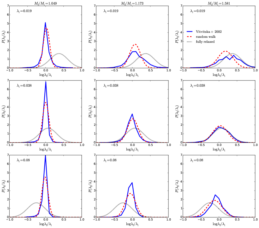
Figure 9: Comparison of the conditional halo spin distributions predicted by our random walk model with measurements from N-body simulations in Vitvitska et al. (2002). The nine panels correspond to those in Fig. 4 of Vitvitska et al. Each row corresponds to a range of the initial spin, $\lambda_{\rm i}$, with our estimated typical $\lambda_{\rm i}$ for that range given in the upper left corner of each panel. Each column corresponds to a range of the ratio, $M_{\rm f}/M_{\rm i}$, with $M_{\rm f}$ and $M_{\rm i}$ being the halo masses at adjacent snapshots, and our estimated typical $M_{\rm f}/M_{\rm i}$ being shown at the top of the column. In each panel, the blue solid line is the conditional spin distribution from Vitvitska et al., the red dashed line is the distribution calculated from equation (63) based on our random walk model, and the black dotted line shows the fully relaxed distribution expected in the random walk model for reference.

Using these estimated typical values, the corresponding conditional distributions can be calculated for the random walk model. Fig. 9 shows the comparison between the predictions of our simple random walk model and the results measured by Vitvitska et al. from their N-body simulations. The agreement is acceptable for a simple comparison.

Appendix D Simple AGN feedback model in GALFORM

The AGN feedback model used in the ‘Lacey16’ model was first introduced in Bower et al. (2006). Specifically, it assumes that the AGN feedback is in the radio mode (Croton et al., 2006), in which a relativistic jet generated by supermassive black hole (SMBH) accretion heats the halo gas and thus suppresses cooling.

In galform there are two conditions for effective AGN feedback. Firstly, the halo gas should be close to the slow cooling regime, in which the cooling is slower than the gravitational infall and a quasi-hydrostatic hot gaseous halo exists. This is motivated by the idea that only the gas close to this regime can maintain its pressure and thus the jet can interact and heat the halo gas effectively. This condition is tested by comparing the cooling time scale, $t_{\rm cool}$, and the free-fall time scale, $t_{\rm ff}$, at the cooling radius, $r_{\rm cool}$. Specifically, AGN feedback is assumed to be effective only if

$$t_{\rm cool}(r_{\rm cool})/t_{\rm ff}(r_{\rm cool})>1/\alpha_{\rm cool},$$ (64)

with $\alpha_{\rm cool}\sim 1$ an adjustable parameter. Consider that at earlier times the ratio $t_{\rm cool}(r_{\rm cool})/t_{\rm ff}(r_{\rm cool})$ is typically smaller, then increasing $\alpha_{\rm cool}$ causes AGN feedback to turn on earlier and thus enhances the suppression due to this feedback.

Secondly, the SMBH accretion rate should be significantly lower than the Eddington limit so that jets can be efficiently produced (Fanidakis et al., 2011), and the jet should be energetic enough to balance the cooling radiation. This motivates the following condition

$$f_{\rm Edd}L_{\rm Edd}(M_{\rm BH})>L_{\rm cool},$$ (65)

where $f_{\rm Edd}\ll 1$ is a parameter, $L_{\rm Edd}(M_{\rm BH})$ is the Eddington luminosity of a black hole with mass $M_{\rm BH}$, and $L_{\rm cool}$ is the cooling luminosity of the hot gas halo. In the ‘Lacey16’ model, $f_{\rm Edd}=0.01$.

Once the above two conditions are satisfied, the AGN feedback is assumed to be effective. In the GFC1 model, the increase of $r_{\rm cool}$ due to cooling is then set to zero, and then the associated mass and angular momentum cooling rates become zero.

In the new cooling model, since a different procedure is used to calculate $t_{\rm cool,avail}$, some modifications are needed. Specifically, when AGN feedback turns on, the energy previously radiated away, $E_{\rm cool}$, is set to zero because the halo gas is heated up. This causes $t_{\rm cool,avail}$ to reduce to zero. With this, $r_{\rm cool}$ does not increase and the halo cold gas component stops growing immediately. If this component has nonzero mass, then it can still deliver cold gas to the central galaxy. When a halo is close to the slow cooling regime, the halo cold gas component typically is very small, so the cold gas accretion onto the central galaxy should stop shortly after AGN feedback turns on.

References

- Baugh (2006) Baugh C. M., 2006, Reports on Progress in Physics, 69, 3101
- Baugh et al. (2005) Baugh C. M., Lacey C. G., Frenk C. S., Granato G. L., Silva L., Bressan A., Benson A. J., Cole S., 2005, MNRAS, 356, 1191
- Benson & Bower (2010) Benson A. J., Bower R., 2010, MNRAS, 405, 1573
- Benson & Bower (2011) Benson A. J., Bower R., 2011, MNRAS, 410, 2653
- Bertschinger (1989) Bertschinger E., 1989, ApJ, 340, 666
- Bett et al. (2007) Bett P., Eke V., Frenk C. S., Jenkins A., Helly J., Navarro J., 2007, MNRAS, 376, 215
- Binney (1977) Binney J., 1977, ApJ, 215, 483
- Birnboim & Dekel (2003) Birnboim Y., Dekel A., 2003, MNRAS, 345, 349
- Bower et al. (2006) Bower R. G., Benson A. J., Malbon R., Helly J. C., Frenk C. S., Baugh C. M., Cole S., Lacey C. G., 2006, MNRAS, 370, 645
- Cole & Lacey (1996) Cole S., Lacey C., 1996, MNRAS, 281, 716
- Cole et al. (2000) Cole S., Lacey C. G., Baugh C. M., Frenk C. S., 2000, MNRAS, 319, 168
- Croton et al. (2006) Croton D. J. et al., 2006, MNRAS, 365, 11
- Croton et al. (2016) Croton D. J. et al., 2016, ApJS, 222, 22
- De Lucia & Blaizot (2007) De Lucia G., Blaizot J., 2007, MNRAS, 375, 2
- De Lucia et al. (2010) De Lucia G., Boylan-Kolchin M., Benson A. J., Fontanot F., Monaco P., 2010, MNRAS, 406, 1533
- Driver et al. (2012) Driver S. P. et al., 2012, MNRAS, 427, 3244
- Eke et al. (1996) Eke V. R., Cole S., Frenk C. S., 1996, MNRAS, 282, 263
- Fanidakis et al. (2011) Fanidakis N., Baugh C. M., Benson A. J., Bower R. G., Cole S., Done C., Frenk C. S., 2011, MNRAS, 410, 53
- Font et al. (2008) Font A. S. et al., 2008, MNRAS, 389, 1619
- Garcia-Palacios (2007) Garcia-Palacios J. L., 2007, eprint arXiv:cond-mat/0701242
- Gardner (2001) Gardner J. P., 2001, ApJ, 557, 616
- Gonzalez-Perez et al. (2014) Gonzalez-Perez V., Lacey C. G., Baugh C. M., Lagos C. D. P., Helly J., Campbell D. J. R., Mitchell P. D., 2014, MNRAS, 439, 264
- Guo et al. (2011) Guo Q. et al., 2011, MNRAS, 413, 101
- Henriques et al. (2015) Henriques B. M. B., White S. D. M., Thomas P. A., Angulo R., Guo Q., Lemson G., Springel V., Overzier R., 2015, MNRAS, 451, 2663
- Jiang et al. (2008) Jiang C. Y., Jing Y. P., Faltenbacher A., Lin W. P., Li C., 2008, ApJ, 675, 1095
- Kauffmann et al. (1993) Kauffmann G., White S. D. M., Guiderdoni B., 1993, MNRAS, 264, 201
- Kereš et al. (2009) Kereš D., Katz N., Fardal M., Davé R., Weinberg D. H., 2009, MNRAS, 395, 160
- Kereš et al. (2005) Kereš D., Katz N., Weinberg D. H., Davé R., 2005, MNRAS, 363, 2
- Lacey & Cole (1993) Lacey C., Cole S., 1993, MNRAS, 262, 627
- Lacey et al. (2016) Lacey C. G. et al., 2016, MNRAS, 462, 3854
- Maller et al. (2002) Maller A. H., Dekel A., Somerville R., 2002, MNRAS, 329, 423
- Monaco et al. (2014) Monaco P., Benson A. J., De Lucia G., Fontanot F., Borgani S., Boylan-Kolchin M., 2014, MNRAS, 441, 2058
- Monaco et al. (2007) Monaco P., Fontanot F., Taffoni G., 2007, MNRAS, 375, 1189
- Moster et al. (2013) Moster B. P., Naab T., White S. D. M., 2013, MNRAS, 428, 3121
- Navarro et al. (1997) Navarro J. F., Frenk C. S., White S. D. M., 1997, ApJ, 490, 493
- Nelson et al. (2016) Nelson D., Genel S., Pillepich A., Vogelsberger M., Springel V., Hernquist L., 2016, MNRAS, 460, 2881
- Neto et al. (2007) Neto A. F. et al., 2007, MNRAS, 381, 1450
- Norberg et al. (2002) Norberg P. et al., 2002, MNRAS, 336, 907
- Parkinson et al. (2008) Parkinson H., Cole S., Helly J., 2008, MNRAS, 383, 557
- Rees & Ostriker (1977) Rees M. J., Ostriker J. P., 1977, MNRAS, 179, 541
- Shen et al. (2003) Shen S., Mo H. J., White S. D. M., Blanton M. R., Kauffmann G., Voges W., Brinkmann J., Csabai I., 2003, MNRAS, 343, 978
- Silk (1977) Silk J., 1977, ApJ, 211, 638
- Somerville et al. (2008) Somerville R. S., Hopkins P. F., Cox T. J., Robertson B. E., Hernquist L., 2008, MNRAS, 391, 481
- Springel et al. (2001) Springel V., White S. D. M., Tormen G., Kauffmann G., 2001, MNRAS, 328, 726
- Stevens et al. (2017) Stevens A. R. H., Lagos C. d. P., Contreras S., Croton D. J., Padilla N. D., Schaller M., Schaye J., Theuns T., 2017, MNRAS, 467, 2066
- Sutherland & Dopita (1993) Sutherland R. S., Dopita M. A., 1993, ApJS, 88, 253
- Viola et al. (2008) Viola M., Monaco P., Borgani S., Murante G., Tornatore L., 2008, MNRAS, 383, 777
- Vitvitska et al. (2002) Vitvitska M., Klypin A. A., Kravtsov A. V., Wechsler R. H., Primack J. R., Bullock J. S., 2002, ApJ, 581, 799
- Warren et al. (1992) Warren M. S., Quinn P. J., Salmon J. K., Zurek W. H., 1992, ApJ, 399, 405
- White & Frenk (1991) White S. D. M., Frenk C. S., 1991, ApJ, 379, 52
- White & Rees (1978) White S. D. M., Rees M. J., 1978, MNRAS, 183, 341
- Yoshida et al. (2002) Yoshida N., Stoehr F., Springel V., White S. D. M., 2002, MNRAS, 335, 762