Enabling Massive Deep Neural Networks
with the GraphBLAS

Abstract

Deep Neural Networks (DNNs) have emerged as a core tool for machine learning. The computations performed during DNN training and inference are dominated by operations on the weight matrices describing the DNN. As DNNs incorporate more stages and more nodes per stage, these weight matrices may be required to be sparse because of memory limitations. The GraphBLAS.org math library standard was developed to provide high performance manipulation of sparse weight matrices and input/output vectors. For sufficiently sparse matrices, a sparse matrix library requires significantly less memory than the corresponding dense matrix implementation. This paper provides a brief description of the mathematics underlying the GraphBLAS. In addition, the equations of a typical DNN are rewritten in a form designed to use the GraphBLAS. An implementation of the DNN is given using a preliminary GraphBLAS C library. The performance of the GraphBLAS implementation is measured relative to a standard dense linear algebra library implementation. For various sizes of DNN weight matrices, it is shown that the GraphBLAS sparse implementation outperforms a BLAS dense implementation as the weight matrix becomes sparser.

I Introduction

Machine learning describes the broad area of analysis and classification of data to create models for making predictions. Machine learning has been the foundation of artificial intelligence since its inception [1, 2, 3, 4, 5, 6, 7, 8]. Early machine learning applications included speech recognition [3], computer vision [4], and even board games [5, 9].

Figure 1: Typical network elements $i$ and $j$ showing connection weights $w$ (reproduced from [2])

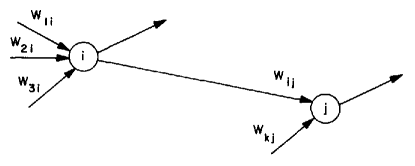
Using biological neuron inspired networks to implement machine learning was the topic of the first paper presented at the first machine learning conference in 1955 [1, 2] (see Figure 1). At this time, it was recognized that direct computational training of neural networks was computationally unfeasible [7]. The subsequent many-fold improvement in neural network computation and theory has made it possible to train neural networks that are capable of better-than-human performance in a variety of important artificial intelligence problems [10, 11, 12, 13]. Specifically, the availability of large corpora of validated data sets [14, 15, 16] and the increases in computation spurred by games [17, 18, 19, 20], have allowed the effective training of large deep neural networks (DNNs) with 100,000s of input features, $N$, and hundreds of layers, $L$, that are capable of choosing from among 100,000s categories, $M$ (see Figure 2).

Figure 2: Four layer ($L=4$) deep neural network architecture for categorizing images. The input features ${\bf y}_{0}$ of an image are passed through a series of network layers ${\bf W}_{k=0,1,2,3}$, with bias terms ${\bf b}_{k=0,1,2,3}$, that produce scores for categories ${\bf y}_{L=4}$. (Figure adapted from [21])

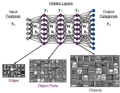
The impressive performance of large DNNs encourages the training and testing of even larger networks. However, increasing $N$, $L$, $M$ each by a factor 10 results in a 1000 fold increase in the memory required for a DNN. Because of these memory constraints, trade-offs are currently being made in terms of precision and accuracy to save storage and computation [22, 23]. Thus, there is significant interest in exploring the effectiveness of sparse DNN representations where many of the weight values are zero. As a comparison, the human brain has approximately 86 billion neurons and 150 trillion synapses [24]. Its graph representation would have approximately 2,000 edges per node, or a sparsity of $2\times 10^{3}/86\times 10^{9}=0.000002\%$.

If a large fraction of the DNN weights can be set to zero, storage and computation costs can be reduced proportionately. [25, 26]. The interest in sparse DNNs is not limited to their computational advantages. There has also been extensive theoretical work exploring the potential neuromorphic and algorithmic benefits of sparsity [27, 28, 29, 30]. Experts in DNN believe that sparsification of weight matrices will lead to better results.

As reported in the literature [31], sparsification of the weight matrices is achieved by first training the neural network with a full matrix, then removing those weights that are small, and finally retraining the pruned network. The resulting sparse weight matrix can be used during inference computation with the neural network. Therefore, sparse matrix solutions can be used both during the final stages of training as well as during inference.

Computation over sparse data structures has been a mainstay of the graph analysis community for many years. Graphs are among the most important abstract data structures in computer science, and the algorithms that operate on them are critical to applications in bioinformatics, computer networks, and social media [32, 33, 34, 35, 36]. Graphs have been shown to be powerful tools for modeling complex problems because of their simplicity and generality [37, 38]. For this reason, the field of graph algorithms has become one of the pillars of theoretical computer science, performing research in such diverse areas as combinatorial optimization, complexity theory, and topology. Graph algorithms have been adapted and implemented by the military, commercial industry, and researchers in academia, and have become essential in controlling the power grid, telephone systems, and, of course, computer networks.

The connection between graphs and DNNs lies in the standard matrix representation of graphs. The duality between the canonical representation of graphs as abstract collections of vertices and edges and a matrix representation has been a part of graph theory since its inception [39, 40]. Matrix algebra has been recognized as a useful tool in graph theory for nearly as long (see [41] and references therein, in particular [42, 43, 44, 45, 46, 47, 48]). Likewise, graph-based approaches have also been very useful in matrix calculations [49, 50, 51]. The modern description of the duality between graph algorithms and matrix mathematics (or sparse linear algebra) has been extensively covered in the literature and is summarized in the cited text [52]. This text has further spawned the development of the GraphBLAS math library standard (GraphBLAS.org)[53] that has been developed in a series of proceedings [54, 55, 56, 57, 58, 59, 60, 61] and implementations [62, 63, 64, 65, 66, 67, 68].

In theory, the GraphBLAS may represent an ideal interface for enabling massive DNNs on both conventional and custom hardware [69, 70, 71]. Almost all computations during DNN inferencing, and a significant fraction during training, are encompassed in forward propagation of inferred features at each stage of the network. Intra-stage forward propagation consists of multiplication of a weight matrix with a batch of input/output vectors, basically a multiplication of two matrices, followed by an element wise application of a non-linear function to the resulting matrix. In this paper we show that for sparse weight matrices these computations are performed much more efficiently by GraphBLAS implementations than by BLAS implementations.

The rest of this paper explores this proposition as follows. First, a brief description of the mathematics underlying the GraphBLAS is provided. Second, the mathematics of a common DNN are presented in a form designed to utilize the GraphBLAS. Third, an implementation of the DNN is given using a preliminary GraphBLAS C library. Fourth, the performance of the GraphBLAS implementation is measured relative to standard linear algebra library implementation. Finally, this paper concludes with a summary and recommendations on future work.

II GraphBLAS Mathematics

This section summarizes the GraphBLAS matrix mathematics relevant to the GraphBLAS DNN implementation. For a more complete description of the mathematics in the GraphBLAS see [52, 72, 73]. The foundational mathematical construct of matrix-based graph analysis is the adjacency matrix. From this construct, a more general definition of a matrix can be constructed. How such a matrix can be manipulated depends on the types of values in the matrix and the operations allowed on those values. Furthermore, the mathematical properties of the matrix values determine the mathematical properties of the whole matrix. Perhaps the most important aspect of the GraphBLAS mathematics is that it allows graph operations to be treated as Linear Systems. By exploiting the properties of linear systems, a GraphBLAS library can optimally order and even eliminate steps in a computation.

II-A Adjacency Matrix

Given an adjacency matrix $\mathbf{A}$, if

$$\mathbf{A}(i,j)=1$$

then there exists an edge going from vertex $i$ to vertex $j$ (see Figure 3). Likewise, if

$$\mathbf{A}(i,j)=0$$

then there is no edge from $i$ to $j$. Adjacency matrices can have direction, which means that $\mathbf{A}(i,j)$ may not be the same as $\mathbf{A}(j,i)$. Adjacency matrices can also have edge weights. If

$$\mathbf{A}(i,j)=a\neq 0$$

then the edge going from $i$ to $j$ is said to have weight $a$. Adjacency matrices provide a simple way to represent the connections between vertices in a graph. Adjacency matrices are often square, and both the out-vertices (rows) and the in-vertices (columns) are the same set of vertices. Adjacency matrices can be rectangular, in which case the out-vertices (rows) and the in-vertices (columns) are different sets of vertices. Such graphs are often called bipartite graphs. In summary, adjacency matrices can represent a wide range of graphs, which include any graph with any set of the following properties: directed, weighted, and/or bipartite.

Figure 3: (left) Seven-vertex graph with 12 edges. Each vertex is labeled with an integer. (right) $7\times 7$ adjacency matrix $\mathbf{A}$ representation of the graph. $\mathbf{A}$ has 12 nonzero entries corresponding to the edges in the graph.

II-B Matrix Values

A typical matrix has $m$ rows and $n$ columns of real numbers. Such a matrix can be denoted as

$$\mathbf{A}:\mathbb{R}^{m\times n}$$

The row and and column indexes of the matrix $\mathbf{A}$ are

$$i\in I=\{1,\ldots,m\}$$

and

$$j\in J=\{1,\ldots,n\}$$

so that any particular value $\mathbf{A}$ can be denoted as $\mathbf{A}(i,j)$. The row and column indices of matrices are natural numbers $I,J:\mathbb{N}$. A matrix of integers is denoted $\mathbf{A}:\mathbb{Z}^{m\times n}$, and a matrix of natural numbers is denoted $\mathbf{A}:\mathbb{N}^{m\times n}$. Using the above concepts, a matrix is defined as the following two-dimensional (2D) mapping

$$\mathbf{A}:I\times J\rightarrow\mathbb{S}$$

where the indices $I,J:\mathbb{Z}$ are finite sets of integers with $m$ and $n$ elements, respectively, and

$$\mathbb{S}\in\{\mathbb{R},\mathbb{Z},\mathbb{N},\ldots\}$$

is a set of scalars. Without loss of generality, matrices can be denoted

$$\mathbf{A}:\mathbb{S}^{m\times n}$$

A vector is a matrix in which either $m=1$ or $n=1$. A column vector is denoted $\mathbf{v}:\mathbb{S}^{m\times 1}$ or simply $\mathbf{v}:\mathbb{S}^{m}$. A row vector can be denoted $\mathbf{v}:\mathbb{S}^{1\times n}$ or simply $\mathbf{v}:\mathbb{S}^{n}$. A scalar is a single element of a set $s\in\mathbb{S}$ and has no matrix dimensions.

II-C Scalar Operations

Matrix operations are built on top of scalar operations that can be used for combining and scaling graph edge weights. The primary scalar operations are standard arithmetic addition, such as

$$1+1=2$$

and arithmetic multiplication, such as

$$2\times 2=4$$

These scalar operations of addition and multiplication can be defined to be a wide variety of functions. To prevent confusion with standard arithmetic addition and arithmetic multiplication, $\oplus$ will be used to denote scalar addition and $\otimes$ will be used to denote scalar multiplication. In this notation, standard arithmetic addition and arithmetic multiplication of real numbers

$$a,b,c\in\mathbb{R}$$

where

$$\oplus\equiv+~{}~{}~{}~{}~{}\text{and}~{}~{}~{}~{}~{}\otimes\equiv\times$$

results in

$$c=a\oplus b~{}~{}~{}~{}~{}~{}~{}~{}~{}\Rightarrow~{}~{}~{}~{}~{}~{}~{}~{}~{}c=a+b$$

and

$$c=a\otimes b~{}~{}~{}~{}~{}~{}~{}~{}~{}\Rightarrow~{}~{}~{}~{}~{}~{}~{}~{}~{}c=a\times b$$

Generalizing $\oplus$ and $\otimes$ to a variety of operations enables a wide range of algorithms on scalars of all different types (not just real or complex numbers).

Certain $\oplus$ and $\otimes$ combinations over certain sets of scalars are particularly useful, and referred to as semirings, because they preserve essential mathematical properties, such as additive commutativity

$$a\oplus b=b\oplus a$$

additive associativity

$$(a\oplus b)\oplus c=a\oplus(b\oplus c)$$

multiplicative associativity

$$(a\otimes b)\otimes c=a\otimes(b\otimes c)$$

and the distributivity of multiplication over addition

$$a\otimes(b\oplus c)=(a\otimes b)\oplus(a\otimes c)$$

The properties of commutativity, associativity, and distributivity are extremely useful properties for building graph applications because they allow the builder to swap operations without changing the result. Example combinations of $\oplus$ and $\otimes$ that preserve scalar commutativity, associativity, and distributivity include (but are not limited to) standard arithmetic

$$\oplus\equiv+~{}~{}~{}~{}~{}~{}~{}~{}~{}\otimes\equiv\times~{}~{}~{}~{}~{}~{}~{}~{}~{}a,b,c\in\mathbb{R}$$

max-plus algebras

$$\oplus\equiv\max~{}~{}~{}~{}~{}~{}~{}~{}~{}\otimes\equiv+~{}~{}~{}~{}~{}~{}~{}~{}~{}a,b,c\in\{-\infty\cup\mathbb{R}\}$$

max-min algebras

$$\oplus\equiv\max~{}~{}~{}~{}~{}~{}~{}~{}~{}\otimes\equiv\min~{}~{}~{}~{}~{}~{}~{}~{}~{}a,b,c\in\{\text{-}\infty\cup\mathbb{R}_{\leq 0}\}$$

finite (Galois) fields such as GF(2)

$$\oplus\equiv{\rm xor}~{}~{}~{}~{}~{}~{}~{}~{}~{}\otimes\equiv{\rm and}~{}~{}~{}~{}~{}~{}~{}~{}~{}a,b,c\in\{0,1\}$$

and power set algebras

$$\oplus\equiv\cup~{}~{}~{}~{}~{}~{}~{}~{}~{}\otimes\equiv\cap~{}~{}~{}~{}~{}~{}~{}~{}~{}a,b,c\subset\mathcal{P}(\mathbb{Z})$$

II-D Matrix Properties

Associativity, distributivity, and commutativity are very powerful properties that enable the construction of composable graph algorithms (i.e., operations can be reordered with the knowledge that the answers will remain unchanged). Composability makes it easy to build a wide range of graph algorithms with just a few functions. Given matrices

$$\mathbf{A},\mathbf{B},\mathbf{C}\in\mathbb{S}^{m\times n}$$

let their elements be specified by

$$a=\mathbf{A}(i,j)~{}~{}~{}~{}~{}b=\mathbf{B}(i,j)~{}~{}~{}~{}~{}c=\mathbf{C}(i,j)$$

Commutativity, associativity, and distributivity of scalar operations translates into similar properties on matrix operations in the following manner.

Element-wise additive commutativity of matrices

$$a\oplus b=b\oplus a~{}~{}~{}~{}~{}\Rightarrow~{}~{}~{}~{}~{}\mathbf{A}\oplus\mathbf{B}=\mathbf{B}\oplus\mathbf{A}$$

where matrix element-wise addition is given by

$$\mathbf{C}(i,j)=\mathbf{A}(i,j)\oplus\mathbf{B}(i,j)$$

Element-wise multiplicative commutativity of matrices

$$a\otimes b=b\otimes a~{}~{}~{}~{}~{}\Rightarrow~{}~{}~{}~{}~{}\mathbf{A}\otimes\mathbf{B}=\mathbf{B}\otimes\mathbf{A}$$

where matrix element-wise (Hadamard) multiplication is given by

$$\mathbf{C}(i,j)=\mathbf{A}(i,j)\otimes\mathbf{B}(i,j)$$

Element-wise additive associativity of matrices
$~{}~{}~{}~{}~{}~{}~{}~{}~{}~{}~{}~{}~{}~{}~{}~{}~{}(a\oplus b)\oplus c=a\oplus(b\oplus c)$
$~{}~{}~{}~{}~{}\Rightarrow~{}~{}~{}~{}~{}(\mathbf{A}\oplus\mathbf{B})\oplus\mathbf{C}=\mathbf{A}\oplus(\mathbf{B}\oplus\mathbf{C})$
Element-wise multiplicative associativity of matrices
$~{}~{}~{}~{}~{}~{}~{}~{}~{}~{}~{}~{}~{}~{}~{}~{}~{}(a\otimes b)\otimes c=a\otimes(b\otimes c)$
$~{}~{}~{}~{}~{}\Rightarrow~{}~{}~{}~{}~{}(\mathbf{A}\otimes\mathbf{B})\otimes\mathbf{C}=\mathbf{A}\otimes(\mathbf{B}\otimes\mathbf{C})$
Element-wise distributivity of matrices
$~{}~{}~{}~{}~{}~{}~{}~{}~{}~{}~{}~{}~{}~{}~{}~{}~{}a\otimes(b\oplus c)=(a\otimes b)\oplus(a\otimes c)$
$~{}~{}~{}~{}~{}\Rightarrow~{}~{}~{}~{}~{}\mathbf{A}\otimes(\mathbf{B}\oplus\mathbf{C})=(\mathbf{A}\otimes\mathbf{B})\oplus(\mathbf{A}\otimes\mathbf{C})$
Matrix multiply distributivity
$~{}~{}~{}~{}~{}~{}~{}~{}~{}~{}~{}~{}~{}~{}~{}~{}~{}a\otimes(b\oplus c)=(a\otimes b)\oplus(a\otimes c)$
$~{}~{}~{}~{}~{}\Rightarrow~{}~{}~{}~{}~{}~{}~{}~{}\mathbf{A}(\mathbf{B}\oplus\mathbf{C})=(\mathbf{A}\mathbf{B})\oplus(\mathbf{A}\mathbf{C})$
where matrix multiply

$$\mathbf{C}=\mathbf{A}{\oplus}.{\otimes}\mathbf{B}=\mathbf{A}\mathbf{B}$$

is given by

$${\bf C}(i,j)=\bigoplus_{k=1}^{l}{\bf A}(i,k)\otimes{\bf B}(k,j)$$

for matrices with dimensions

$${\bf A}:\mathbb{S}^{m\times l}~{}~{}~{}~{}~{}{\bf B}:\mathbb{S}^{l\times m}~{}~{}~{}~{}~{}{\bf C}:\mathbb{S}^{m\times n}$$

Matrix multiply associativity of matrices
$~{}~{}~{}~{}~{}~{}~{}~{}~{}~{}~{}~{}~{}~{}~{}~{}~{}a\otimes(b\oplus c)=(a\otimes b)\oplus(a\otimes c)$
$~{}~{}~{}~{}~{}\Rightarrow~{}~{}~{}~{}~{}~{}~{}~{}~{}~{}~{}(\mathbf{A}\mathbf{B})\mathbf{C}=\mathbf{A}(\mathbf{B}\mathbf{C})$

II-E 0-Element: No Graph Edge

Sparse matrices play an important role in graphs. Many implementations of sparse matrices reduce storage by not storing the 0-valued elements in the matrix. In adjacency matrices, the 0 element is equivalent to no edge from the vertex that is represented by the row to the vertex that is represented by the column. In incidence matrices, the 0 element is equivalent to the edge represented by the row not including the vertex that is represented by the column. In most cases, the 0 element is standard arithmetic 0, but in other cases it can be a different value. Nonstandard 0 values can be helpful when combined with different $\oplus$ and $\otimes$ operations. For example, in different contexts 0 might be $+\infty$, -$\infty$, or $\emptyset$ (empty set). For any value of 0, if the 0 element has certain properties with respect to scalar $\oplus$ and $\otimes$, then the sparsity of matrix operations can be managed efficiently. These properties are the additive identity

$$a\oplus 0=a$$

and the multiplicative annihilator

$$a\otimes 0=0$$

Example combinations of $\oplus$ and $\otimes$ that exhibit the additive identity and multiplicative annihilator include standard arithmetic (${+}.{\times}$) on real numbers $\mathbb{R}$, max-plus algebra (${\max}.{+}$) on real numbers with a defined minimal element $\{\text{-}\infty\cup\mathbb{R}\}$, and min-max algebra (${\min}.{\max}$) using non-negative real numbers with a maximal element $\{\mathbb{R}_{\geq 0}\cup\infty\}$. The above examples are a small selection of the operators and sets that are useful for building graph algorithms. Many more are possible. The ability to change the scalar values and operators while preserving the overall behavior of the graph operations is one of the principal benefits of using matrices for graph algorithms.

III Deep Neural Network Mathematics

The primary mathematical operation performed by a DNN network is the inference, or forward propagation, step. Inference is executed repeatedly during training to determine both the weight matrices ${\bf W}_{k}$ and the bias vectors ${\bf b}_{k}$ of the DNN. The inference computation shown in Figure 2 is given by

$${\bf y}_{k+1}=h({\bf W}_{k}{\bf y}_{k}+{\bf b}_{k})$$

where $h()$ is a non-linear function applied to each element of the vector. A commonly used function is the rectified linear unit (ReLU) given by

$$h({\bf y})=\max({\bf y},0)$$

which sets values less that 0 to 0 and leaves other values unchanged. When training a DNN, it is common to compute multiple ${\bf y}_{k}$ vectors at once in a batch that can be denoted as the matrix ${\bf Y}_{k}$. In matrix form, the inference step becomes

$${\bf Y}_{k+1}=h({\bf W}_{k}{\bf Y}_{k}+{\bf B}_{k})$$

where ${\bf B}_{k}$ is a replication of ${\bf b}_{k}$ along columns.

If $h()$ were a linear function, then the above equation could be solved exactly and the computation could be greatly simplified. However, current evidence suggests that the non-linearity of $h()$ is required for a DNN to be effective. Interestingly, the inference computation can be rewritten as a linear function over two different semirings

$${\bf y}_{k+1}={\bf W}_{k}{\bf y}_{k}\otimes{\bf b}_{k}\oplus 0$$

or in matrix form

$${\bf Y}_{k+1}={\bf W}_{k}{\bf Y}_{k}\otimes{\bf B}_{k}\oplus 0$$

where the $\oplus=\max$ and $\otimes=+$. Thus, ${\bf W}_{k}{\bf y}_{k}$ and ${\bf W}_{k}{\bf Y}_{k}$ are computed over the standard arithmetic ${+}.{\times}$ semiring

$$S_{1}=(\mathbb{R},+,\times,0,1)$$

while the $\oplus$ and $\otimes$ operation are performed over the ${\max}.{+}$ semiring

$$S_{2}=(\{\text{-}\infty\cup\mathbb{R}\},\max,+,\text{-}\infty,0)$$

Thus, the ReLU DNN can be written as a linear system that oscillates over two semirings $S_{1}$ and $S_{2}$. $S_{1}$ is the most widely used of semirings and performs standard correlation between vectors. $S_{2}$ is also a commonly used semiring for selecting optimal paths in graphs. Thus, the inference step of a ReLU DNN can be viewed as combining correlations of inputs and to choose optimal paths through the neural network. Finally, and perhaps most importantly, the GraphBLAS is designed to support the above semiring calculations over sparse matrices.

IV Deep Neural Network Implementation

The GraphBLAS C implementation of the above deep neural networks is extremely concise, as shown in Figure 4. Function dnn (line 4) computes a forward propagation step in a ReLU DNN with $L$ layers. We assume that all layers have the same number of neurons, $m$, which is not a big loss of generality when the matrices can be sparse. The forward step is computed for a minibatch of size $n$. ${\bf W}$ is an array of $m\times m$ weight matrices, where ${\bf W}[k]$ is the weight matrix for layer $k$. Correspondingly, ${\bf B}$ is an array of $m\times n$-element bias vectors, where ${\bf B}[k]$ is the bias for layer $k$. Finally, ${\bf Y}$ is an array of $m\times n$ matrices, where ${\bf Y}[k]$ is the output from layer $k-1$ and the input for layer $k$. (${\bf Y}[0]$ is the input and ${\bf Y}[L]$ the output for the entire network.)

⬇

1#include <math.h>

2#include <GraphBLAS.h>

3

4GrB_Info dnn(GrB_Matrix *Y, GrB_Matrix *W, GrB_Matrix *B, GrB_Index L)

5/*

6 * L - Number of layers

7 * W[0:L-1] - Array of m x m weight matrices

8 * B[0:L-1] - Array of m x n bias matrices

9 * Y[0:L] - Array of m x n layer-input/output matrices

10 */

11{

12 GrB_Monoid FP32Add; // Monoid <float,+,0.0>

13 GrB_Monoid_new(&FP32Add,GrB_FP32,GrB_PLUS_FP32,0.0f);

14 GrB_Semiring FP32AddMul; // Semiring <float,+,*,0.0>

15 GrB_Semiring_new(&FP32AddMul,FP32Add,GrB_TIMES_FP32);

16

17 GrB_Monoid FP32Max; // Monoid <float,max,-inf>

18 GrB_Monoid_new(&FP32Max,GrB_FP32,GrB_MAX_FP32,-INFINITY);

19 GrB_Semiring FP32MaxPlus; // Semiring <float,max,+,-inf>

20 GrB_Semiring_new(&FP32MaxPlus,FP32Max,GrB_PLUS_FP32);

21

22 GrB_Index m, n;

23 GrB_Matrix_nrows(&m,Y[0]); GrB_Matrix_ncols(&n,Y[0]);

24 GrB_Matrix Zero; // Zero = 0.0

25 GrB_Matrix_new(&Zero,GrB_FP32,m,n);

26 GrB_assign(Zero,GrB_NULL,GrB_NULL,0.0,GrB_ALL,m,GrB_ALL,n,GrB_NULL);

27

28 for(int k=0; k<L; k++)

29 {

30 GrB_mxm(Y[k+1],GrB_NULL,GrB_NULL,FP32AddMul,W[k],Y[k],GrB_NULL); // Y[k+1] = W[k]*Y[k]

31 GrB_eWiseMult(Y[k+1],GrB_NULL,GrB_NULL,FP32MaxPlus,Y[k+1],B[k],GrB_NULL); // Y[k+1] = W[k]*Y[k] + B[k]

32 GrB_eWiseAdd (Y[k+1],GrB_NULL,GrB_NULL,FP32MaxPlus,Y[k+1],Zero,GrB_NULL); // Y[k+1] = max(W[k]*Y[k] + B[k],0)

33 }

34

35 GrB_free(&Zero);

36 GrB_free(&FP32Add); GrB_free(&FP32Max);

37 GrB_free(&FP32AddMul); GrB_free(&FP32MaxPlus);

38

39 return GrB_SUCCESS;

40}

Figure 4: GraphBLAS implementation of ReLU DNN using the C API.

Lines 12–15 and 17–20 define the two semirings that we use: the arithmetic semiring (FP32AddMul) and the max-plus semiring (FP32MaxPlus). (In GraphBLAS, semirings are built from monoids and binary operators.)

Lines 22–23 extract the parameters $m$ and $n$ from matrix ${\bf Y}[0]$, which are the same for all layers. Lines 24–26 create an $m\times n$ matrix of zeros that will be used in the computation of the ReLU function. Lines 35–37 free the GraphBLAS objects created inside this function.

The main computation loop is in lines 28–33. Each iteration computes the forward step in one layer $k$ of the network. The matrix-multiply in line 30 computes the product of the weight matrix ${\bf W}[k]$ by the input matrix ${\bf Y}[k]$. That result is added to the bias matrix ${\bf B}[k]$ in line 31. ($+$ is the multiplicative operation of semiring FPR32MaxPlus.) Finally, line 32 performs the ReLU operation by selecting the maximum between the previous result and the zero matrix. ($\max$ is the additive operation of semiring FP32MaxPlus.)

V Experimental Evaluation

In this section we compare the performance of GraphBLAS implementation of the forward propagation calculations in ReLU DNN with the OpenBLAS implementation. As expected, when the weight matrix is dense, OpenBLAS outperforms the GraphBLAS implementation. The converse is true for sparse weight matrices.

V-A Experimental Platform and Middleware

All our experiments are performed on a IBM Power S824L server configured with 24 POWER8 cores running at 3.325 GHz. Each core is capable of running from 1 (single-thread or ST) to 8 (SMT8) simultaneous threads of execution. The server is configured with 512 GiB of memory, accessible through a total of 16 memory channels. Total bandwidth from processing cores to memory is over 400 GB/s, with two-thirds of that for reading from memory and one-third for writing to memory.

The operating system installed is Ubuntu 16.04 distribution of Linux for PowerPC Little Endian. All code as compiled with Gnu 5.4 compilers (gcc/g++). The GraphBLAS API was implemented as a compatibility layer on top of IBM’s Graph Processing Interface (GPI) library [74]. When parallel processing was used in GraphBLAS, it was accomplished transparently through GPI, which in turns relies on OpenMP for multithreaded processing. GPI transparently uses various storage formats and strategies for dividing the work among multiple threads. In our specific case, the weight matrices were represented in compressed sparse row (CSR) format and they were distributed by rows. For dense linear algebra, we use OpenBLAS version 0.2.18.

V-B Experimental Matrices

All weight matrices ${\bf W}$ are $m\times m$ square matrices of single-precision (32-bit) floating-point numbers. All layer-input/output matrices ${\bf Y}$ are tall and skinny $m\times 64$ matrices that represent a mini-batch of size 64.

We vary the size ($m$) as well as the sparsity of the matrices. For convenience of presentation, we define the inverse sparsity of a matrix as the total number of elements in the matrix divided by the number of nonzero elements. In other words, the larger the inverse sparsity of a matrix, the more sparse it is (the larger the fraction of zeros). When performing the dense linear algebra version of the computation, zeros are represented explicitly. When using GraphBLAS, sparse matrix representations are used and only the nonzeros are stored.

For the weight matrices ${\bf W}$ we vary the inverse sparsity all the way from 1 (dense matrix) to 262144 (only $0.0004\%$ of elements are nonzero). Although it would be possible to treat the input/output matrices as sparse, in our work we only consider dense ${\bf Y}$ matrices.

Initially, dense weight matrices are generating by populating each entry with a random number chosen from a $U[-1,3)$ distribution. Sparse weight matrices are generated from these dense matrices by selecting the location of nonzero entries using independent Bernoulli distributions and taking the corresponding entry value (generated from the $U[-1,3)$ distribution). Layer input matrices are generated using a $U[0,1)$ distribution for the entry values.

V-C Performance Measurements

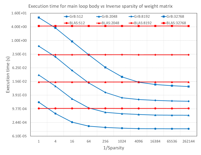
Figure 5 shows the single-threaded results for both GraphBLAS and dense linear algebra implementations of the ReLU DNN. We plot results for four different values of the matrix size parameter $n$ ($512$, $2048$, $8192$ and $32768$). For each matrix size, we show results for the two implementation versions (GrB - GraphBLAS, BLAS - dense linear algebra). The $x$-axis is the inverse sparsity of ${\bf W}$ and the $y$-axis is the average execution time of the main loop iteration in Figure 4. Both axes use a logarithmic scale.

Figure 5: Single-threaded (ST) results for GraphBLAS (GrB) and dense linear algebra (BLAS) implementations of the ReLU DNN. Results for GraphBLAS are in blue, whereas results for BLAS are in red. Each problem size uses a different marker. (Compare blue and red curves with the same marker.)

Figure 6: Multithreaded results for GraphBLAS (GrB) and dense linear algebra (BLAS) implementations of the ReLU DNN. Each plot is for one implementation (BLAS vs GraphBLAS) and a particular level of parallelism (4 vs 16 threads). Within each plot, speedup is shown as a function of inverse sparsity for four different problem sizes ($256$,$1024$,$4096$,$16384$).

As expected, and consistent through the various matrix sizes, the execution time of the dense linear algebra version is independent of the sparsity of ${\bf W}$. The GraphBLAS execution time goes down with the inverse sparsity of ${\bf W}$. For the measured problem sizes, GraphBLAS is $\sim 3$ times slower than BLAS for dense matrices. The performance advantage of BLAS starts to go down as we increase the inverse sparsity, until the two performances approximately match for inverse sparsity somewhat less than 4. For larger values of the inverse sparsity, GraphBLAS shows better performance.

When matrix ${\bf W}$ becomes very sparse (inverse sparsity $\gg n$), the execution time of GraphBLAS levels off, as it becomes dominated by the fixed cost of processing matrices in GraphBLAS. That is why the advantage of GraphBLAS over BLAS is higher for large, very sparse matrices For $n=32768$ and inverse sparsity $=4096$, GraphBLAS is $\sim 250$ times faster than the dense linear algebra implementation, or a $1000$-fold change in relative performances from the dense case.

Equally (or maybe more) important, is the advantage in memory consumption. A $32768\times 32768$ matrix for dense linear algebra has approximately 1 billion elements and consumes 4 GiB of storage (for single-precision data). The sparse matrix in GraphBLAS has storage that is essentially proportional to the number of nonzeros. That means that, depending on the inverse sparsity, GraphBLAS can accommodate problem sizes that are well beyond the means of current machines with the dense linear algebra approach.

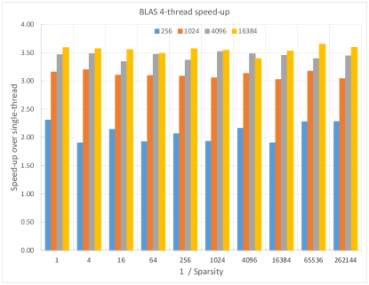
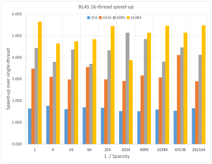
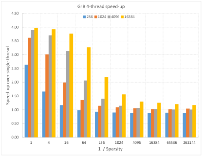
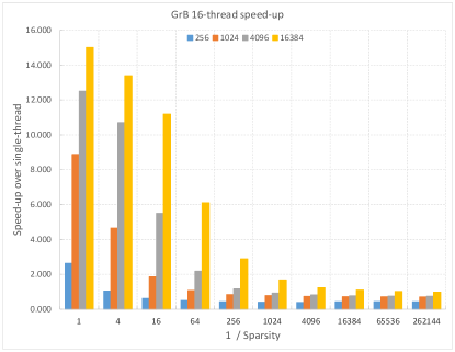
Figure 6 shows the speedup, as a function of inverse sparsity and for different sizes of the weight matrix, from multi-threaded execution with both 4 and 16 threads, for the BLAS and GraphBLAS implementations of the DNN code. The 4-thread measurements for GraphBLAS were taken with the four threads bound to four different cores on the same socket.

The 16-thread measurements for GraphBLAS were taken by assigning four threads to each of the four sockets, and binding the four threads assigned to a socket to four different cores. OpenBLAS does its own thread management.

As expected, the speedup behavior for BLAS varies little with the sparsity, and whatever variation we have is more likely due to measurement noise than anything intrinsic to the parallel execution. In general, speedup is better for larger matrices, since they better amortize any fixed overhead of parallelization.

The same behavior with respect to matrix size can be observed for the GraphBLAS implementation. The speedup for GraphBLAS, both with 4 and 16 threads, is very good for dense matrices, but shows a noticeable drop for all matrix sizes as the inverse sparsity increases. This is expected, since the total work that has to be executed in parallel goes down significantly as the inverse sparsity grows.

V-D Analysis of GraphBLAS Execution Times

The similarity in the shape of the curves for GraphBLAS performance in Figure 5 suggests that some common parameters or scaling laws define the shape of these curves. In Figure 7 we plot three such parameters and discuss their interpretation and significance. These are: 1) Ratio of BLAS/GraphBLAS execution times, 2) Slope of GraphBLAS execution time, and 3) Saturation value of the execution time. We also plot the scaling of BLAS performance normalized to matrix size. Since only relative performance is relevant to reasoning about scaling, all measures are also scaled to their value for $4096\times 4096$ weight matrix.

The time taken by BLAS for dense weight matrices of various sizes, normalized by the number of elements in the matrix is shown with legend BLAS. As mentioned in the preceding paragraph, it is further normalized by the time taken for a $4096\times 4096$ matrix. As expected, the execution time normalized to number of elements in the matrix is almost invariant. We believe that for matrices larger than $4096\times 4096$, normalized execution time increases because data is occasionally accessed from lower levels of cache hierarchy. For matrices smaller than $4096\times 4096$, normalized execution time is slightly higher because general overheads become non-negligible compared to the compute cycles devoted to the kernel calculations.

The curve with legend GraphBLAS/BLAS ratio is the ratio of run time for GraphBLAS implementation for $n\times n$ dense weight matrix scaled by the BLAS run time for the same weight matrix. This is an estimate of per element processing cost for BLAS and GraphBLAS implementations. For $4096\times 4096$ matrix it is 3.2 and is relatively invariant across weight matrix sizes. In Figure 5 it is the distance between the $y$-axis intercept of the GraphBLAS and BLAS performance curves for a given matrix size. One can readily observe that this ratio is inversely correlated to scaled BLAS performance.

Figure 7: The various parameters of execution time curves of Figure 5, normalized to their value at 4096*4096 matrix, plotted as a function of weight matrix size.

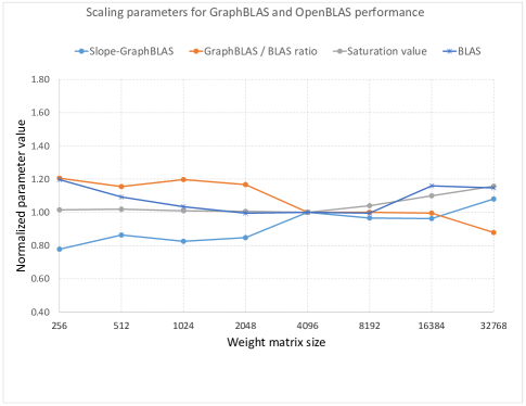The curve with legend Slope GraphBLAS is an estimate of the derivative of GraphBLAS execution time with respect to sparsity, evaluated at sparsity value of 1. It is computed as $(T_{S=1}-T_{S=1/4})/0.75\times n^{2}$, ratio of the difference between the execution times and the number of non-zero elements in the weight matrix for the two sparsity values. In this equation $S$ is the sparsity value. That is, the ratio of the number of non-zero entries to the total number of entries. This too is invariant across matrix sizes establishing that GraphBLAS performance for relative dense matrices is invariant to matrix size. This slope is the per element computing cost when the matrix has many non-zero elements per row. The values shown are normalized to the slope for $4096\times 4096$ weight matrix.

The curve with the legend Saturation value shows the execution time of GraphBLAS for weight matrices of sparsity $2^{-18}$, normalize by the size (number of rows, which equals the number of columns) of the matrix. For the $512\times 512$ matrix this sparsity amounts to one element in the whole matrix. For the $32768\times 32768$ matrix, it amounts to one element in every eight rows. This measure approximates the overhead of processing an almost empty matrix in GraphBLAS, and establishes it is proportional to the number of rows/columns of the matrix. The slightly higher values for larger matrix sizes are probably due to the large matrices having a larger fraction of non-empty rows. Once again, the values shown are normalized to the saturation value for a $4096\times 4096$ weight matrix.

VI Conclusions

Matrix operations involving weight matrices of DNNs represent the bulk of computation in the training and inferencing of DNNs. As the number of stages in the DNN and the number of nodes in each stage increase to handle more complex classification tasks, the weight matrices will become sparse. In this paper we have shown that the key DNN computations can be represented in GraphBLAS, a library interface defined for sparse matrix algebra. Furthermore, we have shown that the key step of forward propagation, with ReLU as the nonlinearity, can be performed much more efficiently with GraphBLAS implementation as compared to BLAS implementation when the weight matrices are sparse.

References

- [1] W. H. Ware, “Introduction to session on learning machines,” in Proceedings of the March 1-3, 1955, western joint computer conference. ACM, 1955, pp. 85–85.
- [2] W. A. Clark and B. G. Farley, “Generalization of pattern recognition in a self-organizing system,” in Proceedings of the March 1-3, 1955, western joint computer conference. ACM, 1955, pp. 86–91.
- [3] O. G. Selfridge, “Pattern recognition and modern computers,” in Proceedings of the March 1-3, 1955, western joint computer conference. ACM, 1955, pp. 91–93.
- [4] G. Dinneen, “Programming pattern recognition,” in Proceedings of the March 1-3, 1955, western joint computer conference. ACM, 1955, pp. 94–100.
- [5] A. Newell, “The chess machine: an example of dealing with a complex task by adaptation,” in Proceedings of the March 1-3, 1955, western joint computer conference. ACM, 1955, pp. 101–108.
- [6] J. McCarthy, M. L. Minsky, N. Rochester, and C. E. Shannon, “A proposal for the dartmouth summer research project on artificial intelligence, august 31, 1955,” AI magazine, vol. 27, no. 4, p. 12, 2006.
- [7] M. Minsky and O. G. Selfridge, “Learning in random nets,” in Information theory : papers read at a symposium on information theory held at the Royal Institution, London, August 29th to September 2nd. Butterworths, London, 1960, pp. 335–347.
- [8] M. Minsky, “Steps toward artificial intelligence,” Proceedings of the IRE, vol. 49, no. 1, pp. 8–30, 1961.
- [9] A. L. Samuel, “Some studies in machine learning using the game of checkers,” IBM Journal of research and development, vol. 3, no. 3, pp. 210–229, 1959.
- [10] R. Lippmann, “An introduction to computing with neural nets,” IEEE Assp magazine, vol. 4, no. 2, pp. 4–22, 1987.
- [11] D. A. Reynolds, T. F. Quatieri, and R. B. Dunn, “Speaker verification using adapted gaussian mixture models,” Digital signal processing, vol. 10, no. 1-3, pp. 19–41, 2000.
- [12] A. Krizhevsky, I. Sutskever, and G. E. Hinton, “Imagenet classification with deep convolutional neural networks,” in Advances in neural information processing systems, 2012, pp. 1097–1105.
- [13] Y. LeCun, Y. Bengio, and G. Hinton, “Deep learning,” Nature, vol. 521, no. 7553, pp. 436–444, 2015.
- [14] J. P. Campbell, “Testing with the yoho cd-rom voice verification corpus,” in Acoustics, Speech, and Signal Processing, 1995. ICASSP-95., 1995 International Conference on, vol. 1. IEEE, 1995, pp. 341–344.
- [15] Y. LeCun, C. Cortes, and C. J. Burges, “The mnist database of handwritten digits,” 1998.
- [16] J. Deng, W. Dong, R. Socher, L.-J. Li, K. Li, and L. Fei-Fei, “Imagenet: A large-scale hierarchical image database,” in Computer Vision and Pattern Recognition, 2009. CVPR 2009. IEEE Conference on. IEEE, 2009, pp. 248–255.
- [17] M. Campbell, A. J. Hoane, and F.-h. Hsu, “Deep blue,” Artificial intelligence, vol. 134, no. 1-2, pp. 57–83, 2002.
- [18] M. P. McGraw-Herdeg, D. P. Enright, and B. S. Michel, “Benchmarking the nvidia 8800gtx with the cuda development platform,” HPEC 2007 Proceedings, 2007.
- [19] A. Kerr, D. Campbell, and M. Richards, “Gpu performance assessment with the hpec challenge,” in HPEC Workshop 2008, 2008.
- [20] E. A. Epstein, M. I. Schor, B. Iyer, A. Lally, E. W. Brown, and J. Cwiklik, “Making watson fast,” IBM Journal of Research and Development, vol. 56, no. 3.4, pp. 15–1, 2012.
- [21] H. Lee, R. Grosse, R. Ranganath, and A. Y. Ng, “Convolutional deep belief networks for scalable unsupervised learning of hierarchical representations,” in Proceedings of the 26th annual international conference on machine learning. ACM, 2009, pp. 609–616.
- [22] A. Lavin and S. Gray, “Fast algorithms for convolutional neural networks,” in Proceedings of the IEEE Conference on Computer Vision and Pattern Recognition, 2016, pp. 4013–4021.
- [23] N. P. Jouppi, C. Young, N. Patil, D. Patterson, G. Agrawal, R. Bajwa, S. Bates, S. Bhatia, N. Boden, A. Borchers et al., “In-datacenter performance analysis of a tensor processing unit,” arXiv preprint arXiv:1704.04760, 2017.
- [24] F. A. Azevedo, L. R. Carvalho, L. T. Grinberg, J. M. Farfel, R. E. Ferretti, R. E. Leite, W. J. Filho, R. Lent, and S. Herculano-Houzel, “Equal numbers of neuronal and nonneuronal cells make the human brain an isometrically scaled-up primate brain,” The Journal of Comparative Neurology, vol. 513, no. 5, pp. 532–541, 2009. [Online]. Available: http://dx.doi.org/10.1002/cne.21974
- [25] S. Shi and X. Chu, “Speeding up convolutional neural networks by exploiting the sparsity of rectifier units,” arXiv preprint arXiv:1704.07724, 2017.
- [26] F. N. Iandola, S. Han, M. W. Moskewicz, K. Ashraf, W. J. Dally, and K. Keutzer, “Squeezenet: Alexnet-level accuracy with 50x fewer parameters and¡ 0.5 mb model size,” arXiv preprint arXiv:1602.07360, 2016.
- [27] H. Lee, C. Ekanadham, and A. Y. Ng, “Sparse deep belief net model for visual area v2,” in Advances in neural information processing systems, 2008, pp. 873–880.
- [28] Y.-l. Boureau, Y. L. Cun et al., “Sparse feature learning for deep belief networks,” in Advances in neural information processing systems, 2008, pp. 1185–1192.
- [29] X. Glorot, A. Bordes, and Y. Bengio, “Deep sparse rectifier neural networks.” in Aistats, vol. 15, no. 106, 2011, p. 275.
- [30] D. Yu, F. Seide, G. Li, and L. Deng, “Exploiting sparseness in deep neural networks for large vocabulary speech recognition,” in Acoustics, Speech and Signal Processing (ICASSP), 2012 IEEE International Conference on. IEEE, 2012, pp. 4409–4412.
- [31] S. Han, H. Mao, and W. J. Dally, “Deep compression: Compressing deep neural network with pruning, trained quantization and huffman coding,” CoRR, vol. abs/1510.00149, 2015. [Online]. Available: http://arxiv.org/abs/1510.00149
- [32] B. Hendrickson and T. G. Kolda, “Graph partitioning models for parallel computing,” Parallel computing, vol. 26, no. 12, pp. 1519–1534, 2000.
- [33] D. Ediger, K. Jiang, J. Riedy, and D. A. Bader, “Massive streaming data analytics: A case study with clustering coefficients,” in Parallel & Distributed Processing, Workshops and Phd Forum (IPDPSW), 2010 IEEE International Symposium on. IEEE, 2010, pp. 1–8.
- [34] D. Ediger, J. Riedy, D. A. Bader, and H. Meyerhenke, “Tracking structure of streaming social networks,” in Parallel and Distributed Processing Workshops and Phd Forum (IPDPSW), 2011 IEEE International Symposium on. IEEE, 2011, pp. 1691–1699.
- [35] J. Riedy, D. A. Bader, and H. Meyerhenke, “Scalable multi-threaded community detection in social networks,” in Parallel and Distributed Processing Symposium Workshops & PhD Forum (IPDPSW), 2012 IEEE 26th International. IEEE, 2012, pp. 1619–1628.
- [36] J. Riedy and D. A. Bader, “Multithreaded community monitoring for massive streaming graph data,” in Parallel and Distributed Processing Symposium Workshops & PhD Forum (IPDPSW), 2013 IEEE 27th International. IEEE, 2013, pp. 1646–1655.
- [37] E. Bergamini, H. Meyerhenke, and C. L. Staudt, “Approximating betweenness centrality in large evolving networks,” in 2015 Proceedings of the Seventeenth Workshop on Algorithm Engineering and Experiments (ALENEX). SIAM, 2015, pp. 133–146.
- [38] E. Bergamini and H. Meyerhenke, “Approximating betweenness centrality in fully dynamic networks,” Internet Mathematics, vol. 12, no. 5, pp. 281–314, 2016.
- [39] D. König, “Graphen und matrizen (graphs and matrices),” Mat. Fiz. Lapok, vol. 38, no. 1931, pp. 116–119, 1931.
- [40] ——, Theorie der endlichen und unendlichen Graphen: Kombinatorische Topologie der Streckenkomplexe. Akademische Verlagsgesellschaft mbh, 1936, vol. 16.
- [41] F. Harary, Graph Theory. Addison-Wesley, Reading, MA, 1969.
- [42] G. Sabidussi, “Graph multiplication,” Mathematische Zeitschrift, vol. 72, no. 1, pp. 446–457, 1959.
- [43] P. M. Weichsel, “The Kronecker product of graphs,” Proceedings of the American mathematical society, vol. 13, no. 1, pp. 47–52, 1962.
- [44] M. McAndrew, “On the product of directed graphs,” Proceedings of the American Mathematical Society, vol. 14, no. 4, pp. 600–606, 1963.
- [45] H. Teh and H. Yap, “Some construction problems of homogeneous graphs,” Bulletin of the Mathematical Society of Nanying University, vol. 1964, pp. 164–196, 1964.
- [46] A. Hoffman and M. McAndrew, “The polynomial of a directed graph,” Proceedings of the American Mathematical Society, vol. 16, no. 2, pp. 303–309, 1965.
- [47] F. Harary and C. A. Trauth, Jr, “Connectedness of products of two directed graphs,” SIAM Journal on Applied Mathematics, vol. 14, no. 2, pp. 250–254, 1966.
- [48] R. A. Brualdi, “Kronecker products of fully indecomposable matrices and of ultrastrong digraphs,” Journal of Combinatorial Theory, vol. 2, no. 2, pp. 135–139, 1967.
- [49] S. Parter, “The use of linear graphs in gauss elimination,” SIAM review, vol. 3, no. 2, pp. 119–130, 1961.
- [50] M. Fiedler, “Algebraic connectivity of graphs,” Czechoslovak mathematical journal, vol. 23, no. 2, pp. 298–305, 1973.
- [51] J. R. Gilbert, “Predicting structure in sparse matrix computations,” SIAM Journal on Matrix Analysis and Applications, vol. 15, no. 1, pp. 62–79, 1994.
- [52] J. Kepner and J. Gilbert, Graph Algorithms in the Language of Linear Algebra. SIAM, 2011.
- [53] T. Mattson, D. Bader, J. Berry, A. Buluc, J. Dongarra, C. Faloutsos, J. Feo, J. Gilbert, J. Gonzalez, B. Hendrickson et al., “Standards for graph algorithm primitives,” in High Performance Extreme Computing Conference (HPEC). IEEE, 2013, pp. 1–2.
- [54] J. Kepner, “GraphBLAS special session,” in High Performance Extreme Computing Conference (HPEC). IEEE, 2013.
- [55] T. Mattson, “Workshop on graph algorithms building blocks,” IPDPS, 2014.
- [56] ——, “GraphBLAS special session,” in High Performance Extreme Computing Conference (HPEC). IEEE, 2014.
- [57] ——, “Workshop on graph algorithms building blocks,” IPDPS, 2015.
- [58] A. Buluç, “GraphBLAS special session,” in High Performance Extreme Computing Conference (HPEC). IEEE, 2015.
- [59] T. Mattson, “Workshop on graph algorithms building blocks,” IPDPS, 2016.
- [60] A. Buluç and S. McMillan, “GraphBLAS special session,” in High Performance Extreme Computing Conference (HPEC). IEEE, 2016.
- [61] A. Buluç and T. Mattson, “Workshop on graph algorithms building blocks,” IPDPS, 2017.
- [62] A. Buluç and J. R. Gilbert, “The combinatorial blas: Design, implementation, and applications,” The International Journal of High Performance Computing Applications, vol. 25, no. 4, pp. 496–509, 2011.
- [63] J. Kepner, W. Arcand, W. Bergeron, N. Bliss, R. Bond, C. Byun, G. Condon, K. Gregson, M. Hubbell, J. Kurz, A. McCabe, P. Michaleas, A. Prout, A. Reuther, A. Rosa, and C. Yee, “Dynamic distributed dimensional data model (D4M) database and computation system,” in Acoustics, Speech and Signal Processing (ICASSP), 2012 IEEE International Conference on. IEEE, 2012, pp. 5349–5352.
- [64] K. Ekanadham, B. Horn, J. Jann, M. Kumar, J. Moreira, P. Pattnaik, M. Serrano, G. Tanase, and H. Yu, “Graph programming interface: Rationale and specification,” IBM Research Report, RC25508 (WAT1411-052) November 19, Tech. Rep., 2014.
- [65] D. Hutchison, J. Kepner, V. Gadepally, and A. Fuchs, “Graphulo implementation of server-side sparse matrix multiply in the Accumulo database,” in High Performance Extreme Computing Conference (HPEC). IEEE, 2015, pp. 1–7.
- [66] M. J. Anderson, N. Sundaram, N. Satish, M. M. A. Patwary, T. L. Willke, and P. Dubey, “Graphpad: Optimized graph primitives for parallel and distributed platforms,” in Parallel and Distributed Processing Symposium, 2016 IEEE International. IEEE, 2016, pp. 313–322.
- [67] Y. Wang, A. Davidson, Y. Pan, Y. Wu, A. Riffel, and J. D. Owens, “Gunrock: A high-performance graph processing library on the gpu,” in Proceedings of the 21st ACM SIGPLAN Symposium on Principles and Practice of Parallel Programming. ACM, 2016, p. 11.
- [68] P. Zhang, M. Zalewski, A. Lumsdaine, S. Misurda, and S. McMillan, “Gbtl-cuda: Graph algorithms and primitives for gpus,” IPDPS Graph Algorithms Building Blocks, pp. 912–920, 2016.
- [69] W. S. Song, J. Kepner, H. T. Nguyen, J. I. Kramer, V. Gleyzer, J. R. Mann, A. H. Horst, L. L. Retherford, R. A. Bond, N. T. Bliss et al., “3-d graph processor,” in Workshop on High Performance Embedded Workshop (HPEC). MIT Lincoln Laboratory, 2010.
- [70] W. S. Song, J. Kepner, V. Gleyzer, H. T. Nguyen, and J. I. Kramer, “Novel graph processor architecture,” Lincoln Laboratory Journal, vol. 20, no. 1, pp. 92–104, 2013.
- [71] W. S. Song, V. Gleyzer, A. Lomakin, and J. Kepner, “Novel graph processor architecture, prototype system, and results,” in High Performance Extreme Computing Conference (HPEC). IEEE, 2016, pp. 1–7.
- [72] J. Kepner, P. Aaltonen, D. Bader, A. Buluç, F. Franchetti, J. Gilbert, D. Hutchison, M. Kumar, A. Lumsdaine, H. Meyerhenke, S. McMillan, J. Moreira, J. Owens, C. Yang, M. Zalewski, and T. Mattson, “Mathematical foundations of the GraphBLAS,” in High Performance Extreme Computing Conference (HPEC). IEEE, 2016, pp. 1–9.
- [73] J. Kepner and H. Jananthan, Mathematics of big data: Spreadsheets, databases, matrices, and graphs. MIT Press, 2017.
- [74] W. Horn, M. Kumar, J. Jann, J. Moreira, P. Pattnaik, M. Serrano, G. Tanase, and H. Yu, “Graph Programming Interface (GPI): A linear algebra programming model for large scale graph computations,” International Journal of Parallel Programming, pp. 1–29, 2017. [Online]. Available: http://dx.doi.org/10.1007/s10766-016-0481-y