An evaluation of large-scale methods
for image instance and class discovery

Abstract

This paper aims at discovering meaningful subsets of related images from large image collections without annotations. We search groups of images related at different levels of semantic, i.e., either instances or visual classes. While k-means is usually considered as the gold standard for this task, we evaluate and show the interest of diffusion methods that have been neglected by the state of the art, such as the Markov Clustering algorithm.

We report results on the ImageNet and the Paris500k instance dataset, both enlarged with images from YFCC100M. We evaluate our methods with a labelling cost that reflects how much effort a human would require to correct the generated clusters.

Our analysis highlights several properties. First, when powered with an efficient GPU implementation, the cost of the discovery process is small compared to computing the image descriptors, even for collections as large as 100 million images. Second, we show that descriptions selected for instance search improve the discovery of object classes. Third, the Markov Clustering technique consistently outperforms other methods; to our knowledge it has never been considered in this large scale scenario.

1 Introduction

Large collections of images are now prominent. The diversity of their visual content is high, and due to the “long-tail” issue well known by researchers working on text data, a few classes are very frequent, but the vast majority of the classes do not occur often. In the visual world we consider, it is hard to collect enough labelled data for most of the visual entities. This is in contrast with the balanced and strongly supervised setting of ImageNet Dong et al. (2009).

In our paper, we consider the problem of visual discovery. The task is to automatically suggest subsets of related images, without employing any label or tag. This differs from semi-supervised learning Fergus et al. (2009), where a fraction of the dataset is annotated beforehand with a pre-defined set of labels. It is also different from noisy supervision with unreliable hashtags, as in Joulin et al. Joulin et al. (2016). Most of the early work on discovery focused on instances Chum and Matas (2010), location recognition or city-level 3D reconstruction Agarwal et al. (2009); Frahm et al. (2010), where the best methods are powered by spatial recognition, guaranteeing high matching performance by drastically reducing the rate of false positives. Such methods are not applicable to non-rigid instances or classes. Few studies have considered the problem of class discovery, which is harder to define from a user interest point of view, beyond classical clustering metrics like the square loss.

We address a general discovery scenario, with an application in mind where we need to detect visually related images from a novel collection for the purpose of navigation, trend analysis or fast labelling. In this context, the user interest could be related to categories depicted in the collection but unseen at train time, or to specific objects such as paintings or locations. For example, given a collection of landmark images, how can we determine that the user’s interest is in distinguishing between Romanesque and Gothic architectures, or between the façade of the Notre Dame cathedral and other buildings? This problem is challenging because it addresses different levels of semantics, which are not necessarily well identified by a single kind of descriptor. For this purpose, we study recent candidate methods initially designed for instance recognition and image classification, namely R-MAC Tolias et al. (2016) and Resnet He et al. (2016), and several discovery mechanisms based on kNN graphs and clustering. Our approach exploits dataset characteristics: if the dataset contains many Notre Dame images, then they will get a group of their own, otherwise they can be grouped with other Gothic cathedrals.

Our paper makes the following main contributions:

• We propose an evaluation protocol for the proposed discovery task, which accounts for different semantic levels and is extensible to arbitrarily large datasets using a distractor dataset.

• We evaluate the performance and scalability of four clustering strategies, namely k-means, agglomerative clustering, power-iterative clustering and an improved variant of the Markov Cluster Algorithm.

• We show that when efficient CPU and GPU implementations of kNN search are used, diffusion methods can easily handle 10- to 100- million scale datasets, i.e., one or two orders of magnitude larger than the most accurate competing methods based on approximate k-means or diffusion, e.g., the works of Avrithis et al. Avrithis et al. (2015) and Iscen et al. Iscen et al. (2017b, a).

• We apply Markov Clustering to this task, and show it significantly outperforms k-means, which is considered as a top-line in other approaches.

As a result of our study, we provide recommendations for the discovery task, and propose choices that will hopefully serve as baselines in future work on large-scale discovery.

The rest of this paper is organized as follows. After introducing related work in Section 2, we introduce the large-scale discovery strategy in Section 3. The experiments and evaluation are presented in Section 4. Section 5 concludes the paper.

2 Related work

This section presents related work on visual discovery, associated with various problems like image description, classification and efficient clustering. Note that typical descriptors employed for class and instance recognition are different. Even though these problems mainly differ by composition granularity, they are addressed by two distinct tasks and evaluation protocols in the literature, namely image classification and instance search/image search. We provide background references on these related tasks and cite relevant description schemes that we employ as input for our method. We also discuss prior art on discovery, including algorithms that aim to improve scalability.

Image descriptors for class and instance discovery.

Traditionally, discovery Gong et al. (2014); Babenko et al. (2014); Tolias et al. (2016) uses image description methods borrowed from image matching, in particular those based on keypoint indexing Lowe (2004); Sivic and Zisserman (2003); Philbin et al. (2008); Tolias et al. (2013), with impressive results when fine-tuned for rigid objects, like buildings on the Oxford dataset Gordo et al. (2016); Radenović et al. (2016). For class discovery or semi-supervised labelling Fergus et al. (2009), semantic global descriptors like GIST Oliva and Torralba (2001) are preferred. Recently, classification performance has substantially improved with deep CNN architectures Simonyan and Zisserman (2014); He et al. (2016) which are therefore compelling choices for our purpose.

Weiler & Fergus Zeiler and Fergus (2014) visualize the object classes corresponding to different activation levels of AlexNet and show that semantic levels correspond to layers. For networks trained on a dataset with general visual classes like ImageNet, this hints at employing different layers of the network to enable discovery at different levels of semantic. Interestingly, the winning entry of ImageNet 2015, the so-called ResNet He et al. (2016), substantially improves accuracy by introducing skip connections in CNN architectures. However, for similar instance search, aggregation strategies Babenko and Lempitsky (2015) significantly outperform the choice Babenko et al. (2014) of simply extracting the activation at a given layer.

Works on co-segmentation Joulin et al. (2012) and the approach of Cho et al.. Cho et al. (2015) aim at discovering objects by matching image regions. These techniques are accurate but do not scale beyond a few thousand images as they require maintaining and processing local descriptors. In contrast, we use only global image descriptors.

Clustering & kNN Graph.

The gold-standard clustering method is k-means. Min-hashing Zhao et al. (2013) or binary k-means Gong et al. (2015) have also been considered for visual discovery. However algorithms that can take an arbitrary metric on input are more flexible. We consider in particular clustering methods based on a diffusion process, which share some connections with spectral clustering Boaz Nadler and Kevrekidis (2008). They are an efficient way of clustering images given a matrix of input similarity, or a kNN graph, and have been successfully used in a semi-supervised discovery setup Fergus et al. (2009). In Philbin and Zisserman (2008), a kNN graph is clustered with spectral clustering, which amounts to computing the $k$ eigenvectors associated with the $k$ largest eigenvalues of the graph, and clustering these eigenvectors. Interestingly, when the eigenvalues are obtained via Lanczos iterations (Golub and Loan, 2013, Chapter 10), the basic operation is still a kind of diffusion process.

This is also related to Power Iteration Clustering Lin and Cohen (2010). In our experiments we evaluate a simplified version of it proposed by Cho et al. Cho and Lee (2012) to find clusters: instead of clustering a low-dim space, we follow the path to the mode of each cluster. We refer the reader to Donoser and Bischof (2013) for a review of diffusion processes and matrix normalizations. Approximate algorithms Dong et al. (2011); Kalantidis et al. (2016); Avrithis et al. (2015); Harwood and Drummond (2016) have been proposed to efficiently produce the kNN graph used as input of iterative/diffusion methods, some of them operating in the compressed domain.

Similarity or distance normalization.

In retrieval applications, images are typically ordered by distances, meaning that only the relative distances to the query matter. However, discovery is a detection problem, and its quality depends on the absolute distances between all pairs of descriptors. When building a kNN graph, it is therefore important to ensure that edges originating from different nodes have comparable weights. This problem is well known in spectral clustering Zelnik-Manor and Perona (2004) and computer vision Perronnin et al. (2009); Scheirer et al. (2012), and has led authors to propose different normalization pre-processing of distances or similarities. For instance, the contextual dissimilarity measure Jégou et al. (2007) regularizes distances by local updates. Another related work by Omercevic et al. Omercevic et al. (2007) uses the distribution of points relatively far away from the current point to regularize the distance distribution. This empirical choice is supported Furon and Jégou (2013) by extreme value theory and estimation, which was also been successful to calibrate the output of classifiers Scheirer et al. (2012). We use a simpler version of this regularization Jégou et al. (2011) and symmetrize it.

3 Discovery pipeline

This section describes the different methods and choices involved in our discovery pipeline, namely the image description, kNN graph construction and metric normalization when applicable, and four clustering algorithms subsequently evaluated in Section 4.

3.1 Description: combining semantic levels

The image descriptors must be (1) reasonably fast to compute, and (2) compact enough so that the clustering algorithms can handle them afterwards. For (1), we chose a 34-layer ResNet, trained on an unrelated image classification dataset as baseline descriptor.

Figure 1 shows the clustering performance based on descriptors from several activation maps of the ResNet, for instance and classification tasks. When activation maps have a spatial extent (i.e., they are not 1x1 pixel), we aggregate them into a 512D descriptor using the RMAC technique Tolias et al. (2016): this an aggregation of overlapping windows extracted from the map, whitened and L2-normalized. RMAC lays at the basis of many state-of-the-art methods for instance search Gordo et al. (2016); Radenović et al. (2016) when applied to full-resolution images.

Given these results, we picked two 512D image descriptors:

• high-level: vector from the 33rd layer (just before the last fully connected layer).

• low-level: the RMAC of the $7\times 7\times 512$ activation map of the 30th layer.

To make them more compact, the low- and high-level descriptors are both PCA-reduced to 128 dimensions, L2-normalized and concatenated. PCA dimensionality reduction is routinely adopted to process features extracted from neural networks Babenko et al. (2014); Tolias et al. (2016), and in fact PCA whitening is part of the RMAC aggregation.

The table in Figure 1 shows the impact of this choice. Starting from the full descriptor, the PCA from 512D to 128D has an impact of 2 points (negative for instance search, positive for classification). Concatenating the two descriptors improves the classification performance significantly and has no impact on instance recognition. Therefore, in the following, we use a single concatenated description vector in 256D.

We also experimented by combining kNN graphs built separately from the low- and high-level features, but the resulting performance was at best identical to that of the concatenated features.

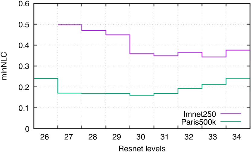
	single descriptor		PCA128	concatenation
	level	performance
ImageNet250	high (33)	0.376	0.353	0.323
Paris500k	low (30)	0.160	0.180	0.179

Figure 1: Top: discovery performance for k-means (minNLC, lower is better) as a function of the CNN activation level for the two evaluation datasets (ImageNet for classification and Paris500k for instance search). Bottom: impact of PCA dimensionality reduction and concatenation. See Section 4 for details on the datasets and the evaluation.

3.2 kNN graph construction on the GPU

Three of the four clustering algorithms we consider in this section use a matrix as input containing the similarity between all the images of the dataset. The graph matrix $A\in\mathbb{R}^{N\times N}$ is sparse and is equivalent to a kNN graph connecting each image to its neighbors, as determined by the similarity metric.

To construct the graph, we use a multi-GPU implementation of kNN search, implemented in the Faiss library Johnson et al. (2017). For small collections, i.e., up to 1 million images, we use a brute-force exact graph construction. For larger datasets, we use the Faiss IndexIVFFlat structure. Some Faiss search methods operate in the compressed domain, but we do not use them because they are slower on the GPU. Besides, since the memory usage is dominated by the matrix storage, we do not benefit from compression.

3.3 Clustering algorithms

We now introduce four clustering methods that we evaluate for the discovery task. The first is a regular k-means applied on the input descriptor. The three other ones use as input the sparse similarity matrix $A$, post-normalized with metric normalization and symmetrized, which amounts to adding $A^{\top}$ to $A$. The best normalization strategy depends on the method, but it typically involves a bandwidth parameter that controls the importance of weak versus strong edges. The key features of the algorithms are summarized in Table 1.

Algorithm	use graph	update variable	hyper-parameter	runtime (s)
k-means		centroids	k = 10000	21.3
AGC	x	node weights	$\tau=200000$	21.4 + 0.24
PIC	x	node weights	$\sigma=0.5$	21.4 + 0.35
MCL	x	edge weights	$r=1.4$	21.4 + 44.6

Table 1: Summary of the evaluated algorithms and their typical runtimes on ImageNet250 (300k images). Each algorithm has a parameter that sets the granularity of the clusters, we indicate its optimal value. For the methods that build upon the kNN graph, the graph construction time is added.

K-means.

We use the multi-GPU k-means implementation of Faiss. Performing a k-means on $N$ = $100$ million descriptors is fast compared to the step of extracting the descriptors with a ResNet. Our multi-GPU implementation produces the clusters in about 15 min with 8 Nvidia Titan X Maxwell GPUs, which we reduce to 4 min by sub-sampling the descriptors during the E-M iterations.

Agglomerative Clustering (AGC)

Agglomerative (or single-link) clustering depends only on the ordering of the edge weights. It removes edges that are below a given similarity threshold and identifies the connected components. Therefore, the weights must be globally comparable and a normalization pre-processing step is important. A simple similarity normalization Jégou et al. (2011) that updates each similarity by subtracting from it a similarity to a far away neighbor (the rank-50 nearest-neighbor) works the best in practice.

When swiping over the thresholds, a binary tree is generated where each cluster is a node and the two children of a node are two clusters at a finer granularity that were fused to produce the node. Any number of clusters $\tau$ can be obtained by stopping the agglomeration at a given threshold. A recent study Kontogianni et al. (2016) observes that such a single-link clustering tends to produce long chains. Our experiments in Section 4 concur with this observation.

Power Iteration Clustering (PIC)

Power iteration clustering finds a stationary distribution over the nodes of the graph by repeatedly multiplying a vector with the graph matrix until convergence. The actual clusters are typically extracted from the final distribution by clustering them in 1D Lin and Cohen (2010). However, this approach is hard to tune because it requires stopping the iterations before the clusters become indistinguishable. Therefore, we use a simple variant Cho and Lee (2012) where the clusters are identified by following the neighbors by a steepest ascent to a local maximum of the stationary distribution. Similar to other works Cho and Lee (2012), we found that a negative exponential to convert distances to weights $x\mapsto\exp(-x^{2}/\sigma^{2})$ produces the best results, with $\sigma$ controlling the bandwidth.

Markov Clustering (MCL)

This algorithm iterates over the similarity matrix as

$$A\leftarrow A\times A$$ (1)

$$A\leftarrow\Gamma_{r}(A)$$ (2)

where $\Gamma_{r}$ is an element-wise raising to power $r$ of the matrix, followed by a column-wise normalization Enright et al. (2002). The power $r\in(1,2]$ is the bandwidth parameter; when $r$ is high, small edges are reduced quickly along the iterations. A smaller $r$ preserves the edges longer. We found the matrix converges in 10-50 iterations. The clusters are read from the final matrix by extracting the connected components.

An important computational parameter is the sparsity of the matrix, determined by the number of non-zero elements of the matrix. After each $A\times A$ product, we use a global threshold on the matrix to force low elements to 0. If the matrix contains $kN$ non-zero elements, the storage and computational complexity of one iteration is $\mathcal{O}(Nk^{2})$. Because of this storage requirement, MCL is only applicable to relatively small collections (million-sized). To normalize $A$, we linearly map the rows of $A$ to the $[0,1]$ interval.

4 Experiments

This section describes our experiments carried out on the instance and category discovery tasks.

4.1 Datasets

dataset	# images	# labeled	# classes	class size (min/max)
ImageNet250	319512	319512	250	860/1300
Paris500k	501356	94303	79	114/22799
Flickr100M	95074575	0	0	N/A

Table 2: The three image datasets.

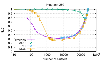
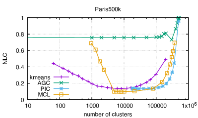
Figure 2: Comparison of clustering methods, in terms of NLC. By varying the hyper-parameters of Table 1, the number of clusters (x axis) can be adjusted.

We use 3 datasets in this study, see Table 2 for statistics.

ImageNet

We use ImageNet 2012 Dong et al. (2009) for evaluating the semantic discovery performance. We withhold the images from 750 classes (chosen at random) out of the 1000 to train the ResNet image descriptor. The ImageNet250 dataset is the set of classes that remain and used for evaluation of class discovery. The class sizes are balanced by design.

Paris500k

For the instance search dataset we use the Paris500k collection Weyand et al. (2010). It contains a set of Paris images from photo sharing sites, including landmarks, buildings, paintings, façades of cafés, etc. The authors did an extensive study of this dataset Weyand and Leibe (2015), with useful insights on the types of objects that appear in it, the reliability of geometrical matching, how to find representative images, etc. The dataset is partially labelled into classes, i.e. the unlabelled part of the dataset also contains instances of the classes.

YFCC100M

This dataset Thomee et al. (2016) contains 100 million representative images from the Flickr photo sharing site (we managed to download 95M of them). We use these images as distractors and consider them as unlabeled, even if some works have shown that the tags or GPS metadata can be used as weak supervision Joulin et al. (2016); Weyand et al. (2016). The images are diverse. A large fraction is portraits; there are also series of images from CCTV cameras.

Image description

The two image descriptors we employ are described in Section 3.1. We trained the ResNet on 750 classes on 4 Nvidia K40 GPUs during 3 days. The final top-1 error after 90 epochs is 26.5 %. To analyze the images, we resize all images to $244\times 244$ pixels and do a forward pass of the ResNet and keep activation maps of the layers we are interested in. Each minibatch of 128 images is processed in 670 ms on a K40.

Dataset bias

When combining datasets, it is important to be aware of the biases that define the datasets Torralba and Efros (2011). Some bias may cause the generation of dataset-uniform clusters, which makes the distractor set pointless. A priori, all images are mined from similar photo sharing sites (Flickr and Panoramio), but a different sampling or image preprocessing may introduce some bias as well.

We observe such a bias on the Paris dataset: many generated clusters were suspiciously pure clusters from Paris500k. To check this, we selected images from YFCC100M with the same selection criterion as Paris500k (on the GPS bounding box). Then we measured how the retrieval mAP for the labelled part of Paris500k decreased when adding distractors from Paris500k and Paris images selected from YFCC100M. The mAP decreases similarly, which shows that the only bias is due to the semantic content of the images.

4.2 Clustering performance evaluation

Given a reference clustering, there are several clustering performance measures that evaluate how similar the found clusters are to the ground truth classes (aka “reference clustering”). Classical measures include the normalized mutual information, cluster purity and rand index Lin and Cohen (2010).

Labelling cost, NLC and MinNLC

In this work, we choose the labelling cost (LC) as a performance measure. This cost was initially introduced by Guillaumin et al. for a face labelling task Guillaumin et al. (2009). It simulates the cost of an annotation interface that would be built on the given clustering. The annotator sees the clusters one after another, and can take two possible actions: (a) annotating the whole cluster of faces with a name, and (b) correcting the names of the faces of the cluster that are not the dominant identity of the cluster. The advantage of this measure is that it has a “physical” interpretation, and also offers an elegant way of selecting the tradeoff between under- and over-segmentation of the dataset. It is a cost, so lower is better. It is bounded by the the number of classes (lower bound, reached with a perfect clustering) and the number of images (upper bound, reached if each image gets a cluster).

To compare datasets of different sizes, we divide the LC by the number of images to annotate, yielding the normalized labelling cost (NLC). We often evaluate labelling costs for various clusterings that offer coarse-to-fine tradeoffs. In this case we report the minimum NLC over all cluster sizes (minNLC).

Precision and recall.

To compare with prior studies on the Paris dataset, we report the measures defined in the work by Weyand et al. Weyand et al. (2010), called precision and recall (somewhat misleadingly in a document retrieval context). Here, precision is computed as the number of images whose class is dominant in the cluster they are assigned to, normalized by the total number of images. This is related to cluster purity, but larger classes get a higher weight. The authors argue that this reflects applications where larger classes are simply more important. Recall is the dual of precision; it is the fraction of images that belong to the cluster that contains most images of their class. Achieving a high recall means that the images of a given class are not spread out over several clusters.

Handling distractors.

Distractors are unlabelled images that come from Paris500k and YFCC100M. They may or may not belong to one of the classes we are evaluating the clustering on. For our NLC measure we follow the practice of Weyand et al.  and the “junk” images for Oxford Building evaluation Philbin et al. (2007): we ignore the distractors in the computation of NLC. The measures are still relevant, because if many images with the same label are clustered together, it is likely that the unlabelled images of the cluster are also from the same class.

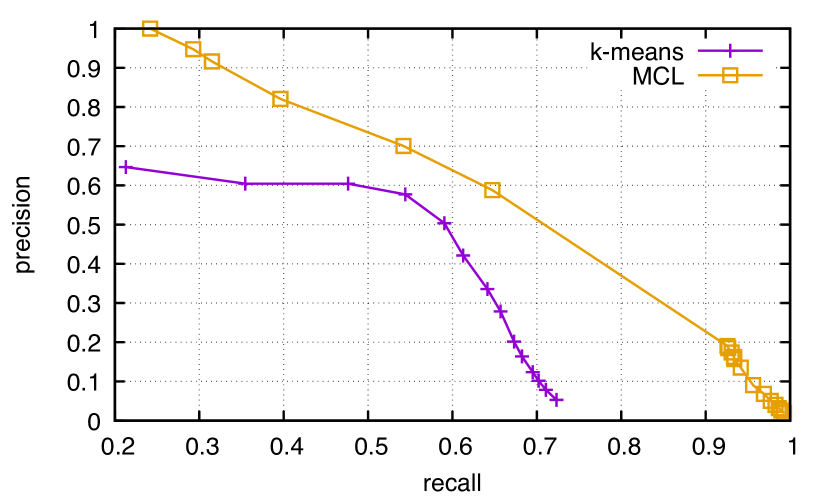
Figure 3: Precision vs. recall on the Paris dataset.

4.3 Results on the individual datasets

In Figure 2 we compare the clustering methods in terms of labelling cost, swiping different numbers of clusters. The first observation is that the NLC for Paris500k is much lower than that of ImageNet250, which reflects the fact that instance recognition is an easier task than image classification, for typical modern datasets. This is true despite the fact that the descriptors we use are close to the state of the art for image classification, but quite sub-optimal for instance search, since the R-MAC descriptions are extracted at a fixed resolution and without any fine-tuning of the convolutional part of the CNN Gordo et al. (2016); Radenović et al. (2016).

ImageNet250.

The MCL method is the clear winner, followed by k-means and PIC, while AGC gives very poor performance. The best performance is obtained for a number of clusters in between 1000 and 10000, which is larger than the number of categories of ImageNet250: it is easer for an annotator to label slightly over-segmented clusters than to dive into large clusters to individually label their contents.

Paris500k.

The ranking of methods is about the same as for ImageNet250. Note that for this dataset, the largest class is that of the Eiffel Tower, the best strategy when presented with a single cluster of all images is to label them all as Eiffel Tower (which is correct for 22% of the images), and correct the remaining images. This explains that the NLC is bounded at 0.78 for low numbers of clusters.

The clustering P-R is the standard performance measure for this dataset, and allows a direct comparison to previous studies. The performance that we achieve is lower than that reported in the original paper Weyand et al. (2010), which is expected since they use a full geometrical method and require a much more dense and costly comparison method.

The comparison to the results of Avrithis et al. Avrithis et al. (2015), which considers a more similar setup and is oriented towards efficient discovery, shows that our method obtains much better results (they have P-R operating points of around $(0.42,0.10)$). This is partly because we use a more powerful representation (ResNet rather than AlexNet), but also because our clustering method is better. More specifically, Figure 3 shows that MCL is significantly better than k-means in this instance discovery scenario. Our method is also faster, thanks to our better CPU and GPU implementations.

4.4 Balanced clusters

We analyze whether the four clustering methods produce balanced clusters in terms of size. Our measurements are carried on the ImageNet250 dataset, for which all classes have a very similar number of images. We would therefore have expected the different methods to produce balanced clusters.

It is in fact not the case: Figure 4 shows that k-means produces the most balanced clusters. For PIC and MCL about half of the clusters are singletons. The most unbalanced clustering is the agglomerative method. Its optimal operating point is at 200,000 clusters, which entails that 80 % of its clusters are singletons.

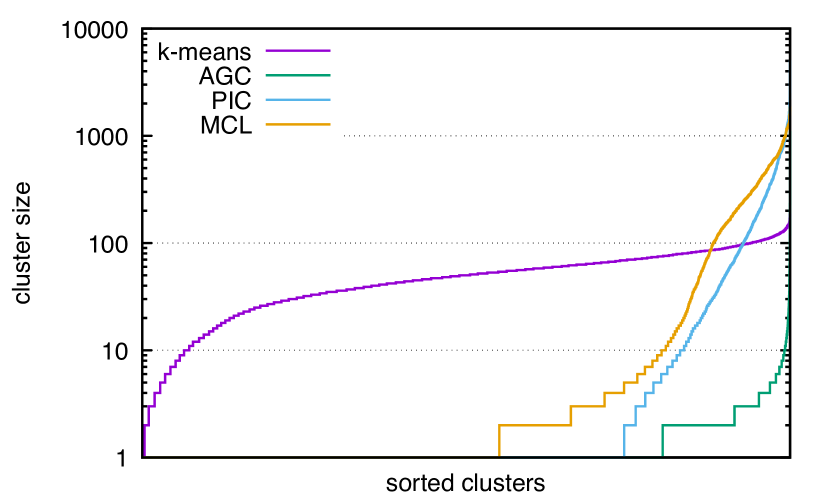
Figure 4: Sizes of the clusters produced by the clustering methods on ImageNet250, sorted from smallest to largest. The size of each clustering is chosen at the point where the minimum Labelling Cost is obtained.

4.5 Large-scale results

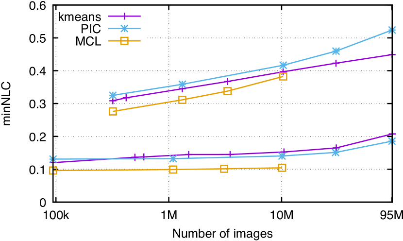
Figure 5: Clustering performance (minNLC, lower is better) as a function of number of distractors. The three curves above are for ImageNet250, the three below for Paris500k.

We combine ImageNet250 and Paris500k with a varying number of distractor images to evaluate the performance of the discovery on a large scale. Figure 5 reports the performance as a function of the dataset size. We do not experiment with AGC, which is clearly inferior. MCL is difficult to scale beyond 10M images: the squared matrix $A\times A$ has up to 13 billion edges, and the total memory usage is up to 120 GB. As expected, the performance degrades when the number of distractors increases. However, it degrades significantly slower for instance-level discovery than for class discovery. This is because the clusters have much clearer boundaries in the instance search case. In particular, MCL is almost not affected by distractors.

4.6 Visual results

We present examples of image clusters in Figures 6 and 7. The clusters are obtained by mixing both ImageNet250 and Paris500k with 95M images from YFCC100M. Recall that we rely on the visual content only to produce the clusters. To get an idea of how this could be combined with image tags to automatically label the clusters, we report the available annotations for the clusters: for ImageNet250 this is the synset name. For YFCC100M, we construct a bag of words (BoW) from the captions of the images of each cluster and report the most frequent words. The classes of Paris500k are not labelled.

Figure 6 shows that it is possible to propagate the ImageNet250 annotations to a whole cluster, or to find a more accurate name for animal species (dog $\leftrightarrow$ Bedlington terrier). For the Paris500k images, the BoW annotation gives a reliable name for the locations viewed in the images.

Figure 7 shows that there are many new clusters that also appear in the dataset. They are typically related to events (prom, concert), to objects that are not in the ImageNet collection (grafitti, fashion), or to combination of several classes occurring simultaneously in the cluster’s images.

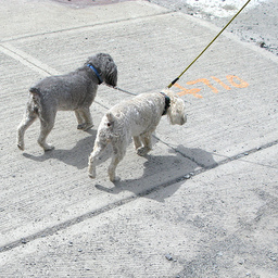
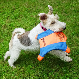
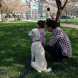
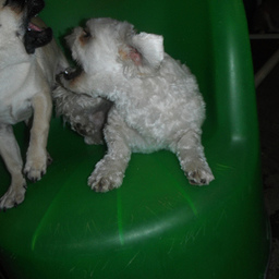
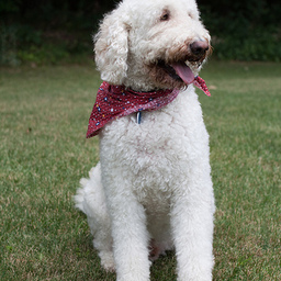
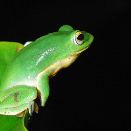
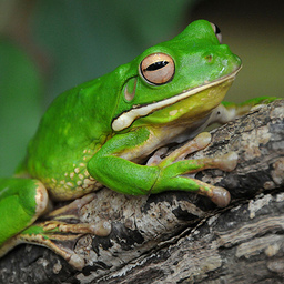
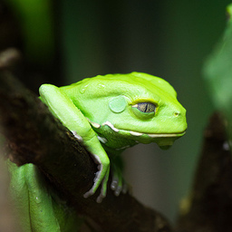
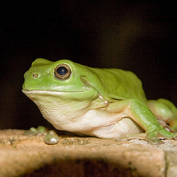
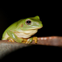
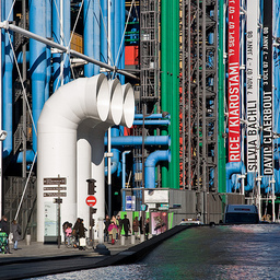
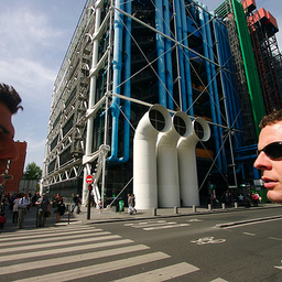
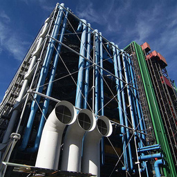
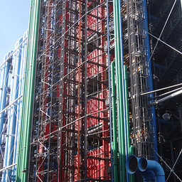
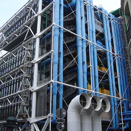
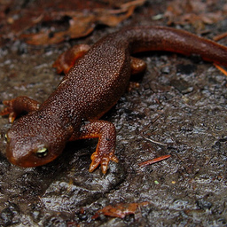
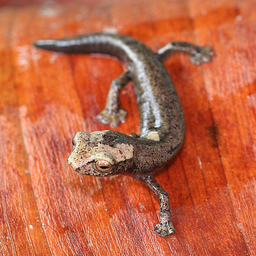
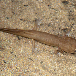
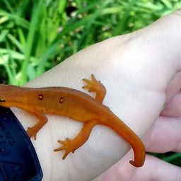
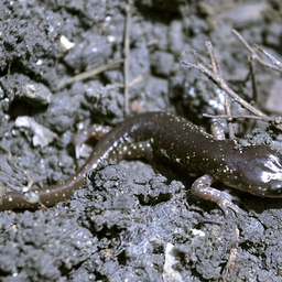
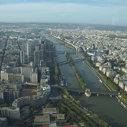
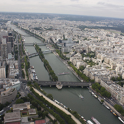
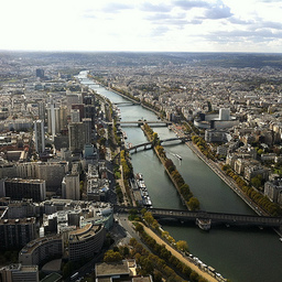
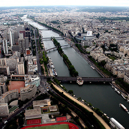
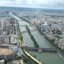
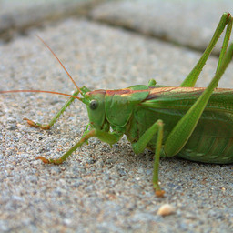
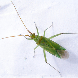
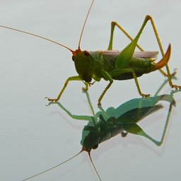
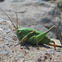
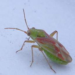
Size 3095 / BoW: 601*dog 265*dogs 259*poodle 182*park 128*puppy / Bedlington terrier
dugspr — Home for Good   Steve Guttman NYC   Patrise Henkel   Canine To Five   Big DumpTruck   Fabric-Guy  
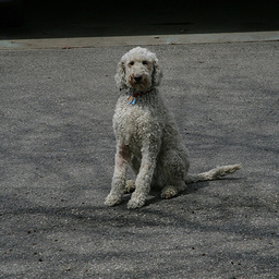
2691 / BoW: 948*frog 371*green 356*tree 200*zoo 195*frogs / tree frog, tree-frog
ansel117   Joachim S. Müller   Cloudtail   kobbe2008   IBI Productions   Eulinky  
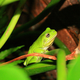
927 / BoW: 298*paris 246*pompidou 172*france 172*centre 59*georges
Peter Guthrie   Jeff_Werner   scarletgreen   Malcolm Payne   ciente   tobidope  
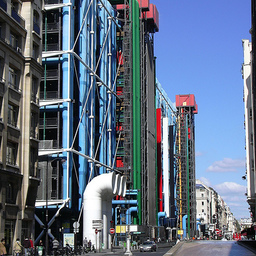
2374 / BoW: 359*salamander 253*lizard 228*newt 130*amphibian / common newt, Triturus vulgaris
jclor   Josiah Townsend   GregTheBusker   sam.davis.88   smashz   Todd W Pierson  
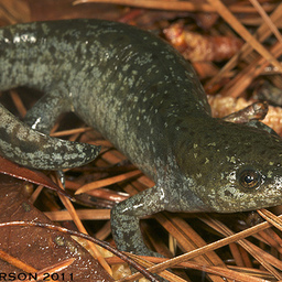
2515 / BoW: 349*view 339*tower 239*paris 178*france 165*city 157*chicago 145*eiffel 142*aerial 115*river 92*seine
tkaipi   rfzappala   Kimli   Peter Alfred Hess   Ulleskelf   sartak  
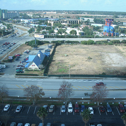
3480 / BoW: 817*macro 730*insect 572*grasshopper … 338*bug 313*heteroptera 282*mantis 261*katydid / lacewing, lacewing fly
Stinterwein   Mick E. Talbot   familynaturesummitpics   Jerry Friedman   Mick E. Talbot   Mick E. Talbot  

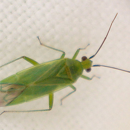
Figure 6: Example clusters with large intersections with a ground-truth category. For each cluster we indicate its size, the most frequent words from the Flickr annotations and the name of the ImageNet250 cluster with which it has the largest intersection. Although clusters contain Imagenet and Flickr500k images, we show only Flickr images for copyright reasons (and indicate the author’s name).

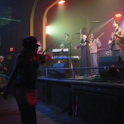
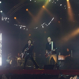
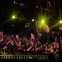
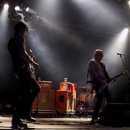
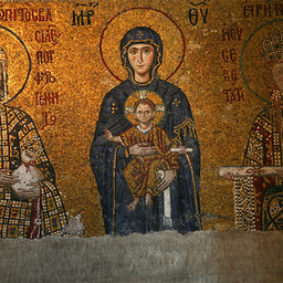
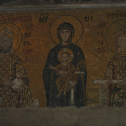
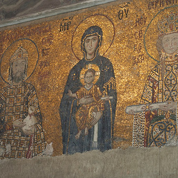
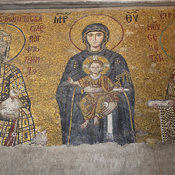
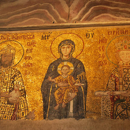
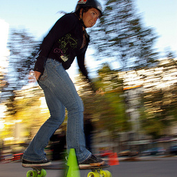
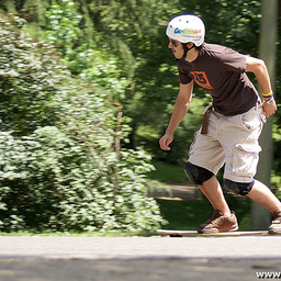
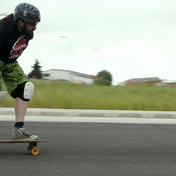
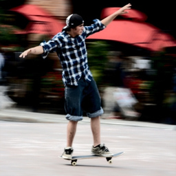
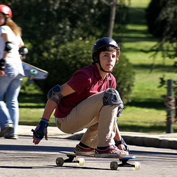
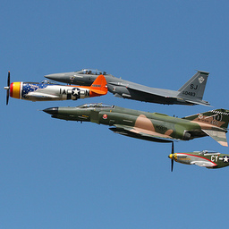
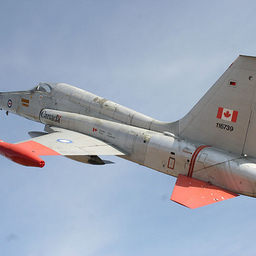
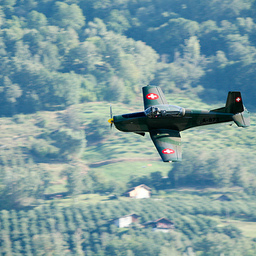
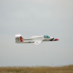
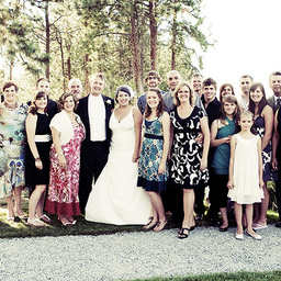
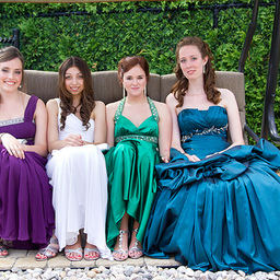
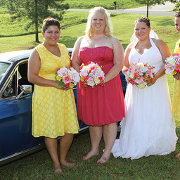
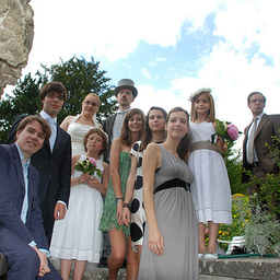
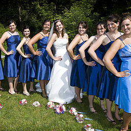
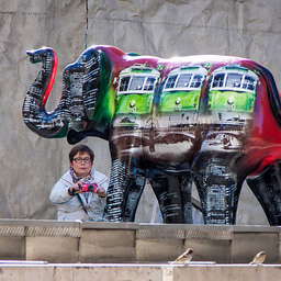
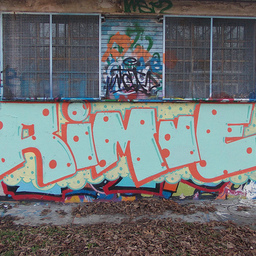
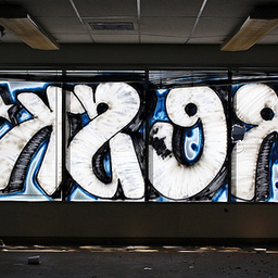
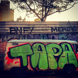
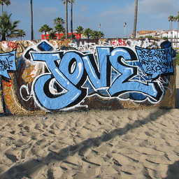
3981 / BoW: 867*concert 801*live 737*music 604*festival 375*rock 295*band
Agitproper   Ümloud!   Juan Seguí Moreno   Mattpl80   Adrián Pérez   Sean Molin Photography  
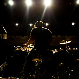
2247 / BoW: 767*istanbul 527*turkey 484*mosaic 449*hagia 445*sophia 234*church 193*aya 191*mosaics 189*italy 167*sofia
Edwin1710   felix.castor   nickcope   Te lo juro por Madonna   ana_ge   hp.weber  
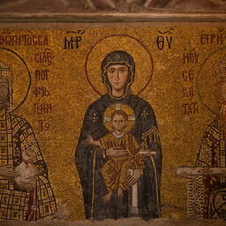
2413 / BoW: 1669*myprofe 1584*skate 1361*teacher 1361*language
Jsd_Quas0   Myprofe   Myprofe   Grégoire Lannoy   Myprofe   Daniel Dionne  
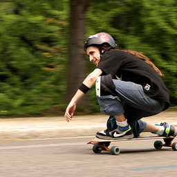
2547 / BoW: 687*air 509*aircraft 452*airshow 397*plane 365*airport 351*airplane 323*show
AV8PIX Christopher Ebdon   Feggy Art   Bobolink   Guillaume P. Boppe   gasmith   Ranger BP  
3398 / BoW: 1310*wedding 179*prom 135*bride 129*family 97*party
stephenjohnbryde   Keven Menard Photography   Josh Chretien   Christophe Porteneuve   Lake Effects Photography   rampion  
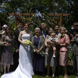
3370 / BoW: 1940*graffiti 742*art 583*street 327*urban 216*wall 190*streetart
vjpaul   en-ri   funkandjazz   Danilo Trombela   LosAnheles   Jason-Morrison  

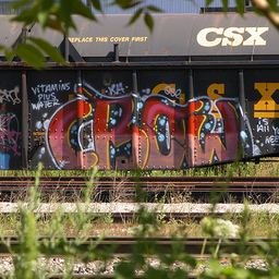
Figure 7: Example clusters without any specific intersection with a ground-truth category.

5 Conclusion

This paper presents a thorough evaluation of a large-scale discovery pipeline for both visual instances and categories. Our analysis of different clustering methods, distance normalizations, and descriptors shows that the best choices depend on the scale of the problem. The Markov Clustering algorithm offers the best quality but is scale-bounded because of the size of the affinity matrix. For large collections such as the YFCC100M dataset, Power Iteration Clustering and k-means are the best competitors.

Our experiments have been carried out with the novel and efficient multi-GPU implementations of the Faiss library, typically able to cluster 95 million images into 100,000 groups on one machine in less than 5 minutes. As a result, we report state-of-the-art results with respect to the trade-off between performance and efficiency.

Another conclusion is that category-level clusters can be improved by using lower-level descriptors. We plan to publish code and data that reproduce the experiments.

References

- [1]
- Agarwal et al. [2009] Sameer Agarwal, Noah Snavely, Ian Simon, Steven M Seitz, and Richard Szeliski. 2009. Building rome in a day. In CVPR. 72–79.
- Avrithis et al. [2015] Yannis Avrithis, Yannis Kalantidis, Evangelos Anagnostopoulos, and Ioannis Z Emiris. 2015. Web-scale image clustering revisited. In ICCV.
- Babenko and Lempitsky [2015] Artem Babenko and Victor Lempitsky. 2015. Aggregating local deep features for image retrieval. In CVPR. 1269–1277.
- Babenko et al. [2014] Artem Babenko, Anton Slesarev, Alexandr Chigorin, and Victor Lempitsky. 2014. Neural codes for image retrieval. In ECCV.
- Boaz Nadler and Kevrekidis [2008] Ronald R. Coifman Boaz Nadler, Stephane Lafon and Ioannis G. Kevrekidis. 2008. Diffusion maps, spectral clustering and reaction coordinates of dynamical systems. Technical Report. Arxiv.
- Cho et al. [2015] Minsu Cho, Suha Kwak, Cordelia Schmid, and Jean Ponce. 2015. Unsupervised Object Discovery and Localization in the Wild: Part-based Matching with Bottom-up Region Proposals. In CVPR.
- Cho and Lee [2012] Minsu Cho and Kyoung Mu Lee. 2012. Mode-seeking on graphs via random walks. In CVPR.
- Chum and Matas [2010] Ondrej Chum and Jiri Matas. 2010. Large-Scale Discovery of Spatially Related Images. IEEE Trans. PAMI 32, 2 (February 2010), 371–377.
- Dong et al. [2011] W. Dong, M. Charikar, and K. Li. 2011. Efficient K-Nearest Neighbor Graph Construction for Generic Similarity Measures. In WWW.
- Dong et al. [2009] Wei Dong, Richard Socher, Li Li-Jia, Kai Li, and Li Fei-Fei. 2009. ImageNet: A large-scale hierarchical image database. In CVPR.
- Donoser and Bischof [2013] Michael Donoser and Horst Bischof. 2013. Diffusion processes for retrieval revisited. In CVPR. 1320–1327.
- Enright et al. [2002] Anton J Enright, Stijn Van Dongen, and Christos A Ouzounis. 2002. An efficient algorithm for large-scale detection of protein families. Nucleic acids research 30, 7 (2002).
- Fergus et al. [2009] Rob Fergus, Yair Weiss, and Antonio Torralba. 2009. Semi-supervised learning in gigantic image collections. In NIPS. 522–530.
- Frahm et al. [2010] J.-M. Frahm, P. Georgel, D. Gallup, T. Johnson, R. Raguram, C. Wu, Y. Jen, E. Dunn, B. Clipp, S. Lazebnik, and M. Pollefeys. 2010. Building Rome on a Cloudless Day. In ECCV.
- Furon and Jégou [2013] Teddy Furon and Hervé Jégou. 2013. Using extreme value theory for image detection. Research Report RR-8244. INRIA.
- Golub and Loan [2013] Gene H Golub and Charles Van Loan. 2013. Matrix computations. John Hopkinks University Press.
- Gong et al. [2015] Yunchao Gong, Marcin Pawlowski, Fei Yang, Louis Brandy, Lubomir Bourdev, and Rob Fergus. 2015. Web scale photo hash clustering on a single machine. In Proceedings of the IEEE Conference on Computer Vision and Pattern Recognition. 19–27.
- Gong et al. [2014] Yunchao Gong, Liwei Wang, Ruiqi Guo, and Svetlana Lazebnik. 2014. Multi-scale orderless pooling of deep convolutional activation features. In ECCV.
- Gordo et al. [2016] Albert Gordo, Jon Almazan, Jerome Revaud, and Diane Larlus. 2016. Deep Image Retrieval: Learning Global Representations for Image Search. In ECCV.
- Guillaumin et al. [2009] Matthieu Guillaumin, Jakob Verbeek, and Cordelia Schmid. 2009. Is That You? Metric Learning Approaches for Face Identification. In IEEE International Conference on Computer Vision, 2009.
- Harwood and Drummond [2016] Ben Harwood and Tom Drummond. 2016. FANNG: Fast Approximate Nearest Neighbour Graphs. In CVPR.
- He et al. [2016] Kaiming He, Xiangyu Zhang, Shaoqing Ren, and Jian Sun. 2016. Deep residual learning for image recognition. CVPR (June 2016).
- Iscen et al. [2017a] Ahmet Iscen, Yannis Avrithis, Giorgos Tolias, Teddy Furon, and Ondrej Chum. 2017a. Fast Spectral Ranking for Similarity Search. arXiv preprint arXiv:1703.06935 (2017).
- Iscen et al. [2017b] Ahmet Iscen, Giorgos Tolias, Yannis Avrithis, Teddy Furon, and Ondrej Chum. 2017b. Efficient Diffusion on Region Manifolds: Recovering Small Objects with Compact CNN Representations. In CVPR.
- Jégou et al. [2011] Hervé Jégou, Matthijs Douze, and Cordelia Schmid. 2011. Exploiting descriptor distances for precise image search. Research Report RR-7656. INRIA.
- Jégou et al. [2007] Hervé Jégou, Hedi Harzallah, and Cordelia Schmid. 2007. A contextual dissimilarity measure for accurate and efficient image search. In CVPR.
- Johnson et al. [2017] Jeff Johnson, Matthijs Douze, and Hervé Jégou. 2017. Billion-scale similarity search with GPUs. arXiv preprint arXiv:1702.08734 (2017).
- Joulin et al. [2012] Armand Joulin, Francis Bach, and Jean Ponce. 2012. Multi-class cosegmentation. In CVPR. IEEE, 542–549.
- Joulin et al. [2016] Armand Joulin, Laurens van der Maaten, Allan Jabri, and Nicolas Vasilache. 2016. Learning Visual Features from Large Weakly Supervised Data. In ECCV.
- Kalantidis et al. [2016] Yannis Kalantidis, Lyndon Kennedy, Huy Nguyen, Clayton Mellina, and David A Shamma. 2016. LOH and behold: Web-scale visual search, recommendation and clustering using Locally Optimized Hashing. arXiv preprint arXiv:1604.06480 (2016).
- Kontogianni et al. [2016] Theodora Kontogianni, Markus Mathias, and Bastian Leibe. 2016. Incremental Object Discovery in Time-Varying Image Collections. In CVPR. 2082–2090.
- Lin and Cohen [2010] Frank Lin and William W Cohen. 2010. Power iteration clustering. In ICML.
- Lowe [2004] D. G. Lowe. 2004. Distinctive image features from scale-invariant keypoints. IJCV 60, 2 (2004), 91–110.
- Oliva and Torralba [2001] Aude Oliva and Antonio Torralba. 2001. Modeling the shape of the scene: a holistic representation of the spatial envelope. IJCV 42, 3 (2001), 145–175.
- Omercevic et al. [2007] D. Omercevic, O. Drbohlav, and A. Leonardis. 2007. High-dimensional feature matching: employing the concept of meaningful nearest neighbors. In ICCV.
- Perronnin et al. [2009] Florent Perronnin, Yan Liu, and J-M Renders. 2009. A family of contextual measures of similarity between distributions with application to image retrieval. In CVPR. 2358–2365.
- Philbin et al. [2007] J. Philbin, O. Chum, M. Isard, J. Sivic, and A. Zisserman. 2007. Object retrieval with large vocabularies and fast spatial matching. In CVPR.
- Philbin et al. [2008] J. Philbin, O. Chum, M. Isard, J. Sivic, and A. Zisserman. 2008. Lost in Quantization: Improving Particular Object Retrieval in Large Scale Image Databases. In CVPR.
- Philbin and Zisserman [2008] James Philbin and Andrew Zisserman. 2008. Object mining using a matching graph on very large image collections. In Computer Vision, Graphics & Image Processing.
- Radenović et al. [2016] Filip Radenović, Giorgos Tolias, and Ondřej Chum. 2016. CNN Image Retrieval Learns from BoW: Unsupervised Fine-Tuning with Hard Examples. In ECCV.
- Scheirer et al. [2012] Walter Scheirer, Neeraj Kumar, Peter Belhumeur, and Terrance Boult. 2012. Multi-attribute spaces: Calibration for attribute fusion and similarity search. In CVPR.
- Simonyan and Zisserman [2014] K. Simonyan and A. Zisserman. 2014. Very Deep Convolutional Networks for Large-Scale Image Recognition. arXiv preprint arXiv:1409.1556 (2014).
- Sivic and Zisserman [2003] Josef Sivic and Andrew Zisserman. 2003. Video Google: A Text Retrieval Approach to Object Matching in Videos. In ICCV. 1470–1477.
- Thomee et al. [2016] Bart Thomee, David A Shamma, Gerald Friedland, Benjamin Elizalde, Karl Ni, Douglas Poland, Damian Borth, and Li-Jia Li. 2016. YFCC100M: The new data in multimedia research. Commun. ACM 59, 2 (2016), 64–73.
- Tolias et al. [2013] Giorgios Tolias, Yannis Avrithis, and Hervé Jégou. 2013. To aggregate or not to aggregate: Selective match kernels for image search. In ICCV.
- Tolias et al. [2016] Giorgos Tolias, Ronan Sicre, and Hervé Jégou. 2016. Particular object retrieval with integral max-pooling of CNN activations. In ICLR.
- Torralba and Efros [2011] A. Torralba and A. A. Efros. 2011. Unbiased look at dataset bias. In CVPR.
- Weyand et al. [2010] Tobias Weyand, Jan Hosang, and Bastian Leibe. 2010. An evaluation of two automatic landmark building discovery algorithms for city reconstruction. In ECCV.
- Weyand et al. [2016] Tobias Weyand, Ilya Kostrikov, and James Philbin. 2016. Planet–photo geolocation with convolutional neural networks. In ECCV. Springer, 37–55.
- Weyand and Leibe [2015] Tobias Weyand and Bastian Leibe. 2015. Visual landmark recognition from internet photo collections: A large-scale evaluation. Computer Vision and Image Understanding 135 (2015), 1–15.
- Zeiler and Fergus [2014] M.D. Zeiler and R. Fergus. 2014. Visualizing and Understanding Convolutional Networks. In ECCV.
- Zelnik-Manor and Perona [2004] Lihi Zelnik-Manor and Pietro Perona. 2004. Self-tuning spectral clustering. NIPS 17, 1601-1608 (2004), 16.
- Zhao et al. [2013] Wan-Lei Zhao, Hervé Jégou, and Guillaume Gravier. 2013. Sim-Min-Hash: An efficient matching technique for linking large image collections. In ACM Multimedia.