Proximity-induced superconductivity in Landau-quantized graphene monolayers

Abstract

We consider massless Dirac fermions in a graphene monolayer in the ballistic limit, subject to both a perpendicular magnetic field $B$ and a proximity-induced pairing gap $\Delta$. When the chemical potential is at the Dirac point, our exact solution of the Bogoliubov-de Gennes equation yields $\Delta$-independent relativistic Landau levels. Since eigenstates depend on $\Delta$, many observables nevertheless are sensitive to pairing, e.g., the local density of states or the edge state spectrum. By solving the problem with an additional in-plane electric field, we also discuss how snake states are influenced by a pairing gap.

Introduction.—It is well known that at energies close to the neutrality point, the electronic properties of graphene monolayers are accurately described in terms of two-dimensional (2D) massless Dirac fermions Geim2004 ; Geim2005 ; Beenakker2008 ; CastroNeto2009 ; Goerbig2011 ; Andrei2012 ; Miransky2015 . Recent advances in fabrication and preparation technology Andrei2012 ; Dean2010 allow experimentalists to routinely reach the ballistic (disorder-free) transport regime. Our theoretical work reported below is largely motivated by spectacular recent progress on Josephson transport in ballistic graphene flakes contacted by conventional superconductors Calado2015 ; Lee2015 ; Allen2016 ; BenShalom2016 ; Efetov2016 ; Borzenets2016 ; Amet2016 ; Zhu2017 ; Nanda2017 ; Lee2017 ; Bretheau2017 , demonstrating in particular that proximity-induced superconductivity can coexist with rather high (Landau-quantizing) magnetic fields BenShalom2016 ; Amet2016 ; Lee2017 . This raises the question of how a proximity-induced bulk pairing gap will affect the electronic properties of graphene in an orbital magnetic field. In contrast to lateral graphene-superconductor interfaces, where theory is well developed Beenakker2008 ; Beenakker2006 ; Titov2006 ; Ossipov2007 , we therefore investigate vertical hybrid structures as shown schematically in Fig. 1. Superconductivity can be proximity-induced in the graphene sample from a 2D van der Waals superconductor Christian , e.g., using a NbSe₂ film supported on a standard hexagonal boron nitride (h-BN) substrate Dean2010 . NbSe₂ is a good superconductor with high critical field ($B_{c2}\approx 5$ T at $T=1$ K), remains superconducting down to a few monolayers, and exhibits high-quality interfaces with graphene Efetov2016 . For gating the device, another h-BN monolayer may be inserted as indicated in Fig. 1, at the expense of reducing the proximity gap. The proximitized graphene flake can be probed by a scanning tunneling microscope (STM), e.g., using a graphite finger tip for ultra-high energy resolution Bretheau2017 .

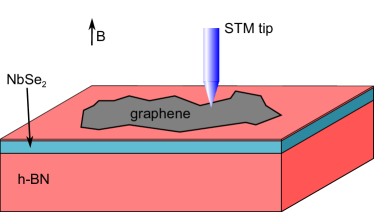
Figure 1: Sketch of a vertical hybrid structure in a perpendicular magnetic field $B$, where the graphene flake is deposited on a superconducting film (e.g., a few monolayers of NbSe₂) supported by an h-BN substrate. Inserting an h-BN monolayer between the superconductor and the graphene sample allows to gate the device (gates not shown). The graphene layer may be probed by an STM tip as indicated. Alternatively, the stack could be closed by a top h-BN monolayer.

Before turning to derivations, we briefly summarize our main results which can be tested by established STM techniques Zhao2015 , transport experiments, and/or local manipulation of defect charges in the substrate Lee2016 : (i) By means of an exact solution of the Bogoliubov-de Gennes (BdG) equation, we show that at the Dirac point, i.e., for chemical potential $\mu=0$, the energy spectrum of a proximitized graphene layer in a homogeneous magnetic field $B$ is independent of the proximity gap $\Delta$. The BdG spectrum thus reduces to the familiar relativistic Landau level spectrum CastroNeto2009 , in marked difference to the time-reversal-symmetric case with a strain-induced pseudo-magnetic field where the spectrum depends on $\Delta$ in a conventional manner Uchoa2013 ; Roy2014 ; LeeNandi2017 . (ii) Even though the energy spectrum is independent of $\Delta$ at the Dirac point, the corresponding eigenstates are sensitive to the pairing gap. Clear experimental signatures of proximity-induced superconductivity in Landau-quantized graphene are predicted for the energy-resolved local density of states (DOS) as well as for the edge states present near the sample boundaries. Away from the Dirac point, also the spectrum itself depends on $\Delta$. (iii) Chiral snake-like states are expected in graphene for $\Delta=0$ in the presence of a weak electric field $\cal E$ perpendicular to $B$ Lukose2007 ; Liu2015 ; Cohnitz2016 , see Refs. Tatch2015 ; Rickshaus2015 for recent experimental reports. We solve the corresponding BdG equation for arbitrary $\Delta$ through a Lorentz transformation of our solution for case (i), and thereby discuss how snake states are affected by a pairing gap.

Model.—We start from the BdG equation, $H\Psi=E\Psi$, for proximitized graphene samples as in Fig. 1. The BdG Hamiltonian is represented by the matrix Beenakker2008 ; Beenakker2006 ,

$$H=\left(\begin{array}[]{cc}v_{F}\left(\bm{\hat{p}}+\frac{e}{c}\bm{A}\right)\cdot\bm{\sigma}+V&\Delta\\ \Delta^{\ast}&-v_{F}\left(\bm{\hat{p}}-\frac{e}{c}\bm{A}\right)\cdot\bm{\sigma}-V\end{array}\right),$$ (1)

with canonical momentum $\bm{\hat{p}}=(\hat{p}_{x},\hat{p}_{y})=-i\hbar\bm{\nabla}$ and Fermi velocity $v_{F}\approx 10^{6}$ m$/$s. Pauli matrices $\sigma_{x,y}$ act in sublattice space, while explicitly written $2\times 2$ matrices refer to Nambu (particle-hole) space throughout. In particular, $H$ in Eq. (1) acts on Nambu spinors $\Psi({\bm{r}})=(u,v)^{T}$ containing the spin-up electron-like (spin-down hole-like) wave function $u$ ($v$) near the $K$ ($K^{\prime}$) valley, where $u$ and $v$ are spinors in sublattice space and ${\bm{r}}=(x,y)$. A decoupled identical copy of $H$ with opposite spin is kept implicit Beenakker2006 . The vector potential $\bm{A}=(0,Bx)$ describes a perpendicular homogeneous magnetic field $B$ in Landau gauge, where we neglect the typically small Zeeman splitting. The potential term in Eq. (1) also accounts for the chemical potential $\mu$ through the shift $V-\mu\to V$, and the homogeneous spin-singlet pairing amplitude $\Delta$ (taken real positive below) comes from the proximity effect. Note that intrinsic superconductivity in graphene Uchoa2007 ; Kopnin2008 has not been found experimentally. Finally, we neglect Coulomb interactions which are largely screened off by the proximity-inducing superconductor. In what follows, we measure lengths (wave numbers) in units of the magnetic length $l_{B}$ ($1/l_{B}$), and energies in units of the cyclotron scale $E_{B}$, where

$$l_{B}=\sqrt{\hbar c/eB},\quad E_{B}=\hbar v_{F}/l_{B}.$$ (2)

Equation (1) tacitly assumes applied magnetic fields below the critical field of the proximity-inducing superconductor and that the Meissner effect is too weak to completely expel the magnetic field from the proximitized graphene layer. In principle, renormalized values of $B$ and $\Delta$ entering Eq. (1) can be obtained from self-consistency equations, cf. Refs. Rasolt1992 ; MacDonald1993 . However, since coexistence of $B$ and $\Delta$ has already been observed in graphene BenShalom2016 ; Amet2016 ; Lee2017 and other 2D electron gases Nichele2017 , we here take them as effective parameters and focus on the physics caused by their interplay.

Chiral representation.—It is convenient to reformulate Eq. (1) using $4\times 4$ Dirac matrices in the chiral representation, $\beta=\left(\begin{array}[]{cc}0&-\sigma_{0}\\ -\sigma_{0}&0\end{array}\right)$ and $\alpha^{j}=\left(\begin{array}[]{cc}\sigma_{j}&0\\ 0&-\sigma_{j}\end{array}\right)$, with $j=1,2,3$ and identity $\sigma_{0}$ in sublattice space. Anticommuting $\gamma^{\nu}$ matrices are then given by $\gamma^{0}=\beta$ and $\gamma^{j}=\beta\alpha^{j}$, where we also define $\gamma^{5}={\rm diag}(\sigma_{0},-\sigma_{0})$. In Landau gauge, Eq. (1) is equivalently expressed as

$$H=\alpha^{1}\hat{p}_{x}+\alpha^{2}\left(\hat{p}_{y}+x\gamma^{5}\right)+\gamma^{5}V-\beta\Delta.$$ (3)

Formally, Eq. (3) describes 2D Dirac fermions with mass $-\Delta$ subject to pseudo-vector and pseudo-scalar potentials: the ${\bm{A}}$ and $V$ terms involve $\gamma^{5}$. Given a BdG eigenstate $\Psi_{E}=\left(u_{E},v_{E}\right)^{T}$ with energy $E\geq 0$, a particle-hole transformation yields a solution with energy $-E$,

$$\Psi_{-E}({\bm{r}})=-\gamma^{2}\Psi^{\ast}_{E}({\bm{r}})=\left(\begin{array}[]{c}-\sigma_{y}v_{E}^{*}({\bm{r}})\\ \sigma_{y}u_{E}^{*}({\bm{r}})\end{array}\right).$$ (4)

Therefore it is sufficient to find solutions with $E\geq 0$, and Eq. (4) is a self-conjugation relation for $E=0$. For a complete set $(u_{\lambda},v_{\lambda})^{T}$ with energies $E_{\lambda}\geq 0$, the local DOS $\rho(E)$ is defined in a standard way foot0 and can be measured by STM techniques, see Fig. 1, Furthermore, the charge current density ${\bm{J}}=(J_{x},J_{y})^{T}$ corresponding to a given eigenstate is

$${\bm{J}}_{\lambda}({\bm{r}})=-ev_{F}\left(u_{\lambda}^{\dagger}\bm{\sigma}u_{\lambda}+v_{\lambda}^{\dagger}\bm{\sigma}v_{\lambda}\right).$$ (5)

In what follows, we assume $V=V(x)$ such that Eq. (3) enjoys translation invariance along the $y$-direction. BdG solutions are given by $\Psi_{k}({\bm{r}})=e^{iky}\psi_{k}(x)$, where $\psi_{k}(x)$ is an eigenstate to $H_{k}$ obtained from $H$ in Eq. (3) with $\hat{p}_{y}\to k$. We now perform a partial (involving only the momentum in $y$-direction) Bogoliubov transformation, $\psi_{k}(x)=M_{k}\phi_{k}(x)$, with the unitary $4\times 4$ matrix

$$M_{k} = a_{k,+}-a_{k,-}\gamma^{2}=\left(\begin{array}[]{cc}a_{k,+}&-\sigma_{y}a_{k,-}\\ \sigma_{y}a_{k,-}&a_{k,+}\end{array}\right),$$

$$a_{k,\pm}=\sqrt{\frac{X_{k}\pm k}{2X_{k}}},\quad X_{k}=\sqrt{k^{2}+\Delta^{2}}.$$

The BdG equation, $\tilde{H}_{k}\phi_{k}(x)=E\phi_{k}(x)$ with $\tilde{H}_{k}=M_{k}^{-1}H_{k}M_{k}$, then involves the transformed Hamiltonian

$$\tilde{H}_{k}=\alpha^{1}\hat{p}_{x}+\alpha^{2}\left(X_{k}+x\gamma^{5}\right)+\frac{k+\gamma^{2}\Delta}{X_{k}}\gamma^{5}V(x).$$ (9)

For $B=0$ and constant $V$, one has plane waves with ${\bm{k}}=(k_{x},k)$ and energy $E_{{\bm{k}},\pm}=\sqrt{(\pm\hbar v_{F}|{\bm{k}}|+V)^{2}+\Delta^{2}}$ Beenakker2006 , where the DOS for $E\geq 0$ and $V\geq 0$ is given by

$$\rho(E)=\frac{1}{\pi(\hbar v_{F})^{2}}\times\left\{\begin{array}[]{cc}0,&E<\Delta,\\ \frac{EV-(E^{2}-\Delta^{2})}{\sqrt{E^{2}-\Delta^{2}}},&\Delta<E<\sqrt{V^{2}+\Delta^{2}},\\ E-V,&E>\sqrt{V^{2}+\Delta^{2}}.\end{array}\right.$$ (10)

Note that at the Dirac point, i.e., for $V=0$, the usual BCS square-root singularity is replaced by a finite jump at $E=\Delta$, with $\rho(E)\sim E$ for $E>\Delta$.

Exact solution at the Dirac point.—For $V=0$, we next observe that $\tilde{H}_{k}$ in Eq. (9) coincides with the original Hamiltonian in Eq. (3) for $\Delta=0$ and $\hat{p}_{y}\to X_{k}$. As a consequence, the entire spectrum coincides with the $(k,\Delta)$-independent relativistic Landau energies, $E_{k,n,s}=E_{n}=\sqrt{2n}E_{B}$ with $n=0,1,2,\ldots$ CastroNeto2009 . On top of the $k$-degeneracy, we have an additional double degeneracy with $s=\pm$, see below. Eigenstates follow by the above $M_{k}$ transformation from relativistic Landau states. The latter are given by the Nambu spinors $\phi_{k,n,+}(x)=\left({\cal F}_{n}(x+X_{k}),0\right)^{T}$ and $\phi_{k,n,-}(x)=\left(0,\sigma_{y}{\cal F}_{n}(x-X_{k})\right)^{T}$, where sublattice spinors, ${\cal F}_{n}(x)=(\frac{1}{\sqrt{2}})^{1-\delta_{n,0}}\left({\rm sgn}(n)\varphi_{|n|-1},i\varphi_{|n|}\right)^{T}$, are expressed in terms of normalized oscillator eigenfunctions foot1 . Note that the usual center-of-mass coordinate $k$ is replaced by $X_{k}$ ($-X_{k}$) for the electron (hole) spinor component, cf. Eq. (9). Using Eq. (Proximity-induced superconductivity in Landau-quantized graphene monolayers), eigenstates follow as

$$\Psi_{k,n,s=\pm}({\bm{r}})=e^{iky}\left(\begin{array}[]{c}\pm a_{k,\pm}{\cal F}_{n}(x\pm X_{k})\\ a_{k,\mp}\sigma_{y}{\cal F}_{n}(x\pm X_{k})\end{array}\right).$$ (11)

In contrast to the spectrum, these states depend on $\Delta$ and thus most observables will be sensitive to pairing. For given $\Psi_{k,n,s}$, Eq. (4) yields a mirror state $\Psi_{-k,-n,\pm}({\bm{r}})=\pm\gamma^{2}\Psi^{*}_{k,n,\pm}({\bm{r}})$ with $E=-E_{n}$. For $n=0$, this relation connects $+k$ and $-k$ states, and one can construct two ($s=\pm$) 1D zero-energy Majorana fields.

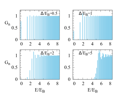
Figure 2: Bar plots of the DOS weights $G_{n}$ vs Landau energy $E_{n}$ for different $\Delta/E_{B}$, see Eqs. (Proximity-induced superconductivity in Landau-quantized graphene monolayers) and (13).

Density of states at the Dirac point.—By using the states in Eq. (11) and restoring units, we obtain an exact integral representation for the DOS SM ,

$$\rho(E) = \frac{e^{-(\Delta/E_{B})^{2}}}{\pi l_{B}^{2}}\delta(E)+\frac{|E|}{\pi(\hbar v_{F})^{2}}\times$$

$$\times \int_{-\infty-i0^{+}}^{+\infty-i0^{+}}\frac{d\lambda}{2\pi i}e^{i(E^{2}\lambda-\Delta^{2}\tan\lambda)/E_{B}^{2}}\cot\lambda,$$

which is singular and applies in the distribution sense. For $B\to 0$, the asymptotic approximation of Eq. (Proximity-induced superconductivity in Landau-quantized graphene monolayers) reproduces Eq. (10) with $V=0$. The bar plots in Fig. 2 show the dimensionless DOS weights

$$G_{n}=\pi l_{B}^{2}\int_{E_{n}-0^{+}}^{E_{n}+0^{+}}dE\rho(E),\quad E_{n}=\sqrt{2n}E_{B},$$ (13)

characterizing the $\delta(|E|-E_{n})$ peaks in the DOS and hence also the degeneracy per unit area of the energy levels $E_{n}$. For $\Delta\to 0$, Eq. (Proximity-induced superconductivity in Landau-quantized graphene monolayers) yields the standard Landau comb with $G_{n}=1$. Figure 2 illustrates the crossover between the analytically accessible limits $\Delta/E_{B}\to 0$ and $\Delta/E_{B}\to\infty$, where low-energy states with $|E|<\Delta$ become gradually depleted as $\Delta/E_{B}$ increases. The DOS in Fig. 2 also exhibits oscillatory features in the energy dependence.

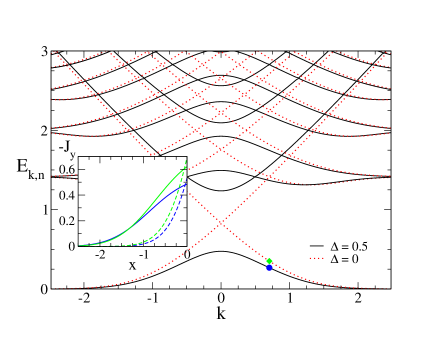
Figure 3: Edge states for a semi-infinite ($x<0$) graphene sheet with $V=0$ and armchair conditions at $x=0$. Main panel: Dispersion relation for $\Delta=0.5E_{B}$ (solid black) and for $\Delta=0$ (red dotted curves). Inset: Current density $J_{y}(x)$ [in units of $-ev_{F}$] vs position $x/l_{B}$ for the two degenerate eigenstates (solid and dashed curves for $s=+$ and $s=-$, resp.) with $kl_{B}=0.705$. Blue (green) curves are for $\Delta/E_{B}=0.5$ ($\Delta=0$) with $E_{k,n,s}/E_{B}\simeq 0.2683$ ($\simeq 0.3520$), cf. the blue circle (green diamond) in the main panel.

Edge states.—Next we consider a semi-infinite graphene sheet ($x<0$) with $V=0$. The boundary is modeled by imposing armchair conditions Beenakker2008 ; CastroNeto2009 along the line $x=0$. Solutions to the BdG equation are then given in terms of parabolic cylinder functions $D_{p}(z)$ Abramowitz . The spectrum is obtained by numerically solving ${\rm det}[{\bm{W}}(E)]=0$, where the matrix ${\bm{W}}$ follows with $\epsilon=E/\sqrt{2}$, $a_{\pm}=a_{k,\pm}$ [cf. Eq. (Proximity-induced superconductivity in Landau-quantized graphene monolayers)], and $\tilde{D}_{p}^{(\pm)}=D_{p}\left(\pm\sqrt{2(k^{2}+\Delta^{2})}\right)$ in the form SM

$$\left(\begin{array}[]{cccc}-a_{+}\epsilon\tilde{D}_{\epsilon^{2}-1}^{(-)}&a_{+}\tilde{D}_{\epsilon^{2}}^{(-)}&a_{-}\epsilon\tilde{D}_{\epsilon^{2}-1}^{(+)}&a_{-}\tilde{D}_{\epsilon^{2}}^{(+)}\\ a_{+}\tilde{D}_{\epsilon^{2}}^{(-)}&-a_{+}\epsilon\tilde{D}_{\epsilon^{2}-1}^{(-)}&-a_{-}\tilde{D}_{\epsilon^{2}}^{(+)}&-a_{-}\epsilon\tilde{D}_{\epsilon^{2}-1}^{(+)}\\ a_{-}\tilde{D}_{\epsilon^{2}}^{(-)}&-a_{-}\epsilon\tilde{D}_{\epsilon^{2}-1}^{(-)}&a_{+}\tilde{D}_{\epsilon^{2}}^{(+)}&a_{+}\epsilon\tilde{D}_{\epsilon^{2}-1}^{(+)}\\ a_{-}\epsilon\tilde{D}_{\epsilon^{2}-1}^{(-)}&-a_{-}\tilde{D}_{\epsilon^{2}}^{(-)}&a_{+}\epsilon\tilde{D}_{\epsilon^{2}-1}^{(+)}&a_{+}\tilde{D}_{\epsilon^{2}}^{(+)}\end{array}\right)$$ (14)

The spectrum is shown in Fig. 3. For $\Delta=0$, we recover earlier results Brey2006 ; Abanin2007 ; Delplace2010 reporting chiral edge states. For $\Delta>0$, electron- and hole-type edge states become mixed and the edge state dispersion exhibits gaps near $k=0$. Turning to the current density (5), the current flows along the $y$-direction only, $J_{x}=0$. The respective profile, $J_{y}(x)$, is illustrated for the two degenerate states with $k=0.705$ and lowest energy in the inset of Fig. 3. Since the current density has a pronounced peak near $x=0$ and a specific sign, we have unidirectional edge states also for $\Delta>0$. However, the overall current becomes smaller with increasing $\Delta$, cf. Fig. 3.

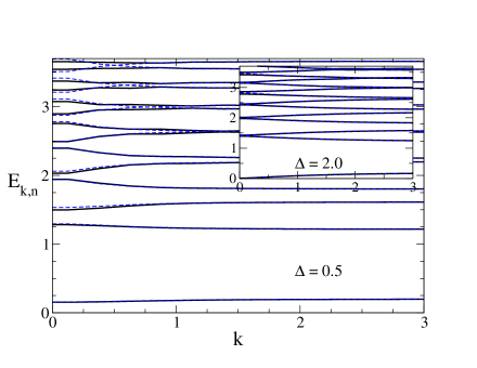
Figure 4: Dispersion relation for an infinite graphene sheet with potential $V=0.2E_{B}$ for $\Delta=0.5E_{B}$ (main panel) and $\Delta=2E_{B}$ (inset). Since $E_{-k,n}=E_{k,n}$, only $k\geq 0$ is shown. Solid black and dashed blue curves refer to numerical diagonalization and perturbative results [Eq. (15)], respectively.

Going away from the Dirac point.—Let us briefly address the case $V\neq 0$, where numerical diagonalization of the BdG equation using Landau states as basis shows that a (chemical) potential shift causes dispersion, see Fig. 4. Notably, most features in Fig. 4 can be understood by expanding around the $V=0$ solution (11) using the term $\sim V$ in Eq. (9) as small perturbation. Writing $E_{k,n,s}=E_{n}+\delta E_{k,n,s}$, first-order degenerate perturbation theory yields the correction

$$\delta E_{k,n,\pm}=\pm\frac{|V|}{X_{k}}\sqrt{k^{2}+\Delta^{2}S^{2}_{k,n}},$$ (15)

where the overlap between Landau states ${\cal F}_{n}$ centered at $+X_{k}$ and $-X_{k}$ is encoded by $S_{k,n}$. Explicitly, we find $S_{k,0}=e^{-X_{k}^{2}}$ and $S_{k,n>0}=\frac{1}{2}e^{-X_{k}^{2}}[L_{n-1}(2X_{k}^{2})+L_{n}(2X_{k}^{2})]$ with the Laguerre polynomials $L_{n}$ Abramowitz . For $|k|\gg\Delta$, Eq. (15) yields a uniform shift $\pm|V|$ of all Landau energies, while for $k=0$, the correction simplifies to $\pm|VS_{0,n}|$, where $S_{0,n}$ oscillates when changing $n$.

Crossed electric and magnetic fields.—We finally also include an in-plane electric field ${\cal E}$ by putting $V=e{\cal E}x$. With the dimensionless parameter $\varepsilon=(c/v_{F}){\cal E}/B$, we consider the regime $|\varepsilon|<1$. The corresponding $\Delta=0$ problem has been solved analytically by a Lorentz boost into the reference frame with vanishing electric field (${\cal E}^{\prime}=0)$ Lukose2007 . Remarkably, such a strategy also admits an exact solution for $\Delta\neq 0$: First, we write down the spinor transformation law, $\psi=S\psi^{\prime}$ with $S=\cosh(\eta/2)-\sinh(\eta/2)\gamma^{0}\gamma^{2}$, where the Lorentz angle $\eta=\tanh^{-1}\varepsilon$ defines the frame with ${\cal E}^{\prime}=0$. Next, using the parameter $\zeta\equiv(1-\varepsilon^{2})^{1/4}$, we rescale (i) the $x$-coordinate, $x^{\prime}=\zeta x$, (ii) the wave number, $k^{\prime}=(k+\varepsilon E)/\zeta^{3}$, (iii) energy, $E^{\prime}=(E+\varepsilon k)/\zeta^{3}$, and (iv) the proximity gap, $\Delta^{\prime}=\Delta/\zeta$. With these rescalings and $X_{k}^{\prime}=\sqrt{k^{\prime 2}+\Delta^{\prime 2}}$, cf. Eq. (Proximity-induced superconductivity in Landau-quantized graphene monolayers), the BdG equation in the new frame coincides with the $V=0$ problem solved above. Transforming the solution, Eq. (11), back to the lab frame and restoring units, we obtain the $\Delta$-independent spectrum

$$E_{k,n,s}=-\hbar\varepsilon v_{F}k+{\rm sgn}(n)\sqrt{2|n|}\zeta^{3}E_{B},$$ (16)

where $n$ runs over all integers and $k$ is restricted to those values with $E_{k,n,s}\geq 0$. Each level is two-fold degenerate ($s=\pm$), and the corresponding eigenstates are

$$\Psi_{k,n,\pm}({\bm{r}}) = e^{iky}\zeta^{3/2}\Biggl{[}\cosh(\eta/2)\left(\begin{array}[]{c}\pm a_{k^{\prime},\pm}{\cal F}_{n}(x^{\prime}\pm X_{k}^{\prime})\\ a_{k^{\prime},\mp}\sigma_{y}{\cal F}_{n}(x^{\prime}\pm X^{\prime}_{k})\end{array}\right)$$ (19)

$$+ \sinh(\eta/2)\left(\begin{array}[]{c}\mp a_{k^{\prime},\pm}\sigma_{y}{\cal F}_{n}(x^{\prime}\pm X^{\prime}_{k})\\ a_{k^{\prime},\mp}{\cal F}_{n}(x^{\prime}\pm X^{\prime}_{k})\end{array}\right)\Biggr{]},$$ (22)

States with negative energy follow from Eq. (4), and for $\varepsilon=0$, Eq. (22) reduces to Eq. (11).

In the normal ($\Delta=0$) case, so-called snake states exist near the interface between $V>0$ and $V<0$ regions Liu2015 ; Cohnitz2016 ; Tatch2015 ; Rickshaus2015 which are semiclassically described by snake-like orbits propagating along the interface (here the $y$-direction) with velocity $c{\cal E}/B=\varepsilon v_{F}$. In the superconducting case ($\Delta>0$), the spectrum in Eq. (16) suggests that unidirectional snake states remain well defined and propagate with the same snake velocity as for $\Delta=0$. In particular, for $n=0$, these states are localized near the line $x=0$. Computing the total charge current carried by a given state along the $y$-direction, $I=\int dxJ_{y}(x)$, Eqs. (5) and (22) yield the analytical result $I(\Delta)/I(0)=1/\sqrt{1+(\Delta^{\prime}/k^{\prime})^{2}}$. Similar to the above edge state case, we thus find that the magnitude of the current becomes gradually suppressed with increasing $\Delta$.

Conclusions.—We have studied electronic properties of graphene monolayers in an orbital magnetic field when also proximity-induced pairing correlations are present. Remarkably, at the Dirac point, the energy spectrum is independent of $\Delta$, but observables may still show pronounced pairing effects since eigenstates depend on $\Delta$. We hope that our work will stimulate experimental and further theoretical work on the coexistence of magnetism and superconductivity in graphene.

Appendix A Density of states at Dirac point

We first discuss the derivation of Eq. (10) in the main text. Below we set $a=\Delta/E_{B}$. Using the exact $V=0$ states in Eq. (9), the local DOS takes the form

$$\rho(E) = 2g_{0}\delta(E)+\sum_{n>0}(g_{n-1}+g_{n})\delta\left(|E|-\sqrt{2n}E_{B}\right),$$

$$g_{n} = \int\frac{dk}{2\pi}\varphi^{2}_{n}\left(\sqrt{(kl_{B})^{2}+a^{2}}\right)=\frac{1}{2\pi l_{B}^{2}}I_{n}(a),$$ (23)

$$I_{n}(a) = \frac{1}{\sqrt{\pi}2^{n}n!}\int_{a^{2}}^{\infty}\frac{du}{\sqrt{u-a^{2}}}H^{2}_{n}\left(\sqrt{u}\right)e^{-u}.$$

For $\Delta=0$, we have $I_{n}(0)=1$ and the Landau comb is reproduced. Moreover, $I_{0}(a)$ yields the $\delta(E)$ prefactor in Eq. (10). We thus focus on the local DOS for $|E|>0$. With $D$ denoting an effective high-energy bandwidth, where eventually the limit $D\to\infty$ has to be taken, we can rewrite Eq. (23) as

$$\rho(E)=\frac{1}{2\pi l^{2}_{B}}\sum_{n>0}e^{-2n(E_{B}/D)^{2}}\left[I_{n-1}(a)+I_{n}(a)\right]\times$$

$$\qquad\qquad\qquad\times\ \delta\left(|E|-\sqrt{2n}E_{B}\right)$$ (24)

$$=\frac{|E|}{\pi l^{2}_{B}}\sum_{n>0}(I_{n-1}+I_{n})e^{-2n(E_{B}/D)^{2}}\int_{-\infty}^{+\infty}\frac{d\lambda}{2\pi}e^{i\lambda(E^{2}-2nE^{2}_{B})}$$

with $\delta(E^{2}-2nE_{B}^{2})=(2|E|)^{-1}\delta(|E|-\sqrt{2n}E_{B})$ and an integral representation of the $\delta$-function. Exchanging sum and integral, measuring $E$ in units of $\Delta$ and rescaling $\lambda\to\lambda/\Delta^{2}$, we find

$$\rho(E) = \frac{\Delta|E|}{\pi(\hbar v_{F})^{2}}e^{-(E/\tilde{D})^{2}}\times$$

$$\times \int_{-\infty}^{+\infty}\frac{d\lambda}{2\pi a^{2}}e^{i\tilde{\lambda}E^{2}}\left(e^{-2i\tilde{\lambda}}+1\right){\cal G}_{a}(\tilde{\lambda}),$$

where we define $\tilde{D}=D/\Delta$,

$${\cal G}_{a}(\tilde{\lambda})=\sum_{n\geq 0}I_{n}(a)e^{-2i\tilde{\lambda}n},\quad\quad\tilde{\lambda}=\frac{1}{a^{2}}\left(\lambda-\frac{i}{\tilde{D}^{2}}\right).$$

Next, using $\left|e^{-2i\tilde{\lambda}}\right|<1$ and the Poisson kernel Abramowitz , we sum up the series,

$${\cal G}_{a}(\tilde{\lambda}) = \sum_{n\geq 0}\frac{1}{\sqrt{\pi}}\int_{a^{2}}^{\infty}\frac{du}{\sqrt{u-a^{2}}}\frac{H^{2}_{n}(\sqrt{u})}{2^{n}n!}e^{-u}e^{-2i\tilde{\lambda}n}$$ (26)

$$= \frac{1}{\sqrt{\pi}}\int_{a^{2}}^{\infty}\frac{du}{\sqrt{u-a^{2}}}\frac{\exp\left(u\frac{2e^{-2i\tilde{\lambda}}}{1+e^{-2i\tilde{\lambda}}}\right)}{(1-e^{-4i\tilde{\lambda}})^{1/2}}e^{-u}$$

$$= \frac{1}{1-e^{-2i\tilde{\lambda}}}\exp\left(-\frac{1-e^{-2i\tilde{\lambda}}}{1+e^{-2i\tilde{\lambda}}}a^{2}\right).$$

Inserting Eq. (26) into Eq. (A), we obtain

$$\rho(E)=\frac{\Delta|E|}{\pi(\hbar v_{F})^{2}}e^{-(E/\tilde{D})^{2}}\times$$

$$\quad\times\int_{-\infty-i/\tilde{D}^{2}}^{+\infty-i/\tilde{D}^{2}}\frac{d\lambda}{2\pi i}\frac{e^{i\lambda E^{2}-a^{2}\tan(\lambda/a^{2})}}{a^{2}\tan(\lambda/a^{2})}.$$ (27)

Restoring units, letting $D\to\infty$, and including the $E=0$ peak, we arrive at Eq. (10) in the main text.

Appendix B On the determinantal condition

We here consider the semi-infinite case ($x<0$) with $V=0$ and armchair boundary conditions imposed on the line $x=0$. For given wave number $k$ and energy $E$, using the parabolic cylinder functions $D_{p}(z)$ Abramowitz , general solutions of the BdG equation that are normalizable for $x<0$ are given by the Nambu spinors

$$\Psi_{k,E}({\bm{r}}) = c_{1}e^{iky}\left(\begin{array}[]{c}a_{+}{\cal F}_{X_{k},E}(x)\\ a_{-}\sigma_{y}{\cal F}_{X_{k},E}(x)\end{array}\right)+$$ (30)

$$+ c_{2}e^{iky}\left(\begin{array}[]{c}-a_{-}{\cal F}_{-X_{k},E}(x)\\ a_{+}\sigma_{y}{\cal F}_{-X_{k},E}(x)\end{array}\right),$$ (33)

with complex coefficients $c_{1,2}$, the numbers $a_{\pm}\equiv a_{k,\pm}$ in Eq. (6), and the sublattice spinors ($p\equiv E^{2}/2$)

$${\cal F}_{\pm X_{k},E}(x)=\left(\begin{array}[]{c}-\frac{E}{\sqrt{2}}D_{p-1}\left(-\sqrt{2}(x\pm X_{k})\right)\\ iD_{p}\left(-\sqrt{2}(x\pm X_{k})\right)\end{array}\right).$$ (34)

We now impose armchair boundary conditions at $x=0$,

$$\psi_{A}(0,y)+\psi^{\prime}_{A}(0,y)=0,\quad\psi_{B}(0,y)+\psi^{\prime}_{B}(0,y)=0,$$ (35)

where the sublattice spinor components $\psi_{A/B}({\bm{r}})\ [\psi^{\prime}_{A/B}({\bm{r}})]$ characterize an electron at the $K$ [$K^{\prime}$] valley and Eq. (35) has to be satisfied for all $y$. Next we note that the upper Nambu spinor component in Eq. (30) contains $\psi_{A/B}({\bm{r}})$ for an electron at the $K$ valley with wave number $k$ and energy $E$, while the lower component of Eq. (30) contains the complex conjugate of $\psi^{\prime}_{A/B}({\bm{r}})$ for an electron at the $K^{\prime}$ valley with wave vector $-k$ and energy $-E$. In order to satisfy Eq. (35), we thus have to consider superpositions of $\pm k$ states with the same energy $E$. Using complex coefficients $d^{*}_{1,2}$ to parametrize the partner states with wave number $-k$ and the same energy $E$, see Eq. (30), and using ${\cal F}^{*}_{\pm X_{k},-E}=-{\cal F}_{\pm X_{k},E}$, Eq. (35) yields the relations

$$c_{1}a_{+}{\cal F}_{X_{k},E}-c_{2}a_{-}{\cal F}_{-X_{k},E}$$ (36)

$$+\ d_{1}a_{+}\sigma_{y}{\cal F}_{X_{k},E}+d_{2}a_{-}\sigma_{y}{\cal F}_{-X_{k},E}=0,$$

$$c_{1}a_{-}\sigma_{y}{\cal F}_{X_{k},-E}+c_{2}a_{+}\sigma_{y}{\cal F}_{-X_{k},-E}$$

$$-\ d_{1}a_{-}{\cal F}_{X_{k},-E}+d_{2}a_{+}{\cal F}_{-X_{k},-E}=0,$$

where all sublattice spinors ${\cal F}$ are taken at $x=0$. The relations (36) result in four equations for the four variables ($c_{1},d_{1},c_{2},d_{2}$). We thus arrive at the matrix ${\bm{W}}(E)$ in Eq. (12). For $\Delta=0$, the corresponding determinantal condition simplifies to $pD_{p-1}^{2}(-\sqrt{2}k)=D_{p}^{2}(-\sqrt{2}k)$.

References

(1)
K.S. Novoselov, A.K. Geim, S.V. Morozov, D. Jiang, Y. Zhang, S.V. Dubonos,
I.V. Grigorieva, and A.A. Firsov, Science 306, 666 (2004).
(2)
K.S. Novoselov, A.K. Geim, S.V. Morozov, D. Jiang, M.I. Katsnelson,
I.V. Grigorieva, S.V. Dubonos, and A.A. Firsov, Nature 438, 197 (2005).
(8)
C.R. Dean, A.F. Young, I. Meric, C. Lee, L. Wang, S. Sorgenfrei,
K. Watanabe, T. Taniguchi, P. Kim, K.L. Shepard, and J. Hone,
Nat. Nanotech. 5, 722 (2010).
(9)
V.E. Calado, S. Goswami, G. Nanda, M. Diez, A.R. Akhmerov, K. Watanabe,
T. Taniguchi, T.M. Klapwijk, and L.M.K. Vandersnypen, Nat. Nanotech. 10, 761 (2015).
(10)
G.H. Lee, S. Kim, S.H. Jhi, and H.J. Lee, Nat. Commun. 6, 6181 (2015).
(11)
M.T. Allen, O. Shtanko, I.C. Fulga, A.R. Akhmerov, K. Watanabe,
T. Taniguchi, P. Jarrillo-Herrero, L.S. Levitov, and A. Yacoby,
Nat. Phys. 12, 128 (2016).
(12)
M. Ben Shalom, M.J. Zhu, V.I. Fal’ko, A. Mishchenko, A.V. Kretinin, K.S.
Novoselov, C.R. Woods, K. Watanabe, T. Taniguchi, A.K. Geim, J.R. Prance, and
M. Ben Shalom, Nat. Phys. 12, 318 (2016).
(13)
D.K. Efetov, L. Wang, C. Handschin, K.B. Efetov, J. Shuang, R. Cava, T. Taniguchi, K. Watanabe, J. Hone, C.R. Dean, and P. Kim, Nat. Phys. 12, 328 (2016).
(14)
I.V. Borzenets, F. Amet, C.T. Ke, A.W. Draelos, M.T. Wei, A. Seredinski,
K. Watanabe, T. Taniguchi, Y. Bomze, M. Yamamoto, S. Tarucha, and G. Finkelstein,
Phys. Rev. Lett. 117, 237002 (2016).
(15)
F. Amet, C.T. Ke, I.V. Borzenets, J. Wang, K. Watanabe, T. Taniguchi, R.S. Deacon,
M. Yamamoto, Y. Bomze, S. Tarucha, and G. Finkelstein,
Science 352, 966 (2016).
(16)
M.J. Zhu, A.V. Kretinin, M.D. Thomas, D.A. Bandurin, S. Hu, G.L. Yu, J. Birkbeck,
A. Mishchenko, I.J. Vera-Marun, K. Watanabe, T. Taniguchi, M. Polini, J.R. Prance,
K.S. Novoselov, A.K. Geim, and M. Ben Shalom,
Nat. Commun. 8, 14552 (2017).
(17)
G. Nanda, J.L. Aguilera-Servin, P. Rakyta, A. Kormányos, R. Kleiner, D. Koelle,
K. Watanabe, T. Taniguchi, L.M.K. Vandersypen, and S. Goswami,
Nano Lett. 17, 3396 (2017).
(18)
G.H. Lee, K.F. Huang, D.K. Efetov, D.S. Wei, S. Hart, T. Taniguchi, K. Watanabe, A. Yacoby, and P. Kim, Nat. Phys. 13, 693 (2017).
(19)
L. Bretheau, J.I. Wang, R. Pisoni, K. Watanabe, T. Taniguchi, and
P. Jarillo-Herrero, Nat. Phys. 13, 756 (2017).
(20)
C.W.J. Beenakker, Phys. Rev. Lett. 97, 067007 (2006).
(21)
M. Titov and C.W.J. Beenakker, Phys. Rev. B 74, 041401(R) (2006).
(22)
A. Ossipov, M. Titov, and C.W.J. Beenakker, Phys. Rev. B 75, 241401(R) (2007).
(23)
C. Schönenberger, private communication.
(24)
Y. Zhao, J. Wyrick, F.D. Natterer, J.F. Rodriguez-Nieva, C. Lewandowski, K.
Watanabe, T. Taniguchi, L.S. Levitov, N.B. Zhitenev, and J.A. Stroscio,
Science 348, 672 (2015).
(25)
J. Lee, D. Wong, J. Velasco Jr., J.F. Rodriguez-Nieva, S. Kahn, H.-Z. Tsai,
T. Taniguchi, K. Watanabe, A. Zettl, F. Wang, L.S. Levitov, and M.F. Crommie,
Nat. Phys. 12, 1032 (2016).
(26)
B. Uchoa and Y. Barlas, Phys. Rev. Lett. 111, 046604 (2013).
(27) B. Roy and V. Juričić,
Phys. Rev. B 90, 041413(R) (2014).
(28)
S.P. Lee, D. Nandi, F. Marsiglio, and J. Maciejko, Phys. Rev. B 95, 174517 (2017).
(29)
V. Lukose, R. Shankar, and G. Baskaran, Phys. Rev. Lett. 98, 116802 (2007).
(30)
Y. Liu, R.P. Tiwari, M. Brada, C. Bruder, F.V. Kusmartsev, and E.J. Mele,
Phys. Rev. B 92, 235438 (2015).
(31) L. Cohnitz, A. De Martino, W. Häusler, and R. Egger,
Phys. Rev. B 94, 165443 (2016).
(32)
T. Taychatanapat, J.Y. Tan, Y. Yeo, K. Watanabe, T. Taniguchi,
and B. Özyilmaz, Nat. Commun. 6, 6093 (2015).
(33)
P. Rickhaus, P. Makk, M. H. Liu, E. Tóvári, M. Weiss,
R. Maurand, K. Richter, and C. Schönenberger, Nat. Commun.
6, 6470 (2015).
(34)
B. Uchoa and A.H. Castro Neto, Phys. Rev. Lett. 98, 146801 (2007).
(35)
N.B. Kopnin and E.B. Sonin, Phys. Rev. Lett. 100, 246808 (2008).
(36)
M. Rasolt and Z. Tesanovic, Rev. Mod. Phys. 64, 709 (1992).
(37)
A.H. MacDonald, H. Akera, and M.R. Norman, Aust. J. Phys. 46, 333 (1993).
(38)
F. Nichele, A.C.C. Drachmann, A.M. Whiticar, E. C.T. O’Farrell, H.J. Suominen,
A. Fornieri, T. Wang, G.C. Gardner, C. Thomas, A.T. Hatke, P. Krogstrup, M.J.
Manfra, K. Flensberg, and C.M. Marcus, preprint arXiv:1706.07033.
(39)
Using , the local DOS is given by
and expected to be
independent of for a homogeneous system.
For simplicity, we evaluate it for here.
(42)
F.W.J. Oliver, D. W. Lozier, R. F. Boisvert, and C.W. Clark (editors),
NIST Handbook of Mathematical Functions,
(Cambridge University Press, New York, NY, 2010).
(43)
L. Brey and H.A. Fertig, Phys. Rev. B 73, 195408 (2006).
(44)
D.A. Abanin, P.A. Lee, and L.S. Levitov, Solid State Commun. 143, 77 (2007).
(45)
P. Delplace and G. Montambaux, Phys. Rev. B 82, 205412 (2010).