Explicit asymptotics for certain single and double exponential sums

Abstract

By combining classical techniques together with two novel asymptotic identities contained in [FL], we analyse certain single sums of Riemann-zeta type. In addition, we analyse Euler-Zagier double exponential sums for particular values of $Re\{u\}$ and $Re\{v\}$ and for a variety of sets of summation, as well as particular cases of Mordell-Tornheim double sums. Some of these results are used in [F] where a novel approach to the Lindelöf hypothesis is presented.

Keywords:

1 Introduction

The Riemann hypothesis, perhaps the most celebrated open problem in the history of mathematics, is valid iff $\zeta(s)\neq 0,\ s=\sigma+it,\ 0<\sigma<\frac{1}{2},\ t>0,$ where $\zeta(s)$ denotes the Riemann zeta function. This hypothesis has been verified numerically for $t$ up to order $O\left(10^{13}\right)$, thus the basic problem reduces to the relevant proof for large $t$. The study of the large $t$ asymptotics of the Riemann zeta function, which has a long and illustrious history, is deeply related with the Lindelöf hypothesis.

The large $t$ asymptotics to all orders of $\zeta(s)$ is studied in [FL]. Furthermore, a novel approach to the Lindelöf hypothesis is presented in [F]. The analysis of some of the formulae appearing in [F] requires the analysis of certain single and double exponential sums. Here, motivated by the appearance of the above single and double Riemann-zeta type sums in connection with the Lindelöf hypothesis, we revisit such sums. In particular, in section 2 we revisit a novel identity derived in [FL] and also, using the results of [FL], we present a variant of the above identity. These two identities, used by themselves or in combination with classical techniques [T], allow us to derive several estimates in a simpler way than using only the classical techniques. In section 2 we also derive some estimates for certain specific Riemann-zeta type single sums; these sums arise in sections 3 and 5 as a result of using the identities discussed in section 2.1 for estimating double Riemann-type sums. In section 3 we derive some simple estimates for double Riemann-zeta type exponential sums, we review some well known estimates for the Euler-Zagier sums defined on the critical strip $0\leq\sigma\leq 1$, and establish a connection between these two types of sums. Some of the results of this section are derived via the results of section 2. In section 4 we provide sharp estimates for particular cases of Euler-Zagier and Mordell-Tornheim sums. In section 5, we derive estimates for two types of double exponential sums, denoted by $S_{1}$ and $S_{2}$ which involve “smal” sets. The analysis of $S_{1}$ is also based on the results of section 2 and illustrates the fact that double sums involving “small” sets can be studied via the variant of the identities of [FL] presented in section 2.1, in a simpler way than using classical estimates. Furthermore, and more importantly, this novel approach yields sharp results. This fact is further demonstrated in the analysis of $S_{2}$: this sum can be studied directly via classical estimates or even via “rough” estimates, however the above novel approach yields significantly sharper results; details are given in section 5.

Notation

$\qquad[A]=$ integer part of $A$.

2 Asymptotic estimates and identities of certain single exponential sums

In this section we analyse sums of the type

$$\sum_{m=A(t)}^{B(t)}e^{if(m)},\qquad 1\leq A(t)<B(t),$$ (2.1)

for the following three particular cases

$$f(m)=t\ln{\left(1+\frac{t}{m}\right)},\quad t>0,\quad m\in\mathbb{Z}^{+},$$ (2.2)

$$f(m)=t\ln{\left(1+\frac{m}{t}\right)},\quad t>0,\quad m\in\mathbb{Z}^{+}.$$ (2.3)

and

$$f(m)=t\ln{m},\quad t>0,\quad m\in\mathbb{Z}^{+}.$$ (2.4)

The case (2.4) corresponds to the classical exponential sums related to Riemann zeta function. In this case, partial summation and the Phragmén-Lindelöf convexity principle (PL) (known also as Lindelöf’s theorem) implies

$$\sum_{m=1}^{[t]}\dfrac{1}{m^{\sigma}}e^{it\ln{m}}=\sum_{m=1}^{[t]}m^{-\sigma+it}=\begin{cases}O\left(t^{\frac{1}{2}-\frac{2}{3}\sigma}\ln{t}\right),&0\leq\sigma\leq\frac{1}{2},\\ O\left(t^{\frac{1}{3}-\frac{1}{3}\sigma}\ln{t}\right),&\frac{1}{2}<\sigma<1.\end{cases}$$ (2.5)

The exponents $\ \frac{1}{2}-\frac{2}{3}\sigma\$ and $\ \frac{1}{3}-\frac{1}{3}\sigma\$ have been improved only slightly in the last 100 years with the best current result due to Bourgain [B].

2.1 Two useful asymptotic identities

In what follows we present a slight variant of two useful asymptotic identities derived in [FL].

Below we study sums of the type (2.1) with $f(m)$ given by (2.4): the cases (i) and (ii) correspond to $t\leq A(t)<B(t)$ and $A(t)<B(t)=\mathcal{O}(t)$, respectively.

Lemma 2.1.

• $$\sum_{n=[t]+1}^{\left[\frac{\eta}{2\pi}\right]}\frac{1}{n^{s}} =\frac{1}{1-s}\left(\frac{\eta}{2\pi}\right)^{1-s}+O\left(\frac{1}{t^{\sigma}}\right),\qquad s=\sigma+it,\quad t<\frac{\eta}{2\pi}<\infty,$$

  $$0\leq\sigma<1,\quad t\to\infty.$$ (2.6)

• $$\sum_{n=\left[\frac{t}{\eta_{2}}\right]+1}^{\left[\frac{t}{\eta_{1}}\right]}\frac{1}{n^{s}}=\chi(s)\sum_{n=\left[\frac{\eta_{1}}{2\pi}\right]+1}^{\left[\frac{\eta_{2}}{2\pi}\right]}\frac{1}{n^{1-s}}+E(\sigma,t,\eta_{2})-E(\sigma,t,\eta_{1}),\quad t\to\infty,\\ 0<\sigma<1,\quad\varepsilon<\eta_{1}<\eta_{2}<\sqrt{t},\quad\varepsilon>0;\quad{\operatorname{dist}(\eta_{j},2\pi\mathbb{Z})}>\varepsilon,\quad j=1,2,$$ (2.7)

  where as $t\to\infty$,

  $$E(\sigma,t,\eta)=e^{i\gamma}\left(\frac{\eta}{t}\right)^{s}\left(1+O\left(\frac{1}{t}\right)\right)\\ \times\left\{\frac{1}{\alpha}+\frac{i}{2\alpha^{3}}\frac{\eta^{2}}{t}\left[\frac{\alpha^{2}}{\eta^{2}}(\beta^{2}+\sigma-1)-2\frac{\alpha\beta}{\eta}-\alpha+2\right]\right\}\\ +\begin{cases}O\left(\frac{\eta}{t}\right),&\varepsilon<\eta<t^{\frac{1}{3}},\quad 3\eta^{3}<\alpha t,\\ O\left(e^{-\frac{\alpha t}{\eta^{2}}}+\frac{\eta^{4}}{t^{2}}\right),&t^{\frac{1}{3}}<\eta<\sqrt{t},\quad 3\eta^{2}<\alpha t,\\ \end{cases}$$ (2.8a)

  with $$\alpha,\ \beta \gamma$$ and , defined by

  $$\alpha(\eta)=1-e^{-i\eta},\quad\eta>0,$$ (2.8b)

  $$\beta(\sigma,t,\eta)=t-\eta\left[\frac{t}{\eta}\right]-i(\sigma-1),\quad 0<\sigma<1,\quad t>0,\quad\eta>0,$$ (2.8c)

  $$\gamma(t,\eta)=t-\eta-\eta\left[\frac{t}{\eta}\right],\quad t>0,\quad\eta>0,$$ (2.8d)

  and $$\chi(s)$$ defined by

  $$\chi(s)=\frac{(2\pi)^{s}}{\pi}\sin{\left(\frac{\pi s}{2}\right)}\Gamma(1-s),\quad s\in\mathbb{C}.$$ (2.8e)

  The above results are valid uniformly with respect to $\eta$ and $\sigma$.

Proof.

• Equation ((i)) is given by equation (1.9) of [FL], with

  $$\eta_{1}=2\pi t>(1+\epsilon)t\qquad\text{ and }\qquad\eta_{2}=\eta>\eta_{1},$$

  for some $\epsilon>0$.

• Regarding (2.7), we first recall equation (4.2) of [FL]:

  $$\zeta(s)=\sum_{n=1}^{\left[\frac{t}{\eta}\right]}\frac{1}{n^{s}}+\chi(s)\sum_{n=1}^{\left[\frac{\eta}{2\pi}\right]}\frac{1}{n^{1-s}}\\ +ie^{-\frac{i\pi s}{2}}\frac{\Gamma(1-s)}{\sqrt{2\pi}}e^{-i\left(\left[\frac{t}{\eta}\right]+1\right)\eta}e^{-\frac{i\pi}{4}}\frac{\eta^{s}}{\sqrt{t}}\\ \times\left\{\frac{1}{\alpha}+\frac{i}{2\alpha^{3}}\frac{\eta^{2}}{t}\left[\frac{\alpha^{2}}{\eta^{2}}(\beta^{2}+\sigma-1)-2\frac{\alpha\beta}{\eta}-\alpha+2\right]\right\}\\ +e^{-i\pi s}\Gamma(1-s)e^{-\frac{\pi t}{2}}\eta^{\sigma-1}\begin{cases}O\left(\frac{\eta}{t}\right),&\varepsilon<\eta<t^{\frac{1}{3}},\quad 3\eta^{3}<\alpha t,\\ O\left(e^{-\frac{\alpha t}{\eta^{2}}}+\frac{\eta^{4}}{t^{2}}\right),&t^{\frac{1}{3}}<\eta<\sqrt{t},\quad 3\eta^{2}<\alpha t,\\ \end{cases}\\ {\operatorname{dist}(\eta,2\pi\mathbb{Z})}>\varepsilon,\quad 0<\sigma<1,\quad t\to\infty.$$ (2.9)

  The asymptotic formula

  $$\Gamma(\sigma-i\xi)=\sqrt{2\pi}\xi^{\sigma-\frac{1}{2}}e^{-\frac{\pi\xi}{2}}e^{\frac{i\pi}{4}}e^{i\xi}\xi^{-i\xi}e^{-\frac{i\pi\sigma}{2}}\left[1+O\left(\frac{1}{\xi}\right)\right],\quad\xi\to\infty,$$

  which is proven in the Appendix A of [FL], implies

  $$e^{-\frac{i\pi s}{2}}\Gamma(1-s)=\sqrt{2\pi}e^{it}t^{\frac{1}{2}-s}e^{-\frac{i\pi}{4}}\left(1+O\left(\frac{1}{t}\right)\right),\quad t\to\infty.$$

  Thus, equation (2.9) becomes

  $$\zeta(s)=\sum_{n=1}^{\left[\frac{t}{\eta}\right]}\frac{1}{n^{s}}+\chi(s)\sum_{n=1}^{\left[\frac{\eta}{2\pi}\right]}\frac{1}{n^{1-s}}+E(\sigma,t,\eta),$$

  with $E$ defined in (2.8a). Evaluating this expression for two different values of $\eta$, namely $\eta_{1}$ and $\eta_{2}$, where $0<\varepsilon<\eta_{1}<\eta_{2}<\sqrt{t},\$ and subtracting the resulting equations we obtain (2.7).

∎

Remark 2.1.

Equation ((i)) is a special form of the general case

$$\sum_{n=[\tau]+1}^{\left[\frac{\eta}{2\pi}\right]}\frac{1}{n^{s}}=\frac{1}{1-s}\left(\frac{\eta}{2\pi}\right)^{1-s}+O\left(\frac{1}{t^{\sigma}}\right),\qquad 0\leq\sigma<1,\quad t\to\infty,$$

where $\tau=O(t)$, provided that $\tau>(1+\epsilon)\frac{t}{2\pi},$ for some $\epsilon>0$.

In connection with equation (2.7), the definitions of $\alpha,\beta,\gamma$ yield the following bounds:

$$|\alpha|>\varepsilon,\qquad 0<|\beta|<\eta+1,\qquad 0<|\gamma|\leq\eta.$$

2.2 Asymptotic estimates of single sums

In the following two Lemmas we consider (2.1) and set $A(t)=1$, $B(t)=[t]$, with $f(m)$ given by (2.2) and (2.3).

Lemma 2.2.

Let $f(m)$ be defined by (2.2). Then

$$\sum_{m=1}^{[t]}\dfrac{1}{m^{\sigma}}e^{if(m)}=\begin{cases}O\left(t^{\frac{1}{2}-\frac{2}{3}\sigma}\ln{t}\right),&0\leq\sigma\leq\frac{1}{2},\\ O\left(t^{\frac{1}{3}-\frac{1}{3}\sigma}\ln{t}\right),&\frac{1}{2}<\sigma<1,\end{cases}\qquad t\to\infty.$$ (2.10)

Proof.

Observe that the $k$-th derivative of $f(x)$ satisfies

$$f^{(k)}(x)=(-1)^{k-1}(k-1)!\leavevmode\nobreak\ t\left[\frac{1}{(x+t)^{k}}-\frac{1}{x^{k}}\right].$$

Thus,

$$\left|f^{(k)}(x)\right|=(k-1)!\leavevmode\nobreak\ \frac{t}{x^{k}}\leavevmode\nobreak\ C(x,t;k),$$

where $C(x,t;k)$ is defined by

$$C(x,t;k)=\frac{1+\sum\limits_{n=1}^{k-1}\binom{k}{n}\left(\frac{x}{t}\right)^{n}}{1+\sum\limits_{n=1}^{k}\binom{k}{n}\left(\frac{x}{t}\right)^{n}}.$$

The function $C(x,t;k)$ is bounded, namely,

$$1-2^{-k}<C(x,t;k)<1,\quad\text{for}\quad 1<x<t.$$ (2.11)

Hence, we can use Theorem 5.14 of [T] with

$$\lambda_{k}=\frac{(k-1)!}{2\pi}\frac{t}{(2\alpha)^{k}}(1-2^{-k}),$$

and

$$h=\frac{2^{k}}{1-2^{-k}},\quad k\geq 2.$$

Setting $A(t)=1$ and $B(t)=[t]$ in (2.1), we define

$$D(\sigma,t)=\sum_{m=1}^{[t]}\frac{1}{m^{\sigma}}e^{if(m)},$$ (2.12)

with $f(m)$ given by (2.2).

For $k=2$, by applying the partial summation technique, we obtain

$$D(0,t)=O\left(t^{\frac{1}{2}}\ln{t}\right),\qquad t\to\infty.$$ (2.13)

Similarly, for $k=3$, we obtain

$$D\left(\frac{1}{2},t\right)=O\left(t^{\frac{1}{6}}\ln{t}\right),\qquad t\to\infty.$$ (2.14)

We also note the following:

1. The Phragmén-Lindelöf convexity principle (PL) implies

   $$D(\sigma,t)=\begin{cases}O\left(t^{\frac{1}{2}-\frac{2}{3}\sigma}\ln{t}\right),&0\leq\sigma\leq\frac{1}{2},\\ O\left(t^{\frac{1}{3}-\frac{1}{3}\sigma}\ln{t}\right),&\frac{1}{2}<\sigma<1,\end{cases}\qquad t\to\infty,$$

   which gives (2.10).

2. If

   $$\sigma=\sigma(\ell)=1-\frac{\ell}{2L-2},\quad L=2^{\ell-1},\quad\ell\geq 3,\quad\ell\in\mathbb{N},$$

   then for $\sigma=\sigma(\ell)\geq\frac{1}{2}$, we find

   $$D(\sigma,t)=O\left(t^{\frac{1}{2L-2}}\ln{t}\right),\qquad t\to\infty.$$ (2.15)

3. The PL principle allows the extension of the above result for the case of $\sigma\in(\sigma(\ell),\sigma(\ell+1))$ and $0\leq\sigma\leq\frac{1}{2}$.

4. Let $D_{\delta}$ be defined by

   $$D_{\delta}(\sigma,t)=\sum\limits_{m=1}^{\left[t^{\delta}\right]}\frac{1}{m^{\sigma}}e^{if(m)},$$ (2.16)

   where $\delta$ is a sufficiently small, positive constant.

   By applying Theorem 5.14 of [T], for $k=\left[\frac{1}{\delta}\right]+1$, it can be shown that

   $$D_{\delta}(\sigma,t)=O\left(t^{(1-\sigma)\delta}\right),\qquad t\to\infty.$$ (2.17)

   However, we do not present the details of this proof here, since (2.17) can be obtained by the following simple estimate:

   $$\left|\sum_{m=1}^{\left[t^{\delta}\right]}\frac{1}{m^{\sigma}}e^{if(m)}\right|\leq\int_{1}^{t^{\delta}}\frac{1}{x^{\sigma}}dx=O\left(t^{(1-\sigma)\delta}\right),\qquad t\to\infty.$$

∎

Lemma 2.3.

Let $f(m)$ be defined by (2.3). Then

$$\sum_{m=1}^{[t]}\dfrac{1}{m^{\sigma}}e^{if(m)}=O(1),\quad\sigma\geq 0,\qquad t\to\infty.$$ (2.18)

Proof.

We follow the steps of the analysis in [T] and we observe that in this procedure the upper and lower bounds of the term $\big{|}f^{(k)}(x)\big{|}$ are independent of $x$. Indeed, we have

$$\big{|}f^{(k)}(x)\big{|}=(k-1)!\dfrac{t}{(x+t)^{k}},$$

and using that $0<x\leq t$ we get the conditions of Theorem 5.13 in [T], i.e.

$$\lambda_{k}\leq\big{|}f^{(k)}(x)\big{|}\leq h\lambda_{k},$$

with $\lambda_{k}=\frac{(k-1)!}{2^{k}}t^{1-k}\$ and $h=2^{k}$, for $k\geq 2$.

Thus, we may obtain the optimal estimates for the relevant sums, namely the sums

$$\sum_{m=1}^{[t]}\frac{1}{m^{\sigma}}e^{if(m)}.$$

However, it is more efficient to use a different approach, based on Lemma 4.8 of [T]. Indeed, it is straightforward to observe that $\displaystyle f^{\prime}(x)=\dfrac{1}{1+\frac{x}{t}}$ is monotonic and also $f^{\prime}(x)$ satisfies $\ \frac{1}{2}\leq\big{|}f^{\prime}(x)\big{|}<1.$ Thus, the above Lemma yields

$$\sum_{m=1}^{[t]}e^{if(m)}=\int_{1}^{t}e^{if(x)}dx+O(1),\qquad t\to\infty.$$

The integral in the rhs of the above equation gives the contribution

$$\dfrac{(2t)^{1+it}-(t+1)^{1+it}}{1+it}=-i\dfrac{2^{1+it}-\left(1+\frac{1}{t}\right)^{1+it}}{1-\frac{i}{t}}=O(1),\qquad t\to\infty.$$

Therefore, the estimate (2.18) holds for $\sigma=0$.

The above analysis gives

$$\sum_{m=a}^{b}e^{if(m)}=O(1),\qquad\text{for all }\ 1\leq a<b\leq t,\qquad t\to\infty.$$

Hence, we apply the partial summation technique, with $m\geq 1$, i.e. $m^{-\sigma}\leq 1,\ \sigma>0,$ and we obtain (2.18).

∎

3 Double zeta functions and Euler-Zagier double sums

In this section we analyse the double zeta functions in the critical strip, namely the case that the real part of the exponents is in the interval $(0,1)$.

3.1 Simple estimates for double exponential sums

Letting $s=\sigma+it,\ \sigma\in(0,1)$, we estimate the double sums appearing of the form

$$\sum_{m=1}^{[t]}\sum_{n=1}^{[t]}\frac{1}{m^{s}n^{\bar{s}}}.$$ (3.1)

Lemma 3.1.

The following estimate for (3.1) is valid:

$$\sum_{m=1}^{[t]}\sum_{n=1}^{[t]}\frac{1}{m^{s}n^{\bar{s}}}=\begin{cases}O\left(t^{\frac{3}{2}-\frac{5}{3}\sigma}\ln{t}\right),&0\leq\sigma\leq\frac{1}{2},\\ O\left(t^{\frac{4}{3}-\frac{4}{3}\sigma}\ln{t}\right),&\frac{1}{2}<\sigma<1,\end{cases}\qquad t\to\infty.$$ (3.2)

Proof.

First, we will use the following “crude” estimates:

$$\Bigg{|}\sum_{m=1}^{[t]}\sum_{n=1}^{[t]}\frac{1}{m^{s}n^{\bar{s}}}\Bigg{|}\leq\int_{1}^{t}\int_{1}^{t}\dfrac{1}{x^{\sigma}}\dfrac{1}{y^{\sigma}}dxdy=O\left(t^{2-2\sigma}\right),\qquad t\to\infty.$$ (3.3)

By employing techniques developed in [T] it is possible to improve the estimates of (3.1). Observing that

$$\Bigg{|}\sum_{m=1}^{[t]}\sum_{n=1}^{[t]}\frac{1}{m^{s}n^{\bar{s}}}\Bigg{|}\leq\sum_{m=1}^{[t]}\Bigg{|}\sum_{n=1}^{[t]}\frac{1}{n^{\bar{s}}}\Bigg{|}\frac{1}{m^{\sigma}},$$ (3.4)

and using the rough estimate

$$\sum_{n=1}^{[t]}\frac{1}{n^{\bar{s}}}=O\left(t^{\frac{1}{2}-\frac{1}{2}\sigma}\ln t\right),\qquad t\to\infty,$$ (3.5)

we can improve the estimates of (3.3) as follows:

$$\sum_{m=1}^{[t]}\sum_{n=1}^{[t]}\frac{1}{m^{s}n^{\bar{s}}}=O\left(t^{1-\sigma}t^{\frac{1}{2}-\frac{1}{2}\sigma}\ln t\right)=O\left(t^{\frac{3}{2}-\frac{3}{2}\sigma}\ln t\right),\qquad t\to\infty.$$ (3.6)

Further improvement of (3.3) is obtained by employing (2.5), thus

$$\sum_{m=1}^{[t]}\sum_{n=1}^{[t]}\frac{1}{m^{s}n^{\bar{s}}}=O\left(t^{1-\sigma}\right)\times\begin{cases}O\left(t^{\frac{1}{2}-\frac{2}{3}\sigma}\ln{t}\right),&0\leq\sigma\leq\frac{1}{2},\\ O\left(t^{\frac{1}{3}-\frac{1}{3}\sigma}\ln{t}\right),&\frac{1}{2}<\sigma<1,\end{cases}\qquad t\to\infty,$$

which yields (3.2). ∎

Remark 3.1.

The above improvement of the estimates becomes clearer for $\sigma=\frac{1}{2}$, where using (3.3), (3.6) and (3.2), we obtain as $t\to\infty$ the estimates $O(t)$, $O\left(t^{\frac{3}{4}}\ln t\right)$ and $O\left(t^{\frac{2}{3}}\ln t\right)$, respectively.

3.2 Estimates of Euler-Zagier sums

In what follows we first review the estimates of the Euler-Zagier double sums as they were obtained in [KT], where techniques from [K] and [T2] were extensively used. A special case of Theorem 1.1 in [KT] reads as follows:

Theorem (1.1 in [KT]).

Let $s_{j}=\sigma_{j}+it$, with $0\leq\sigma_{j}<1,\ j=1,2$. Then the following estimates are valid as $t\to\infty$:

$$\sum_{1\leq m<n}\dfrac{1}{m^{s_{1}}}\dfrac{1}{n^{s_{2}}}=\begin{cases}O\left(t^{1-\frac{2}{3}(\sigma_{1}+\sigma_{2})}(\ln t)^{2}\right),&0\leq\sigma_{1}\leq\frac{1}{2},\quad 0\leq\sigma_{2}\leq\frac{1}{2},\\ O\left(t^{\frac{5}{6}-\frac{1}{3}(\sigma_{1}+2\sigma_{2})}(\ln t)^{3}\right),&\frac{1}{2}<\sigma_{1}<1,\quad 0\leq\sigma_{2}\leq\frac{1}{2},\\ O\left(t^{\frac{5}{6}-\frac{1}{3}(2\sigma_{1}+\sigma_{2})}(\ln t)^{3}\right),&0\leq\sigma_{1}\leq\frac{1}{2},\quad\frac{1}{2}<\sigma_{2}<1,\\ O\left(t^{\frac{2}{3}-\frac{1}{3}(\sigma_{1}+\sigma_{2})}(\ln t)^{4}\right),&\frac{1}{2}<\sigma_{1}<1,\quad\frac{1}{2}<\sigma_{2}<1.\end{cases}$$ (3.7)

As a corollary of the above we obtain the analogue of Corollary 1.2 in [KT], namely, as $t\to\infty$, we have the following:

$$\sum_{1\leq m<n}\dfrac{1}{m^{it}}\dfrac{1}{n^{it}}=O\left(t(\ln t)^{2}\right),$$

$$\sum_{1\leq m<n}\dfrac{1}{m^{it}}\dfrac{1}{n^{\frac{1}{2}+it}}=O\left(t^{\frac{2}{3}}(\ln t)^{2}\right),$$

$$\sum_{1\leq m<n}\dfrac{1}{m^{\frac{1}{2}+it}}\dfrac{1}{n^{\frac{1}{2}+it}}=O\left(t^{\frac{1}{3}}(\ln t)^{2}\right).$$

The above results provide a ‘sharp’ generalisation for double sums of the classical result of [T], as this is reviewed in (2.5). In this sense, the above estimates improve significantly the analogous results of [IM].

3.3 Relations between double exponential sums

The results of subsections 3.1 and 3.2 suggest a connection between the double zeta function and the Euler-Zagier sums. Actually, the following exact relation between the Euler-Zagier sum and the leading asymptotic representation of $|\zeta|^{2}$ is valid:

$$2\Re \left\{\sum_{m_{1}=1}^{[t]}\sum_{m_{2}=1}^{[t]}\frac{1}{m_{2}^{\bar{s}}(m_{1}+m_{2})^{s}}\right\}-\left(\sum_{m=1}^{[t]}\frac{1}{m^{s}}\right)\left(\sum_{m=1}^{[t]}\frac{1}{m^{\bar{s}}}\right)$$

$$=-\sum_{m=1}^{[t]}\frac{1}{m^{2\sigma}}+2\Re\left\{\sum_{m=1}^{[t]}\sum_{n=[t]+1}^{[t]+m}\frac{1}{m^{\bar{s}}n^{s}}\right\},\qquad s=\sigma+it\in\mathbb{C}.$$ (3.8)

In order to establish this connection, we prove Lemma 3.2. Indeed, equation (3.3) is a special case of Lemma 3.2, and follows from (3.12) by letting $u=s$, $v=\bar{s}$, $N=[t]$.

Furthermore, the rhs of (3.3) can be estimated by using the results of section 2 and in particular Lemmas 2.1 and 2.2. Thus (3.3) takes the form

$$2\Re \left\{\sum_{m_{1}=1}^{[t]}\sum_{m_{2}=1}^{[t]}\frac{1}{m_{2}^{\bar{s}}(m_{1}+m_{2})^{s}}\right\}-\left(\sum_{m=1}^{[t]}\frac{1}{m^{s}}\right)\left(\sum_{m=1}^{[t]}\frac{1}{m^{\bar{s}}}\right)$$

$$\hskip 25.60747pt=\begin{cases}\dfrac{t^{1-2\sigma}}{1-2\sigma}+O\left(t^{\frac{1}{2}-\frac{5}{3}\sigma}\ln{t}\right)+O(1),\quad&0<\sigma<\frac{1}{2}\\ \ln t+O(1),\quad&\sigma=\frac{1}{2},\vspace*{4mm}\\ O(1),\quad&\frac{1}{2}<\sigma<1,\end{cases}\quad t\rightarrow\infty.$$ (3.9)

The details for this estimate are given in Lemma 3.3.

Lemma 3.2.

Define the functions $f(u,v)$ and $g(u,v)$ by

$$f(u,v)=\sum_{m_{1}=1}^{N}\sum_{m_{2}=1}^{N}\frac{1}{m_{1}^{u}}\frac{1}{(m_{1}+m_{2})^{v}},$$ (3.10)

$$g(u,v)=\sum_{m=1}^{N}\sum_{n=N+1}^{N+m}\frac{1}{m^{u}n^{v}},$$ (3.11)

where $N$ is an arbitrary finite positive integer and $u\in\mathbb{C}$, $v\in\mathbb{C}$. These functions satisfy the identity

$$f(u,v)+f(v,u)+\sum_{m=1}^{N}\frac{1}{m^{u+v}}=\left(\sum_{m=1}^{N}\frac{1}{m^{u}}\right)\left(\sum_{n=1}^{N}\frac{1}{n^{v}}\right)+g(u,v)+g(v,u).$$ (3.12)

Proof.

Letting $m_{1}=m$, $m_{1}+m_{2}=n$ in $f(u,v)$ and in $f(v,u)$, and then exchanging $m$ and $n$ in the expression of $f(v,u)$, we find the following:

$$f(u,v) +f(v,u)=\left(\sum_{m=1}^{N}\sum_{n=m+1}^{m+N}+\sum_{n=1}^{N}\sum_{m=N+1}^{N+n}\right)\frac{1}{m^{u}n^{v}}$$

$$=\left(\sum_{m=1}^{N}\sum_{n=m+1}^{N}+\sum_{m=1}^{N}\sum_{n=N+1}^{N+m}+\sum_{n=1}^{N}\sum_{m=n+1}^{N}+\sum_{n=1}^{N}\sum_{m=N+1}^{N+n}\right)\frac{1}{m^{u}n^{v}}.$$

The second sum above equals $g(u,v)$, and by exchanging $m$ and $n$ in the last sum it follows that the latter sum equals $g(v,u)$. Thus, the above identity becomes

$$f(u,v)+f(v,u)=\left(\sum_{m=1}^{N}\sum_{n=m+1}^{N}+\sum_{n=1}^{N}\sum_{m=n+1}^{N}\right)\frac{1}{m^{u}n^{v}}+g(u,v)+g(v,u).$$ (3.13)

But

$$\sum_{n=1}^{N}\sum_{m=n+1}^{N}\frac{1}{m^{u}n^{v}}=\sum_{m=1}^{N}\sum_{n=1}^{m-1}\frac{1}{m^{u}n^{v}}.$$ (3.14)

Using the identity (3.14) in (3.13), adding to both sides of (3.13) the term

$$\sum_{m=1}^{N}\frac{1}{m^{u}m^{v}},$$

and noting that

$$\left(\sum_{m=1}^{N}\sum_{n=m+1}^{N}+\sum_{m=1}^{N}\sum_{n=1}^{m-1}\right)\frac{1}{m^{u}n^{v}}+\sum_{m=1}^{N}\frac{1}{m^{u}{m}^{v}}=\sum_{m=1}^{N}\sum_{n=1}^{N}\frac{1}{m^{u}n^{v}},$$

equation (3.13) becomes (3.12).

∎

In order to estimate the rhs of equation (3.3), we use the elementary estimate

$$\sum_{m=1}^{[t]}\frac{1}{m^{2\sigma}}=\begin{cases}\ln t+O(1),\quad&\sigma=\frac{1}{2},\vspace*{4mm}\\ \dfrac{t^{1-2\sigma}}{1-2\sigma}+O(1),\quad&0<\sigma<1,\quad\sigma\neq\frac{1}{2},\end{cases}\quad t\rightarrow\infty,$$ (3.15)

as well as the result below.

Lemma 3.3.

The following estimates are valid:

$$2\Re\left\{\sum_{m=1}^{[t]}\sum_{n=[t]+1}^{[t]+m}\frac{1}{m^{\bar{s}}n^{s}}\right\}=\begin{cases}O\left(t^{\frac{1}{2}-\frac{5}{3}\sigma}\ln{t}\right),&0\leq\sigma\leq\frac{1}{2},\\ O\left(t^{\frac{1}{3}-\frac{4}{3}\sigma}\ln{t}\right),&\frac{1}{2}<\sigma<1,\end{cases}\qquad t\to\infty.$$ (3.16)

Proof.

In order to simplify the double sum appearing in the lhs of equation (3.16) we use relation ((i)), taking $\eta=2\pi(t+m)$, equivalently $\left[\frac{\eta}{2\pi}\right]=[t]+m$:

$$\sum_{n=[t]+1}^{[t]+m}\frac{1}{n^{s}} =\frac{1}{1-s}(t+m)^{1-s}+O\left(\frac{1}{t^{\sigma}}\right)$$

$$=i\frac{1}{1+\frac{i(1-\sigma)}{t}}\frac{1}{t^{s}m^{s-1}}\left(\frac{1}{t}+\frac{1}{m}\right)^{1-s}+O\left(\frac{1}{t^{\sigma}}\right).$$

Replacing in the lhs of (3.16) the sum over $n$ by the above sum we find

$$2\Re\left\{\sum_{m=1}^{[t]}\sum_{n=[t]+1}^{[t]+m}\frac{1}{m^{\bar{s}}n^{s}}\right\}=-2\Im\Bigg{\{}\frac{1}{t^{s}} \sum_{m=1}^{[t]}\frac{1}{m^{2\sigma-1}}\left(\frac{1}{t}+\frac{1}{m}\right)^{1-s}\left(1+O\left(\frac{1}{t}\right)\right)$$

$$+O\left(\frac{1}{t^{\sigma}}\right)\sum_{m=1}^{[t]}\frac{1}{m^{\bar{s}}}\Bigg{\}},\hphantom{3a}t\rightarrow\infty.$$ (3.17)

The first single sum in the rhs of (3.3) involves the function $f(m)$ defined in (2.2). Moreover, since $1\leq m\leq t$ and $0<\sigma<1$ we find

$$\frac{1}{m^{2\sigma-1}}\left(\frac{1}{t}+\frac{1}{m}\right)^{1-\sigma}\leq\frac{1}{m^{2\sigma-1}}\left(\frac{2}{m}\right)^{1-\sigma}<\frac{2}{m^{\sigma}}.$$

Thus, the analysis in the proof of Lemma 2.2 yields the estimate

$$\sum_{m=1}^{[t]}\frac{1}{m^{2\sigma-1}}\left(\frac{1}{t}+\frac{1}{m}\right)^{1-s}=\begin{cases}O\left(t^{\frac{1}{2}-\frac{2}{3}\sigma}\ln{t}\right),&0\leq\sigma\leq\frac{1}{2},\\ O\left(t^{\frac{1}{3}-\frac{1}{3}\sigma}\ln{t}\right),&\frac{1}{2}<\sigma<1,\end{cases}\qquad t\to\infty.$$

For the second single sum in the rhs of (3.3) we use the classical estimate (2.5)

Applying the above estimates of the two single sums in (3.3) yields (3.16).

∎

4 Further estimates for double exponential sums

In this section we analyse two of the most well-known types of double exponential sums, namely the Euler-Zagier and the Mordell-Tornheim sums. In this section we do not restrict the real parts of the exponents in the interval $(0,1)$.

4.1 Special cases of Euler-Zagier with different exponents

Lemma 4.1.

Let $S_{A}$ denote double sum

$$S_{A}=\sum_{m_{1}=1}^{[t]}\sum_{m_{2}=1}^{[t]}\dfrac{1}{\left(m_{1}+m_{2}\right)^{\sigma_{1}+it}}\dfrac{1}{m_{2}^{\sigma_{2}-it}},$$ (4.1)

with $\sigma_{1}<0$ and $\sigma_{2}>1$. Then,

$$\big{|}S_{A}\big{|}=O\left(t^{\frac{1}{2}-\sigma_{1}}\ln t\right),\qquad t\to\infty.$$ (4.2)

Proof.

Letting $m_{2}=m,\ m_{1}+m_{2}=n,$ and employing the triangular inequality we find

$$\big{|}S_{A}\big{|}=\Bigg{|}\sum_{m=1}^{[t]}\sum_{n=m+1}^{m+[t]}\dfrac{1}{n^{\sigma_{1}+it}}\dfrac{1}{m^{\sigma_{2}-it}}\Bigg{|}\leq\sum_{m=1}^{[t]}\Bigg{|}\sum_{n=m+1}^{m+[t]}\dfrac{1}{n^{\sigma_{1}+it}}\Bigg{|}\dfrac{1}{m^{\sigma_{2}}}.$$ (4.3)

Taking into consideration (2.5) with $\sigma_{1}=0$, we find

$$\sum_{n=1}^{[t]}\dfrac{1}{n^{it}}=O\left(t^{\frac{1}{2}}\ln t\right),\qquad t\to\infty.$$

Applying partial summation we obtain the estimate

$$\sum_{n=m+1}^{m+[t]}\dfrac{1}{n^{\sigma_{1}+it}}=O\left(t^{\frac{1}{2}-\sigma_{1}}\ln t\right),\qquad t\to\infty,$$ (4.4)

for $\sigma_{1}<0$ and $1\leq m\leq[t].$

Indeed, using (4.4) into (4.3) and noting that $\sigma_{2}>1$, we find (4.2)

∎

Remark 4.1.

An alternative proof of (4.4) can be derived by using the estimate

$$\sum_{m=1}^{[t]}\dfrac{1}{m^{\sigma-1+it}}=O\left(t^{\frac{3}{2}-\sigma}\right),\qquad 0<\sigma<1,\quad t\to\infty,$$ (4.5)

for $\sigma_{1}=\sigma-1<0$.

The proof of (4.5) is provided in the Appendix A.

4.2 Special cases of Mordell-Tornheim sums

Lemma 4.2.

Let $S_{B}$ denote double sum

$$S_{B}=\sum_{m_{1}=1}^{[t]}\sum_{m_{2}=1}^{[t]}\dfrac{1}{\left(m_{1}+m_{2}\right)^{\sigma_{1}+it}}\dfrac{1}{m_{2}^{\sigma_{2}-it}}\dfrac{1}{m_{1}^{\sigma_{3}}},$$ (4.6)

with $\sigma_{1}<0,\ \sigma_{2}\in(0,1)$ and $\sigma_{3}\geq 1$. Then,

$$\big{|}S_{B}\big{|}=\begin{cases}O\left(t^{1-\sigma_{1}-\sigma_{2}}\ln t\right),&0<\sigma_{2}<\frac{1}{2},\quad\sigma_{3}=1,\\ O\left(t^{1-\sigma_{1}-\sigma_{2}}\right),&0<\sigma_{2}<\frac{1}{2},\quad\sigma_{3}>1,\\ O\left(t^{\frac{1}{2}-\sigma_{1}}\ln t\right),&\frac{1}{2}\leq\sigma_{2}<1,\quad\sigma_{3}\geq 1,\end{cases}\quad t\to\infty.$$ (4.7)

Proof.

Splitting this sum into two sums, depending on whether $m_{1}/m_{2}>1$ or $m_{1}/m_{2}<1,$ we find

$$S_{B}=S_{1}+S_{2},$$ (4.8)

where

$$S_{1}=\sum_{m_{1}=1}^{[t]}\sum_{m_{2}=1}^{m_{1}}\dfrac{1}{\left(m_{1}+m_{2}\right)^{\sigma_{1}+it}}\dfrac{1}{m_{2}^{\sigma_{2}-it}}\dfrac{1}{m_{1}^{\sigma_{3}}},$$ (4.9)

and

$$S_{2}=\sum_{m_{1}=1}^{[t]}\sum_{m_{2}=m_{1}+1}^{[t]}\dfrac{1}{\left(m_{1}+m_{2}\right)^{\sigma_{1}+it}}\dfrac{1}{m_{2}^{\sigma_{2}-it}}\dfrac{1}{m_{1}^{\sigma_{3}}}.$$ (4.10)

In order to estimate the sum $S_{1}$, we change the order of summation, see figure 1.

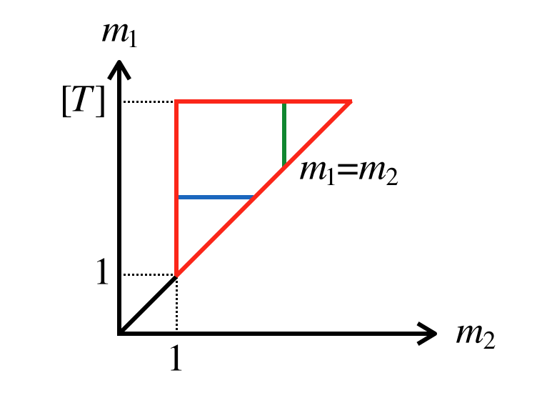
Figure 1: Change of the order of summation.

Thus,

$$S_{1}=\sum_{m_{2}=1}^{[t]}\sum_{m_{1}=m_{2}}^{[t]}\dfrac{1}{\left(m_{1}+m_{2}\right)^{\sigma_{1}+it}}\dfrac{1}{m_{2}^{\sigma_{2}-it}}\dfrac{1}{m_{1}^{\sigma_{3}}},$$

or

$$S_{1}=\sum_{m_{2}=1}^{[t]}\sum_{m_{1}=m_{2}}^{[t]}\dfrac{1}{\left(m_{1}+m_{2}\right)^{\sigma_{1}+it}}\dfrac{1}{m_{2}^{\sigma_{2}+1-it}}\dfrac{m_{2}}{m_{1}^{\sigma_{3}}}.$$ (4.11)

Using partial summation and the fact that $\frac{m_{2}}{m_{1}^{\sigma_{3}}}\leq 1,$ it follows that

$$S_{1}=O\left(|\tilde{S}_{1}|\right),\qquad t\to\infty,$$ (4.12)

where

$$\tilde{S}_{1}=\sum_{m_{2}=1}^{[t]}\sum_{m_{1}=m_{2}}^{[t]}\dfrac{1}{\left(m_{1}+m_{2}\right)^{\sigma_{1}+it}}\dfrac{1}{m_{2}^{\sigma_{2}+1-it}}.$$ (4.13)

Then, proceeding as with the sum $S_{A}$ in (4.3), we obtain the estimate (4.2), i.e.,

$$S_{1}=O\left(t^{\frac{1}{2}-\sigma_{1}}\ln t\right),\qquad t\to\infty.$$ (4.14)

In order to estimate $S_{2}$, we first note that

$$\big{|}S_{2}\big{|}\leq\sum_{m_{1}=1}^{[t]}\Bigg{|}\sum_{m_{2}=m_{1}+1}^{[t]}\dfrac{1}{\left(m_{1}+m_{2}\right)^{\sigma_{1}+it}}\dfrac{1}{m_{2}^{\sigma_{2}-it}}\Bigg{|}\dfrac{1}{m_{1}^{\sigma_{3}}}.$$ (4.15)

Then, taking into consideration that $m_{1}<m_{2}$, we can use the following “crude” estimate for the $m_{2}$ sum:

$$\Bigg{|}\sum_{m_{2}=m_{1}+1}^{[t]}\dfrac{1}{\left(m_{1}+m_{2}\right)^{\sigma_{1}+it}}\dfrac{1}{m_{2}^{\sigma_{2}-it}}\Bigg{|}\leq\int_{m_{1}+1}^{t}\dfrac{1}{\left(m_{1}+x\right)^{\sigma_{1}}}\dfrac{1}{x^{\sigma_{2}}}dx:=J\left(m_{1},t\right).$$ (4.16)

But,

$$m_{1}<x,\ \text{ or }\quad m_{1}+x<2x,\ \text{ or }\quad\left(m_{1}+x\right)^{-\sigma_{1}}<(2x)^{-\sigma_{1}}.$$

Thus,

$$J\left(m_{1},t\right)<\int_{m_{1}+1}^{t}2^{-\sigma_{1}}x^{-\sigma_{1}-\sigma_{2}}dx=O\left(t^{1-\sigma_{1}-\sigma_{2}}\right)+O\left(m_{1}^{1-\sigma_{1}-\sigma_{2}}\right)=O\left(t^{1-\sigma_{1}-\sigma_{2}}\right),\quad t\to\infty,$$

since $\sigma_{1}+\sigma_{2}<1$. Hence, equations (4.15) and (4.16) yield

$$\big{|}S_{2}\big{|}=O\left(t^{1-\sigma_{1}-\sigma_{2}}\int_{1}^{t}\frac{dx}{x^{\sigma_{3}}}\right)=O\left(t^{1-\sigma_{1}-\sigma_{2}}\right)\times\begin{cases}O(\ln t),&\sigma_{3}=1,\\ O(1),&\sigma_{3}>1,\end{cases}\qquad t\to\infty.$$ (4.17)

∎

Remark 4.2.

One can apply the estimate used in (4.17) to $S_{1}$, and then the estimates (4.14) and (4.7) should be substituted by (4.17). Furthermore, for the special cases $\sigma_{1}=\sigma-1,\ \sigma_{2}=\sigma$ and $\sigma_{3}=1$, with $\sigma\in(0,1)$, the estimates (4.2) and (4.7) take the form

$$\big{|}S_{A}\big{|}=O\left(t^{\frac{3}{2}-\sigma}\ln t\right),\qquad t\to\infty,$$ (4.18)

and

$$\big{|}S_{B}\big{|}=\begin{cases}O\left(t^{2-2\sigma}\ln t\right),&0<\sigma<\frac{1}{2},\\ O\left(t^{\frac{3}{2}-\sigma}\ln t\right),&\frac{1}{2}\leq\sigma<1,\end{cases}\qquad t\to\infty,$$ (4.19)

respectively.

5 Double sums for “small” sets of summation

The analysis presented in [F] requires estimating the following sum:

$$\mathop{\sum\sum}_{(m_{1},m_{2})\in M}\frac{1}{m_{1}^{s}(m_{1}+m_{2})^{\bar{s}}},$$ (5.1)

where $M$ is defined by

$$M=\Bigg{\{}m_{1}\in\mathbb{N}^{+},\ m_{2}\in\mathbb{N}^{+}, \quad 1\leq m_{1}\leq[t],\quad 1\leq m_{2}\leq[t],$$

$$\frac{1}{t^{1-\delta_{2}}-1}<\frac{m_{2}}{m_{1}}<t^{1-\delta_{3}}-1,\quad t>0\Bigg{\}},$$ (5.2)

with $\delta_{2}$ and $\delta_{3}$ positive constants.

The above sum can be related to the sum appearing in the first term of the lhs of (3.3) via the following identity:

$$\sum_{m_{1}=1}^{[t]}\sum_{m_{2}=1}^{[t]}\frac{1}{m_{1}^{s}(m_{1}+m_{2})^{\bar{s}}}=\mathop{\sum\sum}_{(m_{1},m_{2})\in M}\frac{1}{m_{1}^{s}(m_{1}+m_{2})^{\bar{s}}}+S_{1}(\sigma,t,\delta_{3})+S_{2}(\sigma,t,\delta_{2}),$$ (5.3)

with

$$S_{1}(\sigma,t,\delta_{3})=\sum_{m_{1}=1}^{\left[\frac{t}{t^{1-\delta_{3}}-1}\right]-1}\sum_{m_{2}=\left[(t^{1-\delta_{3}}-1)m_{1}\right]+1}^{[t]}\frac{1}{m_{1}^{s}(m_{1}+m_{2})^{\bar{s}}}$$ (5.4)

and

$$S_{2}(\sigma,t,\delta_{2})=\sum_{m_{1}=\left[t^{1-\delta_{2}}\right]}^{[t]}\sum_{m_{2}=1}^{\left[\frac{m_{1}}{t^{1-\delta_{2}}-1}\right]-1}\frac{1}{m_{1}^{s}(m_{1}+m_{2})^{\bar{s}}}.$$ (5.5)

Thus, estimating the sum (5.1) requires estimating the sum $S_{1}$ and $S_{2}$. The relevant estimates are presented in Theorems 5.1 and 5.2 below.

By making the change of variables $m_{1}=m$ and $m_{1}+m_{2}=n$ in (5.4) we can rewrite $S_{1}$ in the form

$$S_{1}(\sigma,t,\delta_{3})=\sum_{m=1}^{\left[\frac{t}{t^{1-\delta_{3}}-1}\right]-1}\sum_{n=\left[t^{1-\delta_{3}}m\right]+1}^{[t]+m}\frac{1}{m^{s}n^{\bar{s}}}.$$ (5.6)

Using the equation

$$\frac{t}{t^{1-\delta_{3}}-1}=\frac{t}{t^{1-\delta_{3}}\left(1-t^{\delta_{3}-1}\right)}=t^{\delta_{3}}\left(1+O\left(t^{\delta_{3}-1}\right)\right),\ \ 0<\delta_{3}<1,\qquad t\to\infty,$$

it follows that for $\delta_{3}<1/2$, the upper bound of the expression $\left[\frac{t}{t^{1-\delta_{3}}-1}\right]-1$ is equal either to $\left[t^{\delta_{3}}\right]$ or to $\left[t^{\delta_{3}}\right]-1$. Thus, it is sufficient to consider the following form of $S_{1}$:

$$S_{1}(\sigma,t,\delta_{3})=\sum_{m=1}^{\left[t^{\delta_{3}}\right]}\sum_{n=\left[t^{1-\delta_{3}}m\right]+1}^{[t]+m}\frac{1}{m^{s}n^{\bar{s}}}.$$ (5.7)

Regarding the sum $S_{2}$, by using the fact that

$$\frac{m_{1}}{t^{1-\delta_{2}}-1}=\frac{m_{1}}{t^{1-\delta_{2}}}\left(1+O\left(t^{\delta_{2}-1}\right)\right)=\frac{m_{1}}{t^{1-\delta_{2}}}+O\left(t^{2\delta_{2}-1}\right),\ \ 0<\delta_{2}<1,\qquad t\to\infty,$$

we conclude that $\left[\frac{m_{1}}{t^{1-\delta_{2}}-1}\right]-1$ is equal either to $\left[\frac{m_{1}}{t^{1-\delta_{2}}}\right]-1$ or to $\left[\frac{m_{1}}{t^{1-\delta_{2}}}\right]$, for $\delta_{2}<1/2$.

Thus, it is sufficient to consider the following form of $S_{2}$:

$$S_{2}(\sigma,t,\delta_{2})=\sum_{m_{1}=\left[t^{1-\delta_{2}}\right]}^{[t]}\sum_{m_{2}=1}^{\left[\frac{m_{1}}{t^{1-\delta_{2}}}\right]}\frac{1}{m_{1}^{s}(m_{1}+m_{2})^{\bar{s}}}.$$ (5.8)

Theorem 5.1.

Define the double sum $S_{1}$ by

$$S_{1}(\sigma,t,\delta)=\sum_{m=1}^{\left[t^{\delta}\right]}\sum_{n=\left[t^{1-\delta}m\right]+1}^{[t]+m}\frac{1}{m^{s}n^{\bar{s}}},\ \qquad 0<\delta<1,\quad s=\sigma+it,\quad 0<\sigma<1,\quad t>0.$$ (5.9)

Then,

$$S_{1}(\sigma,t,\delta)=O\left(t^{\frac{1}{2}-\sigma}\tilde{G}(\sigma,t,\delta)\right)+O\left(\frac{t^{(1-\sigma)\delta}}{t^{\sigma}}\right),\qquad 0<\sigma<1,\leavevmode\nobreak\ t\to\infty,$$ (5.10)

where

$$\tilde{G}(\sigma,t,\delta)=O\left(t^{(1-\sigma)\delta}\right)+O\left(t^{\sigma\delta}\right),\qquad 0<\sigma<1,\quad\sigma\neq\frac{1}{2},\quad t\to\infty,$$ (5.11)

and

$$\tilde{G}\left(\frac{1}{2},t,\delta\right)=O\left(t^{\frac{\delta}{2}}\ln{t}\right),\qquad t\to\infty.$$ (5.12)

Proof.

It is convenient to split the $S_{1}$ sum in terms of the following two sums:

$$S_{A}(\sigma,t,\delta)=\sum_{m=1}^{\left[t^{\delta}\right]}\sum_{n=\left[t^{1-\delta}m\right]+1}^{[t]}\frac{1}{m^{s}n^{\bar{s}}},\quad 0<\sigma<1,\quad t>0,$$ (5.13)

and

$$S_{B}(\sigma,t,\delta)=\sum_{m=1}^{\left[t^{\delta}\right]}\sum_{n=[t]+1}^{[t]+m}\frac{1}{m^{s}n^{\bar{s}}},\quad 0<\sigma<1,\quad t>0.$$ (5.14)

Thus, computing $S_{1}$ reduces to computing $S_{A}$ and $S_{B}$:

$$S_{1}(\sigma,t,\delta)=S_{A}(\sigma,t,\delta)+S_{B}(\sigma,t,\delta).$$ (5.15)

We first analyze $S_{B}$. In order to estimate the $n$-sum of $S_{B}$ we employ the identity ((i)) with $\eta=2\pi(t+m)$, equivalently $\left[\frac{\eta}{2\pi}\right]=[t]+m$ :

$$\sum_{n=[t]+1}^{[t]+m}\frac{1}{n^{\bar{s}}}=\frac{1}{1-\bar{s}}\left(t+m\right)^{1-\bar{s}}+O(t^{-\sigma}),\quad 0<\sigma<1,\quad t\to\infty.$$ (5.16)

We note that

$$\frac{1}{1-\bar{s}}\frac{\left(t+m\right)^{1-\bar{s}}}{m^{s}} =\frac{1}{1-\sigma+it}\frac{\left(t+m\right)^{1-\sigma}}{m^{\sigma}}\frac{\left(t+m\right)^{it}}{m^{it}}$$

$$=-\frac{i}{1-\frac{i(1-\sigma)}{t}}t^{-\bar{s}}\left(1+\frac{m}{t}\right)^{1-\sigma}\frac{1}{m^{\sigma}}\left(\frac{1}{t}+\frac{1}{m}\right)^{it}.$$

Using this expression in (5.16) and then substituting the resulting sum in (5.14) we find

$$S_{B}(\sigma,t,\delta)=O(t^{-\sigma})\sum_{m=1}^{\left[t^{\delta}\right]}\frac{1}{m^{s}}+O(t^{-\sigma})\sum_{m=1}^{\left[t^{\delta}\right]}\left\{\left(1+\frac{m}{t}\right)^{1-\sigma}\right.\\ \left.\times\frac{1}{m^{\sigma}}\left(\frac{1}{t}+\frac{1}{m}\right)^{it}\right\},\quad 0<\sigma<1,\quad t\to\infty.$$ (5.17)

Using the fact that the function

$$\left(1+\frac{m}{t}\right)^{1-\sigma},\quad 1\leq m\leq t^{\delta},\quad 0\leq\sigma\leq 1,\quad t>0,$$

is bounded, and employing the classical result on partial summation of single sums, see for example 5.2.1 of [T], it is possible to associate the second sum appearing in (5.17) with

$$\tilde{S}_{B}(\sigma,t,\delta)=\sum_{m=1}^{\left[t^{\delta}\right]}\frac{1}{m^{\sigma}}e^{if(m)},$$ (5.18)

where $f(m)$ is defined in (2.2). Furthermore, recalling that $\tilde{S}_{B}$ can be estimated using (2.17), we obtain

$$\tilde{S}_{B}(\sigma,t,\delta)=O\left(t^{(1-\sigma)\delta}\right),\quad t\to\infty,$$ (5.19)

hence, it follows that

$$\left|\sum_{m=1}^{\left[t^{\delta}\right]}\left(1+\frac{m}{t}\right)^{1-\sigma}\frac{1}{m^{\sigma}}\left(\frac{1}{t}+\frac{1}{m}\right)^{it}\right|=O\left(t^{(1-\sigma)\delta}\right),\qquad t\to\infty.$$

The first sum in (5.17) satisfies an identical estimate with the above, and then equation (5.17) implies

$$S_{B}(\sigma,t,\delta)=O\left(t^{-\sigma+(1-\sigma)\delta}\right),\quad t\to\infty.$$ (5.20)

We next analyze $S_{A}$. For the evaluation of the $n$-sum in the double sum $S_{A}$ defined in (5.13) we will employ the asymptotic formula (2.7) with

$$\frac{t}{\eta_{1}}=t,\quad\text{i.e.},\quad\eta_{1}=1,$$

and

$$\frac{t}{\eta_{2}}+1=t^{1-\delta}m+1,\quad\text{i.e.},\quad\eta_{2}=\frac{t^{\delta}}{m}.$$

If $m=1$ then $\eta_{2}=t^{\delta}$, and if $m=t^{\delta}$ then $\eta_{2}=1$. Thus, the inequalities in (2.7) are satisfied and hence equation (2.7) yields

$$\sum_{n=\left[t^{1-\delta}m\right]+1}^{[t]}\frac{1}{n^{\bar{s}}}=\chi(\bar{s})\sum_{n=1}^{\left[\frac{t^{\delta}}{2\pi m}\right]}\frac{1}{n^{1-\bar{s}}}+\bar{E}\left(\sigma,t,\frac{t^{\delta}}{m}\right)-\bar{E}(\sigma,t,1),\leavevmode\nobreak\ 0<\sigma<1,\leavevmode\nobreak\ t\to\infty.$$ (5.21)

Inserting (5.21) into the definition (5.13) of $S_{A}$ we find

$$S_{A}(\sigma,t,\delta)=\chi(\bar{s})\sum_{m=1}^{\left[t^{\delta}\right]}\sum_{n=1}^{\left[\frac{t^{\delta}}{2\pi m}\right]}\frac{1}{m^{s}}\frac{1}{n^{1-\bar{s}}}+\chi(\bar{s})\sum_{m=1}^{\left[t^{\delta}\right]}\left[\bar{E}\left(\sigma,t,\frac{t^{\delta}}{m}\right)-\bar{E}(\sigma,t,1)\right],\\ \quad 0<\sigma<1,\quad t\to\infty.$$ (5.22)

The occurrence of the term $t^{\delta}$ in the above sums implies that these sums can be easily estimated:

$$\left|\sum_{m=1}^{\left[t^{\delta}\right]}\sum_{n=1}^{\left[\frac{t^{\delta}}{2\pi m}\right]}\frac{1}{m^{s}}\frac{1}{n^{1-\bar{s}}}\right|\leq\int_{1}^{t^{\delta}}\text{d}x\leavevmode\nobreak\ x^{-\sigma}\int_{1}^{\frac{t^{\delta}}{2\pi x}}\text{d}y\leavevmode\nobreak\ y^{\sigma-1}=\tilde{G}(\sigma,t,\delta),\\ 0<\sigma<1,\quad t\to\infty,$$ (5.23)

where

$$\tilde{G}(\sigma,t,\delta)=O\left(t^{(1-\sigma)\delta}\right)+O\left(t^{\sigma\delta}\right),\quad 0<\sigma<1,\quad\sigma\neq\frac{1}{2},\quad t\to\infty,$$

and

$$\tilde{G}\left(\frac{1}{2},t,\delta\right)=O\left(t^{\frac{\delta}{2}}\ln{t}\right),\quad t\to\infty.$$

Recalling the asymptotic formula

$$\chi(s)=\left(\frac{2\pi}{t}\right)^{s-\frac{1}{2}}e^{it}e^{\frac{i\pi}{4}}\left(1+O\left(\frac{1}{t}\right)\right),\quad 0<\sigma<1,\quad t\to\infty,$$ (5.24)

which is derived in the Appendix A of [FL], it follows that

$$S_{A}=O\left(t^{\frac{1}{2}-\sigma}\right)\tilde{G}(\sigma,t,\delta),\quad t\to\infty.$$ (5.25)

Equations (5.15), (5.20) and (5.25) imply (5.10).

∎

For the estimation of $S_{A}$, which gives the dominant contribution of $S_{1}$, one can also use an alternative approach, which is based on classical techniques appearing in [T, T2], and obtain slightly weaker, but essentially similar results. In this connection we obtain the following Lemma:

Lemma 5.1.

Let $S_{A}$ be defined by (5.13). Then

$$S_{A}=O\left(t^{\frac{1}{2}-\sigma}\ln t\right)\tilde{G}(\sigma,t,\delta),\qquad 0<\sigma<1,\leavevmode\nobreak\ t\to\infty.$$ (5.26)

Proof.

Observing that $m$ takes relatively “small” values in the set of summation of $S_{A}$, we use the following inequality without losing crucial information

$$\left|S_{A}\right|<\sum_{m=1}^{\left[t^{\delta}\right]}\frac{1}{m^{\sigma}}\left|\sum_{n=\left[t^{1-\delta}m\right]+1}^{[t]}\frac{1}{n^{\bar{s}}}\right|.$$

Then, we estimate the $n$-sum using Theorem 5.9 of [T], namely

$$\sum_{a<n\leq b\leq 2a}n^{it}=O\left(t^{\frac{1}{2}}\right)+O\left(at^{-\frac{1}{2}}\right).$$

Using partial summation and the fact that $a>mt^{1-\delta}$, similarly to the proof of Theorem 5.12 of [T], we obtain that

$$\sum_{n=\left[t^{1-\delta}m\right]+1}^{[t]}\frac{1}{n^{\bar{s}}}=O\left(t^{\frac{1}{2}}t^{-(1-\delta)\sigma}m^{-\sigma}\ln t\right),\qquad t\to\infty.$$

Thus,

$$S_{A}=\sum_{m=1}^{\left[t^{\delta}\right]}\frac{1}{m^{2\sigma}}O\left(t^{\frac{1}{2}-\sigma}t^{\delta\sigma}\ln t\right),\qquad t\to\infty.$$ (5.27)

Applying in (5.27) the fact that

$$\sum_{m=1}^{\left[t^{\delta}\right]}\frac{1}{m^{2\sigma}}=\begin{cases}O\left(t^{(1-2\sigma)\delta}\right),&0<\sigma<\frac{1}{2},\\ O(\ln t),&\sigma=\frac{1}{2},\\ O(1),&\frac{1}{2}<\sigma<1,\end{cases}$$

yields (5.26). ∎

Remark 5.1.

The estimates of $S_{A}$ given in (5.25) and (5.26) differ only by a $\ln t$ term. The approach in the proof of Lemma 5.1 implies that for $0<\delta<1/3,$ the estimate of $S_{A}$ is essentially the best which one should expect via the classical techniques presented in [T, T2, K]. In particular, for $\sigma=1/2$, these techniques together with Theorem 5.14 of [T], suggest the estimate

$$S_{A}\left(\frac{1}{2},t,\delta\right)=\begin{cases}O\left(t^{\frac{\delta}{2}}(\ln t)^{2}\right),&0<\delta<\frac{1}{3},\\ O\left(t^{\frac{1}{6}}(\ln t)^{2}\right),&\frac{1}{3}\leq\delta<1,\end{cases}\qquad t\to\infty.$$

Theorem 1 of [T2] together with the Theorem 2.16 of [K], does not appear to give an essential improvement of the above estimate.

Theorem 5.2.

Define the double sum $S_{2}(\sigma,t,\delta)$ by

$$S_{2}(\sigma,t,\delta)=\sum_{m_{1}=\left[t^{1-\delta}\right]}^{[t]}\sum_{m_{2}=1}^{\left[\frac{m_{1}}{t^{1-\delta}}\right]}\frac{1}{m_{1}^{s}(m_{1}+m_{2})^{\bar{s}}},\quad 0<\delta<1,\ s=\sigma+it,\leavevmode\nobreak\ 0<\sigma<1,\leavevmode\nobreak\ t>0.$$ (5.28)

Then,

$$S_{2}(\sigma,t,\delta)=O\left(t^{1-2\sigma+(2\sigma+1)\delta}\right),\quad 0<\sigma<1,\quad t\to\infty.$$ (5.29)

Proof.

We find more convenient to treat this sum using some of the ‘crude’ methods, involving the integration, in order to benefit from the smallness of the set of summation. Indeed, we observe that

$$\left|S_{2}\right|\leq\int_{t^{1-\delta}}^{t}\int_{1}^{\frac{x}{t^{1-\delta}}}\frac{1}{x^{\sigma}(x+y)^{\sigma}}dydx:=J_{2}(t).$$ (5.30)

Using the fact that $t>x>t^{1-\delta}$, as well as that $x+y>t^{1-\delta}$, then

$$J_{2}(t) <\frac{1}{t^{2\sigma(1-\delta)}}\int_{t^{1-\delta}}^{t}\int_{1}^{\frac{x}{t^{1-\delta}}}dydx<\frac{1}{t^{2\sigma(1-\delta)}}\int_{t^{1-\delta}}^{t}\int_{1}^{t^{\delta}}dydx$$

$$=\frac{1}{t^{2\sigma(1-\delta)}}\left(t-t^{1-\delta}\right)\left(t^{\delta}-1\right)=O\left(t^{1-2\sigma+(2\sigma+1)\delta}\right).$$

∎

Remark 5.2.

Using the techniques developed in [T2] and [K] as are appropriately modified in Appendix B, we obtain the slightly better estimate

$$S_{2}(\sigma,t,\delta)=O\left(t^{1-2\sigma}t^{2\delta\sigma}(\ln{t})^{3}\right),\quad 0<\sigma<1,\quad t\to\infty.$$ (5.31)

The fact that this result does not provide a significant improvement to (5.29) is due to the fact that in the latter approach we have exploited the smallness of the set of summation via the integration process.

It is possible to improve further the estimate (5.29), by obtaining a more accurate estimate of the integral $J_{2}(t)$. Indeed, applying the following Lemma to (5.30), we obtain

$$S_{2}=O\left(t^{1-2\sigma+\delta}\right),\qquad 0<\sigma<1,\quad t\to\infty.$$ (5.32)

Lemma 5.2.

Let $J_{2}(t)$ be defined by (5.30). Then,

$$J_{2}(t)=\dfrac{t^{1-2\sigma+\delta}}{2(1-\sigma)}\left(1+O\left(t^{-2\delta(1-\sigma)},t^{-\delta}\right)\right),\quad 0<\sigma<1,\quad t\to\infty.$$ (5.33)

Proof.

$$J_{2}(t) =\int_{t^{1-\delta}}^{t}\int_{1}^{\frac{x}{t^{1-\delta}}}\frac{1}{x^{\sigma}(x+y)^{\sigma}}dydx=\int_{t^{1-\delta}}^{t}\frac{1}{x^{\sigma}}\left[x^{1-\sigma}\frac{\left(1+t^{\delta-1}\right)^{1-\sigma}}{1-\sigma}-\frac{(x+1)^{1-\sigma}}{1-\sigma}\right]dx$$

$$=\frac{1}{1-\sigma}\int_{t^{1-\delta}}^{t}x^{1-2\sigma}\left[\left(1+t^{\delta-1}\right)^{1-\sigma}-\left(1+\frac{1}{x}\right)^{1-\sigma}\right]dx$$

$$=\frac{1}{1-\sigma}\int_{t^{1-\delta}}^{t}x^{1-2\sigma}\left[1+(1-\sigma)t^{\delta-1}-1-\frac{1-\sigma}{x}+O\left(t^{2(\delta-1)},\frac{1}{x^{2}}\right)\right]dx,\quad t\to\infty.$$

Using the fact that $x>t^{1-\delta}$, the above integral takes the form

$$J_{2}(t) =t^{\delta-1}\int_{t^{1-\delta}}^{t}x^{1-2\sigma}dx-\int_{t^{1-\delta}}^{t}x^{-2\sigma}dx+\int_{t^{1-\delta}}^{t}x^{1-2\sigma}dx\ O\left(t^{2(\delta-1)}\right),\quad t\to\infty,$$

which yields (5.33). ∎

Theorem 5.3.

Let $\delta\in\left(0,\frac{1}{2}\right)$ and the double sum $S_{2}(\sigma,t,\delta)$ be defined by (5.28). Then,

$$S_{2}(\sigma,t,\delta)=\begin{cases}O\left(t^{1-2\sigma}\right)+O\left(t^{\delta-2\sigma}\right),\quad&0<\sigma<\frac{1}{2},\\ O\left(\ln t\right)+O\left(t^{\delta-1}\right),\quad&\sigma=\frac{1}{2},\end{cases}\quad t\to\infty.$$ (5.34)

Proof.

Letting $m_{1}=m$ and $m_{1}+m_{2}=n$ in the definition (5.28) of $S_{2}$ we find

$$S_{2}(\sigma,t,\delta)=\sum_{m=\left[t^{1-\delta}\right]}^{[t]}\sum_{n=1+m}^{\left[m\left(1+t^{\delta-1}\right)\right]}\frac{1}{m^{s}n^{\bar{s}}}.$$ (5.35)

It is convenient to split the $S_{2}$ sum in terms of the following two sums:

$$S_{A}(\sigma,t,\delta)=\sum_{m=\left[t^{1-\delta}\right]}^{[t]}\sum_{n=1+m}^{P(t)}\frac{1}{m^{s}n^{\bar{s}}},\quad 0<\sigma<1,\quad t>0,$$ (5.36)

and

$$S_{B}(\sigma,t,\delta)=\sum_{m=\left[t^{1-\delta}\right]}^{[t]}\sum_{n=[t]+1}^{\left[m\left(1+t^{\delta-1}\right)\right]}\frac{1}{m^{s}n^{\bar{s}}},\quad 0<\sigma<1,\quad t>0,$$ (5.37)

where $P(t)=\min\left\{[t],\left[m\left(1+t^{\delta-1}\right)\right]\right\}$.

Hence

$$S_{2}(\sigma,t,\delta)=S_{A}(\sigma,t,\delta)+S_{B}(\sigma,t,\delta),\quad 0<\sigma<1,\quad t>0.$$ (5.38)

We first analyze $S_{B}$. In this connection we define the function $l(t)$ by

$$l(t)=\left[t-t^{\delta}\right]+1,\quad t>0.$$ (5.39)

We observe that the upper limit of the $n$-sum of $S_{B}$ is greater or equal to $[t]+1$ only if $m\geq l(t)$. Thus, we rewrite $S_{B}$ in the form

$$S_{B}(\sigma,t,\delta)=\sum_{m=l(t)}^{[t]}\sum_{n=[t]+1}^{\left[m\left(1+t^{\delta-1}\right)\right]}\frac{1}{m^{s}n^{\bar{s}}},\quad 0<\sigma<1,\quad t>0.$$ (5.40)

In order to estimate the $n$-sum of $S_{B}$ we employ the identity ((i)) with $\eta=2\pi m\left(1+t^{\delta-1}\right)$:

$$\sum_{n=[t]+1}^{\left[m\left(1+t^{\delta-1}\right)\right]}\frac{1}{n^{\bar{s}}}=\frac{1}{1-\bar{s}}\left(1+t^{\delta-1}\right)^{1-\bar{s}}m^{1-\bar{s}}+O(t^{-\sigma}),\qquad 0<\sigma<1,\quad t\to\infty.$$ (5.41)

$$S_{B}(\sigma,t,\delta)=-\frac{i}{t}\sum_{m=l(t)}^{[t]} \frac{m^{1-2\sigma}}{1-\frac{i(1-\sigma)}{t}}\left(1+t^{\delta-1}\right)^{1-\bar{s}}$$

$$+O(t^{-\sigma})\sum_{m=l(t)}^{[t]}m^{-s},\qquad 0<\sigma<1,\quad t\to\infty.$$ (5.42)

Proceeding as with the evaluation of $S_{B}$ in Theorem 5.1 we find that

$$\left|\sum_{m=l(t)}^{[t]}m^{-s}\right|\leq\frac{1}{1-\sigma}\left[t^{1-\sigma}-\left(t-t^{\delta}+1\right)^{1-\sigma}\right]=O\left(\frac{t^{\delta}}{t^{\sigma}}\right),\quad 0<\sigma<1,\quad t\to\infty.$$

Similarly, the first sum of (5) is of order $t^{\delta}/t^{2\sigma}$. Thus,

$$S_{B}(\sigma,t,\delta)=O\left(\frac{t^{\delta}}{t^{2\sigma}}\right),\quad 0<\sigma<1,\quad t\to\infty.$$ (5.43)

We next consider $S_{A}$. Our approach is based on the application of the asymptotic formula (2.7) in the inner sum of $S_{A}$.

Indeed, for the case that $P(t)=[m\left(1+t^{\delta-1}\right)]$, by applying (2.7) in the inner sum of $S_{A}$ with $\frac{t}{\eta_{2}}=m$ and $\frac{t}{\eta_{1}}=m\left(1+t^{\delta-1}\right)$, we obtain

$$\eta_{2}=\frac{t}{m}\qquad\text{and}\qquad\eta_{1}=\frac{t}{m\left(1+t^{\delta-1}\right)}=\frac{t}{m}-\frac{t^{\delta}}{m}.$$

Observing that $\frac{t^{\delta}}{m}\leq\frac{t^{\delta}}{t^{1-\delta}}=t^{2\delta-1}=o(1),$ and using that dist$\left(\frac{\eta_{j}}{2\pi},\mathbb{Z}\right)>\epsilon,\quad j=1,2,$ we obtain that $\left[\frac{\eta_{1}}{2\pi}\right]=\left[\frac{\eta_{2}}{2\pi}\right]$.

Similarly, for the case $P(t)=[t]$ we obtain $\left[\frac{\eta_{1}}{2\pi}\right]=\left[\frac{\eta_{2}}{2\pi}\right]=0$.

Thus, for the inner sum of $S_{A}$ the set of the summation of the rhs of (2.7) is empty. Furthermore, the definition of $E(\sigma,t,\eta)$ given in (2.8a) implies that

$$E(\sigma,t,\eta_{j})=O\left(\left(\frac{\eta_{j}}{t}\right)^{\sigma}\right)=O\left(\frac{1}{m^{\sigma}}\right),\qquad j=1,2.$$

Thus,

$$S_{A}(\sigma,t,\delta)=O\left(\sum_{m=\left[t^{1-\delta}\right]}^{[t]}\frac{1}{m^{2\sigma}}\right),$$ (5.44)

which along with (5.43) yields the estimate (5.34).

∎

Remark 5.3.

For the particular case $\sigma=1/2$ the estimates of $S_{2}$ given by (5.29), (5.31) and (5.32), take the form $O\left(t^{\frac{3}{2}\delta}\right),\ O\left(t^{\delta}(\ln t)^{3}\right)$ and $O\left(t^{\delta}\right)$, respectively, which for $\delta>0$ arbitrarily small, are essentially the same.

We note that even the extensive use of the techniques appearing in Appendix B does not appear to provide an estimate better than $O\left(t^{\delta}\right)$, which is essentially the same with the estimate obtained via the “rough” techniques of Lemma 5.2, for $\delta\in(0,1)$.

The result of Theorem 5.3 yields the estimate $O(\ln t)$, for $\delta\in\left(0,\frac{1}{2}\right)$, which provides a significant improvement of the classical techniques on the estimate of $S_{2}$, when $\delta$ is not arbitrarily small. In [F], the sum $S_{2}$ is estimated via a completely different approach, and this yields the estimate $O\left(t^{\delta-\frac{1}{2}}\ln t\right)+O(1)$, for $\delta\in(0,1)$.

Appendix A (proof of (4.5))

Let $\chi(s)$ be defined by (2.8e), then it is shown in [FL] that

$$\chi(s)=\left(\frac{2\pi}{t}\right)^{s-\frac{1}{2}}e^{it}e^{i\frac{\pi}{4}}\left[1+O\left(\frac{1}{t}\right)\right],\qquad s=\sigma+it,\quad\sigma\in\mathbb{R},\quad t\to\infty.$$ (A.1)

Employing the well known identity

$$\zeta(s)=\chi(s)\zeta(1-s),\qquad s\in\mathbb{C},$$ (A.2)

with $s=\sigma-1+it,$ we find

$$\zeta(\sigma-1+it)=\chi(\sigma-1+it)\zeta(2-\sigma-it).$$ (A.3)

Suppose that $0<\sigma<1$. Using the fact that $\zeta(2-\sigma-it)$ is bounded as $t\to\infty$, as well as the asymptotic estimate (A.1), equation (A.3) implies that

$$\zeta(\sigma-1+it)=O\left(t^{\frac{3}{2}-\sigma}\right),\qquad 0<\sigma<1,\quad t\to\infty.$$ (A.4)

Applying equation (3.1) of Theorem 3.1 in [FL], for $\eta=2\pi t$ we derive the following result:

$$\zeta(s)= \sum_{n=1}^{[t]}n^{-s}-\frac{1}{1-s}t^{1-s}$$ (A.5)

$$+\frac{e^{-\frac{i\pi(1-s)}{2}}}{(2\pi)^{1-s}}\sum_{n=1}^{\infty}\sum_{j=0}^{N-1}e^{-nz-it\ln{z}}\left(\frac{1}{n+\frac{it}{z}}\frac{d}{dz}\right)^{j}\frac{z^{-\sigma}}{n+\frac{it}{z}}\biggr{|}_{z=i2\pi t}$$

$$+\frac{e^{\frac{i\pi(1-s)}{2}}}{(2\pi)^{1-s}}\sum_{n=2}^{\infty}\sum_{j=0}^{N-1}e^{-nz-it\ln{z}}\left(\frac{1}{n+\frac{it}{z}}\frac{d}{dz}\right)^{j}\frac{z^{-\sigma}}{n+\frac{it}{z}}\biggr{|}_{z=-i2\pi t}$$

$$+O\biggl{(}(2N+1)!!N2^{2N}t^{-\sigma-N}\biggr{)},\qquad 0\leq\sigma\leq 1,\quad N\geq 2,\quad t\to\infty,$$

where the error term is uniform for all $\sigma,N$ in the above ranges and the coefficients $c_{k}(\sigma)$ are given therein. This equation is derived in [FL] under the assumption that $0<\sigma<1$. However, it is straightforward to verify that it is also valid for $-1<\sigma<0.$ Equations (A.5) and (A.4) imply that

$$\sum_{m=1}^{[t]}\dfrac{1}{m^{\sigma-1+it}}=O\left(t^{\frac{3}{2}-\sigma}\right),\qquad 0<\sigma<1,\quad t\to\infty.$$ (A.6)

Appendix B (proof of (5.31))

Letting $m_{1}=m$ and $m_{1}+m_{2}=n$ in the definition (5.28) of $S_{2}$ we find

$$S_{2}(\sigma,t,\delta)=S_{A}(\sigma,t,\delta)+S_{B}(\sigma,t,\delta),\quad 0<\sigma<1,\quad t>0,$$ (B.1)

with $S_{A}$ and $S_{B}$ defined in (5.36) and (5.37), respectively.

The analysis in Theorem 5.3 yields

$$S_{B}(\sigma,t,\delta)=O\left(\frac{t^{\delta}}{t^{2\sigma}}\right),\quad 0<\sigma<1,\quad t\to\infty.$$ (B.2)

We next consider $S_{A}$. The derivation of this estimate consists of two parts:

• The first part involves the proof

  $$\sum_{m=\left[t^{1-\delta}\right]}^{[t]}\sum_{n=m+1}^{[t]}\frac{1}{m^{it}n^{-it}}=O\left(t(\ln{t})^{3}\right),\quad t\to\infty.$$ (B.3)

• The second part involves the partial summation technique for double sums.

For the first part we first prove that

$$\sum_{m=M}^{M^{\prime}}\sum_{n=N}^{N^{\prime}}\dfrac{1}{m^{it}}\dfrac{1}{n^{-it}}=O(t\ln t),$$ (B.4)

with $n>m$, and

$$\begin{cases}A_{1}\sqrt{t}<M<M^{\prime}<2M<A_{3}t,\\ A_{2}\sqrt{t}<N<N^{\prime}<2N<A_{4}t,\end{cases}$$

for some positive constants $\{A_{j}\}_{1}^{4}$.

In this connection, we divide the set of summation similarly to the division implemented in Theorem 1 of [T2], namely, in “small” rectangles $\Delta_{p,q}$, such that

$$\begin{cases}M+p\l_{1}\leq m\leq M+p\l_{1}+\l_{1},\\ N+q\l_{2}\leq n\leq N+q\l_{2}+\l_{2}.\end{cases}$$

Moreover, we pick

$$\begin{cases}\l_{1}=c_{1}\frac{M^{2}}{t},\\ \l_{2}=c_{2}\frac{N^{2}}{t},\end{cases}$$ (B.5)

for some positive constants $c_{1}$ and $c_{2}$.

We make the following observations:

• $\displaystyle\begin{cases}1\leq\l_{1}\leq M\Leftrightarrow A_{1}\sqrt{t}<M<A_{3}t,\\ 1\leq\l_{2}\leq N\Leftrightarrow A_{2}\sqrt{t}<N<A_{4}t,\end{cases}$ for some positive constants $\{A_{j}\}_{1}^{4}$.

• The number of the “small” rectangles $\Delta_{p,q}$ is $O\left(\dfrac{MN}{\l_{1}\l_{2}}\right)$.

We use Theorem 2.16 of [K] with

$$f(x,y)=t(\ln x-\ln y).$$

Then, in each rectangle $\Delta_{p,q}$, with $n>m$ (equivalently $x>y$), the conditions of this theorem are satisfied with $\lambda_{1}=\frac{t}{M^{2}}$ and $\lambda_{2}=\frac{t}{N^{2}}$, because

$$\big{|}f_{xx}\big{|}=\frac{t}{x^{2}},\quad\big{|}f_{yy}\big{|}=\frac{t}{y^{2}}\quad\text{ and }\ \big{|}f_{xy}\big{|}=0.$$

Using the following facts:

• the conditions $\displaystyle\begin{cases}M>A_{1}\sqrt{t},\\ N>A_{2}\sqrt{t},\end{cases}$ imply that $\displaystyle\begin{cases}\lambda_{1}<\frac{1}{A_{1}^{2}},\\ \lambda_{2}<\frac{1}{A_{2}^{2}}\end{cases}$,

• all the quantities $\ln\big{|}\Delta_{p,q}\big{|},\ \big{|}\ln\lambda_{1}\big{|}$ and $\big{|}\ln\lambda_{2}\big{|}$ are of order $O(\ln t)$,

and employing equation (2.56) of [K], we find

$$\mathop{\sum\sum}_{(m,n)\in\Delta_{p,q}}e^{if(m,n)}=O\left(\dfrac{\ln t}{\frac{t}{MN}}\right).$$ (B.6)

Thus, the fact that the number of the rectangles $\Delta_{p,q}$ is $O\left(\dfrac{MN}{\l_{1}\l_{2}}\right)$, implies that

$$\sum_{m=M}^{M^{\prime}}\sum_{n=N}^{N^{\prime}}e^{if(m,n)}=O\left(\dfrac{MN}{t}\ln t\dfrac{MN}{\l_{1}\l_{2}}\right).$$ (B.7)

Equation (B.4) follows from applying (B.5) in (B.7).

Finally, using the classical splitting for the sets of summation for exponential sums, see [T] and [T2], equation (B.3) follows from applying (B.4) for $O\left(\left(\ln t^{\delta}\right)^{2}\right)=O\left(\left(\delta\ln t\right)^{2}\right)=O\left((\ln t)^{2}\right)$ times.

Considering the second part, under the condition that the expressions

$$b_{m,n}-b_{m+1,n},\quad b_{m,n}-b_{m,n+1},\quad b_{m,n}-b_{m+1,n}-b_{m,n+1}+b_{m+1,n+1},$$ (B.8)

keep their sign, the following result is derived in [T2]:

$$\left|\sum_{m=1}^{M}\sum_{n=1}^{N}a_{m,n}b_{m,n}\right|\leq 5GH,$$ (B.9)

where

$$S_{m,n}\Doteq\sum_{\mu=1}^{m}\sum_{\nu=1}^{n}a_{\mu,\nu},\quad|S_{m,n}|\leq G,\quad 1\leq m\leq M,\quad 1\leq n\leq N,$$ (B.10)

with

$$b_{m,n}\in\mathbb{R},\quad 0\leq b_{m,n}\leq H.$$ (B.11)

We apply the above argument for $\displaystyle b_{m,n}=\frac{1}{m^{\sigma}n^{\sigma}}$, thus the expressions in (B.8) keep their sign, and furthermore

$$H=\dfrac{1}{t^{(1-\delta)\sigma}}\dfrac{1}{t^{(1-\delta)\sigma}}=t^{-2\sigma}t^{2\delta\sigma}.$$

Combining the above result with (B.3) yields

$$S_{A}(\sigma,t,\delta)=O\left(t^{1-2\sigma}t^{2\delta\sigma}(\ln{t})^{3}\right),\quad 0<\sigma<1,\quad t\to\infty.$$ (B.12)

Equations (B.1), (B.2), (B.12) imply (5.31).