Structural Break Detection in High-Dimensional Non-Stationary VAR models

Abolfazl Safikhani and Ali Shojaie

Columbia University and University of Washington

Abstract Assuming stationarity is unrealistic in many time series applications. A more realistic alternative is to allow for piecewise stationarity, where the model is allowed to change at given time points. In this article, the problem of detecting the change points in a high-dimensional piecewise vector autoregressive model (VAR) is considered. Reformulated the problem as a high-dimensional variable selection, a penalized least square estimation using total variation LASSO penalty is proposed for estimation of model parameters. It is shown that the developed method over-estimates the number of change points. A backward selection criterion is thus proposed in conjunction with the penalized least square estimator to tackle this issue. We prove that the proposed two-stage procedure consistently detects the number of change points and their locations. A block coordinate descent algorithm is developed for efficient computation of model parameters. The performance of the method is illustrated using several simulation scenarios.

Keywords: High-dimensional time series; Structural break; LASSO; Piecewise stationary.

1 Introduction

Emerging applications in biology (Michailidis & d’Alché Buc, 2013; Smith, 2012; Fujita et al., 2007; Mukhopadhyay & Chatterjee, 2006) and finance (De Mol et al., 2008; Fan et al., 2011) have sparked an interest in methods for analyzing high-dimensional time series. Recent work includes new regularized estimation procedures for vector autoregressive (VAR) models (Basu & Michailidis, 2015; Nicholson et al., 2017), high-dimensional generalized linear models (Hall et al., 2016) and high-dimensional point processes (Hansen et al., 2015; Chen et al., 2017). These methods generalize the earlier work on methods for high-dimensional longitudinal data (Shojaie & Michailidis, 2010; Shojaie et al., 2012), and handle the theoretical challenges of resulting from the temporal dependence among observations. Related methods have also focused on joint estimation of multiple time series (Qiu et al., 2016), estimation of (inverse) covariance matrices (Xiao & Wu, 2012; Chen et al., 2013; Tank et al., 2015), and estimation of high-dimensional systems of differential equations (Lu et al., 2011; Chen et al., 2016).

Despite considerable progress, both on computational and theoretical fronts, the vast majority of existing work on high-dimensional time series assumes that the underlying process is stationary. However, multivariate time series observed in many modern applications are nonstationary. For instance, Clarida et al., (2000) show that the effect of inflation on interest rates varies across Federal Reserve regimes. Similarly, as pointed out by Ombao et al., (2005), electroencephalograms (EEGs) recorded during an epileptic seizure display amplitudes and spectral distribution that vary over time. This nonstationarity is illustrated in Figure 1, which shows the EEG signals recorded at 18 EEG channels during an epileptic seizure from a patient diagnosed with left temporal lobe epilepsy (Ombao et al., 2005). The sampling rate in this data is 100 Hz and the total number of time points per EEG is $T=32,768$ over $\sim 238$ seconds. Based on the neurologist’s estimate, the seizure took place at $t=185~{}s$. The plot of the EEGs also suggests that the magnitude and the variability of these signals change simultaneously around that time. Assuming stationarity when analyzing such high-dimensional times series can severely bias estimation and inference procedures.

Figure 1: EEG signals from a patient diagnosed with left temporal lobe epilepsy. The data was recorded at 18 locations on the scalp during an epileptic seizure over 32,768 time points.

Non-stationary VAR models have been primarily studied in univariate or low-dimensional settings. Existing approaches include models that fully parameterize the evolution of the transition matrices of time-varying VARs, or enforce a Bayesian prior on the structure of the time-dependence (Primiceri, 2005). An alternative approach is to assume that the VAR process is locally stationary; locally stationarity means that, in each small time interval, the process is well-approximated by a stationary one. This notion has been studied in low-dimensions by Dahlhaus, (2012); Sato et al., (2007) proposed a wavelet-based method for estimating the time-varying coefficients of the VAR model.

Recently, Ding et al., (2016) considered estimation of high-dimensional time-varying VARs by solving time-varying Yule-Walker equations based on kernelized estimates of variance and auto-covariance matrices. This approach is a significant step forward, and facilitates estimation of nonstationary VAR models in high dimensions. However, local stationarity may not be a suitable assumption in many applications. For instance, when analyzing EEG data from patients who suffer from epileptic seizure, it is expected that interactions among brain regions change before and after the occurrence of seizure. Assuming that the process can be locally approximated by a stationary one at the time of seizure may be unrealistic. A more natural assumption in such settings is that the process is piecewise stationary — that the process is stationary in each of (potentially many) regions, e.g., before and after seizure.

Existing methods for analyzing piecewise stationary time series have primarily focused on univariate time series. For instance, Davis et al., (2006), Chan et al., (2014) and Bai, (1997) propose different approaches for identifying structural breakpoints at which the behavior of a univariate time series changes. By identifying structural breaks in mean and/or covariance structures over time, these approaches provide more flexible than those assuming stationarity. However, their extension to multivariate and high-dimensional VARs have not been explored. The only exception is the SLEX method of Ombao et al., (2005), who analyzed the data from Figure 1 and identified break points associated with seizure using a wavelet-based approach. However, to deal with the large number of time series, Ombao et al., (2005) apply a dimension reduction step. Thus, their method does not reveal mechanisms of interactions among brain regions, which is a key interest in understanding changes in brain function before, during and after seizure. In this paper we bridge this gap by developing a regularized estimation procedure for high-dimensional piecewise stationary VARs with possibly many break points. The proposed approach first identifies the number of break points. It then determines the location of the break points and provides consistent estimates of model parameters. Simulated and real data examples are used to support the theoretical findings of the paper, and illustrate the flexibility of the proposed approach in applications.

The rest of this paper is organized as follows. In Section 2, we describe the piecewise stationary model and the key assumptions. We also present our estimation framework for detecting structural breaks in piecewise stationary VARs. The asymptotic properties of the proposed method are discussed in Section 3. In particular, we show that under reasonable assumptions the structural breaks in high-dimensional VAR models are consistency estimated. To this end, we first establishing the prediction consistency of the proposed method in Section 3.2. Results of simulation experiments are presented in Sections4. In Section 5 we illustrate the utility of the proposed method by applying it to identify structural break points in two multivariate time series. We conclude the paper with a discussion in Section 6. Technical lemmas and proofs are collected in the Appendix.

2 Model and Method

A piecewise stationary VAR model can be viewed as a collection of separate VAR models concatenated at multiple break points over the time period of the observed time series. More specifically, suppose there exist $m_{0}$ break points $0=t_{0}<t_{1}<\cdots<t_{m_{0}}<t_{m_{0}+1}=T+1$ such that

$$y_{t}=\sum_{i=1}^{d}\Phi^{(i,j)}y_{t-i}+\varepsilon_{t},\hskip 56.9055ptt_{j-1}\leq t<t_{j},\hskip 28.45274ptj=1,2,...,m_{0}+1,$$ (1)

where $y_{t}$ is a $p\times 1$ vector of observed time series at time $t$, $\Phi^{(i,j)}$’s are $p\times p$ spares coefficient matrices of the VAR process, $\varepsilon_{t}$ is a multivariate Gaussian white noise with covariance matrix $\Sigma_{\varepsilon}$.

Our goal is to detect the break points $t_{j}$’s together with estimates of the coefficient parameters $\Phi^{(i,j)}$’s in the high-dimensional case where $p\gg T$. To this end, we adopt the idea of change-point detection in Harchaoui & Lévy-Leduc, (2010) and Chan et al., (2014), and extend it to the multivariate, high-dimensional setting. Specifically, our estimation procedure utilizes the following linear regression representation of the VAR process

$$\begin{pmatrix}y_{d}^{\prime}\\ y_{d+1}^{\prime}\\ \vdots\\ y_{T}^{\prime}\end{pmatrix}=\begin{pmatrix}y_{d-1}^{\prime}&\ldots&y_{0}^{\prime}&&0&&\ldots&&0&\\ y_{d}^{\prime}&\ldots&y_{1}^{\prime}&y_{d}^{\prime}&\ldots&y_{1}^{\prime}&&&0&\\ &\vdots&&&&&\ddots&&\\ y_{T-1}^{\prime}&\ldots&y_{T-d}^{\prime}&y_{T-1}^{\prime}&\ldots&y_{T-d}^{\prime}&\ldots&y_{T-1}^{\prime}&\ldots&y_{T-d}^{\prime}\end{pmatrix}\begin{pmatrix}\theta_{1}^{\prime}\\ \theta_{2}^{\prime}\\ \vdots\\ \theta_{n}^{\prime}\end{pmatrix}+\begin{pmatrix}\varepsilon_{d}^{\prime}\\ \varepsilon_{d+1}^{\prime}\\ \vdots\\ \varepsilon_{T}^{\prime}\end{pmatrix},$$ (2)

where $n=T-d+1$, $\Phi^{(.,j)}=\begin{pmatrix}\Phi^{(1,j)}&\ldots&\Phi^{(d,j)}\end{pmatrix}\in\mathbb{R}^{p\times pd}$, $\theta_{1}=\Phi^{(.,1)}$ and

$$\theta_{i}=\left\{\begin{array}[]{ll}\Phi^{(.,i+1)}-\Phi^{(.,i)},&\mbox{when }i=t_{j}\,\,\mbox{for some}\,j\\ 0,&\mbox{otherwise},\end{array}\right.$$ (3)

for $i=2,3,...,n$.

Equation 2 can be written in a compact form as

$$\mathcal{Y}=\mathcal{X}\theta(n)+\varepsilon(n),$$

or, in a vector form, as

$$Y=Z\Theta+E,$$

where $Y=\mbox{vec}(\mathcal{Y})$, $Z=I_{p}\otimes\mathcal{X}$, and $E=\mbox{vec}(\varepsilon(n))$. Denoting $q=np^{2}d$, $Y\in\mathbb{R}^{np\times 1}$, $Z\in\mathbb{R}^{np\times q}$, $\Theta\in\mathbb{R}^{q\times 1}$, and $E\in\mathbb{R}^{np\times 1}$. Note that in this parameterization, $\widehat{\theta}_{i}\neq 0$, $i\geq 2$ implies a change in the VAR coefficients. Therefore, the structural break points $t_{j},j=1,\ldots,m_{0}$ can be estimated as time points $i\geq 2$, where $\widehat{\theta}_{i}\neq 0$. To this end, the first step of our procedure consists of estimating the parameters $\Theta$ using an $\ell_{1}$ penalized least squares regression. Formally,

$$\widehat{\Theta}=\mbox{argmin}_{\Theta}\frac{1}{n}\|Y-Z\Theta\|_{2}^{2}+\lambda_{n}\sum_{i=1}^{n}\|\theta_{i}\|_{1}.$$ (4)

The optimization problem in (4) is convex and can be efficiently solved using a block coordinate descent algorithm (Tseng & Yun, 2009). This algorithm involves updating one of the $\theta_{i}$’s at each iteration, until convergence. The KKT conditions of problem (4), presented in Lemma 2 of Appendix A show that for fixed $i=1,2,\ldots,n$, each update of $\theta_{i}$ at iteration $h+1$ can be calculated as

$$\theta_{i}^{\prime}(h+1)={\left(\sum_{l=i}^{n}Y_{l-1}Y_{l-1}^{\prime}\right)}^{-1}S\left(\sum_{l=i}^{n}Y_{l-1}y_{l}-\sum_{j\neq i}\left(\sum_{l=\max(i,j)}^{n}Y_{l-1}Y_{l-1}^{\prime}\right)\theta_{j}^{\prime}(h);\lambda\right).$$ (5)

Here, $S(.;\lambda)$ is the element-wise soft-thresholding function on all the components of the input matrix, which maps its input $x$ to $x-\lambda$ when $x>\lambda$, $x+\lambda$ when $x<-\lambda$, and $0$ when $|x|\leq\lambda$. The iteration stops when $\|\theta(h+1)-\theta(h)\|_{\infty}<\mbox{tolerance}$; we set $\mbox{tolerance}=10^{-3}$. Note that in this algorithm, the whole block of $\theta_{i}$ with $p^{2}d$ elements is updated at once which reduces the computation time dramatically. Also, in each update of $\theta_{i}$, the previous updated values of other blocks, i. e., other $\theta_{j}$’s with $j\neq i$ are used to speed up the convergence.

2.1 Refining the Initial Estimate

Despite its convenience and computational efficiency, estimates from (4) do not correctly identify the structural break points in the piecewise VAR process. In particular, our theoretical analysis in the next section shows that the number of estimated break points from (4), i.e., the number of nonzero $\widehat{\theta}_{i}\neq 0$, $i\geq 2$, over–estimates the true number of break points. This is because the design matrix $\mathcal{X}$ may not satisfy the restricted eigenvalue condition (Bickel et al., 2009) necessary for establishing consistent estimation of parameters. Instead, in the next section we first establish prediction consistency of the model from (4). We then show that consistent break point detection may be indeed achieved without requiring parameter estimation consistency. To this end, we first establish that if the number of change points $m_{0}$ is known, the estimator (4) can consistently recover the break points (Section 3.3). Using a more careful analysis, we then show that in the case when $m_{0}$ is unknown, the penalized least squares (4) identifies a larger set of candidate break points.

Denote the set of estimated change points from (4) by

$$\mathcal{A}_{n}=\left\{i\geq 2:\widehat{\theta}_{i}\neq 0\right\}.$$

The total number of estimated change points is then the cardinality of the set $\mathcal{A}_{n}$. Thus, $\widehat{m}=|\mathcal{A}_{n}|$. Let $\widehat{t}_{1},\ldots,\widehat{t}_{\widehat{m}}$ be the estimated break points. Then, the relationship between $\widehat{\theta}_{j}$ and $\widehat{\Phi}^{(.,j)}$ in each of the estimated segments can be seen as:

$$\widehat{\Phi}^{(.,1)}=\widehat{\theta}_{1},\hskip 28.45274pt\mbox{and}\hskip 28.45274pt\widehat{\Phi}^{(.,j)}=\sum_{i=1}^{\widehat{t}_{j}}\widehat{\theta}_{i},\hskip 28.45274ptj=1,2,...,\widehat{m}.$$ (6)

Our results in Section 3.4 below show that $\hat{m}\geq m_{0}$. These results also show that there exist $m_{0}$ points within $\mathcal{A}_{n}$ that are ‘close’ to the true break points. These result justify the second step of our estimation procedure described in the next section, which searches over the break points in $\mathcal{A}_{n}$ in order to identify an optimal set of break points. In fact, it is shown in Section 3.5 that using an information criterion combining (a) regular least squares, (b) the $L_{1}$ norm of the estimated parameters, and (c) a term penalizing the number of break points, we are able to complete the search and correctly identify the number of segments in the model. Additional details about the second stage procedure are given in Section 3.5.

3 Theoretical Analysis

3.1 Assumptions

To establish the asymptotic properties of the proposed estimator, we make the following assumptions.

• For each fixed $j=1,2,...,m_{0}+1$, the process $y_{t}^{(j)}=\sum_{i=1}^{d}\Phi^{(i,j)}y_{t-i}^{(j)}+\varepsilon_{t}$ is a stationary Gaussian time series. Denote the covariance matrices $\Gamma_{j}(h)=\mbox{cov}\left(y_{t}^{(j)},y_{t+h}^{(j)}\right)$ for $t,h\in\mathbb{Z}$. Also, assume that the spectral density matrices $f_{j}(\theta)=\frac{1}{2\pi}\sum_{l\in\mathbb{Z}}\Gamma_{j}(l)e^{-il\theta}$, for $\theta\in[-\pi,\pi]$ exist, and further

  $$\mathcal{M}(f_{j})=\mbox{ess sup}_{\theta\in[-\pi,\pi]}\Lambda_{\mbox{max}}(f_{j}(\theta))<+\infty,$$

  and

  $$\textbf{m}(f_{j})=\mbox{ess sup}_{\theta\in[-\pi,\pi]}\Lambda_{\mbox{min}}(f_{j}(\theta))>0,$$

  where $\Lambda_{\mbox{max}}(A)$ and $\Lambda_{\mbox{min}}(A)$ are the largest and smallest eigenvalue of the symmetric or Hermitian matrix $A$, respectively.

• All the matrices $\Phi^{(.,j)}$ are sparse. More specifically, denoting the number of nonzero elements in the $i$-th row of $\Phi^{(.,j)}$ by $s_{ij}$, $i=1,2,...,p$ and $j=1,2,...,m_{0}$, we have $s_{ij}\ll p$ for all $i,j$. Moreover, there exist positive constants $v,M_{\Phi}>0$, and a large enough constant $\nu^{\prime}>0$ such that,

  $$\min_{1\leq j\leq m_{0}}\frac{\max_{1\leq i\leq p}\left|\left|\Phi_{i}^{(.,j+1)}\right|\right|_{2}}{\max_{1\leq i\leq p}\left|\left|\Phi_{i}^{(.,j)}\right|\right|_{2}}\geq v^{\prime},\min_{1\leq j\leq m_{0}}\left|\left|\Phi^{(.,j+1)}-\Phi^{(.,j)}\right|\right|_{2}\geq v,\hskip 2.84544pt\mbox{and}\hskip 2.84544pt\max_{1\leq j\leq m_{0}+1}\left|\left|\Phi^{(.,j)}\right|\right|_{\infty}\leq M_{\Phi}.$$

  Moreover, for each $j=1,2,...,m_{0}+1$ and $i=1,...,p$, define $NZ_{ij}$ to be the set of all column indexes of $\Phi_{i}^{(.,j)}$ at which there is a nonzero term. Also define $NZ=\cup_{i,j}NZ_{ij}$, and further define $s^{\star}=\max_{1\leq i\leq p,1\leq j\leq m_{0}+1}|NZ_{ij}|$. Then, we have $s^{\star}\sqrt{\frac{\log p}{n\gamma_{n}}}\rightarrow 0$ as $n\rightarrow\infty$.

• There exists a positive sequence $\gamma_{n}$ vanishing such that $\min_{1\leq j\leq m_{0}+1}|t_{j}-t_{j-1}|/(n\gamma_{n})\rightarrow+\infty$, $\gamma_{n}/\left(s^{\star}\lambda_{n}\right)\rightarrow+\infty$, and $\log(p)/(n\gamma_{n})\rightarrow 0$.

Assumption A1 helps us achieve appropriate probability bounds needed in the proofs. The second part of A1 will also be needed in the proof of consistency of the VAR parameters once the break points are detected. Assumption A2 is a minimum distance-type requirement between the coefficients in different segments. The sequence $\gamma_{n}$ is directly related to the detection rate of the break points $t_{j}$’s. Assumption A3 connects this rate to the tuning parameter chosen in the estimation procedure.

3.2 Prediction Error Consistency

As pointed out earlier, and discussed in Chan et al., (2014) and Harchaoui & Lévy-Leduc, (2010), the design matrix of the linear regression formulation of the piecewise VAR model may not satisfy the restricted eigenvalue condition needed for parameter estimation consistency (Bickel et al., 2009). Thus, as a first step in establishing the consistency of the proposed procedure, in this section we establish the prediction error consistency of LASSO estimator from (4).

Theorem 1.

Suppose A1 and A2 hold. Choose $\lambda_{n}=2C\sqrt{\frac{\log(n)+2\log(p)+\log(d)}{n}}$ for some $C>0$. Also, assume $m_{0}\leq m_{n}$ with $m_{n}=o\left(\lambda_{n}^{-1}\right)$. Then, with high probability approaching to 1 as $n$ goes to $+\infty$,

$$\frac{1}{n}\left|\left|Z\left(\widehat{\Theta}-\Theta\right)\right|\right|_{2}^{2}\leq 4Cm_{n}\max_{1\leq j\leq m_{0}+1}\left\{\sum_{i=1}^{p}\left(s_{ij}+s_{i(j-1)}\right)\right\}M_{\Phi}\sqrt{\frac{\log(n)+2\log(p)+\log(d)}{n}}.$$ (7)

Theorem 1 is proved in Appendix B. Note that this theorem imposes an upper bound on the model sparsity, as the right hand side of (7) must go to zero as $n\rightarrow\infty$. In Section 3.5, we specify the limit on the sparsity needed for consistent identification of structural break points.

3.3 The Case of Known $m_{0}$

In this section, we study a simplified version of the problem, by assuming that the true number of change points are known. In this case, the task reduces to locating the break points. We obtain the following result for this simplified problem.

Theorem 2.

Suppose A1, A2, and A3 hold. If $m_{0}$ is known and $|\mathcal{A}_{n}|=m_{0}$, then

$$\mathbb{P}\left(\max_{1\leq i\leq m_{0}}|\widehat{t}_{i}-t_{i}|\leq n\gamma_{n}\right)\rightarrow 1,\hskip 28.45274pt\mbox{as}\,\,\,n\rightarrow+\infty.$$

Theorem 2 is proved in Appendix B. In this theorem, the rate of consistency for this problem is $n\gamma_{n}$, which can be chosen as small as possible assuming that conditions A2 and A3 hold. This is achieved by examining the KKT condition for the optimization problem (4), stated in Lemma 2 and using probability bounds in Lemma 3; these lemmas are given in the Appendix A. It is worth noting that $\gamma_{n}$ also depends on the minimum distance between consecutive true break points, as well as the number of time series, $p$. When $m_{0}$ is finite, one can choose $\gamma_{n}={(\log n\log p)}/{n}$ or $\gamma_{n}={(\log\log n\log p)}/{n}$. This means that the convergence rate for estimating the relative locations of the break points, i.e., $t_{i}/T$ using $\widehat{t}_{i}/T$ could be as low as ${(\log\log n\log p)}/{n}$. In the univariate case, Chan et al., (2014) showed a convergence of order ${(\log n)}/{n}$. The rate found here is larger than the univariate case by an order less than $\log p$ which is due to the growing number of time series. This logarithmic factor captures the additional difficulty in estimating the structural break points in high-dimensional settings.

3.4 The Case of Unknown $m_{0}$

We now turn to the more general case of unknown $m_{0}$. Our next result shows that the number of selected change points $\widehat{m}$ based on the estimation procedure (4) will be at least as large as the true number $m_{0}$. Moreover, each true change point will have at least one estimated point in its $n\gamma_{n}$-radius neighborhood.

Before stating the theorem, we need some additional notations. Let $\mathcal{A}=\{t_{1},t_{2},...,t_{m_{0}}\}$ be the set of true change points. Following Boysen et al., (2009) and Chan et al., (2014), define the Hausdorff distance between two sets as

$$d_{H}(A,B)=\max_{b\in B}\min_{a\in A}|b-a|.$$

We obtain the following results.

Theorem 3.

Suppose A1, A2, and A3 hold. Then as $n\rightarrow+\infty$,

$$\mathbb{P}\left(|\mathcal{A}_{n}|\geq m_{0}\right)\rightarrow 1,$$

and

$$\mathbb{P}\left(d_{H}\left(\mathcal{A}_{n},\mathcal{A}\right)\leq n\gamma_{n}\right)\rightarrow 1.$$

The second part of Theorem 3 shows that even though we select more points than needed, there exists a subset of the estimated points with size $m_{0}$, which estimates the true break points at the same rate as if $m_{0}$ was known. This result motivates the second stage of our estimation procedure, discussed in the next section, which removes the additional estimated break points.

3.5 Consistent Estimation of Structural Breaks

Theorem 3 shows that the penalized estimation procedure (4) over-estimates the number of change points. A second stage screening is thus needed to consistently find the true number of change points. Our proposal, presented next, is a modification of the screening procedure of Chan et al., (2014). The basic idea is to develop an information criterion based on a new penalized least squares estimation procedure, in order to screen the candidate break points found in the first estimation stage. Formally, for a fixed $m$ and estimated change points $s_{1},...,s_{m}$, we form the following linear regression:

$$\begin{pmatrix}y_{d}^{\prime}\\ y_{d+1}^{\prime}\\ \vdots\\ y_{T}^{\prime}\end{pmatrix}=\begin{pmatrix}Y_{d-1}^{\prime}\\ \vdots&0&\ldots&0\\ Y_{s_{1}-1}^{\prime}\\ &Y_{s_{1}}^{\prime}\\ 0&\vdots&\ldots&0\\ &Y_{s_{2}-1}^{\prime}\\ &&&\\ \vdots&\vdots&\ddots&\vdots\\ &&&\\ &&&Y_{s_{m}}^{\prime}\\ 0&0&&\vdots\\ &&&Y_{T}^{\prime}\end{pmatrix}\begin{pmatrix}\theta_{1}^{\prime}\\ \theta_{2}^{\prime}\\ \vdots\\ \theta_{m+1}^{\prime}\end{pmatrix}+\begin{pmatrix}\varepsilon_{d}^{\prime}\\ \varepsilon_{d+1}^{\prime}\\ \vdots\\ \varepsilon_{T}^{\prime}\end{pmatrix}.$$ (8)

This regression can be written compactly as

$$\mathcal{Y}=\mathcal{X}_{s_{1},...,s_{m}}\theta_{s_{1},...,s_{m}}+\varepsilon(n),$$

where $\mathcal{X}_{s_{1},...,s_{m}}\in\mathbb{R}^{n\times q_{m}}$, $\theta_{s_{1},...,s_{m}}=\left(\theta_{(1,s_{1})}^{\prime},\theta_{(s_{1},s_{2})}^{\prime},...,\theta_{(s_{m},T)}^{\prime}\right)^{\prime}\in\mathbb{R}^{q_{m}\times p}$, with $q_{m}=(m+1)pd$. We estimate $\theta_{s_{1},...,s_{m}}$ using the following LASSO regression:

$$\widehat{\theta}_{s_{1},...,s_{m}}=\mbox{argmin}_{\theta}||\mathcal{Y}-\mathcal{X}_{s_{1},...,s_{m}}\theta||_{F}^{2}+n\,\eta_{n}\sum_{i=1}^{m+1}||\theta_{i}||_{1},$$ (9)

with tuning parameter $\eta_{n}$.

Define

$$L_{n}(s_{1},s_{2},...,s_{m};\eta_{n})=||\mathcal{Y}-\mathcal{X}_{s_{1},...,s_{m}}\widehat{\theta}_{s_{1},...,s_{m}}||_{F}^{2}+n\,\eta_{n}\sum_{i=1}^{m+1}||\widehat{\theta}_{(s_{i-1},s_{i})}||_{1},$$ (10)

with $s_{0}=d$ and $s_{m+1}=T$. Then, for a suitably chosen sequence $\omega_{n}$, specified in Assumption A4 below, consider the following information criterion:

$$\mathrm{IC}(s_{1},...,s_{m};\eta_{n})=L_{n}(s_{1},s_{2},...,s_{m};\eta_{n})+m\omega_{n}.$$

The second stage of our procedure selects a subset of $\widehat{\widehat{m}}$ break points by solving the problem

$$(\widehat{\widehat{m}},\widehat{\widehat{t}}_{1},...,\widehat{\widehat{t}}_{\widehat{\widehat{m}}})=\mbox{argmin}_{0\leq m\leq|\mathcal{A}_{n}|,\,\textbf{s}=(s_{1},...,s_{m})\in\mathcal{A}_{n}}\mathrm{IC}(\textbf{s};\eta_{n}).$$ (11)

To establish the consistency of the proposed two-state selection procedure (11), we need an additional assumption.

• Let $d_{n}^{\star}=\sum_{j=1}^{m_{0}+1}\sum_{i=1}^{p}s_{ij}$ be the total sparsity of the model. Then, $m_{0}n\gamma_{n}d_{n}^{\star}/\omega_{n}\rightarrow 0$, and $\min_{1\leq j\leq m_{0}+1}|t_{j}-t_{j-1}|/(m_{0}\omega_{n})\rightarrow+\infty$. Also, either (a) $m_{0}\sqrt{\frac{\log p}{n\gamma_{n}}}=o(1)$ and $\eta_{n}=\gamma_{n}$ or (b) $m_{0}\sqrt{\frac{\log p}{n\gamma_{n}}}=O(1)$ and $\eta_{n}=C\gamma_{n}$ for some large enough positive constant $C>0$.

We can now state our main consistency result.

Theorem 4.

Suppose A1, A2, A3, and A4 hold. Then, as $n\rightarrow+\infty$, the minimizer $(\widehat{\widehat{m}},\widehat{\widehat{t}}_{1},...,\widehat{\widehat{t}}_{\widehat{\widehat{m}}})$ of (11) satisfies

$$\mathbb{P}\left(\widehat{\widehat{m}}=m_{0}\right)\rightarrow 1.$$

Moreover, there exists a positive constant $B>0$ such that

$$\mathbb{P}\left(\max_{1\leq i\leq m_{0}}|\widehat{\widehat{t}}_{i}-t_{i}|\leq Bn\gamma_{n}d_{n}^{\star}\right)\rightarrow 1.$$

The proof of the theorem, given in Appendix B relies heavily on the result presented in Lemma 4, which is stated and derived in Appendix A.

Remark 1. For the case when $m_{0}$ is finite, the rates can be set to $\gamma_{n}={(\log n\log p)}/{n}$, $\lambda_{n}=o\left({(\log n\log p)}/{np}\right)$, $\eta_{n}=\gamma_{n}$, and $\omega_{n}=(\log n\log p)^{1+v}$ for some positive $v>0$. For these rates, the model can have total sparsity $d_{n}^{\star}=o\left((\log n\log p)^{v}\right)$.

Remark 2. The proposed two-stage procedure can be also applied to low-dimensional time series. For example, with $p$ as low as $p=cn^{a}$ for positive constants $c,a$, the probability bounds derived in Lemma 3 would be strong enough to get the desired consistency results shown for the high-dimensional case.

4 Simulations

In this section, the performance of the proposed two stage model will be evaluated under different simulation scenarios. In all scenarios, 100 data sets are randomly generated with $T=300$, $p=20$, $d=1$, $m_{0}=2$. All time series have mean zero, and $\Sigma_{\varepsilon}=0.01I_{T}$. We consider three different scenarios.

1. Simple $\Phi$ and break points close to the center. In the first scenario, the autoregressive coefficients are chosen to have the same structure but different values as displayed in Figure 2. In this scenario, $t_{1}=100$ and $t_{2}=200$, which means the break points are not close to the boundaries.

   Figure 3 shows the selected break points in one out of 100 simulated data sets. As expected from Theorem 3, more than 2 change points are detected using the first stage estimator. However, there are always points selected in a small neighborhood of true change points. The second screening stage eliminates the extra candidate points leaving with only two closest points to the true change points. Figure 4 shows the final selected points in all the 100 simulation runs. The mean and standard devision of locations of selected points, relative to the sample size $T$, are shown in Table 1. (More specifically, the mean and standard deviation of $\widehat{\widehat{t}}_{1}/T$ and $\widehat{\widehat{t}}_{2}/T$ are reported in the table.) It can be seen from the results that the two stage procedure accurately detects both the number of break points, as well as their locations.

2. Simple $\Phi$ and break points close to the boundaries. Here, $t_{1}=30$ and $t_{2}=250$. The final selected points are shown in Figure 5, and mean and standard deviation of the location of selected points, relative to the sample size $T$, are shown in Table 2. Compared to scenario 1, when when break points are closer to the boundaries, the estimated locations are less accurate. The results also show that some of the break points may not be correctly detected in this setting.

3. Randomly structured $\Phi$ and break points close to the center. As in scenario 1, in this case we set $t_{1}=100$ and $t_{2}=200$. However, the coefficients are chosen to be randomly structured. As a result, detecting break points is more challenging in this setting. The autoregressive coefficients for this scenario are displayed in Figure 6.

   The selected break points in this scenario are shown in Figure 7, and the mean and standard deviation of locations of the selected break points, relative to the sample size $T$, are shown in Table 3. The results suggest that this setting—with randomly structured $\Phi$’s—is the most difficult scenario. In fact, the identification of the number of change points in this setting, as measured by the selection rate of the break points, is the worst among the simulations considered—the detection rate drops to $92\%$ compared to $100\%$ in scenario 1. Further, the standard deviation of the selected break point locations are considerably larger. The inferior performance of the proposed method in this scenario could be due to the fact that the $L_{2}$ distance between the consecutive autoregressive coefficients are less than the previous two cases. This would make it harder to identify the exact location of the break points.

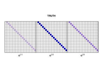
Figure 2: True autoregressive coefficients for the three segments used in the simulation scenario 1.

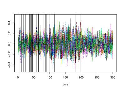
Figure 3: Estimated break points on the first stage for one of the runs in simulation scenario 1: Close to 18 points are selected in the first stage.

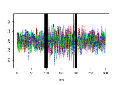
Figure 4: Final selected points for all the 100 runs from simulation scenario 1.

break points	truth	mean	std	selection rate
1	0.3333	0.3315	0.0074	1
2	0.6667	0.6632	0.0044	1

Table 1: Results of simulation scenario 1. The table shows mean and standard deviation of locations of selected break points, as well as the percentage of simulation runs where break points are correctly detected.

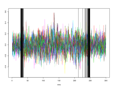
Figure 5: Final selected points for all the 100 runs from simulation scenario 2.

break points	truth	mean	std	selection rate
1	0.1	0.101	0.0082	0.98
2	0.8333	0.8134	0.0226	1

Table 2: Results of simulation scenario 2. The table shows mean and standard deviation of locations of selected break points, as well as the percentage of simulation runs where break points are correctly detected.

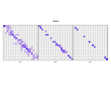
Figure 6: True autoregressive coefficients for the three segments used in the simulation scenario 3.

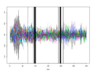
Figure 7: Final selected points for all the 100 runs from simulation scenario 3.

break points	truth	mean	std	selection rate
1	0.3333	0.3282	0.0153	0.92
2	0.6667	0.6601	0.01	0.98

Table 3: Results of simulation scenario 3. The table shows mean and standard deviation of locations of selected break points, as well as the percentage of simulation runs where break points are correctly detected.

5 Real Data Applications

In this section, we apply the proposed model to two real data sets in order to illustrate its performance in detecting break points in different settings.

5.1 EEG Data

The data considered in this application consists of electroencephalogram (EEG) signals recorded at 18 locations on the scalp of a patient diagnosed with left temporal lobe epilepsy during an epileptic seizure. The sampling rate is 100 Hz and the total number of time points per EEG is $T=32,768$ over 238 seconds. The time series for all 18 EEG channels are shown in Figure 1. The seizure was estimated to take place at $t=185s$. Examining the EEG plots, it can be seen that the magnitude and the volatility of signals change simultaneously around that time.

To speed up the computations in this analysis, we selected one observation per second and reduced the total time points to $T=328$. The EEG from a specific channel (P3) was previously used in Davis et al., (2006) and Chan et al., (2014). Table 4 shows the location of the selected break points using the Auto–PARM method of Davis et al., (2006), the two-stage procedure of Chan et al., (2014) based on data from channel P3, and our proposed multivariate method. Our method correctly detects a break point at at $t=186$, which is close to the seizure time identified by neurologists. The majority of other selected break points by our method are close to the break points detected by the two univariate approaches.

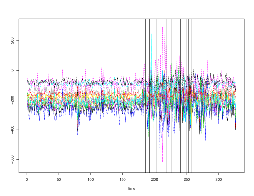
Figure 8: EEG data over 328 seconds with the 10 selected break points.

Methods	1	2	3	4	5	6	7	8	9	10	11
Auto–PARM	186	190	206	221	233	249	262	275	306	308	326
Chan (2014)	184	206	220	234	255	277	306	325	–	–	–
Our method	80	186	192	202	219	227	240	249	253	258	–

Table 4: Location of break points detected in the EEG data using three different methods. The locations are rounded to the closest integer.

5.2 Yellow Cab Demand in NYC

As a second example, we apply our method to the yellow cab demand data in NYC. Here, the number of yellow cab pickups are aggregated spatially over the zipcodes and temporally over 15 minute intervals during April 16th, 2014. We only consider the zipcodes with more than 50 cab calls to obtain a better approximation using normal distribution. This results in 39 time series for zipcodes observed over 96 time points. To identify structural break points, we consider a differenced version of the data to remove first order non-stationarities. Table 5 shows the 10 break points detected for this data; the differenced time series and the detected break points are also shown in Figure 9.

Based on data from New York City metro (MTA), morning rush hour traffic in the city occurs between 6:30 AM and 9:30 AM, whereas the afternoon rush hour starts from 3:30 PM. Interestingly, among the selected break points, there are very close to the rush hour start/end dates during a typical day. Specifically, the selected break points at 7 AM, 10 AM, 3:30 PM, and 6 PM are close to rush hour periods in NYC. These results suggest that the covariance structure of cab demands between the zipcodes in NYC may significantly change before and after the rush hour periods.

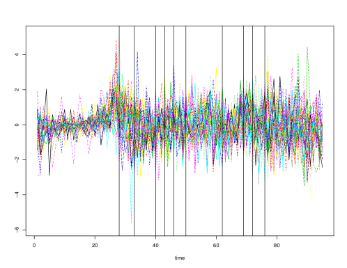
Figure 9: Plot of the NYC Yellow Cab Demand differenced time series from 39 different zipcodes over a single day with 96 time points; the 10 selected break points by the proposed method are shown as vertical lines.

	1	2	3	4	5	6	7	8	9	10
Our method	7am	8:15am	10am	10:45am	11:30am	12:30am	3:30pm	5:15pm	6pm	7pm

Table 5: The location of break points for the NYC Yellow Cab Demand data.

6 Discussion

In this article, we developed a two-stage method for detecting structural break point in high-dimensional piecewise stationary VAR models. A block coordinate descent algorithm was developed to implement the proposed method efficiently.

We showed that the proposed method consistently detects the total number of the break points, as well as their locations. Numerical experiments through in three simulation settings and two real data applications corroborate these theoretical findings. In particular, in both real data sets, the break points detected using the proposed method are in agreement with the nature of the data sets.

When the total number of break points $m_{0}$ is finite, the rate of consistency for detecting break point locations relative to the sample size $T$ is affected by three factors: (1) the number of time points $T$, (2) the number of time series observed $p$, (3) the total sparsity of the model $d_{n}^{\star}$. For the univariate case, this rate was shown to be of order $({\log n})/{n}$ by Chan et al., (2014). In the high-dimensional case, the rate is shown here to be of order $({d_{n}^{\star}\log n\log p})/{n}$. This rate puts an upper bound on the number of time series observed and the total sparsity in the model in the high-dimensional setting. Moreover, the proposed procedure allows for the number of break points to increase with the sample size, as long as the minimum distance between consecutive break points is large enough (Assumptions $A3$ and $A4$ connect the consistency rate of break point detection with the minimum distance between consecutive break points). Extending the methodology and theory in this paper to high-dimensional threshold autoregressive (TAR) models (Tsay, 1989) can offer an interesting direction of future research.

Appendix

This section collects the technical lemmas, as well as the proofs of the main results in the paper.

Appendix A: Technical Lemmas

Lemma 1.

There exist constants $c_{i}>0$ such that for $n\geq c_{0}\left(\log(n)+2\log(p)+\log(d)\right)$, with probability at least $1-c_{1}\exp\left(-c_{2}\left(\log(n)+2\log(p)+\log(d)\right)\right)$, we have

$$\left|\left|\frac{Z^{\prime}E}{n}\right|\right|_{\infty}\leq c_{3}\sqrt{\frac{\log(n)+2\log(p)+\log(d)}{n}}$$ (12)

Proof.

Note that $\frac{1}{n}Z^{\prime}E=\frac{1}{n}(I_{p}\otimes\mathcal{X}^{\prime})E=\mbox{vec}(\mathcal{X}^{\prime}\varepsilon(n))/n$. Let $\mathcal{X}(h,.)$ and $\mathcal{X}(h,l)$ be the $h$-th block column and the $l$-th column of the $h$-th block column of $\mathcal{X}$, respectively, $1\leq h\leq n$, $1\leq l\leq d$. More specifically,

$$\mathcal{X}(h,.)=\begin{pmatrix}&0&\\ &\vdots&\\ &0&\\ y_{d+h-2}^{\prime}&\ldots&y_{h-1}^{\prime}\\ &\vdots&\\ y_{T-1}^{\prime}&\ldots&y_{T-d}^{\prime}\end{pmatrix}_{n\times pd},\hskip 28.45274pt\mathcal{X}(h,l)=\begin{pmatrix}0\\ \vdots\\ 0\\ y_{d+h-l-1}^{\prime}\\ \vdots\\ y_{T-l}^{\prime}\end{pmatrix}_{n\times p}.$$ (13)

Now,

$$\left|\left|\frac{Z^{\prime}E}{n}\right|\right|_{\infty}=\max_{1\leq h\leq n,1\leq l\leq d,1\leq i,j\leq p}\left|e_{i}^{\prime}\left(\frac{\mathcal{X}^{\prime}(h,l)\varepsilon(n)}{n}\right)e_{j}\right|,$$ (14)

where $e_{i}\in\mathbb{R}^{p}$ with the $i$-th element equals to 1 and zero on the rest. Note that,

$$\frac{\mathcal{X}^{\prime}(h,l)\varepsilon(n)}{n}=\frac{1}{n}\sum_{j=h-l-1}^{T-d-l}y_{d+j}\varepsilon^{\prime}_{d+j+l}.$$

Now. sine $\mbox{cov}(y_{d+j},\varepsilon_{d+j+l})=0$ for all $j,l,h$, similar argument as in proposition 2.4 (b) of (Basu & Michailidis, (2015)) shows that for fixed $i,j,h,l$, there exist $k_{1},k_{2}>0$ such that for all $\eta>0$:

$$\mathbb{P}\left(\left|e_{i}^{\prime}\left(\frac{\mathcal{X}^{\prime}(h,l)\varepsilon(n)}{n}\right)e_{j}\right|>k_{1}\eta\right)\leq 6\exp\left(-k_{2}n\min(\eta,\eta^{2})\right).$$

Set $\eta=k_{3}\sqrt{\frac{\log(n)+2\log(p)+\log(d)}{n}}$ for a large enough $k_{3}>0$, and taking the union over the $q=np^{2}d$ possible choices of $i,j,h,l$ yield the result. ∎

Lemma 2.

Let $\widehat{\Theta}$ be defined as in (4), then under the assumptions of theorem (1):

$$\sum_{l=\widehat{t}_{j}}^{n}Y_{l-1}\left(y_{l}^{\prime}-Y_{l-1}^{\prime}\sum_{i=1}^{l}\widehat{\theta}_{i}^{\prime}\right)=\frac{n\lambda_{n}}{2}\mbox{sign}(\widehat{\theta}_{\widehat{t}_{j}}^{\prime}),\hskip 28.45274pt\mbox{for}\,\,\,j=1,2,...,\widehat{m},$$ (15)

where $Y_{l}^{\prime}=\left(y_{l}^{\prime}\ldots y_{l-d+1}^{\prime}\right)_{1\times pd}$, and

$$\left|\left|\sum_{l=j}^{n}Y_{l-1}\left(y_{l}^{\prime}-Y_{l-1}^{\prime}\sum_{i=1}^{l}\widehat{\theta}_{i}^{\prime}\right)\right|\right|_{\infty}\leq\frac{n\lambda_{n}}{2},\hskip 28.45274pt\mbox{for}\,\,\,j=d-1,2,...,n.$$ (16)

Moreover, $\sum_{i=1}^{t}\widehat{\theta}_{i}=\widehat{\Phi}^{(.,j)}$ for $\widehat{t}_{j-1}\leq t\leq\widehat{t}_{j}-1$, $j=1,2,...,|\mathcal{A}_{n}|$.

Proof.

This is just checking the KKT condition of the proposed optimization problem. ∎

Lemma 3.

Under assumption A1, there exist constants $c_{i}>0$ such that with probability at least $1-c_{1}\exp(-c_{2}(\log(d)+2\log(p)))$,

$$\sup_{1\leq i\leq m_{0},s\geq t_{i},|t_{i}-s|>n\gamma_{n}}\left|\left|{(t_{i}-s)}^{-1}\left(\sum_{l=s}^{t_{i}-1}Y_{l-1}Y_{l-1}^{\prime}-\Gamma_{i}^{d}(0)\right)\right|\right|_{\infty}\leq c_{3}\sqrt{\frac{\log(d)+2\log(p)}{n\gamma_{n}}},$$ (17)

where $\Gamma_{i}^{d}(0)=\mathbb{E}(Y_{l-1}Y_{l-1}^{\prime})$, and

$$\sup_{1\leq i\leq m_{0},s\geq t_{i},|t_{i}-s|>n\gamma_{n}}\left|\left|{(t_{i}-s)}^{-1}\sum_{l=s}^{t_{i}-1}Y_{l-1}\varepsilon_{l}^{\prime}\right|\right|_{\infty}\leq c_{3}\sqrt{\frac{\log(d)+2\log(p)}{n\gamma_{n}}}.$$ (18)

Proof.

The proof of this lemma is similar to proposition 2.4 in Basu & Michailidis, (2015). Here we briefly mention the proof omitting the details. For the first one, note that using similar argument as in proposition 2.4 (a) in Basu & Michailidis, (2015), there exist $k_{1},k_{2}>0$ such that for each fixed $i,j=1,...,pd$,

$$\mathbb{P}\left(\left|e_{i}^{\prime}\frac{\sum_{l=s}^{t_{i}-1}Y_{l-1}Y_{l-1}^{\prime}-\Gamma_{i}^{d}(0)}{t_{i}-s}e_{j}\right|>k_{1}\eta\right)\leq 6\exp(-k_{2}n\gamma_{n}\min(\eta,\eta^{2})).$$ (19)

Setting $\eta=k_{3}\sqrt{\frac{\log(dp^{2})}{n\gamma_{n}}}$, and taking the union over all possible values of $i,j$, we get the first part. For the second part, the proof will be similar to lemma (1). Again, there exist $k_{1},k_{2}>0$ such that for each fixed $i=1,...,pd$, $j=1,...,p$,

$$\mathbb{P}\left(\left|e_{i}^{\prime}\frac{\sum_{l=s}^{t_{i}-1}Y_{l-1}\varepsilon_{l}^{\prime}}{t_{i}-s}e_{j}\right|>k_{1}\eta\right)\leq 6\exp(-k_{2}n\gamma_{n}\min(\eta,\eta^{2})).$$ (20)

Setting $\eta=k_{3}\sqrt{\frac{\log(dp^{2})}{n\gamma_{n}}}$, and taking the union over all possible values of $i,j$, we get:

$$\left|\left|{(t_{i}-s)}^{-1}\left(\sum_{l=s}^{t_{i}-1}Y_{l-1}Y_{l-1}^{\prime}-\Gamma_{i}^{d}(0)\right)\right|\right|_{\infty}\leq c_{3}\sqrt{\frac{\log(d)+2\log(p)}{n\gamma_{n}}},$$ (21)

and

$$\left|\left|{(t_{i}-s)}^{-1}\sum_{l=s}^{t_{i}-1}Y_{l-1}\varepsilon_{l}^{\prime}\right|\right|_{\infty}\leq c_{3}\sqrt{\frac{\log(d)+2\log(p)}{n\gamma_{n}}},$$ (22)

with high probability converging to 1 for any $i=1,2,...,m_{0}$, as long as $|t_{i}-s|>n\gamma_{n}$ and $s\geq t_{i-1}$. Note that the constants $c_{1},c_{2},c_{3}$ can be chosen large enough and in such a way that the upper bounds above would be independent of the break point $t_{i}$. Therefore, we have the desired upper bounds verified with probability at least $1-c_{1}\exp(-c_{2}(\log(d)+2\log(p)))$. ∎

Lemma 4.

Under the assumptions of theorem (4), for $m<m_{0}$, there exists a constant $c>0$ such that:

$$\mathbb{P}\left(\min_{(s_{1},...,s_{m})\subset\{1,...,T\}}L_{n}(s_{1},s_{2},...,s_{m};\eta_{n})>\sum_{t=d}^{T}||\varepsilon_{t}||_{2}^{2}+c\Delta_{n}-M_{\Phi}(m_{0}+1)n\gamma_{n}d_{n}^{\star}\right)\rightarrow 1,$$ (23)

where $\Delta_{n}=\min_{1\leq j\leq m_{0}+1}|t_{j}-t_{j-1}|$.

Proof.

Since $m<m_{0}$, there exists a point $t_{j}$ such that $|s_{i}-t_{j}|>\Delta_{n}/4$. Now, $L_{n}(s_{1},s_{2},...,s_{m};\eta_{n})-n\,\eta_{n}\sum_{i=1}^{m+1}||\widehat{\theta}_{(s_{i-1},s_{i})}||_{1}=||\mathcal{Y}-\mathcal{X}_{s_{1},...,s_{m}}\widehat{\theta}_{s_{1},...,s_{m}}||_{F}^{2}=\sum_{i=1}^{m_{0}+2}T_{i}$, where $T_{i}$ is the sum of squares involving $Y_{k}$, $t_{i-1}\leq k<t_{i}$ for $i=1,...,j-1,j+2,...,m_{0}+1$, and $T_{j},T_{j+1},T_{m_{0}+2}$ are the sums of $Y_{k}$ for $t_{j-1}\leq k<t_{j}-\Delta_{n}/4$, $t_{j}+\Delta_{n}/4\leq k<t_{j+1}$, and $t_{j}-\Delta_{n}/4\leq k<t_{j}+\Delta_{n}/4$, respectively. For $i=1,...,j-1,j+2,...,m_{0}+1$, we find a lower bound for the $T_{i}$. For a fixed $i$, let’s say there are $r_{i}$ points within $[t_{i-1},t_{i})$, denoting them by $\{s_{l},s_{l+1},...,s_{l+r_{i}}\}\subset\{s_{1},...,s_{m}\}$, we put $r_{i}=-1$ if there are no points. Now, $T_{i}$ can be decomposed as:

$$T_{i}=\sum_{t=t_{i-1}}^{s_{l}-1}||y_{t}-\widehat{\theta}_{(t_{i-1},s_{l})}Y_{t-1}||_{2}^{2}+\sum_{h=l}^{l+r_{i}-1}\sum_{t=s_{h}}^{s_{h+1}-1}||y_{t}-\widehat{\theta}_{(s_{h},s_{h+1})}Y_{t-1}||_{2}^{2}+\sum_{t=s_{l+r_{i}}}^{t_{i}-1}||y_{t}-\widehat{\theta}_{(s_{l+r_{i}},t_{i})}Y_{t-1}||_{2}^{2}.$$ (24)

Note that for a fixed $h$,

$$\sum_{t=s_{h}}^{s_{h+1}-1}||y_{t}-\widehat{\theta}_{(s_{h},s_{h+1})}Y_{t-1}||_{2}^{2} = \sum_{t=s_{h}}^{s_{h+1}-1}||\varepsilon_{t}||_{2}^{2}+\sum_{t=s_{h}}^{s_{h+1}-1}||(\Phi^{(.,i)}-\widehat{\theta}_{(s_{h},s_{h+1})})Y_{t-1}||_{2}^{2}$$ (25)

$$+ 2\sum_{t=s_{h}}^{s_{h+1}-1}Y_{t-1}^{\prime}(\Phi^{(.,i)}-\widehat{\theta}_{(s_{h},s_{h+1})})^{\prime}\varepsilon_{t}.$$

Now, by similar arguments as in lemma (3), we have:

$$\left|\sum_{t=s_{h}}^{s_{h+1}-1}Y_{t-1}^{\prime}(\Phi^{(.,i)}-\widehat{\theta}_{(s_{h},s_{h+1})})^{\prime}\varepsilon_{t}\right| \leq \frac{||\sum_{t=s_{h}}^{s_{h+1}-1}Y_{t-1}\varepsilon_{t}^{\prime}||_{\infty}}{n\gamma_{n}}n\gamma_{n}||\Phi^{(.,i)}-\widehat{\theta}_{(s_{h},s_{h+1})}||_{1}$$ (26)

$$= o_{p}(n\gamma_{n})||\Phi^{(.,i)}-\widehat{\theta}_{(s_{h},s_{h+1})}||_{1},$$

which adds up to:

$$T_{i}\geq\sum_{t=t_{i-1}}^{t_{i}-1}||\varepsilon_{t}||_{2}^{2}-o_{p}(n\gamma_{n})\left(\sum_{h=l}^{l+r_{i}-1}||\Phi^{(.,i)}-\widehat{\theta}_{(s_{h},s_{h+1})}||_{1}+||\Phi^{(.,i)}-\widehat{\theta}_{(t_{i-1},s_{l})}||_{1}+||\Phi^{(.,i)}-\widehat{\theta}_{(s_{l+r_{i}},t_{i})}||_{1}\right).$$ (27)

Let’s focus on $T_{m_{0}+2}$. Since there are no points inside the interval $[t_{j}-\Delta_{n}/4,t_{j}+\Delta_{n}/4)$, $\widehat{\theta}_{(t_{j}-\Delta_{n}/4,t_{j})}=\widehat{\theta}_{(t_{j},t_{j}+\Delta_{n}/4)}=\theta^{\star}$. Now, we can decompose it as:

$$T_{m_{0}+2}=\sum_{t=t_{j}-\Delta_{n}/4}^{t_{j}-1}||y_{t}-\theta^{\star}Y_{t-1}||_{2}^{2}+\sum_{t=t_{j}}^{t_{j}+\Delta_{n}/4}||y_{t}-\theta^{\star}Y_{t-1}||_{2}^{2}=I+II.$$ (28)

We zoom in $I$:

$$I = \sum_{t=t_{j}-\Delta_{n}/4}^{t_{j}-1}||\varepsilon_{t}||_{2}^{2}+\sum_{t=t_{j}-\Delta_{n}/4}^{t_{j}-1}||(\Phi^{(.,j)}-\theta^{\star})Y_{t-1}||_{2}^{2}$$ (29)

$$+ 2\sum_{t=t_{j}-\Delta_{n}/4}^{t_{j}-1}Y_{t-1}^{\prime}(\Phi^{(.,j)}-\theta^{\star})^{\prime}\varepsilon_{t}$$

$$= \sum_{t=t_{j}-\Delta_{n}/4}^{t_{j}-1}||\varepsilon_{t}||_{2}^{2}+I_{A}+I_{B}.$$

Similar to (26), we have:

$$\left|I_{B}\right| \leq o_{p}(n\gamma_{n})||\Phi^{(.,j)}-\theta^{\star}||_{1},$$ (30)

We need to find a large enough bound for $I_{A}$. Denote the $i$-th row of $\Phi^{(.,j)}-\theta^{\star}$ by $v_{i}$ for $i=1,...,p$. Now,

$$I_{A} = \sum_{t=t_{j}-\Delta_{n}/4}^{t_{j}-1}Y_{t-1}^{\prime}(\Phi^{(.,j)}-\theta^{\star})^{\prime}(\Phi^{(.,j)}-\theta^{\star})Y_{t-1}$$ (31)

$$= \mbox{tr}\left((\Phi^{(.,j)}-\theta^{\star})\left(\sum_{t=t_{j}-\Delta_{n}/4}^{t_{j}-1}Y_{t-1}Y_{t-1}^{\prime}\right)(\Phi^{(.,j)}-\theta^{\star})^{\prime}\right)$$

$$= \sum_{i=1}^{p}v_{i}\left(\sum_{t=t_{j}-\Delta_{n}/4}^{t_{j}-1}Y_{t-1}Y_{t-1}^{\prime}\right)v_{i}^{\prime}$$

$$= \sum_{i=1}^{p}v_{i}\left(\sum_{t=t_{j}-\Delta_{n}/4}^{t_{j}-1}\left(Y_{t-1}Y_{t-1}^{\prime}-\Gamma_{j}(0)\right)+\frac{\Delta_{n}}{4}\Gamma_{j}(0)\right)v_{i}^{\prime}$$

By similar arguments as in lemma (3), we have:

$$\frac{4}{\Delta_{n}}\left|\left|\sum_{t=t_{j}-\Delta_{n}/4}^{t_{j}-1}\left(Y_{t-1}Y_{t-1}^{\prime}-\Gamma_{j}(0)\right)\right|\right|_{\infty}=o_{p}(1).$$

Using the above fact,

$$I_{A}\geq\frac{\Delta_{n}}{8}\Lambda_{\min}(\Gamma_{j}(0))\sum_{i=1}^{p}||v_{i}||_{2}^{2}=c_{1}||\Phi^{(.,j)}-\theta^{\star}||_{2}^{2},$$ (32)

with $c_{1}=\frac{1}{8}\min_{1\leq j\leq m_{0}+1}\Lambda_{\min}(\Gamma_{j}(0))$. All combined lead to:

$$I\geq\sum_{t=t_{j}-\Delta_{n}/4}^{t_{j}-1}||\varepsilon_{t}||_{2}^{2}+c_{1}||\Phi^{(.,j)}-\theta^{\star}||_{2}^{2}-o_{p}(n\gamma_{n})||\Phi^{(.,j)}-\theta^{\star}||_{1}.$$ (33)

Similarly, one can show that:

$$II\geq\sum_{t=t_{j}}^{t_{j}+\Delta_{n}/4}||\varepsilon_{t}||_{2}^{2}+c_{1}||\Phi^{(.,j+1)}-\theta^{\star}||_{2}^{2}-o_{p}(n\gamma_{n})||\Phi^{(.,j+1)}-\theta^{\star}||_{1}.$$ (34)

Now, since $\min_{1\leq j\leq m_{0}}\left|\left|\Phi^{(.,j+1)}-\Phi^{(.,j)}\right|\right|_{2}\geq v>0$, we have:

$$T_{m_{0}+2}=I+II\geq\sum_{t=t_{j}-\Delta_{n}/4}^{t_{j}+\Delta_{n}/4}||\varepsilon_{t}||_{2}^{2}+c\Delta_{n}-o_{p}(n\gamma_{n})\left(||\Phi^{(.,j)}-\theta^{\star}||_{1}+||\Phi^{(.,j+1)}-\theta^{\star}||_{1}\right),$$ (35)

where $c=c_{1}\nu$. Now, since we don’t know which true segments will be inside each estimated segment, we have the following lower bound:

$$L_{n}(s_{1},s_{2},...,s_{m};\eta_{n})-n\,\eta_{n}\sum_{i=1}^{m+1}||\widehat{\theta}_{(s_{i-1},s_{i})}||_{1}=\sum_{i=1}^{m_{0}+2}T_{i}\geq\sum_{t=d}^{T}||\varepsilon_{t}||_{2}^{2}+c\Delta_{n}-o_{p}(n\gamma_{n})\sum_{i=1}^{m+1}\sum_{j=1}^{m_{0}+1}||\Phi^{(.,j)}-\widehat{\theta}_{(s_{i-1},s_{i})}||_{1}.$$ (36)

Now, by assumption A4 (a) or (b), we have:

$$L_{n}(s_{1},s_{2},...,s_{m};\eta_{n}) \geq \sum_{t=d}^{T}||\varepsilon_{t}||_{2}^{2}+c\Delta_{n}-(m_{0}+1)n\gamma_{n}\sum_{j=1}^{m_{0}+1}||\Phi^{(.,j)}||_{1}$$ (37)

$$\geq \sum_{t=d}^{T}||\varepsilon_{t}||_{2}^{2}+c\Delta_{n}-M_{\Phi}(m_{0}+1)n\gamma_{n}d_{n}^{\star},$$

with high probability approaching to 1. Note that the lower bound doesn’t depend on the choices of $s_{i}$’s as long as $m<m_{0}$. This completes the proof. ∎

Appendix B: Proof of Main Results

Proof of Theorem 1.

By definition of $\widehat{\Theta}$, we get

$$\frac{1}{n}||Y-Z\widehat{\Theta}||_{2}^{2}+\lambda_{n}\sum_{i=1}^{n}||\widehat{\theta}_{i}||_{1}\leq\frac{1}{n}||Y-Z\Theta||_{2}^{2}+\lambda_{n}\sum_{i=1}^{n}||\theta_{i}||_{1}.$$ (38)

Denoting $\mathcal{A}=\{t_{1},t_{1},...,t_{m_{0}}\}$, we have:

$$\frac{1}{n}\left|\left|Z\left(\widehat{\Theta}-\Theta\right)\right|\right|_{2}^{2} \leq \frac{2}{n}\left(\widehat{\Theta}-\Theta\right)^{\prime}Z^{\prime}E+\lambda_{n}\sum_{i=1}^{n}||\widehat{\theta}_{i}||_{1}-\lambda_{n}\sum_{i=1}^{n}||\theta_{i}||_{1}$$ (39)

$$\leq 2\left|\left|\frac{Z^{\prime}E}{n}\right|\right|_{\infty}\sum_{i=1}^{n}||\theta_{i}-\widehat{\theta}_{i}||_{1}+\lambda_{n}\sum_{i\in\mathcal{A}}\left(||\theta_{i}||_{1}-||\widehat{\theta}_{i}||_{1}\right)-\lambda_{n}\sum_{i\in\mathcal{A}^{c}}||\widehat{\theta}_{i}||_{1}$$

$$= \lambda_{n}\sum_{i\in\mathcal{A}}||\theta_{i}-\widehat{\theta}_{i}||_{1}+\lambda_{n}\sum_{i\in\mathcal{A}}\left(||\theta_{i}||_{1}-||\widehat{\theta}_{i}||_{1}\right)$$

$$\leq 2\lambda_{n}\sum_{i\in\mathcal{A}}||\theta_{i}||_{1}$$

$$\leq 2\lambda_{n}m_{n}\max_{1\leq j\leq m_{0}+1}\left|\left|\Phi^{(.,j)}-\Phi^{(.,j-1)}\right|\right|_{1}$$

$$= 4Cm_{n}\max_{1\leq j\leq m_{0}+1}\left\{\sum_{i=1}^{p}\left(s_{ij}+s_{i(j-1)}\right)\right\}M_{\Phi}\sqrt{\frac{\log(n)+2\log(p)+\log(d)}{n}},$$

with high probability approaching to 1 due to the lemma (1). ∎

Proof of Theorem 2.

The proof is similar to theorem 2.2 in (Chan et al., (2014)) and proposition 5 in (Harchaoui & Lévy-Leduc, (2010)). Before we start, define for a matrix $A\in\mathbb{R}^{pd\times p}$, $||A||_{\infty,NZ}=\max_{j\in NZ,1\leq i\leq p}|a_{ji}|$. Now, if for some $i=1,...,m_{0}$, $|\widehat{t}_{i}-t_{i}|>n\gamma_{n}$, this means that there exists a true break point $t_{i_{0}+1}$ which is isolated from all the estimated points, i.e. $\min_{1\leq i\leq m_{0}}|\widehat{t}_{i}-t_{i_{0}+1}|>n\gamma_{n}$. In other words, there exists an estimated break point $\widehat{t}_{j}$ such that, $t_{i_{0}+1}-t_{i_{0}}\vee\widehat{t}_{j}\geq n\gamma_{n}$ and $t_{i_{0}+2}\wedge\widehat{t}_{j+1}\geq n\gamma_{n}$. Apply lemma (2) twice to get:

$$\left|\left|\sum_{l=t_{i_{0}}\vee\widehat{t}_{j}}^{t_{i_{0}+1}-1}Y_{l-1}Y_{l-1}^{\prime}\left({\Phi^{\prime}}^{(.,i_{0}+1)}-\widehat{\Phi^{\prime}}^{(.,j+1)}\right)\right|\right|_{\infty,NZ}\leq n\lambda_{n}+\left|\left|\sum_{l=t_{i_{0}}\vee\widehat{t}_{j}}^{t_{i_{0}+1}-1}Y_{l-1}\varepsilon_{l}^{\prime}\right|\right|_{\infty}$$ (40)

and

$$\left|\left|\sum_{l=t_{i_{0}+1}}^{t_{i_{0}+2}\wedge\widehat{t}_{j+1}-1}Y_{l-1}Y_{l-1}^{\prime}\left({\Phi^{\prime}}^{(.,i_{0}+2)}-\widehat{\Phi^{\prime}}^{(.,j+1)}\right)\right|\right|_{\infty,NZ}\leq n\lambda_{n}+\left|\left|\sum_{l=t_{i_{0}+1}}^{t_{i_{0}+2}\wedge\widehat{t}_{j+1}-1}Y_{l-1}\varepsilon_{l}^{\prime}\right|\right|_{\infty}.$$ (41)

Now, consider the first equation (40). We can write the left hand side as

$$(t_{i_{0}+1}-t_{i_{0}}\vee\widehat{t}_{j})^{-1}\left|\left|\sum_{l=t_{i_{0}}\vee\widehat{t}_{j}}^{t_{i_{0}+1}-1}Y_{l-1}Y_{l-1}^{\prime}\left({\Phi^{\prime}}^{(.,i_{0}+1)}-\widehat{\Phi^{\prime}}^{(.,j+1)}\right)\right|\right|_{\infty,NZ} \geq \left|\left|(\Gamma_{i}^{d}(0)-A)\left({\Phi^{\prime}}^{(.,i_{0}+1)}\right)\right|\right|_{\infty,NZ}$$ (42)

$$- \left|\left|(\Gamma_{i}^{d}(0)-A)\left(\widehat{\Phi^{\prime}}^{(.,j+1)}\right)\right|\right|_{\infty},$$

for some random matrix $A$ with $||A||_{\infty}\rightarrow 0$ with high probability converging to one based on lemma (3). Then, we can show that based on the properties of the covariance matrix $\Gamma_{i}^{d}(0)$ that:

$$\left|\left|(\Gamma_{i}^{d}(0)-A)\left({\Phi^{\prime}}^{(.,i_{0}+1)}\right)\right|\right|_{\infty,NZ}\geq c_{1}(s^{\star})^{-1}\max_{1\leq i\leq p}\left|\left|\Phi_{i}^{(.,i_{0}+1)}\right|\right|_{2},$$ (43)

and

$$\left|\left|(\Gamma_{i}^{d}(0)-A)\left(\widehat{\Phi^{\prime}}^{(.,j+1)}\right)\right|\right|_{\infty}\leq c_{2}\left|\left|\widehat{\Phi^{\prime}}^{(.,j+1)}\right|\right|_{1},$$ (44)

for some positive constants $c_{1},c_{2}$. Putting them all together, and use lemma (3) again for for the second term on the right hand side of equation (40), we have:

$$c_{1}\max_{1\leq i\leq p}\left|\left|\Phi_{i}^{(.,i_{0}+1)}\right|\right|_{2}-c_{2}s^{\star}\left|\left|\widehat{\Phi^{\prime}}^{(.,j+1)}\right|\right|_{1}\leq\frac{s^{\star}n\lambda_{n}}{(t_{i_{0}+1}-t_{i_{0}}\vee\widehat{t}_{j})}+k_{1}s^{\star}\sqrt{\frac{\log p}{n\gamma_{n}}}.$$ (45)

The right hand side goes to zero based on A2 and A3. Similarly, we can use equation (41) to show that

$$c_{3}\max_{1\leq i\leq p}\left|\left|\Phi_{i}^{(.,i_{0}+2)}\right|\right|_{2}-c_{4}s^{\star}\left|\left|\widehat{\Phi^{\prime}}^{(.,j+1)}\right|\right|_{1}\leq\frac{s^{\star}n\lambda_{n}}{(t_{i_{0}+1}-t_{i_{0}}\vee\widehat{t}_{j})}+k_{1}s^{\star}\sqrt{\frac{\log p}{n\gamma_{n}}}.$$ (46)

Putting them together implies that:

$$\frac{\max_{1\leq i\leq p}\left|\left|\Phi_{i}^{(.,i_{0}+2)}\right|\right|_{2}}{\max_{1\leq i\leq p}\left|\left|\Phi_{i}^{(.,i_{0}+1)}\right|\right|_{2}}\leq c_{5},$$ (47)

and so, if we choose the $\nu^{\prime}$ large enough in A2, we reach the contradiction. This completes the proof.

∎

Proof of Theorem 3.

The proof is similar to the proof of theorem 2.3 in Chan et al., (2014). Here we will mention the proof of the first part. For that, assume $|\mathcal{A}_{n}|<m_{0}$. This means there exist an isolated true break point, say $t_{i_{0}}$. More specifically, there exists an estimated break point $\widehat{t}_{j}$ such that, $t_{i_{0}+1}-t_{i_{0}}\vee\widehat{t}_{j}\geq n\gamma_{n}/3$ and $t_{i_{0}+2}\wedge\widehat{t}_{j+1}\geq n\gamma_{n}/3$. Apply lemma (2) twice to get:

$$\left|\left|\sum_{l=t_{i_{0}}\vee\widehat{t}_{j}}^{t_{i_{0}+1}-1}Y_{l-1}Y_{l-1}^{\prime}\left({\Phi^{\prime}}^{(.,i_{0}+1)}-\widehat{\Phi^{\prime}}^{(.,j+1)}\right)\right|\right|_{\infty,NZ}\leq n\lambda_{n}+\left|\left|\sum_{l=t_{i_{0}}\vee\widehat{t}_{j}}^{t_{i_{0}+1}-1}Y_{l-1}\varepsilon_{l}^{\prime}\right|\right|_{\infty}$$ (48)

and

$$\left|\left|\sum_{l=t_{i_{0}+1}}^{t_{i_{0}+2}\wedge\widehat{t}_{j+1}-1}Y_{l-1}Y_{l-1}^{\prime}\left({\Phi^{\prime}}^{(.,i_{0}+2)}-\widehat{\Phi^{\prime}}^{(.,j+1)}\right)\right|\right|_{\infty,NZ}\leq n\lambda_{n}+\left|\left|\sum_{l=t_{i_{0}+1}}^{t_{i_{0}+2}\wedge\widehat{t}_{j+1}-1}Y_{l-1}\varepsilon_{l}^{\prime}\right|\right|_{\infty}.$$ (49)

Now, similar argument as in theorem (2) reaches to contradiction, and this completes the proof. ∎

Proof of Theorem 4.

Let’s focus on the first part. We show that (a) $\mathbb{P}(\widehat{\widehat{m}}<m_{0})\rightarrow 0$, and (b) $\mathbb{P}(\widehat{\widehat{m}}>m_{0})\rightarrow 0$. For the first claim, from theorem (3), we know that there are points $\widehat{t}_{i}\in\mathcal{A}_{n}$ such that $\max_{1\leq i\leq m_{0}}|\widehat{t}_{i}-t_{i}|\leq n\gamma_{n}$. The parameter estimated when choosing these $m_{0}$ points are $\widehat{\theta}_{(\widehat{t}_{1},...,\widehat{t}_{m_{0}})}$. By the definition of this parameter, it minimizes the least squares plus the $L_{1}$ penalty on its norm. Therefore, it has to beat the case where one puts $\Phi^{(.,j)}$ on the segment $[\widehat{t}_{j-1},\widehat{t}_{j})$ for $j=1,...,m_{0}+1$. This leads to an upper bound for $L(\widehat{t}_{1},...,\widehat{t}_{m_{0}};\eta_{n})$. By similar arguments as in lemma (4), we get that there exist constants $K_{1},K_{2},K>0$ such that:

$$L(\widehat{t}_{1},...,\widehat{t}_{m_{0}};\eta_{n}) \leq \sum_{t=d}^{T}||\varepsilon_{t}||_{2}^{2}+o_{p}(n\gamma_{n})\sum_{j=1}^{m_{0}}\left|\left|\Phi^{(.,j+1)}-\Phi^{(.,j)}\right|\right|_{1}$$ (50)

$$+ K_{1}n\gamma_{n}\sum_{j=1}^{m_{0}}\left|\left|\Phi^{(.,j+1)}-\Phi^{(.,j)}\right|\right|_{2}^{2}+K_{2}n\gamma_{n}\sum_{j=1}^{m_{0}+1}\left|\left|\Phi^{(.,j+1)}\right|\right|_{1}$$

$$\leq \sum_{t=d}^{T}||\varepsilon_{t}||_{2}^{2}+Kn\gamma_{n}d_{n}^{\star}.$$

Now,

$$IC(\widehat{\widehat{t}}_{1},...,\widehat{\widehat{t}}_{\widehat{\widehat{m}}}) = L_{n}(\widehat{\widehat{t}}_{1},...,\widehat{\widehat{t}}_{\widehat{\widehat{m}}};\eta_{n})+\widehat{\widehat{m}}\omega_{n}$$ (51)

$$> \sum_{t=d}^{T}||\varepsilon_{t}||_{2}^{2}+c\Delta_{n}-M_{\Phi}(m_{0}+1)n\gamma_{n}d_{n}^{\star}+\widehat{\widehat{m}}\omega$$

$$\geq L(\widehat{t}_{1},...,\widehat{t}_{m_{0}};\eta_{n})+m_{0}\omega_{n}+c\Delta_{n}-K_{3}(m_{0}+1)n\gamma_{n}d_{n}^{\star}-(m_{0}-\widehat{\widehat{m}})\omega_{n}$$

$$\geq L(\widehat{t}_{1},...,\widehat{t}_{m_{0}};\eta_{n})+m_{0}\omega_{n},$$

since $\lim_{n\rightarrow\infty}n\gamma_{n}d_{n}^{\star}/\omega_{n}\leq 1$, and $\lim_{n\rightarrow\infty}m_{0}\omega_{n}/\Delta_{n}=0$. This proves part (a). To prove part (b), note that a similar argument as in lemma (4) shows that

$$L_{n}(\widehat{\widehat{t}}_{1},...,\widehat{\widehat{t}}_{\widehat{\widehat{m}}};\eta_{n})\geq\sum_{t=d}^{T}||\varepsilon_{t}||_{2}^{2}-K_{4}mn\gamma_{n}d_{n}^{\star},$$ (52)

for some constant $K_{4}>0$. A comparison between $IC(\widehat{\widehat{t}}_{1},...,\widehat{\widehat{t}}_{\widehat{\widehat{m}}})$ and $IC(\widehat{t}_{1},...,\widehat{t}_{m_{0}})$ yields to:

$$\sum_{t=d}^{T}||\varepsilon_{t}||_{2}^{2}-K_{4}mn\gamma_{n}d_{n}^{\star}+m\omega_{n} \leq IC(\widehat{\widehat{t}}_{1},...,\widehat{\widehat{t}}_{\widehat{\widehat{m}}})$$ (53)

$$\leq IC(\widehat{t}_{1},...,\widehat{t}_{m_{0}})$$

$$\leq \sum_{t=d}^{T}||\varepsilon_{t}||_{2}^{2}+Kn\gamma_{n}d_{n}^{\star}+m_{0}\omega_{n},$$

which means:

$$(m-m_{0})\omega_{n}\leq K_{4}mn\gamma_{n}d_{n}^{\star}+Kn\gamma_{n}d_{n}^{\star},$$ (54)

which contradicts with the fact that $m_{0}n\gamma_{n}d_{n}^{\star}/\omega_{n}\rightarrow 0$. This completes the first part of the theorem.

For the second part, put $B=2K/c$. Now, suppose that there exists a point $t_{i}$ such that $\min_{1\leq j\leq m_{0}}|\widehat{\widehat{t}}_{j}-t_{j}|\geq Bn\gamma_{n}d_{n}^{\star}$. Then, by similar argument as in lemma (4), we can show that:

$$\sum_{t=d}^{T}||\varepsilon_{t}||_{2}^{2}+cBn\gamma_{n}d_{n}^{\star} < L_{n}(\widehat{\widehat{t}}_{1},...,\widehat{\widehat{t}}_{m_{0}})$$ (55)

$$\leq L_{n}(\widehat{t}_{1},...,\widehat{t}_{m_{0}})$$

$$\leq \sum_{t=d}^{T}||\varepsilon_{t}||_{2}^{2}+Kn\gamma_{n}d_{n}^{\star},$$

which contradicts with the way $B$ was selected. This completes the proof of the whole theorem. ∎

References

- Bai, (1997) Bai, Jushan. 1997. Estimation of a change point in multiple regression models. The review of economics and statistics, 79(4), 551–563.
- Basu & Michailidis, (2015) Basu, Sumanta, & Michailidis, George. 2015. Regularized estimation in sparse high-dimensional time series models. The Annals of Statistics, 43(4), 1535–1567.
- Bickel et al., (2009) Bickel, Peter J, Ritov, Ya acov, & Tsybakov, Alexandre B. 2009. Simultaneous analysis of LASSO and Dantzig selector. The Annals of Statistics, 37(4), 1705–1732.
- Boysen et al., (2009) Boysen, Leif, Kempe, Angela, Liebscher, Volkmar, Munk, Axel, & Wittich, Olaf. 2009. Consistencies and rates of convergence of jump-penalized least squares estimators. The Annals of Statistics, 157–183.
- Chan et al., (2014) Chan, Ngai Hang, Yau, Chun Yip, & Zhang, Rong-Mao. 2014. Group LASSO for structural break time series. Journal of the American Statistical Association, 109(506), 590–599.
- Chen et al., (2016) Chen, Shizhe, Shojaie, Ali, & Witten, Daniela M. 2016. Network Reconstruction From High Dimensional Ordinary Differential Equations. Journal of the American Statistical Association.
- Chen et al., (2017) Chen, Shizhe, Witten, Daniela, Shojaie, Ali, et al. 2017. Nearly assumptionless screening for the mutually-exciting multivariate Hawkes process. Electronic Journal of Statistics, 11(1), 1207–1234.
- Chen et al., (2013) Chen, Xiaohui, Xu, Mengyu, & Wu, Wei Biao. 2013. Covariance and precision matrix estimation for high-dimensional time series. The Annals of Statistics, 41(6), 2994–3021.
- Clarida et al., (2000) Clarida, Richard, Gali, Jordi, & Gertler, Mark. 2000. Monetary policy rules and macroeconomic stability: evidence and some theory. The Quarterly journal of economics, 115(1), 147–180.
- Dahlhaus, (2012) Dahlhaus, Rainer. 2012. Locally stationary processes. Handbook of statistics, 30, 351–412.
- Davis et al., (2006) Davis, Richard A, Lee, Thomas C M, & Rodriguez-Yam, Gabriel A. 2006. Structural break estimation for nonstationary time series models. Journal of the American Statistical Association, 101(473), 223–239.
- De Mol et al., (2008) De Mol, Christine, Giannone, Domenico, & Reichlin, Lucrezia. 2008. Forecasting using a large number of predictors: Is Bayesian shrinkage a valid alternative to principal components? Journal of Econometrics, 146(2), 318–328.
- Ding et al., (2016) Ding, Xin, Qiu, Ziyi, & Chen, Xiaohui. 2016. Sparse transition matrix estimation for high-dimensional and locally stationary vector autoregressive models. arXiv preprint arXiv:1604.04002.
- Fan et al., (2011) Fan, Jianqing, Lv, Jinchi, & Qi, Lei. 2011. Sparse high-dimensional models in economics.
- Fujita et al., (2007) Fujita, André, Sato, João R, Garay-Malpartida, Humberto M, Yamaguchi, Rui, Miyano, Satoru, Sogayar, Mari C, & Ferreira, Carlos E. 2007. Modeling gene expression regulatory networks with the sparse vector autoregressive model. BMC Systems Biology, 1(1), 39.
- Hall et al., (2016) Hall, Eric C, Raskutti, Garvesh, & Willett, Rebecca. 2016. Inference of High-dimensional Autoregressive Generalized Linear Models. arXiv preprint arXiv:1605.02693.
- Hansen et al., (2015) Hansen, Niels Richard, Reynaud-Bouret, Patricia, Rivoirard, Vincent, et al. 2015. Lasso and probabilistic inequalities for multivariate point processes. Bernoulli, 21(1), 83–143.
- Harchaoui & Lévy-Leduc, (2010) Harchaoui, Zaıd, & Lévy-Leduc, Céline. 2010. Multiple change-point estimation with a total variation penalty. Journal of the American Statistical Association, 105(492), 1480–1493.
- Lu et al., (2011) Lu, Tao, Liang, Hua, Li, Hongzhe, & Wu, Hulin. 2011. High-dimensional ODEs coupled with mixed-effects modeling techniques for dynamic gene regulatory network identification. Journal of the American Statistical Association, 106(496), 1242–1258.
- Michailidis & d’Alché Buc, (2013) Michailidis, George, & d’Alché Buc, Florence. 2013. Autoregressive models for gene regulatory network inference: Sparsity, stability and causality issues. Mathematical biosciences, 246(2), 326–334.
- Mukhopadhyay & Chatterjee, (2006) Mukhopadhyay, Nitai D, & Chatterjee, Snigdhansu. 2006. Causality and pathway search in microarray time series experiment. Bioinformatics, 23(4), 442–449.
- Nicholson et al., (2017) Nicholson, William B, Matteson, David S, & Bien, Jacob. 2017. VARX-L: Structured regularization for large vector autoregressions with exogenous variables. International Journal of Forecasting, 33(3), 627–651.
- Ombao et al., (2005) Ombao, Hernando, Von Sachs, Rainer, & Guo, Wensheng. 2005. SLEX analysis of multivariate nonstationary time series. Journal of the American Statistical Association, 100(470), 519–531.
- Primiceri, (2005) Primiceri, Giorgio E. 2005. Time varying structural vector autoregressions and monetary policy. The Review of Economic Studies, 72(3), 821–852.
- Qiu et al., (2016) Qiu, Huitong, Han, Fang, Liu, Han, & Caffo, Brian. 2016. Joint estimation of multiple graphical models from high dimensional time series. Journal of the Royal Statistical Society: Series B (Statistical Methodology), 78(2), 487–504.
- Sato et al., (2007) Sato, João R, Morettin, Pedro A, Arantes, Paula R, & Amaro, Edson. 2007. Wavelet based time-varying vector autoregressive modelling. Computational Statistics & Data Analysis, 51(12), 5847–5866.
- Shojaie & Michailidis, (2010) Shojaie, A., & Michailidis, G. 2010. Discovering graphical Granger causality using the truncating lasso penalty. Bioinformatics, 26(18), i517–i523.
- Shojaie et al., (2012) Shojaie, A., Basu, S., & Michailidis, G. 2012. Adaptive thresholding for reconstructing regulatory networks from time-course gene expression data. Statistics in Biosciences, 4(1), 66–83.
- Smith, (2012) Smith, Stephen M. 2012. The future of FMRI connectivity. Neuroimage, 62(2), 1257–1266.
- Tank et al., (2015) Tank, Alex, Foti, Nicholas J, & Fox, Emily B. 2015. Bayesian structure learning for stationary time series. Pages 872–881 of: Proceedings of the Thirty-First Conference on Uncertainty in Artificial Intelligence. AUAI Press.
- Tsay, (1989) Tsay, Ruey S. 1989. Testing and modeling threshold autoregressive processes. Journal of the American Statistical Association, 84(405), 231–240.
- Tseng & Yun, (2009) Tseng, Paul, & Yun, Sangwoon. 2009. A coordinate gradient descent method for nonsmooth separable minimization. Mathematical Programming, 117(1), 387–423.
- Xiao & Wu, (2012) Xiao, Han, & Wu, Wei Biao. 2012. Covariance matrix estimation for stationary time series. The Annals of Statistics, 40(1), 466–493.