OGLE-2016-BLG-0263Lb: Microlensing Detection of a Very Low-mass Binary Companion Through a Repeating Event Channel

Abstract

We report the discovery of a planet-mass companion to the microlens OGLE-2016-BLG-0263L. Unlike most low-mass companions that were detected through perturbations to the smooth and symmetric light curves produced by the primary, the companion was discovered through the channel of a repeating event, in which the companion itself produced its own single-mass light curve after the event produced by the primary had ended. Thanks to the continuous coverage of the second peak by high-cadence surveys, the possibility of the repeating nature due to source binarity is excluded with a $96\%$ confidence level. The mass of the companion estimated by a Bayesian analysis is $M_{\rm p}=4.1_{-2.5}^{+6.5}\ M_{\rm J}$. The projected primary-companion separation is $a_{\perp}=6.5^{+1.3}_{-1.9}$ au. The ratio of the separation to the snow-line distance of $a_{\perp}/a_{\rm sl}\sim 15.4$ corresponds to the region beyond Neptune, the outermost planet of the solar system. We discuss the importance of high-cadence surveys in expanding the range of microlensing detections of low-mass companions and future space-based microlensing surveys.

1. Introduction

A microlensing signal of a very low-mass companion such as a planet is usually a brief perturbation to the smooth and symmetric lensing light curve produced by the single mass of the primary lens. Short durations of perturbations combined with the non-repeating nature of lensing events imply that microlensing detections of low-mass companions require high-cadence observations. During the first decade of microlensing surveys when the survey cadence was not sufficiently high to detect short companion signals, lensing experiments achieved the required observational cadence by employing a strategy in which lensing events were detected by wide-field surveys and a fraction of these events were monitored using multiple narrow-field telescopes (Gould & Loeb, 1992; Udalski et al., 2005; Beaulieu et al., 2006).

Thanks to the instrumental upgrade of existing surveys and the addition of new surveys, the past decade has witnessed a great increase of the observational cadence of lensing surveys. By entering the fourth phase survey experiment, the Optical Gravitational Lensing Experiment (OGLE) group substantially increased the observational cadence by broadening the field of view (FOV) of their camera from 0.4 ${\rm deg}^{2}$ to 1.4 ${\rm deg}^{2}$ (Udalski et al., 2015). In addition, the Korea Microlensing Telescope Network (KMTNet) group started a microlensing survey in 2015 using 3 globally distributed telescopes each of which is equipped with a camera having 4 ${\rm deg}^{2}$ FOV (Kim et al., 2016). Furthermore, the Microlensing Observation in Astrophysics (MOA) group (Bond et al., 2001; Sumi et al., 2003) plans to add a new infrared telescope (T. Sumi 2017, private communication) into the survey. With the elevated sampling rate, microlensing surveys have become increasingly capable of detecting short signals without the need of followup observations, e.g. OGLE-2012-BLG-0406Lb (Poleski et al., 2014b), OGLE-2015-BLG-0051/KMT-2015-BLG-0048Lb (Han et al., 2016), OGLE-2016-BLG-0954Lb (Shin et al., 2016), and OGLE-2016-BLG-0596Lb (Mróz et al., 2017).

One most important merit of high-cadence microlensing surveys is the increased rate of detecting very low-mass companions. Currently, more than 2000 lensing events are being detected every season. Due to the limited resources, however, only a handful events can be monitored by followup observations. In principle, followup observations can be started at the early stage of anomalies, but implementing this strategy in practice is challenging due to the difficulty in detecting short anomalies in their early stages. On the other hand, high-cadence surveys are capable of continuously and densely sampling light curves of all microlensing events, and thus the rate of detecting very low-mass companions is expected to be greatly increased.

Another important advantage of high-cadence surveys is that they open an additional channel of detecting very low-mass companions. By definition, under the survey+followup strategy, events can only be densely monitored by followup observations once they have been alerted by surveys. Furthermore, followup resources are limited, so in practice those observations have been confined to those located in the narrow region of separations from the host star, the so-called ‘lensing zone’ (Gould & Loeb, 1992; Griest & Safizadeh, 1998). On the other hand, high-cadence surveys enable to densely monitor events not only during the lensing magnification but also before and after the lensing magnification, and this allows low-mass companions to be detected via the ‘repeating-event’ channel. The signal through the repeating-event channel is produced by a companion with a projected separation substantially larger than the Einstein radius of the primary star and it occurs when the source trajectory passes the effective magnification regions of both the primary star and the companion (Di Stefano & Scalzo, 1999). Thus, the two lenses (primary and companion) act essentially independently and appear to give rise to two separate microlensing events with different time scales (related by the square root of their mass ratio) but the same source star. Therefore, the channel is important because it expands the region of microlensing detections of low-mass companions to larger separations. Under the assumption of power-law distributions of host-planet separations, Han (2007) estimated that planets detectable by high-cadence surveys through the repeating channel will comprise $\sim 3$ – 4% of all planets.

In this paper, we report the discovery of a planet-mass binary companion through the repeating-event channel. In Section 2 , we describe the survey observations that led to the discovery of the companion. In Section 3, we explain the procedure of analyzing the observed lensing light curve and present the physical parameters of the lens system. We discuss the importance of the repeating-event channel in Section 4.

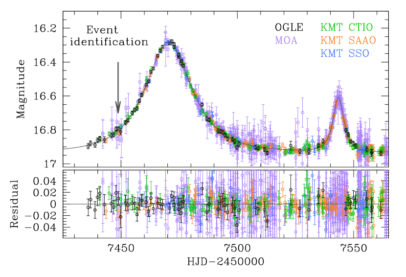
Figure 1.— Light curve of OGLE-2016-BLG-0263. The curve superposed on the data points represents the best-fit binary-lens model. The arrow denotes the time when the event was first discovered. The lower panel shows the residual from the model.

2. Observation and Data

The low-mass binary companion was discovered from the observation of the microlensing event OGLE-2016-BLG-0263. In Figure 1, we present the light curve of the event. The event occurred on a star located toward the Galactic bulge field with equatorial coordinates $({\rm RA},{\rm DEC})_{\rm J2000}=(17^{\circ}59^{\prime}34^{\prime\prime}\hskip-2.0pt.9,-31^{\rm h}49^{\rm m}07^{\rm s}\hskip-2.0pt.0)$ that are equivalent to the Galactic coordinates $(l,b)=(-0^{\circ}\hskip-2.0pt.95,-4^{\circ}\hskip-2.0pt.06)$. The lensing-induced brightening of the source star was identified on 2016 March 1 (${\rm HJD}^{\prime}={\rm HJD}-2450000=7448.7$) by the Early Warning System of the OGLE survey (Udalski et al., 1994; Udalski, 2003) using the 1.3m Warsaw telescope at the Las Campanas Observatory in Chile. Observations by the OGLE survey were conducted with a $\sim 1$ day cadence, and most images were taken in the standard Cousins $I$ band with occasional observations in the Johnson $V$ band for color measurement. After being identified, the event followed a standard point-source point-lens (PSPL) light curve, peaked at ${\rm HJD}^{\prime}\sim 7470$, and gradually returned to the baseline magnitude of $I\sim 16.9$.

However, after returning to baseline, the source began to brighten again. The anomaly was noticed on 2016 May 30 (${\rm HJD}\sim 7538$) and announced to the microlensing community for possible followup observations although no followup observation was conducted. The anomaly, which continued about 10 days, appears to be an independent PSPL event with a short time scale. The time between the first and second peaks of the light curve is $\sim 73$ days.

The event was also in the footprint of the KMTNet and MOA surveys. The survey utilizes three globally distributed 1.6m telescopes that are located at the Cerro Tololo Interamerican Observatory in Chile (KMTC), the South African Astronomical Observatory in South Africa (KMTS), and the Siding Spring Observatory in Australia (KMTA). Similar to OGLE observations, most of the KMTNet data were acquired using the standard Cousins $I$-band filter with occasional $V$-band observations. The event was in the BLG34 field for which observations were carried out with a $\sim 2.5$ hr cadence. The MOA survey uses the 1.6 m telescope located at the Mt. John University Observatory in New Zealand. Data were acquired in a customized $R$ band filter with a bandwidth corresponding to the sum of the Cousin $R$ and $I$ bands. The event was independently found by the MOA survey and was dubbed MOA-2016-BLG-075.

Table 1Error bar correction factors

Data set	$k$	$\sigma_{\rm min}$
OGLE	1.452	0.001
MOA	1.212	0.001
KMT (CTIO)	1.204	0.001
KMT (SAAO)	1.806	0.001
KMT (SSO)	1.300	0.001

Photometry of the images was conducted using pipelines based on the Difference Imaging Analysis method (Alard & Lupton, 1998; Woźniak, 2000) and customized by the individual groups: Udalski (2003) for the OGLE, Albrow et al. (2009) for the KMTNet, and (Bond et al., 2001) for the MOA groups. In order to analyze the data sets acquired by different instruments and reduced by different photometry pipelines, we readjust error bars of the individual data sets. Following the usual procedure described in Yee et al. (2012), we normalize the error bars by

$$\sigma=k(\sigma_{0}^{2}+\sigma_{\rm min}^{2})^{1/2},$$ (1)

where $\sigma_{0}$ is the error bar estimated from the photometry pipeline, $\sigma_{\rm min}$ is a term used to adjust error bars to be consistent with the scatter of the data set, and $k$ is a normalization factor used to make the $\chi^{2}$ per degree of freedom unity. The $\chi^{2}$ value is computed based on the best-fit solution of the lensing parameters obtained from modeling (Section 3). In Table 1, we list the error-bar adjustment factors for the individual data sets. We note that the OGLE data used in our analysis were rereduced for optimal photometry and error bars were estimated according to the prescription described in Skowron et al. (2016), although one still needs a non-unity ($k\neq 1$) scaling factor to make $\chi^{2}/{\rm dof}=1$.

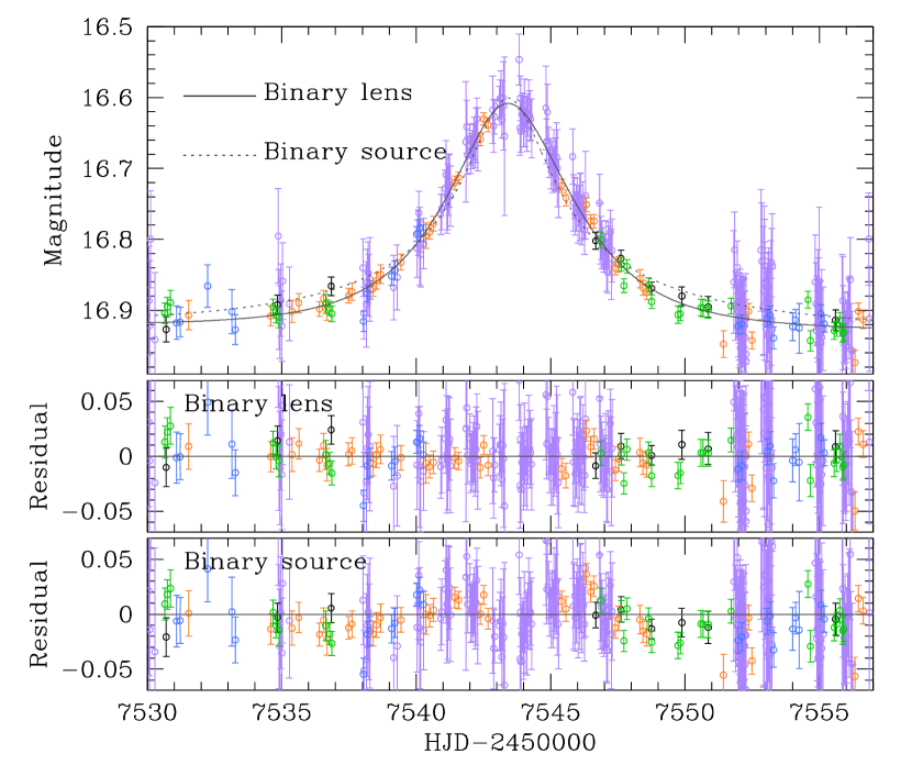
Figure 2.— Enlarged view of the light curve around the second peak. Superposed on the data points are the model light curves obtained from binary-lens (solid) and binary-source (dotted) analysis. The lower panels show the residual from the individual models.

3. Analysis

The light curve of OGLE-2016-BLG-0263 is characterized by two peaks in which the short second one occurred well after the first one. The light curve of such a repeating event can be produced in two cases. The first case is a binary-source event in which the double peaks are produced when the lens passes close to both components of the source separately, one after another (Griest & Hu, 1992; Sazhin & Cherepashchuk, 1994; Han & Gould, 1997). The other case is a binary-lens event where the source approaches both components of a widely separated binary lens, and the source flux is successively magnified by the individual lens components (Di Stefano & Mao, 1996). The degeneracy between binary-source and binary-lens perturbations was first discussed by Gaudi (1998). In order to investigate the nature of the second peak, we test both the binary-source and binary-lens interpretations.

3.1. Binary-Source Interpretation

The light curve of a repeating binary-source event is represented by the superposition of the PSPL light curves involved with the individual source stars, i.e.

$$A_{\rm BS}={A_{1}F_{0,1}+A_{2}F_{0,2}\over F_{0,1}+F_{0,2}}={A_{1}+A_{2}q_{F}\over 1+q_{F}}.$$ (2)

Here $F_{0,i}$ represents the baseline fluxes of the individual source components and $q_{F}=F_{0,2}/F_{0,1}$ is the flux ratio between the source components. The lensing magnification involved with each source component is represented by

$$A_{i}={u_{i}^{2}+2\over u_{i}(u_{i}^{2}+4)^{1/2}};\qquad u_{i}=\left[u_{0,i}^{2}+\left({t-t_{0,i}\over t_{\rm E}}\right)^{2}\right]^{1/2},$$ (3)

where $t_{0,i}$ is the time of the closest lens-source approach, $u_{0,i}$ is the lens-source separation at that moment, and $t_{\rm E}$ is the Einstein time scale. For the basic description of the light curve of a binary-source event, therefore, one needs 6 lensing parameters including $t_{0,1}$, $t_{0,2}$, $u_{0,1}$, $u_{0,2}$, $t_{\rm E}$, and $q_{F}$ (Hwang et al., 2013). The light curve is then modeled as

$$F_{j}(t_{k})=F_{s,j}A_{\rm BS}(t_{k};t_{0,1},u_{0,1},t_{0,2},u_{0,2},t_{\rm E},q_{F}),+F_{b,j},$$ (4)

where the $(F_{s,j},F_{b,j})$ are specified separately for each observatory but there is a single $q_{F}$ for all observatories using a single band (e.g., $I$ band).

We model the observed light curve based on the binary-source parameters. Since the light curve of a binary-source event varies smoothly with the changes of the lensing parameters, we search for the best-fit parameters by $\chi^{2}$ minimization using a downhill approach. For the downhill approach, we use the Markov Chain Monte Carlo (MCMC) method. We set the initial values of $t_{0,1}$ and $t_{0,2}$ based on the times of the first and second peaks, respectively, while the initial values of $u_{0,1}$ and $u_{0,2}$ are determined based on the peak magnifications of the individual peaks. Since both PSPL curves of the individual peaks share a common time scale, we set the initial value of $t_{\rm E}$ as the one estimated based on the PSPL fitting of the light curve with the first peak. The initial value of the flux ratio $q_{F}$ is guessed based on the values of $u_{0,i}$.

Table 2Best-fit binary-source solution

Parameter	Value
$\chi^{2}$	2598.8
$t_{0,1}$ (HJD)	2457470.441 $\pm$ 0.028
$t_{0,2}$ (HJD)	2457543.426 $\pm$ 0.028
$u_{0,1}$	0.646 $\pm$ 0.032
$u_{0,2}$	0.095 $\pm$ 0.004
$t_{\rm E}$ (days)	15.33 $\pm$ 0.50
$q_{F,I}$	0.037 $\pm$ 0.002
$q_{F,R}$	0.036 $\pm$ 0.002
$F_{s}/F_{b}$	2.452/0.219

In Table 2, we present the parameters of the best-fit binary-source solution. Also presented is the ratio of the source flux $F_{s}$ to that of the blend $F_{b}$ that are estimated from the OGLE data set. The uncertainties of the lensing parameters are estimated based on the scatter of points on the MCMC chain. According to the solution, the second peak was produced by the lens approaching very close to the second source which is approximately 30 times fainter than the primary source star. In Figure 2, we also present the model light curve (dotted curve) superposed on the observed data points. At first glance, the model appears to describe the overall shape of the second peak. However, careful inspection of the model light curve and the residual reveals that the fit is inadequate not only in the rising and falling parts but also near the peak part of the light curve.

We check whether the fit can be further improved with higher-order effects. The trajectory of the lens with respect to the source might deviate from rectilinear due to the orbital motion of the Earth around the sun. We check this so-called ‘microlens-parallax’ effect (Gould, 1992) by conducting additional modeling. Accounting for microlens-parallax effects requires to include 2 additional parameters of $\pi_{{\rm E},N}$ and $\pi_{{\rm E},E}$, which represent the components of the microlens parallax vector $\mbox{\boldmath$\pi$}_{\rm E}$ projected onto the sky along the north and east equatorial coordinates, respectively. The direction of $\mbox{\boldmath$\pi$}_{\rm E}$ corresponds to that of the relative lens-source motion in the Earth’s frame. The magnitude of $\mbox{\boldmath$\pi$}_{\rm E}$ is $\pi_{\rm E}=\pi_{\rm rel}/\theta_{\rm E}$, where $\pi_{\rm rel}={\rm au}(D_{\rm S}^{-1}-D_{\rm L}^{-1})$ is the relative lens-source parallax and $D_{\rm{}_{L}}$ and $D_{\rm S}$ represent the distances to the lens and source, respectively. From the modeling with parallax effects, we find that the improvement of the fit is very minor with $\Delta\chi^{2}\sim 4.4$.

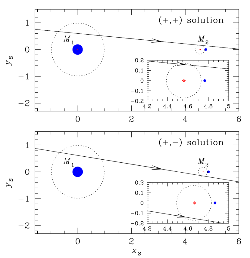
Figure 3.— Lens system geometry that shows the source trajectory (line with an arrow) with respect to the binary-lens components (blue dots). $M_{1}$ and $M_{2}$ denote the heavier and lower-mass components of the binary lens. The dotted circles represent the boundary of effective lensing magnification and the size of each circle corresponds to the Einstein radius corresponding to the mass of each lens component. The tiny close curves at the centers of the dotted circles represent the caustics. The inset shows the enlarged view of the caustic located close to $M_{2}$.

3.2. Binary-Lens Interpretation

Unlike the case of a binary-source event, the light curve of a binary-lens event cannot be described by the superposition of the two light curves involved with the individual lens components because the lens binarity induces a region of discontinuous lensing magnifications, i.e. caustics. As a result, the lensing parameters needed to describe a binary-lens event is different from those of a binary-source event. Basic description of a binary-lens event requires 7 principal parameters. The first three of these parameters, $t_{0}$, $u_{0}$, and $t_{\rm E}$, are the same as those of a single-lens event. The other three parameters describe the binary lens including the projected separation $s$ (normalized to $\theta_{\rm E}$) and the mass ratio $q$ between the binary components, and the angle between the source trajectory and the binary axis, $\alpha$. Light curves produced by binary lenses are often identified by characteristic spike features that are produced by the source crossings over or approaches close to caustics. In this case, the caustic-involved parts of the light curve are affected by finite-source effects. To account for finite-source effects, one needs an additional parameter $\rho=\theta_{*}/\theta_{\rm E}$, where $\theta_{*}$ is the angular source radius. For OGLE-2016-BLG-0263, however, the light curve does not show any feature involved with a caustic and thus we do not include $\rho$ as a parameter.

Binary lenses form caustics of 3 topologies (Schneider & Weiss, 1986; Erdl & Schneider, 1993), which are usually referred to as ‘close’, ‘resonant’, and ‘wide’. For a ‘resonant’ binary, where the projected binary separation is equivalent to the angular Einstein radius, i.e. $s\sim 1$, the caustics form a single big closed curve with 6 cusps. For a ‘close’ binary with $s<1-3q^{1/2}/4$ (Dominik, 1999), the caustic consists of two parts, where one four-cusp caustic is located around the barycenter of the binary lens and two small three-cusp caustics are positioned away from the barycenter. For a ‘wide’ topology with $s>1+3q^{1/2}/2$ (Dominik, 1999), there exist two four-cusp caustics which are located close to the individual lens components.

A repeating binary-lens event is produced by a wide binary lens, and the individual peaks of the repeating event occur when the source approaches the four-cusp caustics of the wide binary lens. The caustic has an offset of $\Delta x\sim q/{s(1+q)}$ with respect to each lens position toward the other lens component (Di Stefano & Mao, 1996; An & Han, 2002). In the very wide binary regime with $s\gg 1$, each of the two caustics is approximated by the tiny astroidal Chang-Refsdal caustic with an external shear $\gamma=q/[s^{2}(1+q)]$ (Chang & Refsdal, 1984) and the offset $\Delta x\rightarrow 0$, implying that the position of the caustic approaches that of the lens components. In this regime, the light curves involved with the individual binary-lens components are described by two separate PSPL curves, and the light curve of the repeating event is approximated by the superposition of the two PSPL curves, i.e. $F_{\rm obs}(t)=F_{S}[A_{1}(t)+A_{2}(t)]+F_{b}$, where $F_{\rm obs}$ is the observed flux and $A_{1}$ and $A_{2}$ represent the lensing magnifications involved with the individual lens components. To be noted is that the time scales of the two PSPL curves of a repeating event are proportional to the square root of the masses of the lens components, i.e. $t_{{\rm E},2}/t_{{\rm E},1}=(m_{2}/m_{1})^{1/2}=q^{1/2}$, while the time scales of the two PSPL curves of a repeating binary-source event are the same because both PSPL curves are produced by a common lens.

To test the binary-lens interpretation, we conduct binary-lens modeling of the observed light curve. Similar to the binary-source case, we set the initial values of the lensing parameters based on the time of the major peak for $t_{0}$, the peak magnification of the major event for $u_{0}$, the duration of the major event for $t_{\rm E}$, the ratio of the time gap between the two peaks to the event time scale for $s\sim\Delta t/t_{\rm E}$, the ratio between the time scales of the first and second events for $q\sim(t_{{\rm E},2}/t_{{\rm E},1})^{2}$, and $\alpha\sim 0$ for a repeating binary-lens event. Based on these initial values, we search for a binary-lens solution using the MCMC downhill approach. To double check the result, we conduct a grid search for a solution in the parameter space of $(s,q,\alpha)$. From this, we confirm that the solution found based on the initial values of the lensing parameters converges to the solution found by the grid search.

Although the binary-lensing model does not suffer from the degeneracy in the $s$ and $q$ parameters, it is found that there exists a degeneracy in the source trajectory angle $\alpha$. This degeneracy occurs because a pair of solutions with source trajectories passing the lens components on the same, (+,+) solution, and the opposite, (+,-) solution, sides with respect to the binary axis result in similar light curves. See Figure 3. For OGLE-2016-BLG-0263, we find that the (+,+) solution is slightly preferred over the (+,-) solution by $\Delta\chi^{2}=7.8$.

Table 3Best-fit binary-lens solution

Parameter	(+,+) solution	(+,-) solution
$\chi^{2}$	2438.2	2446.0
$t_{0}$ (HJD)	2457470.433 $\pm$ 0.036	2457470.432 $\pm$ 0.036
$u_{0}$	0.581 $\pm$ 0.027	0.599 $\pm$ 0.031
$t_{\rm E}$ (days)	16.24 $\pm$ 0.45	15.92 $\pm$ 0.51
$s$	4.72 $\pm$ 0.12	4.86 $\pm$ 0.15
$q$ ($10^{-2}$)	3.06 $\pm$ 0.08	2.97 $\pm$ 0.09
$\alpha$ (radian)	0.095 $\pm$ 0.002	0.163 $\pm$ 0.003
$F_{s}/F_{b}$	2.419/0.254	2.543/0.131

In Table 3, we present the best-fit binary-lens parameters along with the $\chi^{2}$ value of the fit. Since the degeneracy between (+,+) and (+,-) solutions is quite severe, we present both solutions. Because the difference between the source trajectory angles of the two solutions is small, it is found that the lensing parameters of the two solutions are similar to each other. Two factors to be noted are first the binary separation, $s\sim 4.7$, is substantially greater than the Einstein radius and second the mass ratio between the lens components, $q\sim 0.03$, is quite small. We present the model light curve of the best-fit binary-lens solution, i.e. (+,+) solution, in Figure 1 for the whole event and in Figure 2 for the second peak.

In Figure 3, we present the lens system geometry that shows the source trajectory (line with an arrow) with respect to the lens components (marked by blue dots). The upper and lower panels are for the (+,+) and (+,-) solutions, respectively. The tiny red cuspy closed curves near the individual lens components represent the caustics. We note that all lengths are scaled to the angular Einstein radius corresponding to the total mass of the binary lens. The two dotted circles around the individual caustics represent the Einstein rings corresponding to the masses of the individual binary-lens components with radii $r_{1}=[1/(1+q)]^{1/2}$ and $r_{2}=[q/(1+q)]^{1/2}$. From the geometry, one finds that the source trajectory approached both lens components and the two peaks in the lensing light curve were produced at the moments when the source approached the caustics near the individual lens components. In the regime with a small mass ratio, $q\ll 1$, the caustics located close to the higher and lower-mass lens components are often referred to as ‘central’ and ‘planetary’ caustics, respectively. The small central caustic is located very close to the higher-mass lens component and its size as measured by the width along the binary axis is $\sim 4q/(s-s^{-1})^{2}\sim 0.006$ (Chung et al., 2005). The comparatively larger planetary caustic is located on the side of the lower-mass lens component with a separation from the heavier lens component of $\sim s-1/s\sim 4.6$. The size of the planetary caustic is related to the separation and mass ratio of the binary lens by $\sim 4q^{1/2}/[s(s^{2}-1)^{1/2}]\sim 0.03$ (Han, 2006). Since the distance to each caustic from the source trajectory is much greater than the caustic size, the light curve involved with each lens component appears as a PSPL curves.

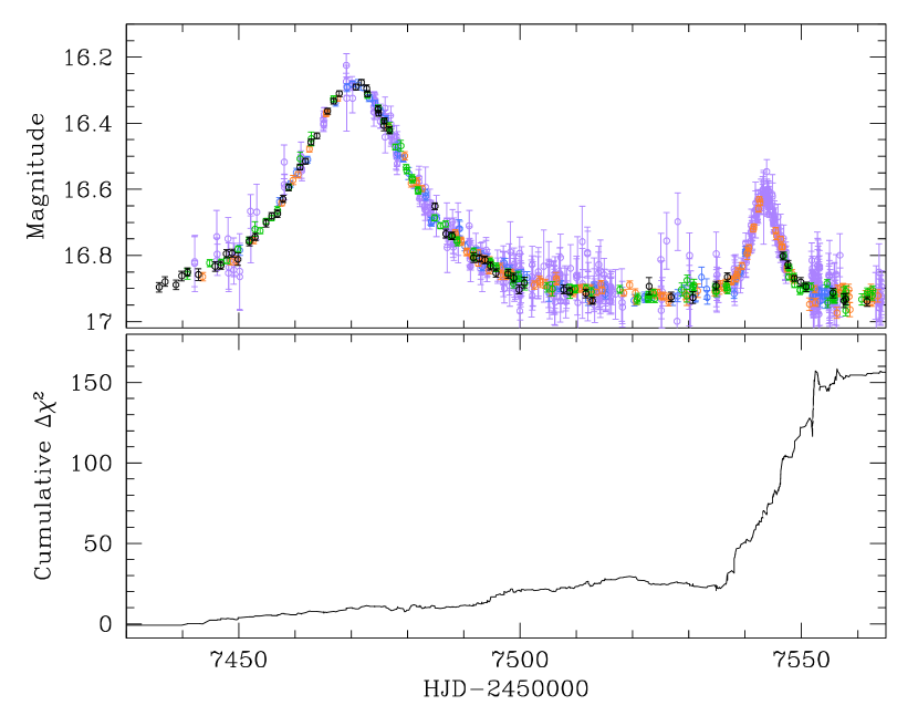
Figure 4.— Cumulative distribution of $\Delta\chi^{2}=\chi_{\rm BS}^{2}-\chi_{\rm BL}^{2}$, where $\chi_{\rm BS}^{2}$ and $\chi_{\rm BL}^{2}$ represent the $\chi^{2}$ values of the binary-source and binary-lens models, respectively.

3.3. Comparison of Models

Knowing that both binary-source (BS) and binary-lens (BL) interpretations can explain the repeating nature of the lensing light curve, we compare the two models in order to find the correct interpretation of the event. For this, we construct the cumulative distribution of $\chi^{2}$ difference between the two models.

Figure 4 shows the constructed $\Delta\chi^{2}$ distribution where $\Delta\chi^{2}=\chi_{\rm BS}^{2}-\chi_{\rm BL}^{2}$. The distribution shows that the binary-lens interpretation better describes the observed light curve than the binary-source interpretation does. The biggest $\Delta\chi^{2}$ occurs during the second peak. This can be seen also in Figure 2, where the residuals from both models around the second peaks are presented. The total $\chi^{2}$ difference is $\Delta\chi^{2}\sim 160$. To show the statistical significance of the difference between the two models, we conduct a $F$-test for the residuals from the models in the region around the second peak. From this, we find $F=1.78$. This corresponds to a $\sim 96\%$ probability that the two models have different variances, suggesting that the models can be distinguished with a significant confidence level.

We note that the unambiguous discrimination between the two interpretations was possible due to the continuous coverage of the second peak using the globally distributed telescopes. One may note large gaps in the observations from Chile ($7537<{\rm HJD}^{\prime}<7546$) and Australia ($7540<{\rm HJD}^{\prime}<7551$), which were both due to bad weather. Nevertheless, the anomaly was continuously covered by the KMTS and MOA data, enabling accurate interpretation of the event.

Another way to discriminate the binary-source/binary-lens interpretations is to use color information. This is possible because the color measured during the two peaks would be different for the binary-source interpretation while the colors should be the same for the binary-lens interpretation. According to the small flux ratio presented in Table 2, the stellar types of the source stars would be greatly different. If a binary-source interpretation is correct, then, the source stars should have significantly different colors. The second peak was observed in $V$ band by the MOA and KMTNet surveys. In Figure 5, we present the $V$-band data plotted over the $I$ and $R$-band data, showing that the second peak was covered in $V$ band with 6 and 2 points by the MOA and KMTNet surveys, respectively. In the binary-source modeling, we introduce two flux ratios $q_{F,I}$ and $q_{F,R}$ to check the possibility of measuring the color difference between the source stars, i.e. $\Delta(R-I)=(R-I)_{1}-(R-I)_{2}=2.5\log(q_{F,I}/q_{F,R})$. We note that the $R$-band flux ratio is measured based on the MOA data. From this, we find $q_{F,I}=0.037\pm 0.02$ and $q_{F,R}=0.036\pm 0.02$, indicating no color change within the error bar. This suggests the inconsistency in the binary-source interpretation and further supports the binary-lens interpretation.

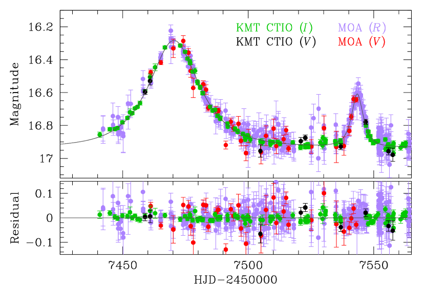
Figure 5.— $V$-band data from the MOA and KMTNet surveys.

3.4. Source Star

Characterizing the source star of a lensing event is important for caustic-crossing binary-lens events because the angular source radius $\theta_{*}$ combined with the normalized source radius $\rho$ enables one to determine the angular Einstein radius, i.e. $\theta_{\rm E}=\theta_{*}/\rho$. Although one cannot determine $\theta_{\rm E}$ for OGLE-2016-BLG-0263 because the source did not cross caustics and thus the light curve is not affected by finite-source effects, we characterize the source star for the sake of completeness.

The source star is characterized based on its de-reddened color $(V-I)_{0}$ and brightness $I_{0}$. We determine $(V-I)_{0}$ and $I_{0}$ of the source star using the usual method of Yoo et al. (2004), where the instrumental color and brightness of the source are calibrated using the position of the giant clump (GC) centroid, for which the de-reddened color and brightness $(V-I,I)_{0,{\rm GC}}=(1.06,14.63)$ (Bensby et al., 2011; Nataf et al., 2013) are known.

Figure 6 shows the position of the source star with respect to the GC centroid in the instrumental color-magnitude diagram of stars in the $205"\times 205"$ image stamp centered at the source position. The locations of the source and GC centroid are $(V-I)=(-0.07,15.89)$ and $(V-I)_{\rm GC}=(0.07,14.70)$, respectively. From the offsets in color $\Delta(V-I)=(V-I)-(V-I)_{\rm GC}=-0.14$ and magnitude $\Delta I=I-I_{\rm GC}=1.19$, we estimate that the re-reddened color and magnitude of the source star are $(V-I,I)_{0}=(0.99,15.82)$. This indicates that the source is a K-type giant star.

Figure 6.— Position of the source star with respect to the centroid of giant clump in the instrumental color-magnitude diagram of stars in the neighboring region around the source.

3.5. Physical Parameters

For the unique determination of the mass $M$ and distance $D_{\rm L}$ to the lens, one needs to measure both the microlens parallax $\pi_{\rm E}$ and the angular Einstein radius $\theta_{\rm E}$ that are related to $M$ and $D_{\rm L}$ by

$$M={\theta_{\rm E}\over\kappa\pi_{\rm E}};\qquad D_{\rm L}={{\rm au}\over\pi_{\rm E}\theta_{\rm E}+\pi_{\rm S}},$$ (5)

where $\kappa\equiv 4G/(c^{2}\ {\rm au})\simeq 8.144\ {\rm mas}\ M_{\odot}^{-1}$ and $\pi_{\rm S}$ denotes the source parallax. For OGLE-2016-BLG-0263, none of these quantities is measured and thus the physical parameters cannot be uniquely determined. However, one can still statistically constrain the physical lens parameters based on the measured event time scale $t_{\rm E}$ that is related to the physical parameters by

$$t_{\rm E}={(\kappa M\pi_{\rm rel})^{1/2}\over\mu};\qquad\pi_{\rm rel}={\rm au}\left({1\over D_{\rm L}}-{1\over D_{\rm S}}\right),$$ (6)

where $\mu$ represents the relative lens-source proper motion.

In order to estimate the mass and distance to the lens, we conduct a Bayesian analysis of the event based on the measured event time scale combined with the mass function of lens objects and the models of the physical and dynamical distributions of objects in the Galaxy. We use the initial mass function of Chabrier (2003a) for the mass function of Galactic bulge objects, while we use the present day mass function of Chabrier (2003b) for disk object. We note that the adopted mass functions extend to substellar objects down to $0.01\ M_{\odot}$.

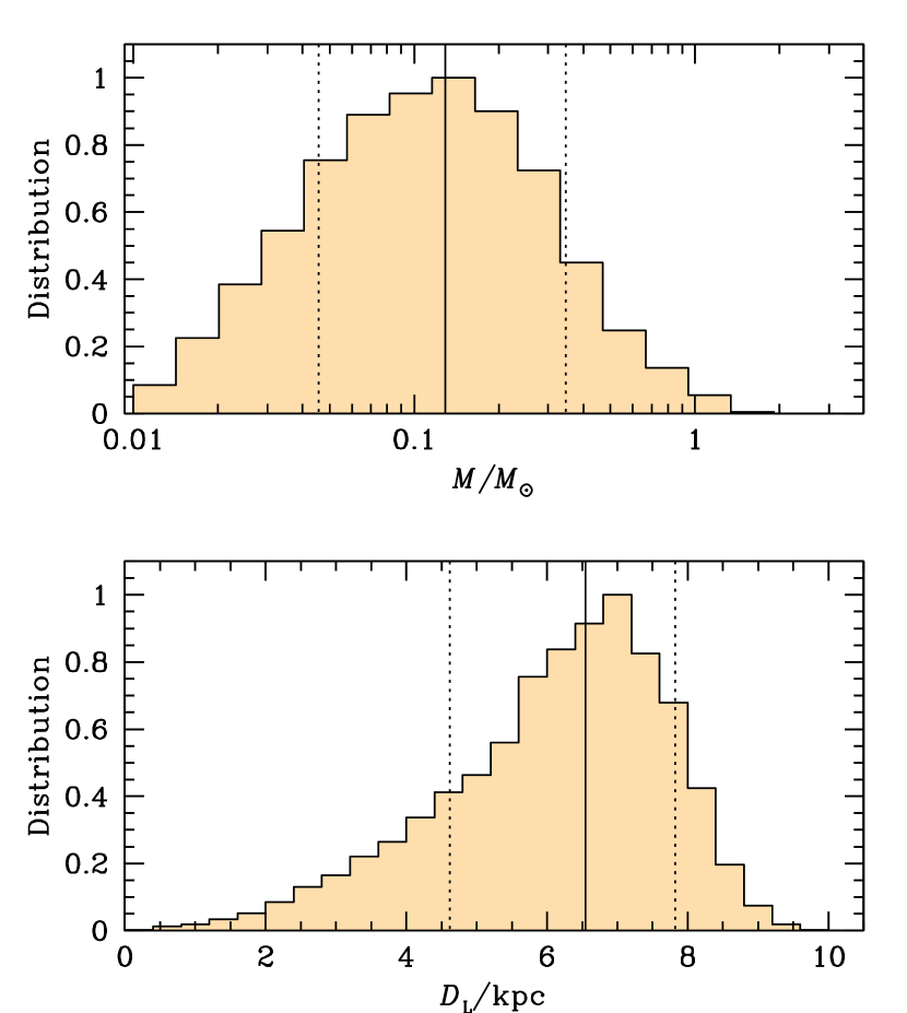
Figure 7.— Distributions of the lens mass (upper panel) and the distance to the lens (lower panel) estimated by Bayesian analysis. The solid vertical line in each panel denotes the median value and the region surrounded by the dotted lines represents 1$\sigma$ (68%) range of the distribution.

Table 4Physical parameters

Parameter	Value
Mass of the primary ($M_{1}$)	$0.13^{+0.21}_{-0.08}$ $M_{\odot}$
Mass of the companion ($M_{2}$)	$4.1^{+6.5}_{-2.5}$ $M_{\rm J}$
Distance to the lens ($D_{\rm L}$)	$6.5^{+1.3}_{-1.9}$ kpc
Projected separation ($a_{\perp}$)	$5.4^{+1.1}_{-1.6}$ au

For the matter density distribution, we adopt the Galactic model of Han & Gould (2003), where the matter density distribution is constructed based on a double-exponential disk and a triaxial bulge. The velocity distribution is constructed based on the Han & Gould (1995) model, where the disk velocity distribution is assumed to be Gaussian about the rotation velocity of the disk and the bulge velocity distribution is modeled to be a triaxial Gaussian with velocity components deduced from the flattening of the bulge via the tensor virial theorem. Based on the models, we generate a large number of artificial events by conducting a Monte Carlo simulation. We then estimate the ranges of $M$ and $D_{\rm L}$ corresponding to the measured event time scale.

In Figure 7, we present the probability distributions of the lens mass (upper panel) and distance to the lens (lower panel) obtained from the Bayesian analysis. In Table 4, we also present the estimated masses of the individual lens components, $M_{1}$ and $M_{2}$, the distance to the lens, $D_{\rm L}$, and the projected separation between the lens component, $a_{\perp}$. We choose the median values of the distributions as representative values and the uncertainties of the physical parameters are estimated based on the upper and lower boundaries within which 68% ($1\sigma$) of the distribution is encompassed.

The estimated mass of the primary lens is $M_{1}=0.13^{+0.21}_{-0.08}\ M_{\odot}$. The central value corresponds to a low-mass M dwarf, which is the most common lens population. The mass of the companion is $M_{2}=4.1^{+6.5}_{-2.5}\ M_{\rm J}$. The upper limit, i.e. $\sim 10.6\ M_{\rm J}$, is below the deuterium-burning limit of $\sim 13\ M_{\rm J}$, indicating that the companion is likely to be a planet. The projected separation between the lens components is $a_{\perp}=5.4^{+1.1}_{-1.6}$ au. Under the assumption that the snow line, which separates regions of rocky planet formation from regions of icy planet formation, scales with the mass of a star (Kennedy & Kenyon, 2008), the snow line of the host star is $a_{\rm sl}=2.7\ {\rm au}(M/M_{\odot})\sim 0.35\ {\rm au}$, where 2.7 au is the snow line in the Solar System (Abe et al., 2000; Rivkin et al., 2002). If the companion is a planet, then the ratio of the $M_{1}$ – $M_{2}$ separation to the snow-line distance of the planetary system is $a_{\perp}/a_{\rm sl}\sim 15.4$. This ratio corresponds to the region beyond Neptune, the outermost planet of the solar system.

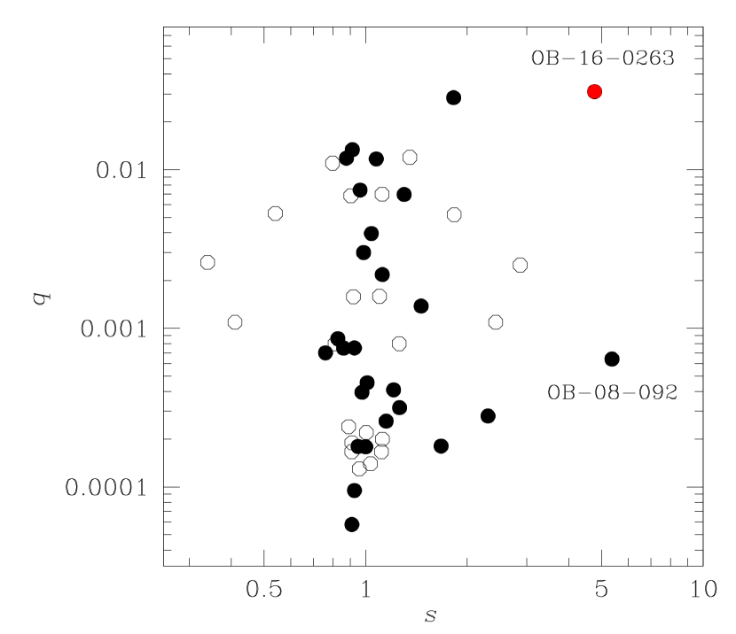
Figure 8.— Plot of planet-star separation $s$ vs. the mass ratio $q$ of 48 previously discovered microlensing planets. The filled dots represent planets for which the lens parameters are uniquely determined, while the empty circles represent planets with close/wide degeneracy. For the planets suffering from the degeneracy, we mark two points with $s$ and $s^{-1}$. The red-filled dot denotes OGLE-2016-BLG-0263Lb reported in this work.

4. Discussion

The discovery of OGLE-2016-BLG-0263LB demonstrates that high-cadence surveys can provide an additional channel of detecting very low-mass companions through repeating events. The scientific importance of the repeating-event channel is that the range of planets and BDs detectable by microlensing is expanded.

The usefulness of the repeating-event channel is illustrated in Figure 8, where we plot the position of OGLE-2016-BLG-0263LB among the 48 previously discovered microlensing planets in the $q$-$s$ parameter space. In the plot, filled circles represent planets for which the lensing parameters are unambiguous determined. On the other hand, empty circles represent planets for which the solutions suffer from degeneracy, mostly by the well-known close/wide degeneracy between the solutions with $s$ and $s^{-1}$ (Griest & Safizadeh, 1998). In this case, we mark both solutions. From the locations of planets, it is found that most planets are concentrated in the region around $s=1.0$ (Mróz et al., 2017) because they were detected from the anomalies that occurred during the lensing magnification by their host stars. By contrast, OGLE-2016-BLG-0263LB is located in the unpopulated region of wide separations. It has the largest separation after OGLE-2008-BLG-092LAb, which had a projected separation from its host of $s\sim 5.3$ (Poleski et al., 2014a). We note that OGLE-2008-BLG-092LAb was also detected through the repeating-event channel.

The repeating-event channel is also important in future space-based microlensing surveys, such as WFIRST, from which many free-floating planet candidates are expected to be detected. Microlensing events produced by free-floating planets appear as short time-scale events. However, bound planets with large separations from their host stars can also produce similar signals, masquerading as free-floating planets (Han et al., 2005). High-cadence ground-based surveys are important because they enable to distinguish some bound planets from free-floating planets through the repeating-event channel. Due to the time-window limit set by the orbits of satellites, space-based lensing observations will not observe the bulge field continuously. For example, the WFIRST survey is planned to be conducted for $\sim 70$ days each season. With the data obtained from space observations, then, it will be difficult to sort out short time-scale events produced by bound planets through the repeating-event channel. On the other hand, ground-based surveys continue for much longer periods, $\sim 8$ months in average, and thus they can provide an important channel to filter out bound planets from the sample of free-floating planet candidates.

Table 5Binary-source solution with two timescales

Parameter	Value
$t_{0,1}$ (HJD)	2457470.465 $\pm$ 0.040
$t_{0,2}$ (HJD)	2457543.474 $\pm$ 0.040
$u_{0,1}$	0.608 $\pm$ 0.049
$u_{0,2}$	0.394 $\pm$ 0.049
$t_{{\rm E},1}$ (days)	15.81 $\pm$ 0.82
$t_{{\rm E},2}$ (days)	5.05 $\pm$ 0.53
$q_{F}$	0.225 $\pm$ 0.026
$F_{s}/F_{b}$	3.098/-0.424

In the usual investigation of binary-source solutions for which the two components are well-separated, these two components are treated as having fixed separation. Hence, in this approximation, the two well-separated events are treated as having a single Einstein time scale $t_{\rm E}$. Indeed, this is one of the principal characteristics used to distinguish binary-source and binary-lens models: if the time scales differ, this implies a binary lens with mass ratio $q=(t_{{\rm E},2}/t_{{\rm E},1})^{2}$.

Nevertheless, at some level, the two components must be moving, so that the Einstein time scales cannot be strictly equal. Here we quantify what level of difference is plausible. Of course it is known that binary orbital motion can give rise to significant light curve variations (Han & Gould, 1997) and these can in principle be quite complicated. However, here we are working in the wide-separation limit and so will take a perturbative approach, defined by

$$\epsilon\equiv{\Delta t_{\rm E}\over t_{\rm E}};\qquad\Delta t_{\rm E}\equiv t_{{\rm E},2}-t_{{\rm E},1}.$$ (1)

Since the components are well-separated, $\Delta t_{\rm E}$ is sensitive only to motion along the direction of projected separation

$$\Delta v_{s,\parallel}=D_{s}(\mu_{s,2,\parallel}-\mu_{s,1,\parallel})=D_{s}\biggl{(}{\theta_{\rm E}\over t_{{\rm E},2}}-{\theta_{\rm E}\over t_{{\rm E},1}}\biggr{)}\simeq-{D_{s}\theta_{\rm E}\Delta t_{\rm E}\over t_{\rm E}^{2}}.$$ (2)

The projected physical separation between the components is

$$a_{\perp}=D_{s}\mu_{\rm rel}\Delta t_{0}=D_{s}\theta_{\rm E}{\Delta t_{0}\over t_{\rm E}};\qquad\Delta t_{0}\equiv t_{0,2}-t_{0,1}$$ (3)

Then, for the system to be bound, $v_{s,\parallel}^{2}<GM_{s}/a_{\perp}$, where $M_{s}$ is the total mass of the source (typically $M_{s}\sim 2\,M_{\odot}$ for two sources visible in the bulge, although this may not hold if one of these repeating events is extremely highly magnified). This can be expressed

$$1>{a_{\perp}v_{s,\parallel}^{2}\over GM_{s}}=\biggl{(}{D_{s}\theta_{\rm E}\over t_{\rm E}}\biggr{)}^{3}{\Delta t_{0}\over GM_{s}}\epsilon^{2},$$ (4)

i.e.,

$${\theta_{\rm E}\over{\rm mas}}<{t_{\rm E}\over D_{s}({\rm AU}/{\rm kpc})}\biggl{(}{GM_{s}\over\epsilon^{2}\Delta t_{0}}\biggr{)}^{1/3}={t_{\rm E}/{\rm yr}\over D_{s}/{\rm kpc}}\biggl{(}{4\pi^{2}M_{s}/M_{\odot}\over\epsilon^{2}\Delta t_{0}/{\rm yr}}\biggr{)}^{1/3}.$$ (5)

We now apply this formalism to the case of OGLE-2016-BLG-0263. We first search for binary-source solutions as in Section 3.1, but with the additional degree of freedom $t_{\rm E}\rightarrow(t_{{\rm E},1},t_{{\rm E},2})$. The results in Table 5 show that this model comes close to matching the binary-lens model in terms of $\chi^{2}$, but at the cost of a radical divergence of Einstein time scales: $(t_{{\rm E},1},t_{{\rm E},2})=(15.8,5.0)\,$days. We note that, in addition, the blending is negative, $F_{b}=-0.42$, which corresponds to an $I=19$ “anti-star”, which would require a “divot” in the stellar background of this amplitude. Negative blending might be caused either by an incorrect model or fluctuation of data for a small $F_{b}$ case. Due to the latter possibility, negative blending at this level cannot be excluded.

To apply the formalism, we first note that the flux of the secondary indicates that it is an upper main sequence star, so that indeed the masses of the two sources are $M_{s,1}\simeq M_{s,2}\simeq 1\,M_{\odot}$. We then adopt $t_{\rm E}=(t_{{\rm E},1}t_{{\rm E},2})^{1/2}=8.9\,$days, so that $\epsilon=1.17$, which is outside the “perturbative regime”. Nevertheless, if one carries through the non-perturbative calculation, the final result hardly differs. We obtain

$$\theta_{\rm E}<0.02\,{\rm mas};\quad\mu<0.8\,{\rm mas\,yr^{-1}}.$$

The limit on $\mu$ would already make the lens quite unusual, though hardly unprecedented. However, the low value of $\theta_{\rm E}$ is more constraining. For example, for typical bulge lenses with $D_{S}-D_{L}=1\,$kpc, this would imply a lens mass $M_{L}<0.003\,M_{\odot}$, and for disk lenses, $M_{L}$ would be even lower. The combination of somewhat low proper motion and very low Einstein radius would make this a very remarkable lens.

Moreover, we note that we have been extraordinarily conservative in putting “1” on the r.h.s of Equation (4). Because we are viewing only one component of motion and very few systems would be seen either face-on or near local escape velocity, we could have chosen a typical value “1/8”, rather than a strict upper limit. Thus a more typical source geometry would yield $\theta_{\rm E}\sim 0.01\,$mas, which would imply $M_{L}<0.0007\,M_{\odot}$,

We conclude that while the data can be well matched to a binary-source with large internal motion, this requires an improbably small Einstein radius. Hence, in this case such solutions are highly disfavored.

References

- Abe et al. (2000) Abe, Y., Ohtani, E., Okuchi, T., Righter, K., & Drake, M. 2000, Origin of the Earth and Moon, eds R. M. Canup, K. Righter, (Tucson: Univ. Ariz. Press), 413
- Alard & Lupton (1998) Alard, C., & Lupton, R. H. 1998, ApJ, 503, 325
- Albrow et al. (2009) Albrow, M. D., Horne, K., Bramich, D. M., et al. 2009, MNRAS, 397, 2099
- An & Han (2002) An, J. H., & Han, C. 2002, ApJ, 573, 351
- Beaulieu et al. (2006) Beaulieu, J.-P., Bennett, D. P., Fouqué, P.; et al. 2006, Nature, 439, 437
- Bensby et al. (2011) Bensby, T., Adén, D., Meléndez, J., et al. 2011, A&A A, 533, 134
- Bond et al. (2001) Bond, I. A., Abe, F., Dodd, R. J., et al. 2001, MNRAS, 327, 868
- Chabrier (2003a) Chabrier, G. 2003a, PASP, 115, 763
- Chabrier (2003b) Chabrier, G. 2003b, ApJ, 586, L133
- Chang & Refsdal (1984) Chang, K., & Refsdal, S. 1984, A&A, 132, 168
- Chung et al. (2005) Chung, S.-J., Han, C., & Park, B.-G. 2005, ApJ, 630, 535
- Di Stefano & Mao (1996) Di Stefano, R., & Mao, S. 1996, ApJ, 457, 93
- Di Stefano & Scalzo (1999) Di Stefano, R., & Scalzo, R. A. 1999, ApJ, 512, 579
- Dominik (1999) Dominik, M. 1999, A&A, 349, 108
- Erdl & Schneider (1993) Erdl, H., & Schneider, P. 1993, A&A, 268, 453
- Gaudi (1998) Gaudi, B. S. 1998, ApJ, 506, 533
- Griest & Hu (1992) Griest, K., & Hu, W. 1992, ApJ, 397, 362
- Griest & Safizadeh (1998) Griest, K., & Safizadeh, N. 1998, ApJ, 500, 37
- Gould (1992) Gould, A. 1992, ApJ, 392, 442
- Gould & Loeb (1992) Gould, A., & Loeb, A. 1992, ApJ, 396, 104
- Han (2006) Han, C. 2006, ApJ, 638, 1080
- Han (2007) Han, C. 2007, ApJ, 670, 1361
- Han et al. (2005) Han, C., Gaudi, B. S., An, J. H., & Gould, A. 2005, ApJ, 618, 962
- Han & Gould (1995) Han, C., & Gould, A. 1995, ApJ, 447, 53
- Han & Gould (1997) Han, C., & Gould, A. 1997, ApJ, 480, 196
- Han & Gould (2003) Han, C., & Gould, A. 2003, ApJ, 592, 172
- Han et al. (2016) Han, C., Udalski, A., Gould, A., et al. 2016, AJ, 152, 95
- Henderson & Shvartzvald (2016) Henderson, C. B. & Shvartzvald, Y. 2016, AJ, 152, 96
- Hwang et al. (2013) Hwang, K.-H., Choi, J.-Y., Bond, I. A., et al. 2013, ApJ, 778, 55
- Kennedy & Kenyon (2008) Kennedy, G. M., & Kenyon, S. J. 2008, ApJ, 673, 502
- Kim et al. (2016) Kim, S.-L., Lee, C.-U., Park, B.-G., et al. 2016, JKAS, 49, 37
- Mróz et al. (2017) Mróz, P., Han, C., Udalski, A., et al. 2017, AJ, 153, 143
- Nataf et al. (2013) Nataf, D. M., Gould, A., Fouqué, P., et al. 2013, ApJ, 769, 88
- Poleski et al. (2014a) Poleski, R., Skowron, J., Udalski, A., et al. 2014a, ApJ, 795, 42
- Poleski et al. (2014b) Poleski, R., Udalski, A., Dong, S., al. 2014b, ApJ, 782, 47
- Rivkin et al. (2002) Rivkin, A. S., Howell, E. S., Vilas, F., & Lebofsky, L. A. 2002, Asteroids III, eds W. K. Bottke, A. Cellino, P. Paolicchi, R. P. Binzel (Tucson: Univ. Ariz. Press), 235
- Sazhin & Cherepashchuk (1994) Sazhin, M. V., & Cherepashchuk, A. M. 1994, Astron. Lett., 20, 523
- Schneider & Weiss (1986) Schneider, P., & Weiss, A. 1986, A&A, 164, 237
- Shin et al. (2016) Shin, I.-G., Ryu, Y.-H., Udalski, A., et al. 2016, Journ. Korean Astro. Soc., 49, 73
- Skowron et al. (2016) Skowron, J., Udalski, A., Kozłowski, S., et al. 2016, Acta Astron., 66, 1
- Sumi et al. (2003) Sumi, T., Abe, F., Bond, I. A., et al. 2003, ApJ, 591, 204
- Udalski (2003) Udalski, A. 2003, Acta Astron., 53, 291
- Udalski et al. (2005) Udalski, A., Jaroszyński, M., Paczyński, B., et al. 2005, ApJ, 628, L109
- Udalski et al. (1994) Udalski, A., Szymański, M., Kałużny, J., Kubiak, M., Mateo, M., Krzemiński, W., & Paczyński, B. 1994, Acta Astron., 44, 227
- Udalski et al. (2015) Udalski, A., Szymański, M. K., & Szymański, G. 2015, Acta Astron., 65, 1
- Woźniak (2000) Woźniak, P. R. 2000, Acta Astron., 50, 421
- Yee et al. (2012) Yee, J. C., Shvartzvald, Y., Gal-Yam, A., et al. 2012, ApJ, 755, 102
- Yoo et al. (2004) Yoo, J., DePoy, D. L., Gal-Yam, A., et al. 2004, ApJ, 603, 139