Density Functional Theory of doped superfluid liquid helium and nanodroplets

Abstract

During the last decade, density function theory (DFT) in its static and dynamic time dependent forms, has emerged as a powerful tool to describe the structure and dynamics of doped liquid helium and droplets. In this review, we summarize the activity carried out in this field within the DFT framework since the publication of the previous review article on this subject [M. Barranco et al., J. Low Temp. Phys. 142, 1 (2006)]. Furthermore, a comprehensive presentation of the actual implementations of helium DFT is given, which have not been discussed in the individual articles or are scattered in the existing literature. This is an Accepted Manuscript of an article published on August 2, 2017 by Taylor & Francis Group in Int. Rev. Phys. Chem. 36, 621 (2017), available online: http://dx.doi.org/10.1080/0144235X.2017.1351672

Contents

page

I. Introduction I
II. Density functional theory of liquid ⁴He at zero temperature II
   II.A. Theoretical basis of density functional theory II.1
   II.B. The Orsay-Trento density functional II.2
   II.C. Recent improvements of the OT-DFT functional II.3
         II.C.1. The ‘solid’ density functional II.3.1
         II.C.2. Instability of the backflow term II.3.2
III. Time-independent calculations III
   III.A. General considerations III.1
   III.B. Introduction of vorticity III.2
IV. Dynamics IV
   IV.A. Heavy impurities IV.1
   IV.B. Test particle method for light impurities IV.2
   IV.C. Simulation of absorption and emission spectra using the density
          fluctuation method IV.3
V. Recent applications of DFT for impurity doped superfluid helium V
   V.A. Alkali metal doped helium droplets: solvation and absorption spectra V.1
   V.B. Alkaline earth metal doped helium droplets: solvation and absorption
          spectra V.2
   V.C. Droplets doped with more than one species V.3
   V.D. Cluster-doped helium droplets V.4
   V.E. Doped mixed ³He-⁴He and ³He droplets V.5
   V.F. Electrons in liquid helium V.6
   V.G. Cations in liquid helium and droplets V.7
   V.H. Intrinsic helium impurities V.8
   V.I. Translational motion of ions below the Landau critical velocity V.9
   V.J. Critical Landau velocity in small ⁴He droplets V.10
   V.K. Rotational superfluidity V.11
   V.L. Interaction of impurities with vortex lines V.12
         V.L.1. Electrons V.12.1
         V.L.2. Atomic and molecular impurities V.12.2
   V.M. Vortex arrays in ⁴He droplets V.13
   V.N. Dynamics of alkali atoms excited on the surface of ⁴He droplets V.14
   V.O. Capture of impurities by ⁴He droplets V.15
         V.P.1. Pure droplets V.15.1
         V.P.2. Droplets hosting vortices V.15.2
   V.Q. Liquid helium on nanostructured surfaces V.16
   V.R. Soft-landing of helium droplets V.17
VI Summary and outlook VI

I Introduction

Liquid helium-4 becomes superfluid below the lambda transition at 2.17 K due to partial Bose-Einstein condensation (BEC). It exhibits unusual macroscopic behavior such as e.g. vanishing viscosity and the thermo-mechanical effect.Til74 On the atomic scale, the response of this fascinating quantum liquid has been studied experimentally by using solvated atomic and molecular species as probes.Bor07 The early experiments employed bulk liquid helium samples where only ionic species and intrinsic helium excimers could be introduced. A breakthrough in this area has been the development of the helium droplet technique, which made it possible to embed neutral atomic and molecular species in superfluid helium droplets at 0.37 K.Har95 ; Har96 In addition to their intrinsic interest as a superfluid object of finite size, helium droplets provide an ideal matrix for spectroscopic experiments due to their low temperature and weak interaction with the solvated species.Leh98 ; Toe04 ; Bar06 ; Sza06 ; Sti06 ; Cho06 ; Tig07 ; Sle08 ; Cal11a ; Yan13 ; Mud14 ; Toe90 ; Wha94 ; Wha98 ; Toe98 ; Nor01 ; Kro02

From the theoretical point of view, superfluid helium must be considered as a high dimensional quantum system. Quantum Monte Carlo (QMC)Kro02 and direct quantum mechanicaldeL06 ; deL10 ; Agu13 calculations are the most accurate methods, but their computational demand quickly exceeds currently available computer resources when the number of helium atoms increases. Furthermore, QMC cannot describe dynamic evolution of superfluid helium in real time. To address these limitations, approximate methods based on density functional theory (DFT) formalism have been introduced.Str87a ; Str87b ; Dal95 DFT can be applied to much larger systems than QMC and allows for time-dependent formulation. As such, it offers a good compromise between accuracy and computational feasibility. The main drawback of DFT is that the exact energy functional is not known and must therefore be constructed in a semi-empirical manner. Nevertheless, DFT is the only method to date that can successfully reproduce results from a wide range of time-resolved experiments in superfluid helium on the atomic scale.

Application of recently developed femtosecond laser techniques to study helium dropletsMud14 ; Zie15 highlights the importance of time-dependent DFT (TDDFT). For example, TDDFT can be used to analyze experiments that employ free electron laser pulses to visualize vortex arrays in helium droplets,Gom14 or the dynamics following optical excitation of guest atoms or molecules embedded in helium droplets.Bra13 ; Van17 It is the only method that allows for such a close interplay between theory and time-resolved helium droplet experiments. In fact, many of the results presented in this review were obtained as joint experimental-theoretical collaborative work.

Despite the wide success of both DFT and TDDFT, they have known limitations, especially when the interaction between the guest species and helium is strong.Lea14b ; Fie12 New strategies for resolving with such problems are also summarised in this review. In addition, applications of DFT and time-dependent DFT will be reviewed with a focus on the new developments that have appeared after the previous review article on this topic.Bar06

We provide a comprehensive presentation of the most recent DFT models and their applications to superfluid helium droplets and bulk liquid. Selected topics dealing with DFT of non-superfluid ³He are also briefly discussed; some practical details of the DFT implementation are given in Ref. dft-guide, . As stated by Frank Stienkemeier and Kevin Lehmann in their 2006 topical review,Sti06 a truly comprehensive review of the activity carried out recently in this field would require a monograph instead of a review article; the reader is thus referred to the appropriate literature, in particular to some recent reviewsToe04 ; Bar06 ; Sza06 ; Sti06 ; Cho06 ; Tig07 ; Sle08 ; Cal11a ; Yan13 ; Mud14 ; Zie15 for the subjects not considered in detail here.

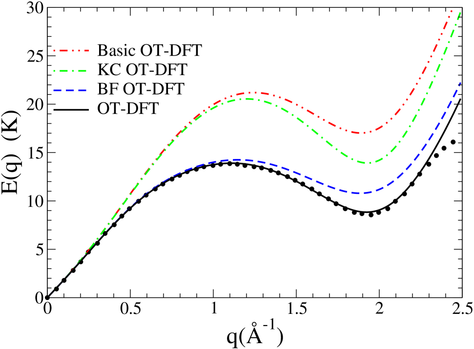
Figure 1: Dispersion relation for elementary excitations in liquid ⁴He calculated as in Ref. Mat10a, . ‘Basic’ indicates the OT-DFT without the non-local kinetic energy correlation (KC) nor the backflow (BF) terms; KC OT-DFT adds to the basic OT-DFT the KC term; BF OT-DFT adds to the basic OT-DFT the BF term. The dots are the experimental data from Ref. Don81, . The Landau velocity $v_{L}=E(q)/(\hbar\,q)|_{min}$ obtained for each functional is 60.3 m/s (OT-DFT); 75.1 m/s (BF OT-DFT); 94.4 m/s (KC OT-DFT); 118 m/s (basic OT-DFT); and 57.5 (experiment).

II Density functional theory of liquid ⁴He at zero temperature

II.1 Theoretical basis of density functional theory

The starting point is the Hohenberg-Kohn (HK) theorem,Hoh64 which states that the total energy $E$ of a many-body quantum system at $T=0$ is a functional of the one-particle density $\rho({\mathbf{r}})=\langle\Phi|\sum_{i}\delta({\mathbf{r}}-{\mathbf{r}}_{i})|\Phi\rangle$ ($\Phi$ being the many-body wave function):

$$E[\rho]={\cal T}[\rho]+\int d{\mathbf{r}}\,{\cal E}[\rho]$$ (1)

where the kinetic energy functional has been separated from the interaction part.

The Kohn-Sham formulationKoh65 of the HK theorem allows to write the above functional in the form

$$E[\rho]=T[\rho]+\int d{\mathbf{r}}\,{\cal E}_{c}[\rho]$$ (2)

where $T[\rho]$ is the kinetic energy of a fictitious system of non-interacting particles, with the same density of the original one, described by single-particle orbitals $\{\phi_{i}({\mathbf{r}})\}$

$$T=-\frac{\hbar^{2}}{2m_{4}}\sum_{i}\int d{\mathbf{r}}\,\phi_{i}^{\ast}({\mathbf{r}})\nabla^{2}\phi_{i}({\mathbf{r}})$$ (3)

The sum extends to the $N_{4}$ particles of mass $m_{4}$ in the system. The difference ${\cal T}[\rho]-T[\rho]$ has been buried in the interaction term ${\cal E}_{c}$. The density of such non-interacting system is thus $\rho({\mathbf{r}})=\sum_{i}|\phi_{i}({\mathbf{r}})|^{2}$. We conform here to the common notation used for DFT studies of helium systems,Dal95 which defines as ‘correlation energy density’ the functional ${\cal E}_{c}$, even if it includes also He-He interactions at the mean-field level (first term in Eq. (8) below).

Assuming complete Bose-Einstein condensation at $T=0$ (i.e. all the ⁴He atoms are in the same single-particle orbital $\phi_{0}$), the many-body wave function is simply

$$\Phi({\mathbf{r}}_{1},{\mathbf{r}}_{2},\cdots{\mathbf{r}}_{N_{4}})=\prod_{i=1}^{i=N_{4}}\phi_{0}({\mathbf{r}}_{i})$$ (4)

while $\rho({\mathbf{r}})=N_{4}|\phi_{0}({\mathbf{r}})|^{2}$. Although the actual condensate fraction of superfluid ⁴He is less than 10%, the available helium density functionals have been devised such that, by starting from a fully condensed state, the interaction term ${\cal E}_{c}$ allows to reproduce the relevant physical properties of liquid helium at $T=0$.

It is customary to define an order parameter $\Psi$ (also called effective wave function) as $\Psi(\textbf{r})=\sqrt{N_{4}}\phi_{0}(\textbf{r})$. The kinetic energy of the condensate is thus

$$T[\rho]=-\frac{\hbar^{2}}{2m_{4}}N_{4}\langle\phi_{0}|\nabla^{2}|\phi_{0}\rangle=\frac{\hbar^{2}}{2m_{4}}\int d{\mathbf{r}}|\nabla\Psi|^{2}$$ (5)

The Runge-Gross theorem extends DFT to describe the time evolution of the system through the time-dependent DFT (TDDFT) formalism.Run84 In this case, functional variation of the associated Lagrangian leads to a time-dependent Euler-Lagrange (EL) equation

$$\imath\hbar\frac{\partial}{\partial t}\Psi({\mathbf{r}},t)=\left\{-\frac{\hbar^{2}}{2m_{4}}\nabla^{2}+\frac{\delta{\cal E}_{c}}{\delta\rho}\right\}\Psi(\textbf{r},t)\equiv{\cal H}\left[\rho\right]\,\Psi(\textbf{r},t)$$ (6)

Given the initial state $\Psi(\textbf{r},0)$, solution of this non-linear equation yields $\Psi\left(\textbf{r},t\right)$ which, in the hydrodynamic picture,Mad27 can be decomposed into liquid density and the associated velocity potential field. For stationary states, $\Psi(\textbf{r},t)=\Psi_{0}(\textbf{r})e^{-\i\mu t/\hbar}$ and Eq. (6) can be cast into a non-linear time-independent EL equation

$$\left\{-\frac{\hbar^{2}}{2m_{4}}\nabla^{2}+\frac{\delta{\cal E}_{c}}{\delta\rho}\right\}\Psi_{0}(\textbf{r})=\mu\Psi_{0}(\textbf{r})$$ (7)

where $\mu$ is the chemical potential. Iterative solution of Eq. (7) determines the particle density $\rho(\textbf{r})=|\Psi_{0}(\textbf{r})|^{2}$ (a similar relationship holds in the time-dependent situation) and hence the total energy of the system.

In its time-independent formulation, DFT is a ground-state theory. However, within the HK theorem, the variational principle is applicable to the lowest state of a given symmetry, which may be different from the true ground state of the system. For example, this can be employed to obtain stationary vortex solutions in helium droplets by DFT. Similarly, minimization of the energy functional in the presence of additional constraints (e.g., fixed total angular momentum) will provide the correct density for the associated excited state. In particular, this technique can be used to produce vortex arrays in helium droplets. However, for general excited states, there is no equivalent HK theorem and TDDFT must be used to model them.

In the case of phenomenological helium DFT, the quality of the results depends on the functional form used. As an example, TDDFT calculation of the dispersion relation for uniform liquid helium (an excited state property) is shown in Fig. 1. The OT-DFT introduced below gives results in agreement, by construction, with the experimental (‘exact’) results. This obviously does not guarantee that the same functional would also give reliable results for inhomogeneous systems. However, based on our experience, these functionals are highly ‘transferable’ to such situations and provide results that are generally in good agreement with experiments.

Approximate representations for the interaction energy density functional ${\cal E}_{c}$, which are capable of describing inhomogeneous ⁴He systems quantitatively, are discussed in the following Section.

II.2 The Orsay-Trento density functional

$\epsilon_{LJ}$ (K)	$\sigma$ (Å)	$h$ (Å)	$c_{2}$ (K Å6)	$c_{3}$ (K Å9)	$\alpha_{s}$ (Å3)
10.22	2.556	2.190323	-2.41186 $\times 10^{4}$	1.85850 $\times 10^{6}$	54.31
$\rho_{0s}$ (Å-3)	$l$ (Å)	$C$ (Hartree)	$\beta$ (Å3)	$\rho_{m}$ (Å-3)	$\gamma_{11}$
0.04	1.	0.1	40.	0.37	-19.7544
$\gamma_{12}$ (Å-2)	$\alpha_{1}$ (Å-2)	$\gamma_{21}$	$\gamma_{22}$ (Å-2)	$\alpha_{2}$ (Å-2)
12.5616	1.023	-0.2395	0.0312	0.14912

Table 1: Model parameters for the OT-DFT and solid functionals.

The first and simplest DFT model for superfluid ⁴He was developed by Stringari and coworkers.Str87a ; Str87b In this approach, ${\cal E}_{c}[\rho]$ consists of a sum of terms that only depend on the local density $\rho({\bf r})$. More recent models include also finite-range and non-local terms, which greatly improve the accuracy of the method, especially when applied to highly inhomogeneous systems.

The most successful approach to date is the finite range, non-local Orsay-Trento DFT model (OT-DFT),Dal95 which has been calibrated to reproduce bulk liquid properties such as the energy per atom, the equilibrium density, the dispersion relation, and the compressibility at $P=T=0$. The OT-DFT energy functional is written as

$${\cal E}_{c}[\rho,\mathbf{v}] = \frac{1}{2}\int{\rm d}{\bf r^{\prime}}\rho({\bf r})V_{LJ}(|{\bf r}-{\bf r^{\prime}}|)\rho({\bf r^{\prime}})$$ (8)

$$+\frac{1}{2}c_{2}\,\rho({\bf r})\left[{\bar{\rho}}({\bf r})\right]^{2}+\frac{1}{3}c_{3}\,\rho({\bf r})\left[{\bar{\rho}}({\bf r})\right]^{3}$$

$$-\frac{\hbar^{2}}{4m_{4}}\alpha_{s}\int{\rm d}{\bf r^{\prime}}F(|{\bf r}-{\bf r^{\prime}}|)\left[1-\frac{{\tilde{\rho}}({\bf r})}{\rho_{0s}}\right]\nabla\rho({\bf r})\cdot\nabla^{\prime}\rho({\bf r^{\prime}})\left[1-\frac{{\tilde{\rho}}({\bf r^{\prime}})}{\rho_{0s}}\right]$$

$$-\frac{m_{4}}{4}\int d\mathbf{r}^{\prime}\,V_{J}(|\mathbf{r}-\mathbf{r}^{\prime}|)\,\rho(\mathbf{r})\,\rho(\mathbf{r}^{\prime})\,[\mathbf{v}(\mathbf{r})-\mathbf{v}(\mathbf{r}^{\prime})]^{2}$$

The first term corresponds to a classical Lennard-Jones interaction between helium atoms, which is truncated at short distances where the correlation effects become important

$$V_{LJ}(r) = 4\epsilon_{LJ}\left[\left(\frac{\sigma}{r}\right)^{12}-\left(\frac{\sigma}{r}\right)^{6}\right]\quad{\rm if}\quad r>h$$ (9)

$$= 0\quad{\rm otherwise}$$

The second line in Eq. (8) accounts for short-range correlation effects. The third line (‘$\alpha_{s}$ term’) is a non-local kinetic energy correction (KC) – which partially accounts for the difference ${\cal T}[\rho]-T[\rho]$ in the interaction term ${\cal E}_{c}$ – and the last term is the backflow (BF) contribution that affects the dynamic response of the functional. Note that the BF term only contributes when the order parameter is a complex valued function (e.g. time-dependent problem or vortex state). The velocity $\mathbf{v}(\mathbf{r})$ is determined from the current

$$\mathbf{j}(\mathbf{r})=-\frac{\imath\hbar}{2m_{4}}[\Psi^{*}(\mathbf{r})\nabla\Psi(\mathbf{r})-\Psi(\mathbf{r})\nabla\Psi^{*}(\mathbf{r})]$$ (10)

as $\mathbf{v}(\mathbf{r})=\mathbf{j}(\mathbf{r})/\rho(\mathbf{r})=\hbar/m_{4}\times{\rm Im}\{\nabla\Psi(\mathbf{r})/\Psi(\mathbf{r})\}$. The two coarse-grained averages of the liquid density, $\bar{\rho}$ and $\tilde{\rho}$, entering into the short-range correlation terms in Eq. (8), are given by

$${\bar{\rho}}({\bf r})=\int{\rm d}{\bf r^{\prime}}\rho({\bf r^{\prime}})w(|{\bf r}-{\bf r^{\prime}}|)$$ (11)

where

$$w(r) = \frac{3}{4\pi h^{3}}\quad{\rm if}\quad r<h$$ (12)

$$= 0\quad{\rm otherwise.}$$

and

$${\tilde{\rho}}({\bf r})=\int{\rm d}{\bf r^{\prime}}\rho({\bf r^{\prime}})F(|{\bf r}-{\bf r^{\prime}}|)$$ (13)

where $F(r)$ is a Gaussian kernel

$$F(r)=\frac{1}{\pi^{3/2}l^{3}}{\rm e}^{-r^{2}/l^{2}}$$ (14)

The function $V_{J}(r)$ presents in the backflow term is defined as

$$V_{J}(r)=(\gamma_{11}+\gamma_{12}\,r^{2})e^{-\alpha_{1}r^{2}}+(\gamma_{21}+\gamma_{22}\,r^{2})e^{-\alpha_{2}r^{2}}$$ (15)

The various parameters entering the OT-DFT functional are specified in Table 1.

While OT-DFT can model the response of superfluid helium very accurately, it is seldom applied to inhomogeneous systems due to its complexity.Anc10 Furthermore, in most time-dependent applications, both the kinetic energy correlation and backflow terms are often neglected because their evaluation is time consuming and they tend to exhibit numerical instabilities, especially for highly inhomogeneous systems. Strategies for overcoming these instabilities are presented in the next section.

The backflow and non-local kinetic energy correlation terms in OT-DFT are required for a quantitative description of the elementary excitation spectrum of superfluid helium. While both terms influence the energetics of the roton minimum, the backflow term has the most important contribution of the two as demonstrated in Fig. 1. Note that the Landau critical velocity predicted by the functional, which determines the onset of bulk dissipative behavior in time-dependent applications, is the slope of a straight line passing through the origin and tangent to the dispersion curve near the roton minimum.Dal95 ; Pop15 The influence of these terms to the description of a vortex line structure is discussed in Ref. Mat15a, , see also Sec. II.3.2 below.

The accuracy of OT-DFT can be further assessed by comparing the obtained density profiles of pure helium droplets against QMC calculations. By way of an example, such a comparison is shown in Fig. 2 for a droplet with $N_{4}=50$. Since DFT should generally work better when the number of particles increases, OT-DFT will retain its accuracy for the typical droplet sizes produced in experiments (a few thousand ⁴He atoms). Even with the kinetic energy correlation term omitted (i.e. $\alpha_{s}=0$), the agreement with QMC remains rather good as demonstrated in Fig. 2.

In contrast to DFT employing local functionals, the performance of finite-range functionals is superior when processes such as atomic/molecular impurity solvation or their spectroscopy is considered (see e.g. Fig. 1 of Ref. Mat13b, ). Any process that requires the correct liquid response on the Ångström-scale must employ a finite range, non-local model. However, in some applications the non-local terms are not very important and it is possible to use the much simpler local functionals. Local density functionals of different complexity have been used to describe static and dynamic properties of pure and doped superfluid helium.Ber01 ; Mat11a ; Jin10a ; Jin10b ; Jin10c Very recently, a zero-range reduction of the OT functional has also been applied to study inelastic scattering of Xe atoms by quantised vortices in superfluid helium.Psh16

The original OT-DFT formulation only applies to superfluid ⁴He at $T=0$. It has been extended up to $T=3$ K by considering the wetting properties of various metals,Anc00 see also Ref. Bib02, ; Jin12, . A non-local extension of the functional has also been introduced for mixed ³He-⁴He systems.Bar97 The latter model has been used recently to study elementary excitations of superfluid ³He-⁴He mixturesMat10a and to study the solvation of OCS in mixed ³He-⁴He droplets.Lea13 Various functionals have also been developed for pure ³He, see e.g. Refs. Her07, ; Her02, and references therein. Finally, we note that a method similar to the one used for superfluid ⁴He has also been used to describe cold dipolar Bose gasesAba10 and para-hydrogen clusters, for which a DFT-based approach is also available.Anc16

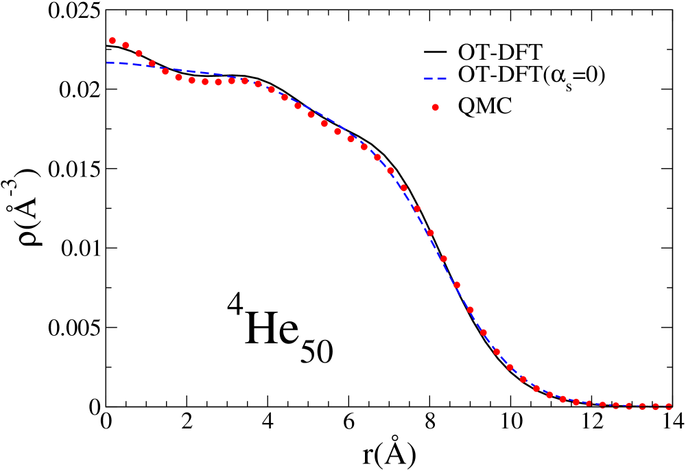
Figure 2: Comparison between OT-DFT and QMC calculations for the density profile of the ⁴He₅₀ droplet. The QMC calculations have been carried out by M. Rossi, University of Padova.

II.3 Recent improvements of the OT-DFT functional

II.3.1 The ‘solid’ density functional

The OT-DFT functional becomes unstable in the presence of highly inhomogeneous liquid density distributions, like those occurring e.g. for the solvation of cations inside ⁴He. To overcome this problem, an additional cutoff term, which was originally developed to account for the liquid-solid phase transition of ⁴He,Anc05a ; Cau07 can be employed to it. This is essentially a penalty term that prevents excessive liquid density accumulation

$${\cal E}_{\rm sol}[\rho(\mathbf{r})]=C\,\rho(\mathbf{r})\{1+\tanh(\beta[\rho(\mathbf{r})-\rho_{\rm m}])\}$$ (16)

Since ${\cal E}_{\rm sol}[\rho]$ is only significant when the liquid density is comparable to $\rho_{\rm m}$ or larger, it does not alter the original OT-DFT functional at densities lower than the (large) cutoff value $\rho_{\rm m}$. For instance, the total energy of pure ⁴He₁₀₀₀ droplet is $-$5400.34 K where the contribution of the penalty term is only 4.2 $\times 10^{-5}$ K. The model parameters used are specified in Table 1.

Inclusion of the ‘solid’ term in the OT-DFT model has made it possible to use it in complex situations where the impurity-helium interaction is strongly attractive. However, while ${\cal E}_{\textnormal{sol}}[\rho]$ in Eq. (16) can prevent the unphysical density pile-up, it cannot eliminate the often observed spontaneous symmetry breaking of the ⁴He order parameter in the presence of strongly attractive external potentials. For instance, the numerical solution can become non-spherical even when the external potential is strictly spherically symmetric. Taking a spherical average of the symmetry broken solution appears however to yield results very close to QMC calculations.Anc07 ; Fie12 It is not clear at the moment how to preserve the desired symmetry during the calculations. Note that a spontaneous symmetry breaking is expected to occur around very attractive impurities, which form ‘snowball’ structures with a solid-like first solvation layer. The solid OT-DFT functional, consisting of ${\cal E}_{\rm sol}$ and the first three terms of Eq. (8), has often been used in the static and dynamic applications discussed in the next sections.

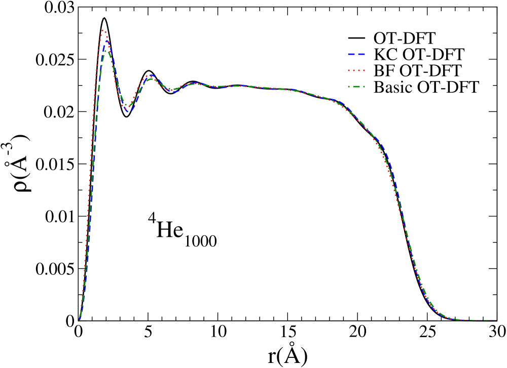
Figure 3: Density profile of the ⁴He₁₀₀₀ droplet hosting a linear vortex along its diameter. As in Fig. 1, the calculations have been carried out using the full OT-DFT or including only some of its terms.

II.3.2 Instability of the backflow term

$P$	$\rho$	$q_{R}$ (exp)	$\Delta$ (exp)	$q_{R}$ (OT)	$\Delta$ (OT)
(bar)	(10-2 Å${}^{-3})$	(Å${}^{-1})$	(K)	(Å${}^{-1})$	(K)
0	2.1836	1.93	8.62	1.92	8.84
5	2.2994	1.97	8.33	1.95	8.52
10	2.3916	2.01	8.03	1.97	8.24
15	2.4694	2.03	7.75	1.99	7.98
20	2.5374	2.06	7.44	2.01	7.73
24	2.5865	2.05	7.30	2.01	7.54
73.2	3.0			2.10	5.48
181.4	3.5			2.21	1.50
195.9	3.55			2.22	0.74
211.2	3.6			-	-

Table 2: OT-DFT zero temperature equation of state $P(\rho)$ of liquid ⁴He and roton minimum parameters calculated by the method of Ref. Mat10a, . The experimental results are from Ref. Gib99, .

The dispersion relation of elementary excitations in liquid ⁴He is shown in Fig 1. The low wavenumber ($q$) region exhibits linear behaviour and corresponds to phonons (sound), followed by a maximum (maxon), and a high-$q$ region that corresponds to collective excitations called rotons. The latter region exhibits a distinct minimum around $q\approx 2$ Å^-1 (roton minimum). Within the previously developed microscopic variational approach of Feynman and Cohen,Fey56 a quantitative description of the roton minimum required the introduction of specific corrections to describe the correlated motion around each atom in the superfluid (backflow).

The formulation of the BF term in OT-DFT,Dal95 which is shown on the fourth line of Eq. (8), was inspired by a previous work of Thouless.Tho69 With this term included, OT-DFT can accurately reproduce the $T=0$ experimental dispersion relation up to the solidification pressureGib99 with the exception of the turn-over region at high momenta beyond the roton region.Don81

The roton minimum can be charaterised by two parameters, $\mu_{R}$ and $q_{R}$, by fitting the experimental dispersion relation close to the minimum with the following function at $T=0.5$ KGib99

$$E(q)=\Delta+\frac{\hbar^{2}}{2\mu_{R}}(q-q_{R})^{2}$$

where $q$ is the wavenumber, $\Delta$ is the roton energy, and $\mu_{R}$ defines the curvature at the roton minimum. A comparison of the experimental $\Delta$ and $q_{R}$ values with those obtained with the OT-DFT functional in shown in Table 2.

The BF term becomes numerically unstable when $\rho\rightarrow 0$ and $\left|\textbf{v}\right|\neq 0$. This instability is present in the energy functional as well as in the corresponding functional derivative yielding the effective potential in Eq. (8).Gia03 ; Leh04 Since the contribution of the BF term should be negligible at low densities, this problem can be eliminated by introducing a density cutoff for evaluating the velocity field from the probability current: $\textbf{v}=\textbf{j}/\left(\rho+\epsilon_{v}\right)$ where $\epsilon_{v}$ is the density cutoff value. Typical values of $\epsilon_{v}$ applied in recent workMat15a are in the order of $7\times 10^{-5}$ Å^-3, which can be compared with the bulk liquid density $\rho_{0}=2.1836\times 10^{-2}$ Å^-3 at $P=T=0$. An alternative approach is to neglect the BF term when the density becomes smaller than a given threshold value (ca. $10^{-6}$ Å^-3).Anc10

Figure 3 shows the density profile for a ⁴He₁₀₀₀ droplet hosting a vortex line, which was calculated by the full OT-DFT or including only some of its term. The BF term reduces the vortex line energy $E_{V}$ by about 20 K. Indeed, by using Eq. (30) and the definition of $E_{V}$ given in Sec. III.2, one finds 127.1 K (basic OT-DFT); 124.2 K (KC OT-DFT); 107.5 (BF OT-DFT), and 105.5 K (OT-DFT).

With the sole exception of electrons,Anc10 all attempts made so far to include the BF term in calculations modelling impurity dynamics in superfluid helium droplets or in bulk liquid have failed. One possible reason for such a failure is the appearance of a dynamic instability: the rationale for this being that the OT-DFT roton minimum energy collapses to zero around densities between 0.0355 and 0.036 Å^-3 as shown in Table 2. Indeed, local liquid densities around impurities which exhibit strong binding towards helium may reach densities much higher than solid helium, leading to an unphysical behavior of the BF term and break down of the OT-DFT model.

It is likely that the BF term should only be applied in the liquid phase for which it was originally intended for. For example, the first solvation layers around snowball structures should be excluded from the BF interaction. A similar remark applies to the KC term, although it has not been found to be unstable. On the other hand, the solvation structures of electrons and vortices are free from such huge density pile-ups and the OT-DFT functional can be employed.Anc10

The instability of the backflow term appearing at high densities calls for improvements. We present here a modified BF term that is numerically stable, only acts in the liquid phase and, by construction, yields a functional of the same quality as the original oneDal95 in that physical region.

Consider a BF term of the following form

$${\cal H}_{BF}=-\frac{m_{4}}{4}\int\int d\mathbf{r}\,d\mathbf{r}^{\prime}\,V_{J}(|\mathbf{r}-\mathbf{r}^{\prime}|)\,G(\rho(\mathbf{r}))\,G(\rho(\mathbf{r}^{\prime}))\,\rho(\mathbf{r})\,\rho(\mathbf{r}^{\prime})\,[\mathbf{v}(\mathbf{r})-\mathbf{v}(\mathbf{r}^{\prime})]^{2}$$ (17)

If one takes

$$G(\rho(\mathbf{r}))=[1-\Theta(\rho(\mathbf{r})-\rho_{BF})]$$

with $\rho_{BF}=0.033$ Å^-3 and $\Theta(x)=1$ if $x\geq 0$ and zero otherwise, this will make the BF contribution effective only when helium is a ‘true’ liquid. The function $G(\rho(\mathbf{r}))$ is difficult to handle numerically. In practice, it has been substituted by

$$G(\rho(\mathbf{r}))=\frac{1}{2}\big{\{}1-\tanh[\xi(\rho(\mathbf{r})-\rho_{BF})]\big{\}}$$ (18)

with a sufficiently large value of $\xi$ to make it steep at $\rho(\mathbf{r})\sim\rho_{BF}$. Values used in the calculations are $\xi=10^{4}$ ų and $\rho_{BF}=0.033$ Å^-3.

The contribution of ${\cal H}_{BF}$ to the mean field, applied to the effective wave function $\Psi(\mathbf{r})$, is

$$-\frac{m_{4}}{2}\left[\left.\rho(\mathbf{r})\frac{dG}{d\rho}\right|_{\rho(\mathbf{r})}+G(\rho(\mathbf{r}))\right]\left\{\int d\mathbf{r}^{\prime}\,V_{J}(|\mathbf{r}-\mathbf{r}^{\prime}|)\,\rho(\mathbf{r}^{\prime})\,G(\rho(\mathbf{r}^{\prime}))[\mathbf{v}(\mathbf{r})-\mathbf{v}(\mathbf{r}^{\prime})]^{2}\right\}\Psi(\mathbf{r})$$

$$+\frac{\imath\hbar}{2}\frac{1}{\rho(\mathbf{r})}\nabla_{\mathbf{r}}\cdot\left\{\int d\mathbf{r}^{\prime}\,V_{J}(|\mathbf{r}-\mathbf{r}^{\prime}|)\,\rho(\mathbf{r})\,G(\rho(\mathbf{r}))\,\rho(\mathbf{r}^{\prime})\,G(\rho(\mathbf{r}^{\prime}))[\mathbf{v}(\mathbf{r})-\mathbf{v}(\mathbf{r}^{\prime})]\right\}\Psi(\mathbf{r})$$ (19)

Putting $G(\rho(\mathbf{r}))=1$ reduces it to the OT-DFT expression.Gia03 ; Leh04 Eq. (19) is as complex to use as the original OT-DFT form. The modified OT-DFT functional (MOT-DFT), that includes the solid and modified BF terms, has been tested in dynamic calculations where OT-DFT was unstable; at variance, MOT-DFT has been found to be stable.

Having solved the instability problem in practice, let us mention that it is unclear what is the actual relevance of the BF term – and KC term – for most items addressed in this review. Processes such as photoexcitation and photoionisation of impurities usually involve high liquid densities and velocities in their first stages, which can lead to the production of shock waves, cavitation, and vorticity. None of them are very sensitive to the accurate description of the roton minimum and therefore the contribution of the BF term should be minimal (except for vorticity, for which we have already estimated the error if it is not included in the calculations). It is only after most of the excess energy has been dispersed into the fluid that the proper description of the elementary excitations becomes important, and the OT-DFT model can be applied at that point.

Last but not least, even if its systematic use might be computationally prohibitive, the stable MOT-DFT may be useful to carry out test calculations to calibrate simpler DFT approaches.

III Time-independent calculations

In this section, we describe how to solve the time-independent EL equation, Eq. (7), to obtain the energetics and structure of solvated impurities in superfluid helium. For example, it can be used to determine absorption and emission spectra of atoms/molecules embedded in helium droplets. It also provides a starting point for subsequent time-dependent calculations.

III.1 General considerations

The ground state liquid density of a system can be obtained by solving Eq. (7). This is most often achieved by employing the imaginary time-method (ITM).Leh07b Normalization of the solution to a fixed number of helium atoms in the droplet, $N_{4}$, determines the corresponding chemical potential $\mu$. On the other hand, for the bulk liquid $\mu$ is dictated by the liquid equation of state, which can be obtained from ${\cal E}_{c}$.Pi07 Provided that a sufficiently large volume of liquid is considered, the value of the bulk chemical potential also applies to systems with solvated impurities or free surfaces.

Impurities much heavier than helium can be described classically as point-like particles, providing an external field for the helium density. In contrast, light impurities have to be modelled quantum mechanically based on the Schrödinger equation. In both cases, the impurity-He atom interaction, $V_{X}$, must be known: it is used to construct the impurity-liquid interaction using the pairwise sum approximation. For classical impurities, this interaction is included as an external field in the energy functional, $E\left[\rho\right]$, by integrating over the liquid density

$$E[\rho]\rightarrow E[\rho]+\int d{\mathbf{r}}\rho({\mathbf{r}})V_{X}(|{\mathbf{r}}-{\mathbf{r}}_{I}|)$$ (20)

where ${\mathbf{r}}_{I}$ is the location of the impurity. Eq. (7) is then written as

$$\left\{-\frac{\hbar^{2}}{2m_{4}}\nabla^{2}+\frac{\delta{\cal E}_{c}}{\delta\rho}+V_{X}(|{\mathbf{r}}-{\mathbf{r}}_{I}|)\right\}\Psi({\mathbf{r}})=\mu\Psi({\mathbf{r}})$$ (21)

For impurities requiring quantum mechanical treatment, $E[\rho]$ must also take into account their zero point motion

$$E[\rho]\rightarrow E[\rho]+\frac{\hbar^{2}}{2m_{I}}\int d{\mathbf{r}}_{I}|\nabla_{I}\phi({\mathbf{r}}_{I})|^{2}+\int\int d{\mathbf{r}}d{\mathbf{r}}_{I}\rho({\mathbf{r}})V_{X}(|{\mathbf{r}}-{\mathbf{r}}_{I}|)|\phi({\mathbf{r}}_{I})|^{2}$$ (22)

where $\phi({\mathbf{r}}_{I})$ is the impurity wave function and $m_{I}$ its mass. This yields two coupled equations, one for the liquid and another for the impurity

$$\left\{-\frac{\hbar^{2}}{2m_{4}}\nabla^{2}+\frac{\delta{\cal E}_{c}}{\delta\rho}+\int d{\mathbf{r}}_{I}V_{X}(|{\mathbf{r}}-{\mathbf{r}}_{I}|)|\phi({\mathbf{r}}_{I})|^{2}\right\}\Psi({\mathbf{r}}) = \mu\Psi({\mathbf{r}})$$

$$\left\{-\frac{\hbar^{2}}{2m_{I}}\nabla^{2}_{I}+\int d{\mathbf{r}}\,V_{X}(|{\mathbf{r}}-{\mathbf{r}}_{I}|)\rho({\mathbf{r}})\right\}\phi({\mathbf{r}}_{I}) = \varepsilon\phi({\mathbf{r}}_{I})$$ (23)

In some applications, it may be necessary to fix the distance between the impurity and the centre of mass (COM) of the droplet. This is the case, e.g., when calculating the energy as a function of that distance allows to determine possible energy barriers hindering the motion of the impurity. This can be achieved by including a constraint term in the energy functional. Assuming that the classical impurity lies along the $z$-axis, the constraint can be introduced as

$$E[\rho]+\int d{\mathbf{r}}\rho({\mathbf{r}})V_{X}(|{\mathbf{r}}-{\mathbf{r}}_{I}|)+\frac{\lambda_{C}}{2}\left({\cal Z}-{\cal Z}_{0}\right)^{2}$$ (24)

where ${\cal Z}$ is the instantaneous distance between the impurity and the COM of the droplet, ${\cal Z}_{0}$ is the corresponding preset constrained distance, and $\lambda_{C}$ is a constant determining the strength of the penalty term. Typical values of $\lambda_{C}$ to ensure that the desired distance is retained within 0.1% accuracy are in the $1000-3000$ K Å^-2 range.

To illustrate how this constraint influences the EL equations when the impurity is treated as a quantum particle, we first define the droplet COM position and the expectation value for the quantum impurity position along the $z$-axis

$$Z_{CM} = \frac{1}{N_{4}}\int d{\mathbf{r}}\,z\,\rho({\mathbf{r}})$$

$$z_{imp} = \int d{\mathbf{r}}_{I}\,z_{I}\,|\phi({\mathbf{r}}_{I})|^{2}$$ (25)

With these definitions, Eqs (23) become

$$\left\{-\frac{\hbar^{2}}{2m_{4}}\nabla^{2}+\frac{\delta{\cal E}_{c}}{\delta\rho}+\int d{\mathbf{r}}_{I}V_{X}(|{\mathbf{r}}-{\mathbf{r}}_{I}|)|\phi({\mathbf{r}}_{I})|^{2}+\lambda_{C}[{\cal Z}-{\cal Z}_{0}]\left(\frac{-z}{N_{4}}\right)\right\}\Psi({\mathbf{r}})=\mu\Psi({\mathbf{r}})$$

$$\left\{-\frac{\hbar^{2}}{2m_{I}}\nabla^{2}_{I}+\int d{\mathbf{r}}\,V_{X}(|{\mathbf{r}}-{\mathbf{r}}_{I}|)\rho({\mathbf{r}})+\lambda_{C}[{\cal Z}-{\cal Z}_{0}]\,z_{I}\,\right\}\phi({\mathbf{r}}_{I})=\varepsilon\phi({\mathbf{r}}_{I})$$ (26)

where ${\cal Z}=z_{imp}-Z_{CM}$. For a classical impurity, the term $\lambda_{C}[{\cal Z}-{\cal Z}_{0}](-z/N_{4})$ has to be added to the left hand side of Eq. (21); in this case $z_{imp}$ is the impurity position.

The DFT equations (21) or (23) can be solved by the ITM in cartesian coordinates.Leh07b Most calculations are carried out in full 3D without taking advantage of possible symmetries in the external potential. Densities, wave functions, differential operators, etc., are represented on discrete equally spaced cartesian grids. The spatial step employed in these calculations is typically ca. 0.4 Å. The differential operators (first and second derivatives) are represented by $k$-point formulas or evaluated directly in the Fourier space using the split operator technique.Leh04 In the former case, 13-point formulas have been found accurate enough.

Since the integral terms in OT-DFT can be expressed as convolutions,Dal95 ; Anc05a ; Leh04 they can be conveniently computed in the Fourier space. Therefore, a key tool for an efficient numerical implementation of OT-DFT is the Fast Fourier Transformation (FFT) technique.Fri05 FFT algorithms are well established in the literature and have efficient parallel implementations. Note that many of the transformations required for evaluating the OT-DFT functional need to be carried out only once.

III.2 Introduction of vorticity

In order to represent a sustained current in liquid helium, the order parameter must be a complex valued function. This is the case for a vortex line, which involves liquid circulation around its core. Vorticity around the symmetry axis ($z$) of an axially symmetric helium droplet can be represented by

$$\Psi(r,\theta)\equiv\rho^{1/2}(r)\,e^{\imath m\theta}$$ (27)

where $r$ is the distance from the symmetry axis, $\theta$ the polar angle, and $m$ the circulation quantum number. This is an eigenfunction of the total angular momentum operator, $\hat{L}_{z}\Psi(r,\theta)=mN_{4}\hbar\Psi(r,\theta)$. In practice, only configurations with circulation $m=\pm 1$ are relevant. This is because the kinetic energy of a vortex line is proportional to $m^{2}$ and therefore a vortex line with $m=\pm 2$ is energetically less favored than two separate vortex lines with $m=\pm 1$. A single vortex line in a pure ⁴He₅₀₀ droplet, in a mixed ⁴He₅₀₀+³He₁₀₀ droplet, and the same systems doped with an HCN molecule can be seen in Fig. 30 of Ref. Bar06, .

The EL equations are as for vortex-free droplets, Eqs. (6) and (21), but the effective wave function has to be complex valued. Since the ITM can only converge to a solution that has overlap with the initial order parameter, starting the calculation with an initial guess similar to Eq. (27) will automatically yield the vortex solution. For instance, a vortex line along the $z$ axis can be produced by starting the imaginary-time calculation with the following initial order parameter

$$\Psi(\mathbf{r})=\frac{\rho_{0}^{1/2}(\mathbf{r})}{\sqrt{x^{2}+y^{2}}}\,(x+\imath y)$$ (28)

where $\rho_{0}(\mathbf{r})$ is the density corresponding to either a pure or doped droplet without vortex. In cylindrical coordinates, this expression reduces to Eq. (27) with $m=1$ provided that the density is axially symmetric. For a more detailed discussion, see e.g. Ref. Pi07, .

The energetics of pure and doped helium hosting vortices are usually characterised by the following quantities Pi07 ; Anc15 ; Dal00 ; Mat15a

$\bullet$ Solvation energy of the impurity $X$: $S_{X}=E(X@^{4}{\rm He}_{N})-E(^{4}{\rm He}_{N})$

$\bullet$ Vortex energy: $E_{V}=E(V@^{4}{\rm He}_{N})-E(^{4}{\rm He}_{N})$

$\bullet$ Binding energy of the impurity $X$ to the vortex:

$$B_{X}=S_{X}-\{E[(X+V)@^{4}{\rm He}_{N}]-E(V@^{4}{\rm He}_{N})\}$$

The binding energy is the result of a delicate balance between the contributing terms and the resulting values are typically rather small. For example, the binding energy of a Xe atom to a vortex line is only 3–5 K.Anc14 ; Dal00

The kinetic energy of the superfluid flow in the volume excluded by the impurity intuitively corresponds to $B_{X}$ and for this reason it is also called ‘substitution energy’.Don91 Using a classical sharp wall model for the impurity bubble and vortex line, the binding energy can be approximated asDon91

$$B_{X}=2\pi\frac{\hbar^{2}}{m_{4}}\rho_{0}\,R_{X}\,\left\{\left(1+\frac{a^{2}}{R_{X}^{2}}\right)^{1/2}\,ln\left[\frac{R_{X}}{a}+\sqrt{\left(\frac{R_{X}}{a}\right)^{2}+1}\right]-1\right\}$$ (29)

where $a$ is the radius of the vortex core and $R_{X}$ the radius of the atomic bubble. Using the Xe atom as an example, setting the liquid density to the $T=P=0$ value $\rho_{0}=0.0218$ Å^-3, $a=1$ Å, and the bubble radius to the value where the Xe-He pair potential becomes repulsive, $R_{X}=3.5$ Å, Eq. (29) yields a binding energy $B_{X}=6.1$ K.

The critical angular velocity for nucleating the vortex line represented by Eqs. (27) or (28) in a droplet consisting of $N_{4}$ helium atoms is given byDal96

$$\omega_{c}=\frac{1}{\hbar}\,\frac{E_{V}}{N_{4}}$$ (30)

where $E_{V}$ is the vortex energy as defined above. For a ⁴He₁₀₀₀ droplet this gives $\omega_{c}=0.127\,{\rm K}/\hbar=0.0166\,{\rm ps}^{-1}$.

The above approach can be used to create individual vortex lines. A different strategy has to be employed to generate an array of vortex lines. A rotational constraint is imposed in the rotating frame of reference (‘co-rotating frame’) by solving the following EL equation

$$[{\cal H}-\omega\hat{L}_{z}]\,\Psi(\mathbf{r})=\,\mu\,\Psi(\mathbf{r})\;,$$ (31)

where $\cal{H}$ is the DFT Hamiltonian (Eq. (6)), $\hat{L}_{z}$ is the $z$-component of the angular momentum operator, and $\omega$ is the angular velocity of the co-rotating frame.

Note that for a vortex array $\Psi(\mathbf{r})$ is no longer an eigenvector of the angular momentum.

The initial guess for imaginary-time evolution can be obtained by the ‘imprinting’ method; for $n_{v}$ vortex lines, the initial guess $\Psi(\mathbf{r})$ is written as

$$\Psi(\mathbf{r})=\rho_{0}^{1/2}(\mathbf{r})\,\prod_{j=1}^{n_{v}}\left[{(x-x_{j})+\imath(y-y_{j})\over\sqrt{(x-x_{j})^{2}+(y-y_{j})^{2}}}\right]$$ (32)

where $\rho_{0}(\mathbf{r})$ is the density of the vortex-free droplet and $(x_{j},y_{j})$ is the initial position of the $j$^th linear vortex core parallel to the $z$-axis. Note that the expression for $\Psi(\mathbf{r})$ was incorrectly written in Refs. Anc14, ; Anc15, . During the imaginary-time relaxation, the positions of the vortex lines will change until convergence to the lowest energy configuration for a given $\omega$ is reached. Complex configurations hosting several vortex lines (vortex arrays) will be described in Sec. V.13.

IV Dynamics

Given a static initial configuration $\Psi(\textbf{r})$ and a known additional perturbation to drive the system, its dynamic evolution can be followed in real-time. The additional perturbation can be, for instance, a sudden photoionisation or photoexcitation of the impurity. As discussed above, a classical or quantum description is employed to propagate the impurity degrees of freedom, depending on its mass as compared to a helium atom.

IV.1 Heavy impurities

Heavy impurities with no evolution in their electronic degrees of freedom can be treated using classical mechanics. Examples include photoexcitation of heavy alkali metal atoms (e.g. Rb, Cs) from the $n$s electronic ground state to the $(n+1)$s excited stateVan14 and photoionisation of a Ba atomMat14 (see also Ref. Lea14b, ) in helium droplets. Typically, these photoexcitation and photoionisation processes are considered to be instantaneous, which means that the light pulse is short enough that the nuclei do not have time to move, but is long enough that its energy spread covers only one (excited or ionised) electronic state.

After ionisation or electronic excitation, the total energy of the system is written as

$$E[\Psi,\mathbf{r}_{I}]=\int d\mathbf{r}\,\frac{\hbar^{2}}{2m_{4}}|\nabla\Psi|^{2}+\frac{p^{2}_{I}}{2m_{I}}+\int d\mathbf{r}\,{\cal E}_{c}(\rho)+\int d\mathbf{r}\,\rho(\mathbf{r})\,V_{X^{*}}(|\mathbf{r}-\mathbf{r}_{I}|)$$ (33)

where $I$ denotes the impurity and $V_{X^{*}}$ is the $X$-He pair potential for the excited or ionised state. $V_{X^{*}}$ (and $V_{X}$ in Sec. III.1) are usually obtained from high-level ab initio calculationsKry08 or accurate semi-empirical methods. Since helium mostly interacts with other species through weak van der Waals forces, accurate treatment of electron correlation is very important.

The time evolution of the helium order parameter $\Psi(\textbf{r},t)$ and the impurity position $r_{I}(t)$ can be obtained from the TDDFT and Newton equations, respectively

$$i\hbar\frac{\partial}{\partial t}\Psi = \left[-\frac{\hbar^{2}}{2m_{4}}\nabla^{2}+\frac{\delta{\cal E}_{c}}{\delta\rho}+V_{X^{*}}(|\mathbf{r}-\mathbf{r}_{I}|)\right]\Psi$$

$$m_{I}\ddot{\mathbf{r}}_{I} = -\nabla_{\mathbf{r}_{I}}\left[\int d\mathbf{r}\,\rho(\mathbf{r})V_{X^{*}}(|\mathbf{r}-\mathbf{r}_{I}|)\right]=-\int d\mathbf{r}\,V_{X^{*}}(|\mathbf{r}-\mathbf{r}_{I}|)\,\nabla\rho(\mathbf{r})\;$$ (34)

For a light impurity (i.e. quantum mechanical treatment), Eqs. (33) and (34) become

$$E[\Psi,\phi] = \int d\mathbf{r}\,\frac{\hbar^{2}}{2m_{4}}|\nabla\Psi|^{2}+\int d\mathbf{r}_{I}\,\frac{\hbar^{2}}{2m_{I}}|\nabla_{\mathbf{r}_{I}}\phi|^{2}+\int d\mathbf{r}\,{\cal E}_{c}(\rho)$$ (35)

$$+ \int\int d\mathbf{r}\,d\mathbf{r}_{I}\,\rho(\mathbf{r},t)\,V_{X^{*}}(|\mathbf{r}-\mathbf{r}_{I}|)|\phi(\mathbf{r}_{I},t)|^{2}$$

and

$$i\hbar\frac{\partial}{\partial t}\Psi(\mathbf{r},t)=\left[-\frac{\hbar^{2}}{2m_{4}}\nabla^{2}+\frac{\delta{\cal E}_{c}}{\delta\rho}+\int\,d\mathbf{r}_{I}\,V_{X^{*}}(|\mathbf{r}-\mathbf{r}_{I}|)|\phi(\mathbf{r}_{I},t)|^{2}\right]\Psi(\mathbf{r},t)$$

$$i\hbar\frac{\partial}{\partial t}\phi(\mathbf{r}_{I},t)=\left[-\frac{\hbar^{2}}{2m_{I}}\nabla^{2}_{I}+\int\,d\mathbf{r}\,V_{X^{*}}(|\mathbf{r}-\mathbf{r}_{I}|)\rho(\mathbf{r},t)\,\right]\phi(\mathbf{r}_{I},t)$$ (36)

where $\phi(\mathbf{r}_{I},t)$ is the wave function for the impurity. Since the dynamics of the impurity and that of the liquid tend to have very different time scales, the overall time step has to be chosen with care. A safe choice of the shorter one for both equations can, however, increase the computational time significantly. Using sub-steps for the faster component can in part alleviate such issues. Another problem can arise from the spatial grids. Unless interpolation techniques are employed, both the impurity and the liquid grids must have the same size and step length. Since light impurities are usually fast and therefore require fine grids, this also increases the computational time required for the liquid. An elegant way out of this problem is to propagate the impurity using the so-called ‘test particle’ method.Wya05 This approach has been used to simulate the Na and Li atom dynamics in helium droplets following the $(n+1)$s $\leftarrow$ $n$s excitation.Her12a

A more complicated situation is encountered when the impurity electronic degrees of freedom must also be included in the dynamics. For example, when an impurity is excited from a spherical $n$s to a $n^{\prime}$p state, the three degenerate p states are split by the dynamic Jahn-Teller effect. The interaction between a He atom and the $L=1$ state impurity can be decomposed into $\Sigma$ ($\Lambda=0$) and a doubly degenerate $\Pi$ ($\Lambda=\pm 1$) state, where $\Lambda$ is the projection of the orbital angular momentum on the interatomic axis. So far, only the case where the impurity can be treated classically has been considered.Mat13b To account for the dynamic orientation of the p-orbital, a simple diatomics-in-molecules (DIM) model can be applied.Ell63 ; Her08a ; Elo01b Its basic ingredients are given below.

The electronic structure of a $n^{\prime}$p-state impurity (i.e. effective one-electron excited ²P atomic state) interacting with He atoms can be expressed in an effective one-electron p-orbital basis. In the diatomic frame coinciding with the $n^{\rm th}$ helium atom (¹S) along the $z_{n}$-axis, the minimal DIM basis set is $|p_{xn}\rangle$, $|p_{yn}\rangle$, $|p_{zn}\rangle$, and the helium-impurity interaction is given by

$$U(r_{n})=V_{\Pi}(r_{n})\mathbf{I}+\{V_{\Sigma}(r_{n})-V_{\Pi}(r_{n})\}|p_{zn}\rangle\langle p_{zn}|$$ (37)

where $r_{n}$ is the interatomic distance and $V_{\Pi}(r)$ and $V_{\Sigma}(r)$ are the $\Pi$ and $\Sigma$ impurity-He pair potentials in the absence of spin-orbit coupling.

For a system consisting of $N_{4}$ helium atoms and an excited p-state impurity, the total potential energy is constructed using the DIM modelEll63

$$U=\sum_{n=1}^{N_{4}}\left\{V_{\Pi}(r_{n})\mathbf{I}+[V_{\Sigma}(r_{n})-V_{\Pi}(r_{n})]R_{n}|p_{z}\rangle\langle p_{z}|R^{-1}_{n}\right\}$$ (38)

where $R_{n}$ is a rotation matrix which transforms the common laboratory frame to the diatomic frame corresponding to the $n^{\rm th}$ He atom. In cartesian coordinates

$$\langle p_{i}|R_{n}|p_{z}\rangle\langle p_{z}|R^{-1}_{n}|p_{j}\rangle=\frac{r_{in}~{}r_{jn}}{r_{n}^{2}}$$ (39)

where $r_{1n}\equiv x_{n}$, $r_{2n}\equiv y_{n}$, $r_{3n}\equiv z_{n}$, and $r_{n}^{2}=x_{n}^{2}+y_{n}^{2}+z_{n}^{2}$ for the $n^{\rm th}$ He atom. The matrix elements of the DIM Hamiltonian are then

$$\langle p_{i}|U|p_{j}\rangle\equiv U_{ij}=\sum_{n=1}^{N_{4}}\left\{V_{\Pi}(r_{n})\delta_{ij}+[V_{\Sigma}(r_{n})-V_{\Pi}(r_{n})]\frac{r_{in}~{}r_{jn}}{r_{n}^{2}}\right\}$$ (40)

Since DFT provides a continuous distribution, the discrete sum over helium atoms is replaced by integration over the density ($\sum_{n}\rightarrow\int\mathrm{d}^{3}\mathbf{r^{\prime\prime}}\rho(\mathbf{r^{\prime\prime}})$), which gives

$$U_{ij}(\mathbf{r})=\int\mathrm{d}^{3}\mathbf{r^{\prime}}\rho(\mathbf{r^{\prime}}+\mathbf{r})\left\{V_{\Pi}(r^{\prime})\delta_{ij}+[V_{\Sigma}(r^{\prime})-V_{\Pi}(r^{\prime})]\frac{r^{\prime}_{i}~{}r^{\prime}_{j}}{r^{\prime 2}}\right\}$$ (41)

The eigenvalues $V^{\mathrm{ex}}_{m}(\mathbf{r})$ of this real symmetric matrix define the potential energy curves (PEC) as a function of the distance between the surrounding helium and the impurity.

The above model assumes that spin-orbit (SO) coupling is negligible. However, when it becomes comparable to the helium induced splitting of the p-orbitals, it must be included in the calculation. The total Hamiltonian is then given by $U_{T}=U+U_{SO}$ where $U_{SO}$ is the SO hamiltonian matrix, usually approximated by that of the free atom.Jak97 The previously mentioned minimal DIM basis set can be extended to include the electron spin: $s=\uparrow(m_{s}=$ ${}^{1}\!/_{2})$, $s=\downarrow(m_{s}=-^{1}\!/_{2})$, i.e. $|i,s\rangle\equiv|p_{x},\uparrow\rangle,|p_{x},\downarrow\rangle,|p_{y},\uparrow\rangle,|p_{y},\downarrow\rangle,|p_{z},\uparrow\rangle,|p_{z},\downarrow\rangle$.

Kramers’ theorem states that the two-fold degeneracy of the levels originating from total half-integer spin cannot be broken by electrostatic interactions.Nak01 Thus, all the electronic eigenstates of $U_{T}$ are doubly degenerate. Diagonalization of $U_{T}$ yields three doubly degenerate PEC between the impurity and surrounding helium. This method has also been extended to impurities in D electronic states.Lea16 ; Mel14

The DIM wave function of the impurity, $|\lambda\rangle$, is determined by a six-dimensional state vector

$$|\lambda\rangle=\sum_{\mathop{i=x,y,z}\limits_{s=-1/2,1/2}}\lambda_{is}|i,s\rangle\;\;.$$ (42)

The complete set of variables required to describe the system consists of the complex valued effective wave function for helium $\Psi(\mathbf{r},t)$ with $\rho(\mathbf{r},t)=|\Psi(\mathbf{r},t)|^{2}$, the impurity position $\mathbf{r}_{I}(t)$, and the 6-dimensional complex vector to determine its electronic wave function $|\lambda(t)\rangle$. The total energy of the impurity-⁴He_N complex after excitation to the ²P manifold is

$$E[\Psi,\mathbf{r}_{I},\lambda]=\int d\mathbf{r}\,\frac{\hbar^{2}}{2m}|\nabla\Psi|^{2}+\frac{p^{2}_{I}}{2m_{I}}+\int d\mathbf{r}\,{\cal E}_{c}[\rho]+\langle\lambda|V_{SO}|\lambda\rangle+\int d\mathbf{r}\,\rho(\mathbf{r})\,V_{\lambda}(\mathbf{r}-\mathbf{r}_{I})$$ (43)

where $V_{SO}$ is the spin-orbit coupling operator and $V_{\lambda}$ is defined as

$$V_{\lambda}(\mathbf{r})\equiv\langle\lambda|{\mathcal{V}}(\mathbf{r})|\lambda\rangle=\sum_{ijss^{\prime}}\lambda^{*}_{is}{\mathcal{V}}^{ijss^{\prime}}(\mathbf{r})\lambda_{js^{\prime}}$$ (44)

with the components of the six-dimensional matrix ${\mathcal{V}}$ given by

$${\mathcal{V}}^{ijss^{\prime}}(\mathbf{r})=\left[V_{\Pi}(r)\delta_{ij}+\left(V_{\Sigma}(r)-V_{\Pi}(r)\right)\frac{r_{i}r_{j}}{r^{2}}\right]\delta_{ss^{\prime}}$$ (45)

The time evolution of the system is obtained by minimizing the action

$${\cal A}[\Psi,\mathbf{r}_{I},\lambda]=\int dt\left\{E[\Psi,\mathbf{r}_{I},\lambda]-i\hbar\int d\mathbf{r}\,\Psi^{*}(\mathbf{r})\frac{\partial}{\partial t}\Psi(\mathbf{r})-i\hbar\langle\lambda|\frac{\partial}{\partial t}|\lambda\rangle-\frac{1}{2}m_{I}\dot{\mathbf{r}}^{2}_{I}\right\}\;$$ (46)

Variation of $\cal A$ with respect to $\Psi^{*}$, $\langle\lambda|$ and $\mathbf{r}_{I}$ yields

$$i\hbar\frac{\partial}{\partial t}\Psi=\left[-\frac{\hbar^{2}}{2m}\nabla^{2}+\frac{\delta{\cal E}_{c}}{\delta\rho(\mathbf{r})}+V_{\lambda}(\mathbf{r}-\mathbf{r}_{I})\right]\Psi$$

$$i\hbar\frac{\partial}{\partial t}|\lambda\rangle={\cal H}\;|\lambda\rangle$$

$$m_{I}\ddot{\mathbf{r}}_{I}=-\nabla_{\mathbf{r}_{I}}\left[\int d\mathbf{r}\rho(\mathbf{r})V_{\lambda}(\mathbf{r}-\mathbf{r}_{I})\right]=-\int d\mathbf{r}\,V_{\lambda}(\mathbf{r}-\mathbf{r}_{I})\nabla\rho(\mathbf{r})$$ (47)

where the explicit time dependence of the variables is omitted for clarity. The second line of Eq. (47) is a $6\times 6$ matrix equation with the matrix elements given by

$$H^{ijss^{\prime}}=\int d\mathbf{r}\,\rho(\mathbf{r}){\mathcal{V}}^{ijss^{\prime}}(\mathbf{r}-\mathbf{r}_{I})+V^{ijss^{\prime}}_{SO}$$ (48)

In order to solve Eqs. (34), (36) or (47), initial values for the variables must be specified. Their choice is guided by the physics of the process studied. The initial helium order parameter and the initial impurity position are usually taken from the static solution of the doped droplet, with the initial impurity velocity set to zero. The initial choice for $|\lambda\rangle$ is dictated by the optical excitation process. It is often taken as one of the eigenstates of the DIM hamiltonian at the time of the electronic excitation.

All dynamic equations in this Section, as e.g. Eq (47), have been solved by using Hamming’s predictor-modifier-corrector method,Ral60 initiated by a fourth-order Runge-Kutta-Gill algorithm.Ral60 ; Pre92 The integration time step employed in most applications is about 0.5 fs.

The time-dependent relaxation of liquid helium around excited state impurities leads to the creation of sound waves and even shock waves when steep repulsive interactions are present. In helium droplets this can also lead to helium evaporation at the droplet surface. Eventually, evaporated helium and bulk liquid excitations will reach the simulation box boundaries and re-enter the box from the opposite side [periodic boundary conditions (PBC) are implied by the use of FFT to compute the convolution integrals in the OT-DFT equations]. This can interfere with the system in an unphysical and unpredictable way, and lead to significant errors in the calculations.

To avoid such artifacts, absorbing boundaries should be implemented by replacing $\imath\longrightarrow\imath+\Lambda(\mathbf{r})$ in the time-dependent OT-DFT equation.Mat11a The attenuation field $\Lambda(\mathbf{r})$ has the form

$$\Lambda(\mathbf{r})=\Lambda_{0}\left[1+\tanh\left(\frac{s-s_{0}}{a}\right)\right],\quad s\equiv|\mathbf{r}|\;.$$ (49)

No attenuation takes place when $s<(s_{0}-2a)$ since $\Lambda(\textbf{r})\ll 1$. The absorbing region has to be large enough to remove all the unwanted effects due to the presence of the PBC. Note that for this method to work for bulk helium, the chemical potential must be included in the external potential during the TDDFT evolution.Mat11a

Finally, we mention that exciplex configurations can also be studied by DFT. The method, which was inspired by the molecular model of Ref. Net05, , is discussed in detail in Ref. Lea16, .

IV.2 Test particle method for light impurities

If the impurity-helium interaction is highly repulsive in the impurity excited state, its velocity can quickly become very large. Inside the droplet this velocity tends to fall below the Landau critical velocity because the kinetic energy is dissipated through efficient coupling to elementary excitations of the liquid. This process is not instantaneousBue16 ; Mat14 and the impurity velocity can remain high during this initial period. Furthermore, in the case of helium droplets velocities may remain high indefinitely if the impurity leaves it. The wave packet for a light impurity with high velocity exhibits rapid spatial and temporal oscillations, which require the use of very fine spatial grids and short time steps. Since these grids must be compatible with the ones used for helium, the computation especially in 3D becomes quickly unaffordable.

To avoid this problem, the impurity degrees of freedom can be described by Bohmian dynamics.Wya05 This approach, which is equivalent to solving the Schrödinger equation, has been tested for the dynamics of excited state Li and Na atoms ejected from the helium droplet surface.Her12a An overview of this method is given below.

The second line in Eq. (36) can effectively be cast into the format of a time-dependent Schrödinger equation (note that the $I$ index to $\mathbf{r}_{I}$ is dropped to simplify the notation)

$$\imath\hbar\frac{\partial}{\partial t}\phi(\mathbf{r},t)=\left[-\frac{\hbar^{2}}{2m}\nabla^{2}+V(\mathbf{r})\,\right]\phi(\mathbf{r},t)\;.$$ (50)

Using the hydrodynamic form suggested by Madelung,Mad27 the complex wave function can be written as

$$\phi(\mathbf{r},t)\equiv\chi(\mathbf{r},t)e^{i{\cal S}(\mathbf{r},t)}$$ (51)

where $\chi\geq 0$ and ${\cal S}$ are both real valued functions.Wya05 While the real and imaginary parts of $\phi$ may oscillate rapidly, the behavior of $\chi$ and ${\cal S}$ is much smoother than $\phi$ as a function of time.Her12a The associated velocity field and the current density are defined as $\mathbf{v}(\textbf{r},t)\equiv(\hbar/m)\nabla{\cal S}$ and $\mathbf{j}(\mathbf{r},t)\equiv\hbar/(2mi)\,[\phi^{*}\nabla\phi-\phi\nabla\phi^{*}]=\chi^{2}\,\mathbf{v}$. Substitution of Eq. (51) into Eq. (50) and equating the real and imaginary parts of the left and right hand side terms in Eq. (50) yields the following – quantum hydrodynamic – equations for $\chi$ and ${\cal S}$:

$$\frac{\partial\chi^{2}}{\partial t} = -\nabla\cdot\mathbf{j}\;\;\;\;\;\;\;\;\;\;\;\;\;\;\;\;\;\;\;\;\;\;\;\;\;\;\;\;\;\;\;{\rm[continuity\;equation]}$$

$$-\hbar\,\frac{{\partial\cal S}}{\partial t} = \frac{1}{2}\,m\mathbf{v}^{2}+{\cal Q}(\mathbf{r},t)+V(\textbf{r})\;\;\;\;\;{\rm[quantum\;Hamilton-Jacobi\;equation]}$$ (52)

where ${\cal Q}$ is the so-called quantum potential (or quantum pressure)

$${\cal Q}(\mathbf{r},t)\equiv-\frac{\hbar^{2}}{2m}\frac{\nabla^{2}\chi}{\chi}$$ (53)

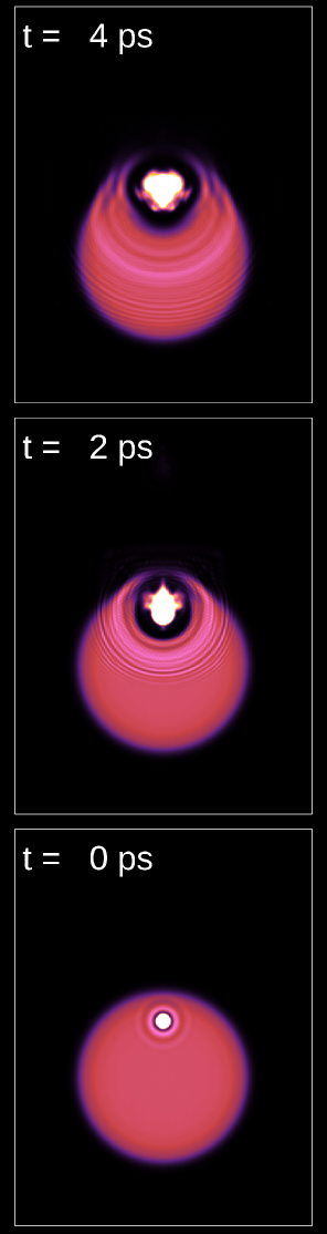
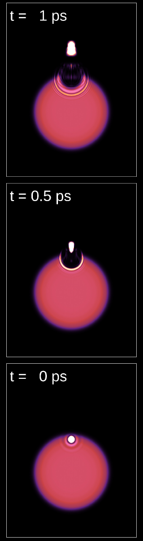
Figure 4: (a) Snapshots of the He density during the evolution of the He^∗@⁴He₁₀₀₀ starting from $\mathbf{r}_{I}$= 15 Å. The bright yellow spot is the probability distribution of the He^∗ being ejected. (b) Same as (a) starting from $\mathbf{r}_{I}$= 20 Å.

The above Eq. (52) can be solved by using the test particle method as follows. The probability density $\chi^{2}$ and the current density as a function of time can be constructed from a histogram based on $M$ test particles. Given a set of test particle trajectories, $\{\mathbf{R}_{i}(t)\}_{i=1}^{M}$, where $\mathbf{R}_{i}(t)=\mathbf{R}(\mathbf{r}_{i},t)$ and $\mathbf{R}_{i}(0)=\mathbf{r}_{i}$, $\chi^{2}$ and $\mathbf{j}$ can be computed as

$$\chi^{2}(\mathbf{r},t) = \lim_{M\rightarrow\infty}\frac{1}{M}\sum_{i=1}^{M}\delta[\mathbf{r}-\mathbf{R}_{i}(t)]$$

$$\mathbf{j}(\mathbf{r},t) = \lim_{M\rightarrow\infty}\frac{1}{M}\sum_{i=1}^{M}\mathbf{v}[\mathbf{R}_{i}(t)]\delta[\mathbf{r}-\mathbf{R}_{i}(t)]\;.$$ (54)

For example, a value of $M=200\,000$ was used in Ref. Her12a, to simulate the desorption of Li and Na atoms excited to the 3s and 4s states, respectively.

The continuity equation is automatically fulfilled provided that $\dot{\mathbf{R}}_{i}(t)=\mathbf{v}[\mathbf{R}_{i}(t)]$, i.e. the test particle velocity must be equal to the value of the velocity field at that point. By taking the gradient of both sides of the second line in Eq. (52) and rewriting it in the Lagrangian reference frame ($d/dt=\partial/\partial t+\mathbf{v}\cdot\mathbf{\nabla}$), the following equation of motion for the test particles is obtained (‘Quantum Newton equation’)

$$m\,\ddot{\mathbf{R}}_{i}(t)=-\left.\mathbf{\nabla}\left[{\cal Q}(\mathbf{r},t)+V(\mathbf{r},t)\right]\right|_{\mathbf{r}=\mathbf{R}_{i}(t)}$$ (55)

The quantum potential ${\cal Q}(\mathbf{r},t)$ is computed from the test particle probability density histogram using the same structure grid and $n$-point difference formulas as used for helium DFT calculations.

The expectation values of $\mathbf{r}(t)$ and $\mathbf{v}(t)$ are often needed for visualization purposes

$$\langle\mathbf{r}(t)\rangle=\int d\mathbf{r}\,\mathbf{r}\,\chi^{2}(\mathbf{r},t)$$ (56)

$$\langle\mathbf{v}(t)\rangle=\int d\mathbf{r}\,\mathbf{v}(\mathbf{r},t)\,\chi^{2}(\mathbf{r},t)=\frac{1}{m}\,\int d\mathbf{r}\,\mathbf{j}(\mathbf{r},t)$$ (57)

Furthermore, the energy of the impurity as a function of time is

$$E(t)=\int d\mathbf{r}\,\left[\frac{1}{2}m\,v^{2}(\mathbf{r},t)+{\cal Q}(\mathbf{r},t)+V(\mathbf{r},t)\right]\chi^{2}(\mathbf{r},t)$$ (58)

As an example application, Fig. 4 displays snapshots of the ⁴He₁₀₀₀ droplet density on the $x-z$ plane following a sudden 1s² to 1s 2s excitation of a single helium atom (i.e. formation of He^∗ as indicated by the bright yellow spot in the figure) from bulk (15 Å from the center of the droplet) and surface (18 Å) locations.Bar16 The He^∗ atom ejected from the droplet is represented by $10^{6}$ test particle trajectories. Note that, due to the non-spherical liquid distribution at the droplet surface, the normally forbidden s–s transition becomes partially allowed.

IV.3 Simulation of absorption and emission spectra using the density fluctuation method

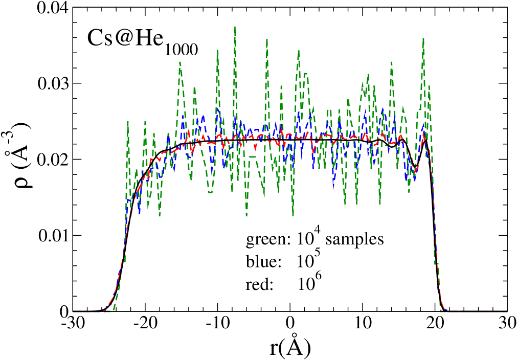
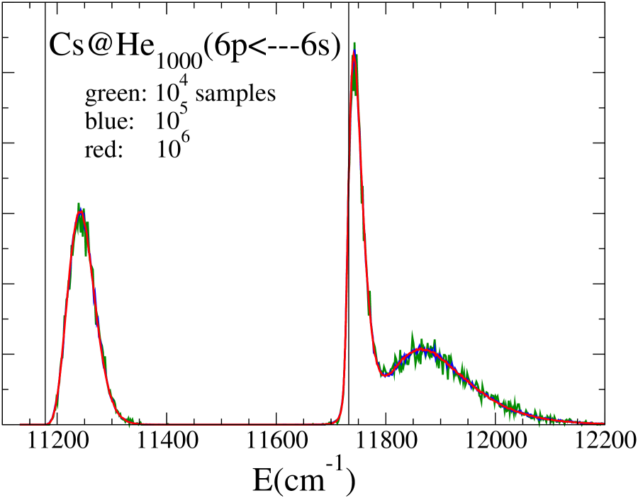
Figure 5: (a) DFT density profile along the $z$ axis [$\rho(z)$] of the Cs@⁴He₁₀₀₀ droplet (solid line) and the simulated profile corresponding to $n_{c}=10^{4}$ (green), $10^{5}$ (blue), and $10^{6}$ (red) simulations. (b) $6p\leftarrow 6s$ absorption spectrum of Cs obtained using the corresponding sampled density distribution. The Patil He-Cs potentialPat91 has been used for the ground state and the Pascale He-Cs potentials for the excited states.Pas83 The spectrum is given in arbitrary units; in the cases of $n_{c}=10^{4}$ and $10^{5}$, it has been multiplied by a factor of 100 and 10 respectively so that they can be compared to that of $n_{c}=10^{6}$.

Optical absorption and fluorescence spectroscopy of doped helium droplets establishes an important link between experiments and theory. Not only does it provide a test to validate the applied theoretical method, but it can also give a microscopic view into the associated dynamics. The latter aspect has, for example, been used to establish the details of impurity solvation in helium droplets (e.g. interior vs. surface solvation).Sti99

Provided that the helium dynamics does not contribute to the spectrum significantly, the transition energies can be approximated with the eigenvalues of $U_{T}$ defined after Eq. (41). Within this model, line broadening originates from fluctuations in the helium densityMat11b and/or the zero-point density distribution of the impurity $|\phi(\mathbf{r}_{I})|^{2}$.Her10 An outline of the former case is given below (‘DF sampling method’).

Within the Born-Oppenheimer approximation, electronic and nuclear degrees of freedom are treated separately. The absorption and fluorescence line shapes can then be calculated by Fourier transforming the helium bath time-correlation function.Tan07 Within the semi-classical approximation,Her08a the absorption line shape function $I(\omega)$ is

$$I(\omega)\propto\sum_{m}\int\mathrm{d}^{3}\mathbf{r}~{}|\phi^{\mathrm{gs}}(\mathbf{r})|^{2}\delta\left[\omega-(V^{\mathrm{ex}}_{m}(\mathbf{r})/\hbar-\omega^{\mathrm{gs}})\right]$$ (59)

where ‘ex’ and ‘gs’ refer to the electronic excited and ground states, respectively. The DF sampling method constructs this expression stochastically by generating a large number of helium-impurity configurations ($n_{c}\approx 10^{6}$). Each configuration consists of $N$ helium atoms positions and, if the impurity is light, its position as well. For helium, these coordinates are randomly generated by importance sampling using the DFT helium one-particle density $\rho(\mathbf{r})/N$ as the probability distribution, where short-range correlations from the hard-sphere term are also considered. The impurity positions are sampled using the zero-point distribution $|\phi^{\mathrm{gs}}(\mathbf{r}_{I})|^{2}$. Such sampling is obviously not required for classical impurities.

Fig. 5 shows the one-particle density generated by importance sampling, compared to the calculated by DFT in the case of a (classical) Cs doped ⁴He₁₀₀₀ droplet, using $n_{c}=10^{4},10^{5},$ and $10^{6}$ configurations. Examples considering the impurity quantum mechanically can be found in Refs. Her10, ; Her11, .

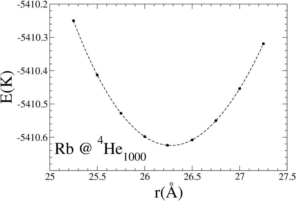
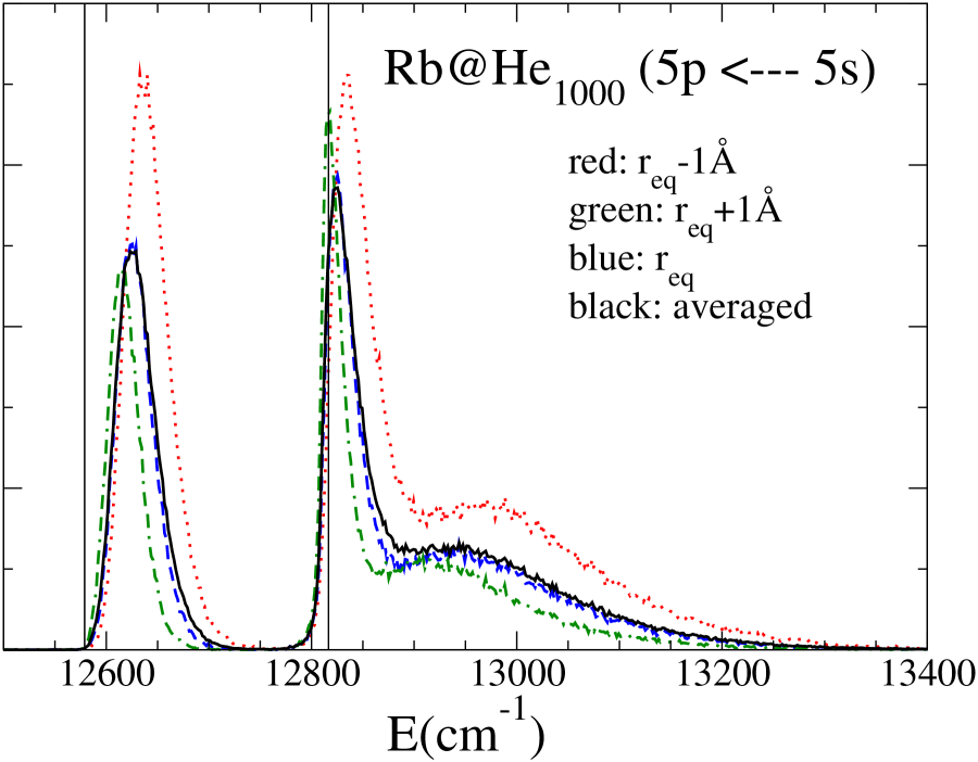
Figure 6: (a) Energy of Rb@⁴He₁₀₀₀ as a function of the distance of the Rb atom from the COM of the droplet; the equilibrium position of Rb is $r_{eq}$=26.24 Å. (b) Absorption dipole spectrum (arbitrary units) for several locations of the Rb atom shown in (a). The number of configurations used to simulate the three spectra is $n_{c}=10^{5}$.

To determine the contribution of each configuration $j$ to the overall absorption spectrum, the corresponding line position is computed from the difference between the excited and ground state energies. The latter is simply taken as the sum of pairwise ground state interactions, $V^{\mathrm{gs}}\{j\}=\sum_{i}V_{X}(|\mathbf{r}^{\{j\}}_{i}-\mathbf{r}^{\{j\}}_{I}|)$, whereas the excited state energy is determined by the eigenvalues of $U_{T}=U+U_{SO}$, where $U_{T}$ was defined after Eq. (41) as the sum of the DIM [Eq. (40)] and the SO hamiltonians. The absorption spectrum is finally constructed as an histogram of the line positions corresponding to each configuration

$$I(\omega)\propto\sum_{m}\,\sum_{\{j\}}^{n_{c}}\delta\left[\omega-(V^{\mathrm{ex}}_{m}\{j\}-V^{\mathrm{gs}}\{j\})/\hbar\right]\;.$$ (60)

As an example, Fig. 5 shows the absorption spectrum for the Cs 6p $\leftarrow$ 6s transition in a ⁴He₁₀₀₀ droplet with $n_{c}=10^{4},10^{5},$ and $10^{6}$. Note that even $n_{c}=10^{5}$ appears to be sufficient to produce a good quality spectrum even though the sampled one-particle density has not fully converged yet. It should be stressed that other sources of broadening such as thermal motion,Her08a coherent helium bath dynamics,Elo04 or droplet size distribution can also contribute to line broadening and are not included in this model.

The influence of thermal motion on the absorption spectrum can be accounted for by considering a thermodynamic ensemble of doped droplets at the experimental temperature of 0.37 K. This is illustrated in the following for Rb doped ⁴He₁₀₀₀ droplets. By constraining the distance between Rb and the droplet COM, the energy landscape seen by Rb can be computed as shown in Fig. 6. The energy corresponding to the experimental temperature of 0.37 K is obtained for distances of $\sim\pm 1$ Å away from equilibrium. Fig. 6 also shows the Rb 5p $\leftarrow$ 5s absorption spectrum corresponding to selected displacements from equilibrium. Indexing them by $i$ and denoting the corresponding spectra by $I_{i}(\omega)$, the thermally averaged spectrum can be constructed as

$$I(\omega)=\frac{1}{{\cal Z}}\sum_{i}I_{i}(\omega)\,e^{-\Delta E_{i}/(k_{B}T)}$$ (61)

where $k_{B}$ is the Boltzmann constant, $\Delta E_{i}$ the energy difference from the equilibrium position, $\Delta E_{i}=E_{i}-E_{eq}$, and ${\cal Z}=\sum_{i}e^{-\Delta E_{i}/(k_{B}T)}$ is the partition function. At 0.37 K the thermally averaged absorption spectrum of Rb is very close to that obtained at the equilibrium position.

Finally, we note that fluorescence spectra can be calculated in a similar way by exchanging the roles of the ground and excited states.Lea16 In this case the DF sampling employs the helium density around the impurity in its excited electronic state instead of the ground state.

V Recent applications of DFT for impurity doped superfluid helium

This section gives an overview of selected results for impurity doped superfluid helium systems obtained with DFT over the past ten years. In addition to covering the wealth of activity on helium droplets doped with alkali and alkaline earth metal atoms, which have been thoroughly studied from both experimental and theoretical points of view, special attention is paid on reviewing the real-time capture of simple atoms by helium droplets (with or without vortex lines) and the dynamics following excitation of impurities attached to helium droplets. Furthermore, other aspects that have also drawn much attention recently, such as soft-landing of doped helium droplets on solid surfaces and the appearance of vortex arrays in helium droplets, are included. Last but not least, impurity dynamics in liquid helium is also considered due to the recent activity in this area. The choice of these topics was motivated by the previous experimental work as well as their successful study by DFT or TDDFT.

V.1 Alkali metal doped helium droplets: solvation and absorption spectra

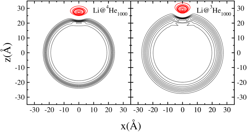
Figure 7: Helium equidensity lines in a symmetry plane of a Li@He₁₀₀₀ droplet. There are nine lines with values ranging from $0.1\rho_{0}$ to $0.9\rho_{0}$ in $0.1\rho_{0}$ steps with $\rho_{0}=0.0218$ Å^-3 for ⁴He, and 0.0163 Å^-3 for ³He. Also shown are equiprobability density lines for Li between $0.001\times\max\{|\phi^{gs}|^{2}\}$ and $0.99\times\max\{|\phi^{gs}|^{2}\}$. Left panel: Li@⁴He₁₀₀₀. Right panel: Li@³He₁₀₀₀.Her11

Since quantum mechanics dominates the behavior of ⁴He droplets, even the solvation of neutral atomic impurities depends on a subtle interplay between the impurity-helium interaction potential and the liquid energetics (e.g. surface tension). A simple procedure to predict whether an impurity solvates in superfluid helium (heliophilic) or resides on the surface of helium droplets (heliophobic) was introduced in Ref. Anc95, . If the impurity is treated classically and interacts with helium through a simple Lennard-Jones potential (‘spherical’ impurity), the solvation behavior can be inferred from the value of a dimensionless parameter $\lambda$

$$\lambda=2^{-1/6}\rho_{0}\,\epsilon\,r_{min}/\gamma$$ (62)

where $\gamma$ is the liquid surface tension, $\rho_{0}$ is the bulk density, and $\epsilon$ and $r_{min}$ are the well depth and equilibrium distance of the Lennard-Jones potential, respectively. DFT calculationsAnc95 suggest that if $\lambda>1.9$ the impurity is heliophilic and solvates inside helium droplets, whereas if $\lambda<1.9$ the impurity is heliophobic and resides on the droplet surface instead. The validity of treating the impurity classically can be assessed by the de Boer parameter $\lambda_{dB}$

$$\lambda_{dB}=\frac{h^{2}}{m\,\epsilon\,r_{min}^{2}}$$ (63)

where $h$ is the Planck constant and $m$ is the impurity mass. For light impurities (e.g. H, Li, Na) $\lambda_{dB}>1$, whereas for heavier impurities that can be treated classically (e.g. Ar, SF₆) the value of $\lambda_{dB}$ is typically less than 0.15.

Based on Eq. (62), all alkali metal atoms have $\lambda$ values much lower than the threshold value $\lambda=$1.9, which indicates that they should reside on the droplet surface.Anc95 This prediction was confirmed by subsequent experimental workSti96 in which the observed impurity line positions were very close to their gas phase values. Surface location is a direct consequence of the very weak binding between alkali metal atoms and helium. The prediction based on Eq. (62) is less conclusive for alkaline earth metals. For example, $\lambda$ is very close to 1.9 for Ca, Sr, and Ba, whereas a value of 2.6 is obtained for Mg. All available experimental evidence indicates that the former species are located on the droplet surface. For Mg the value of $\lambda$ indicates that this species is heliophilic, which is confirmed by both DFT and QMC calculations. This is discussed further in Sec. V.2.

Two major achievements of DFT applied to doped helium droplets are the determination of the resulting solvation structures and the associated optical spectra. In addition to the work reviewed earlier in Ref. Bar06, , joint experimental-theoretical studies on alkali metal atoms from Li to Cs in both ⁴He and ³He droplets have been published since. Impurities were treated either classically (i.e. as an external field)Bue07 or quantum mechanicallyHer10 ; Her11 depending on their masses. Optical absorption spectra in these studies were computed from the Frank-Condon factors,Bue07 the DF sampling method,Her10 or Fourier transformation of the time-correlation function.Her10 ; Her11 In addition, evaluation of time-dependent first-order polarization based on the superfluid helium response has been used for calculating the optical spectrum of intrinsic helium impurities,Elo04 which will be discussed in more detail in Sec. V.8.

The above mentioned studies on alkali metal atoms have demonstrated good agreement with existing experimental results. The calculations were able to reproduce not only the general features of the absorption spectra for ⁴He vs. ³He droplets, but also the fine details observed for Li and Na coupled to either a bosonic or a fermionic helium surface. As an example, Fig. 7 shows the helium density and Li probability density on the symmetry plane of a Li@He₁₀₀₀ droplet (‘dimple’ surface structure). The droplet surface region is contained between the inner and outer equidensity contour lines. Since both the surface tension and the equilibrium density of ³He are smaller than for ⁴He, the surface width of ³He droplets is larger. The resulting dimple solvation structure for other alkali metal-doped ³He₁₀₀₀ and ⁴He₁₀₀₀ droplets can be found in Fig. 3 of Ref. Bue07, .

The dimple solvation structure is deeper on a ³He than on a ⁴He surface. This is a direct consequence of the smaller surface tension of ³He, which also yields a wider surface region. A deeper dimple increases the interaction between the impurity and the droplet. For this reason, the absorption spectra exhibit larger blue shifts in ³He vs. ⁴He droplets. This trend has been observed experimentally and confirmed by DFT calculations, which are also able to reproduce the fine details in the spectra. For example, in addition to the different absorption line shifts observed for Li/Na doped ⁴He vs. ³He droplets, the appearance of weak sidebands in ⁴He is reproduced by DFT.Her10 ; Bue07 ; Her11 This methodology has also been extended to molecular species such as Li₂.Lac13

Both DFT and QMC calculations for doped-helium systems require an accurate representation of the helium-impurity interaction as input. Since the excited electronic states are typically much higher in energy than the ground state, DFT calculation of solvation structures only requires the ground state interaction. For the spectroscopic applications discussed above, the corresponding excited state interaction with helium must also be known. Since a helium atom usually introduces only a small perturbation to the electronic structure of the impurity, the pairwise potential approximation is often very accurate. Pair potentials can be obtained with high accuracy from ab initio electronic structure calculations such as full configuration interaction or coupled-cluster theory.

When the pair potential approximation is not sufficient, a perturbative configuration interaction (PCI) method can sometimes be employed.Cal11b This method was used for excited states of alkali metal atoms where the electronic degrees of freedom couple significantly to the nearby helium atoms. PCI solves the electronic Schrödinger equation numerically in the valence orbital basis set for a free atom and includes an additional potential due to the valence electron-helium density interaction. This method can be applied to highly excited states of alkali metals where the conventional approach would fail. In a series of joint theoretical-experimental studies, it has been applied to model one- and two-photon spectroscopy of highly excited states of Rb, K, and Cs atoms in ⁴He droplets,Pif10 the spectroscopy of Rydberg states of Na atoms in ⁴He droplets, Log11a and the photoionisation and imaging spectroscopy of Rb atoms attached to ⁴He droplets.Fec12

As an example, Fig. 8 shows the PCI potential energy curves for Na@He₂₀₀₀. Based on these potential energy curves, the electronic excitation spectra of surface bound Na can be calculated and compared directly with experiments. This is demonstrated in Fig. 9 for one-photon excitation spectra of surface bound Na, which were obtained by monitoring Na⁺, NaHe⁺, and NaHe${}_{2}^{+}$ ion masses. Log11a The level of agreement obtained is excellent when PCI potentials are employed. In contrast, simulations based on pairwise additive potentials (not shown) considerably overestimate the helium induced spectral shift. This difference can be attributed to helium-induced mixing of the electron configurations.Log11a

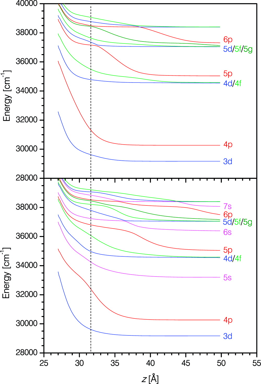
Figure 8: Effective interaction potential curves obtained by the PCI method for a Na atom attached to a ⁴He₂₀₀₀ droplet. Upper panel: $\Pi$ symmetry states. Lower panel: $\Sigma$ symmetry states. The dotted line gives the average distance between the sodium atom in the ground state and the center of the helium droplet.Log11a

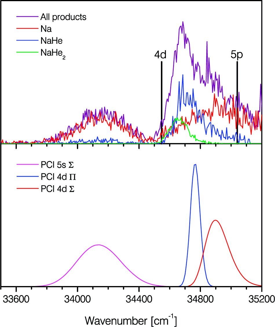
Figure 9: Upper panel: Experimental excitation spectra of sodium attached to helium droplets recorded by monitoring the yield of Na⁺, NaHe⁺, and NaHe${}_{2}^{+}$ ions (arbitrary units). The positions of the free atom transitions are indicated by vertical lines. Lower panel: Theoretical spectra obtained by DFT employing PCI potentials.Log11a

Spectroscopy of alkali metal atoms located on the surface of helium droplets has provided a wealth of detailed information on these systems.Sti06 ; Cal11a ; Mud14 In addition to fluorescence excitation and emission spectra, angular distributions of the ejected atoms have been measured .Log11a ; Her12a ; Fec12 Considering the impurity-droplet system as a pseudo-diatomic molecule, these experiments can clearly distinguish between the $\Sigma$ and $\Pi$ states of the system. Alignment of the electronic angular momentum $\mathbf{j}$ for Na^∗(3p ²P_3/2) obtained by photoejection from ⁴He₂₀₀ droplets was modelled in Ref. Her13, . Together with the angular distribution parameter $\beta$, the coefficient for alignment of $\mathbf{j}$ was obtained from the simulation of the fragment state-resolved photoabsorption spectrum. The alignment coefficient exhibits clear oscillations as a function of the excitation energy. These oscillations were attributed to coherent population of the dissociative $\Sigma$ and $\Pi$ states within the Franck-Condon region. They could be observed experimentally through fluorescence polarization, provided that their dependence on the droplet size is not very strong as this could wash them out by averaging. They could also be visible in the photoelectron yields following ionisation of the atomic fragment. These predictions have not yet been confirmed by experiments.

The helium degrees of freedom are often involved in the relaxation of photoexcited impurities. As discussed before, optical excitation of Na $3$p $\leftarrow 3$s transition populates the pseudo diatomic $\Sigma$ and $\Pi$ states on the droplet surface. It was shown that $\Pi$ state excitation produces both bare Na and NaHe_n exciplexes.Log15 Based on their measured velocity distributions, the bare Na atoms appear to be produced by an impulsive mechanism whereas exciplex production is thermally driven. The $\Sigma$ state is very repulsive and leads to impulsive desorption of bare Na.Log15 Based on the spin-adiabatic approximation, these bare atoms should only be produced in the ²P_3/2 state. However, the experiment measured population in both the ²P_3/2 and the ²P_1/2 states. This has been attributed to a curve crossing taking place between the pseudo-diatomic states at long range.Log15 Similar curve crossings have also been reported for other alkali metal-rare gas systems.Ger16

V.2 Alkaline earth metal doped helium droplets: solvation and absorption spectra

Helium droplets doped with alkaline earth metals have been experimentally studied and modeled by DFT. Due to their larger binding towards helium as compared to heliophobic alkali metal atoms, the resulting solvation structure depends on the species considered and on the isotopic composition of the droplet. DFT calculations predict that alkaline earth atoms from Mg to Ba reside inside ³He droplets; Ca, Sr, and Ba occupy dimple states on the ⁴He droplet surface, and Mg is heliophilic.Her07 The DFT results are consistent with the available spectroscopic data for ⁴He droplets, see Ref. Her07, and references therein. No data is available for Be but it is presumably heliophilic.

Large helium droplets made up of a few thousand atoms may host vortex lines that are created during the gas condensation phase. Since trapping of impurities at vortex lines alters the surrounding liquid density distribution, it has been proposed that absorption spectroscopy of alkali metal atoms, excited state helium atoms, or electrons could be used to detect vorticity.Clo98 ; Mat10b ; Mat15a Unfortunately, the spectral changes are predicted to be very small. For this reason, the Ca atom may be a better candidate because it is just barely localised on the droplet surface.Sti97 ; Her08a In the presence of a vortex line, Ca atoms could be drawn into the vortex core and sink inside the droplet.Anc03 Such a change in the solvation environment should produce a more pronounced effect in the absorption spectrum. Indeed, DFT calculations confirm this idea and the predicted changes in the absorption spectra are shown in Fig. 10.Her08a However, the experimental absorption spectrumSti97 does not exhibit any structure that could be attributed to the presence of vortices to which Ca atoms are attached. It was concluded that the proportion of droplets with vortex lines in the beam is probably too small to produce a noticeable effect in the spectrum. Note that vortex arrays in large helium droplets have been observed experimentallyGom14 ; Jon16 ; Ber17 and modelled by DFT.Anc15 This will be discussed in more detail in Sec. V.13.

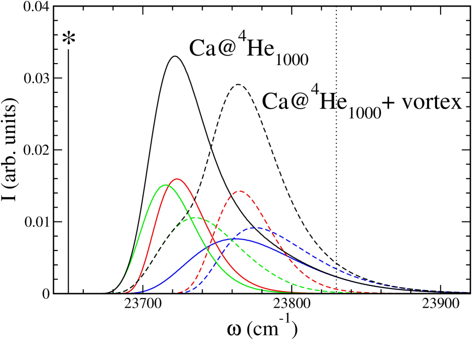
Figure 10: Absorption spectrum of Ca in the ⁴He₁₀₀₀ droplet with (dashed lines) and without (solid lines) a vortex line along the symmetry axis.Her08a The absorption spectrum (black) is split into the $\Sigma$ (blue) and $\Pi$ components (green and red). The starred vertical line represents the gas-phase line position and the dotted vertical line represents the experimental value for bulk liquid ⁴He.Mor05

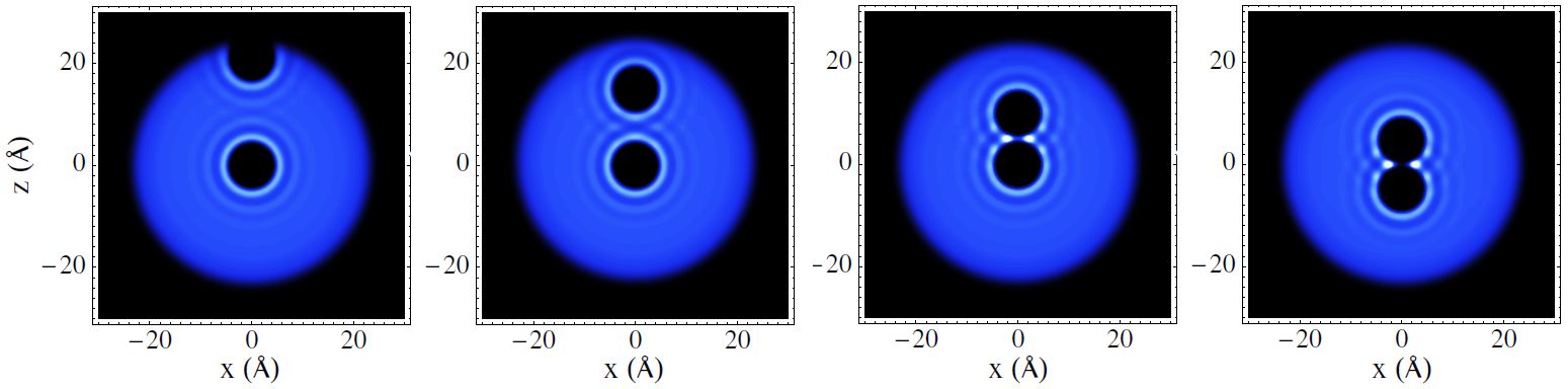
Figure 11: From left to right, (Mg+Mg)@⁴He₁₀₀₀ metastable configurations for Mg–Mg interatomic distances 18.5 Å, 12.9 Å, 9.3 Å, and 9.5 Å. The corresponding total energies are $-$5567.8 K, $-$5573.9 K, $-$5580.3 K and $-$5581.4 K, respectively. The bright regions correspond to high density helium.Her08b

Calculations of Mg atom-doped ⁴He droplets have revealed an interesting solvation behavior as a function of the droplet size, indicating that Mg atoms are highly delocalised in the ⁴He droplets. Indeed, DMC calculations for small droplets up to $N_{4}=50$ predict that Mg is not fully solvated below $N_{4}\sim 30$.Mel05 ; Nav12 Recent PIMC calculations have found that Mg atoms are solvated in ⁴He₁₀₀ droplets.Kro16 thus confirming that the droplets must have at least several tens of helium atoms to fully solvate the Mg atom. DFT calculations for small and large helium dropletsHer07 ; Her08b are in agreement with the QMC findings. These results are also consistent with the analysis of Laser Induced Fluorescence (LIF)Reh00 and Resonant Two-Photon-Ionisation (R2PI) experiments.Prz08 For very large droplets, $N_{4}\sim 10^{4}$, electron-impact ionisation measurements suggest that Mg atoms are located on the surface,Ren07 which is in clear disagreement with the previously mentioned LIF and R2PI experiments and with the calculations. The origin of this discrepancy has not been identified yet.

When ⁴He droplets are doped with more than one impurity, their free motion and strong mutual attraction are expected to lead to efficient clustering inside the droplet. The formation and properties of metal clusters isolated in helium droplets has been reviewed in  Ref. Tig07, . If the long-range part of the impurity-impurity interaction becomes comparable to that of the impurity-helium interaction, a dilute loosely bound ‘bubble foam’ structure (also called ‘quantum gel’) may form Ref. Prz08, . Such a foam consists of separated impurities trapped in their own solvation bubbles within the droplet. A similar scenario was put forward to explain experimental findings related to the successive capture of impurities in helium dropletsLew95 and in the bulk liquid.Gor04

The first DFT calculation to model the formation of bubble foam in bulk superfluid helium was carried out for Ne atoms.Elo08 The Ne-He interaction is strong enough to produce a localised solvent shell structure around Ne. The calculated interaction energy as a function of the distance between two Ne atoms, including the liquid contribution, exhibits local maxima when the solvent shells centered around each atom overlap. This creates a liquid induced energy barrier to recombination, which may localise the atoms far away from their gas phase equilibrium positions, provided the barrier is higher than the thermal energy. Similar calculations have been published for Ag-Ag, Cu-Cu, Au-Au, and F-F interactions in superfluid helium.Hau15 ; Elo11 One of the goals in these studies was to address the timescale for metal-cluster formation in ⁴He droplets by using a mixed DFT-classical molecular dynamics approach.Hau15

Motivated by the experimental work on multiply doped Mg droplets,Prz08 the above mentioned DFT approach was also used to study Mg-Mg recombination in ⁴He₁₀₀₀ droplets.Her08b By carrying out the same calculation for ³He droplets where the solvation shells are less pronounced, it was conclusively shown that the solvent shell structure around the impurity plays a key role in the foam formation. As an example, Fig. 11 shows several configurations for (Mg+Mg)@⁴He₁₀₀₀. Note that a ring of high density helium forms around the diatomic axis (see also Ref. Elo08, ; Prz08, ). The extreme right configuration, where the Mg-Mg distance is 9.5 Å, corresponds to the metastable foam configuration. At shorter Mg-Mg distances the energy increases and prevents the recombination into the Mg₂ dimer.Her08b Based on experimental data, this metastable complex collapses into a tightly bound cluster in ca. 20 ps.Prz08 The response of Mg atoms embedded in ⁴He nanodroplets was later studied by femtosecond dual-pulse spectroscopy, which yielded results consistent with the hypothesis of isolated atoms arranged in a foam-like structure.God13

The effect of the above bubble foam configurations on LIF and R2PI spectra in ⁴He droplets was found to be in good agreement with the experimental data, as shown in Fig. 12.Her08b The experiments show that doping helium nanodroplets with more than one Mg atom leads to a shift of the atomic absorption line from 279 nm to 282 nm due to the additional perturbation produced by the neighboring Mg solvation bubbles.Her08b It is worth mentioning that recent QMC calculations on the Mg pair in ⁴He droplets did not yield any barrier for dimer formation;Kro16 no alternative interpretation for the R2PI experiments was presented.

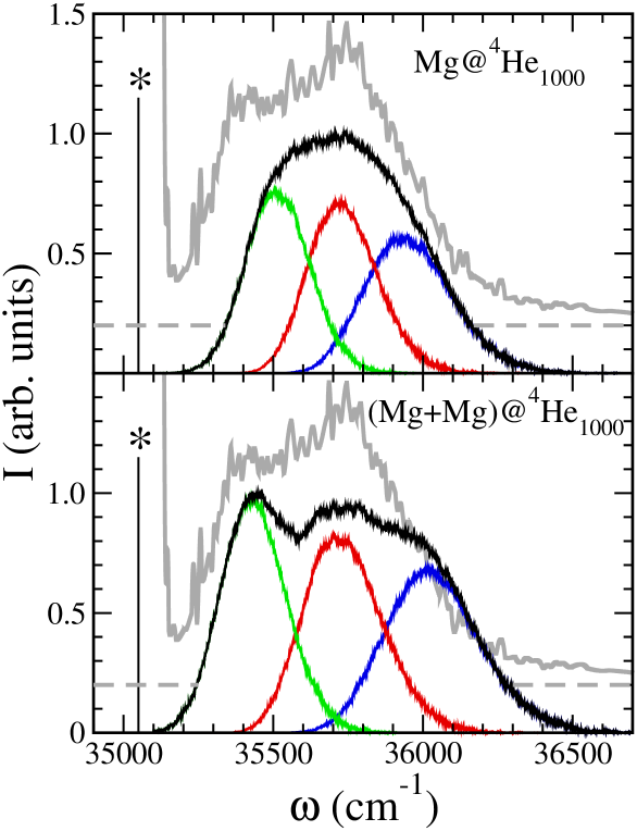
Figure 12: Top panel: 3s3p ¹P₁ $\leftarrow$ 3s^2 1S₀ absorption spectrum of a single Mg atom in a ⁴He₁₀₀₀ droplet. The starred vertical lines indicate the position of the corresponding gas-phase transition. The experimental curve is shown in grey.Reh00 Bottom panel: Same as top panel but the Mg atom resides in a distorted environment created by the presence of another nearby Mg atom.Her08b ; Her09a

The foam structures correspond to loosely bound clusters. Clusters may grow inside helium droplets with different structures, depending on the size of both the droplet and the cluster itself. The formation of Ag clusters up to a few thousand atoms in He droplets was studied via optical laser spectroscopy.Log11c It was found that small Ag clusters ($N_{\rm Ag}\sim 100$) exhibited a plasmon resonance at about 3.7 eV, similar to that previously obtained for dense spherical clusters. However, larger Ag clusters ($N_{\rm Ag}>1000$) formed in ⁴He${}_{N_{4}}$ droplets, $N_{4}\sim 10^{7}$, exhibited an unusually broad spectrum extending into the infrared spectral range. The dramatic change in the spectrum has been associated with a transition from single-cluster to multi-centre growth regime when the droplet size increases. The structure of the cluster aggregates formed inside He droplets remains unknown; it is conceivable that they are loosely packed and may even exhibit a fractal-like structure.

V.3 Droplets doped with more than one species

Helium droplets doped with two different impurity species with opposite solvation behavior have been investigated by DFT. Such studies have been inspired by experimental work showing that an otherwise heliophobic Ba atom could be solvated in helium droplets which already contain a heliophilic xenon cluster in their center.Lug00

In a joint experimental and DFT work,Dou10 droplets doped with HCN-M (M$=$Na, Ca, and Sr) have been studied. The calculations for these systems show a strong surface-bound state for Na, a purely solvated state for Ca, and both surface and solvated states separated by a barrier for Sr. The results for Ca and Sr were consistent with the appearance of the infrared spectrum for these complexes.

In another joint experimental and theoretical project,Mas12 ; Her12b the influence of heliophilic argon doping on the solvation of heliophobic calcium atoms in helium droplets has been studied. The experiment considered the photodissociation of Ca₂ to Ca(4s4p ¹P) + Ca(4s^{2 1}S) in the presence of a varying number of Ar atoms in the droplet. The absorption and emission spectra of Ca-Ar_M ($M=0-7$) complexes were calculated by using the DF sampling method described in Sec. IV.3 with the Ca and Ar atoms treated classically. It was found that even a single Ar atom is enough to trigger Ca atom sinking into the He droplet, where they form a Ca₂ dimer. Furthermore, by studying the emission spectrum as a function of the droplet size (Fig. 13), it was concluded that the emitting species was Ca^∗Ar_M attached to the droplet that has shrunk down to a size less than 200 helium atoms by either evaporation or detachment of helium atoms from the complex.

In another DFT study,Pom12 a heliophilic Xe atom was placed in the bulk of a ⁴He₅₀₀ droplet with a heliophobic Rb atom located on the surface. The Rb-Xe van der Waals attraction was not sufficiently high to overcome the 23.4 K barrier induced by the presence of helium between the dopants and therefore Rb remained on the surface. Clearly, this is a droplet-size dependent effect. Furthermore, it was concluded that the order in which the dopants are introduced to the droplet plays an important role in the formation of such dimers, as they can only form on the droplet surface. In a recent study,Ren16 evidence has emerged that sodium and cesium clusters, and even single Na atoms (but not Cs), can enter ⁴He droplets (average size $N_{4}\sim 5\times 10^{5}$) in the presence of a fully solvated C₆₀ fullerene.

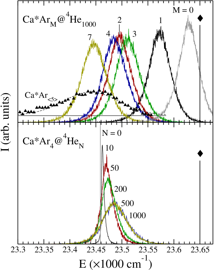
Figure 13: Overview of Ca^∗-Ar_MHe_N ¹P$\rightarrow^{1}$S fluorescence emission spectra obtained by DFT. The upper panel shows the emission spectra for varying number of Ar atoms $M$=1, 2, 3, 4, and 7 in a ⁴He₁₀₀₀ droplet. The bottom panel shows the dependence of the Ca^∗-Ar₄ spectrum on the number of helium atoms in the droplet ($N$). The grey, vertical line labelled $N=0$ indicates the position of the isolated Ca^∗Ar₄ vertical emission. The line labelled with a diamond is the atomic Ca^∗ emission line. The triangles in the upper plot are experimental data for $\langle M\rangle$=5 (hence a Poisson distribution of sizes with a weight of e.g. 0.03 for $M=1$, 0.08 for $M=2$, 0.14 for $M=3$, 0.18 for $M=4$ and $5$, 0.15 for $M=6$, 0.10 for $M=7$). The lower plot shows that, if the emitting species is inside a smaller droplet, the calculated spectra would shift by about 20 cm^-1 to the red, giving a better agreement with experiment. Mas12 ; Her12b

V.4 Cluster-doped helium droplets

Despite their practical and conceptual importance,Tig07 theoretical studies simulating atomic clusters embedded in helium droplets are scarce. A major difficulty in these studies is to obtain reliable cluster-droplet interaction potentials. Besides the work on Ca-Ar_M clusters mentioned before,Mas12 ; Her12b the interaction of two Ne clusters in liquid ⁴He has been studied in Ref. Elo08, . Furthermore, Path-Integral MC (PIMC) calculations of Mg and Na clusters in both helium droplets and the bulk liquid have been carried out.Hol15 These calculations show that Mg clusters are heliophilic whereas small Na_M clusters with $M=7,9$ remain on the surface. Recall that a single Mg atom is also heliophilic when $N_{4}\lesssim 30$.

Alkali atom clusters are especially interesting because the individual atoms reside on the droplet surface whereas larger clusters may become heliophilic and sink inside the droplet. The critical cluster size $N_{c}$ for switching from heliophobic to heliophilic behavior has been determined from the energy balance between the metal-helium van der Waals attraction, the short-range repulsion, and the liquid surface tension.Sta10 The following values have been predicted for $N_{c}$: Li,Na/⁴He $\sim$20; Rb/⁴He $\sim$100; Li,Na/³He $\sim$5; and Rb/³He $\sim$20 The values of $N_{c}$ in ³He are smaller than in ⁴He because of the lower value of the surface tension and saturation density. The prediction for Na in ⁴He droplets was later confirmed by the experiments;Lan11 a recent study on the submersion of Na clusters in ⁴He and para-H₂ clusters employing path-integral molecular dynamics has also found the submersion of Na_N clusters in ⁴He droplets around $N\sim 20$.Cal17

Superfluidity of the helium surrounding Mg₁₁ clusters in ⁴He droplets consisting of up to a few hundred helium atoms has been studied by QMC.Hol14 Furthermore, the commensurate-incommensurate transition of the ⁴He atoms adsorbed on the surface of C₂₀ and C₆₀ was characterised by PIMC.Kwo10 ; Shi12

In a more approximate way, the dissociation dynamics of neon clusters upon ionisation has been studied in a ⁴He₁₀₀ droplet using molecular dynamics corrected for delocalisation of the helium atoms and DIM based interaction potentials.Bon07 ; Bon08 The results showed two interesting processes, one in which the ionic core of the cluster, usually Ne${}_{2}^{+}$, is expelled from the rest of the droplet, and another showing a very efficient cooling effect by helium atom ejection rather than evaporation, with a wide kinetic energy distribution.

Sequential doping of helium droplets allows for the synthesis of core-shell clusters (‘nanomatryoshkas’). Bimetallic clusters have been formed via sequential pickup of gold and silver atoms by helium droplets.Moz07 The resulting structure persists upon ‘soft-landing’ of the clusters on a solid surface. Another nanomatryoshka, made of an Ag core coated by a shell of ethane molecules, has been studied.Log13 These systems are currently beyond the reach of a DFT-based description.

The DFT approach has also been used to simulate the solvation of single-walled carbon nanotubes consisting of up to 360 carbon atoms in a ⁴He₂₀₀₀ droplet using an ab initio He-nanotube interaction potential,Hau16 see also Ref. Hau17, . Depending on the nanotube diameter, the outer and inner walls are covered by one or more dense layers of helium. This structure, which was also found earlier on He-wetted graphite,Cle93 forms as a consequence of the strong surface-He interaction and geometric effects.Hern11

V.5 Doped mixed ³He-⁴He and ³He droplets

Experiments employing mixed helium droplets have been integral to the discovery of ⁴He droplet superfluidity by rotational spectroscopy.Gre98 At low temperatures the two isotopes separate such that the inner part of the droplet consists of ⁴He whereas ³He resides on the outside.Bar06 Depending on the strength of the impurity-He interaction, the impurity may reside on the droplet surface, at the ³He-⁴He interface, or fully solvated inside the ⁴He core.Mat11b ; Bue09

The structure and energetics of small mixed He droplets doped with Mg and Ca impurities has been studied by the quantum Diffusion Monte Carlo (DMC) method with the aim of determining their solvation behavior in pure ⁴He and ³He droplets.Nav12 ; Gua09 Since Ca is heliophilic in ³He droplets but heliophobic in ⁴He, it was expected to reach the ⁴He core surface while remaining inside the ³He shell. This is indeed confirmed by DFT calculations as illustrated in Fig. 14 for Ca@⁴He₅₀₀+³He${}_{N_{3}}$ droplets.

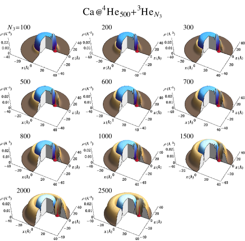
Figure 14: A three-dimensional view of Ca@⁴He₅₀₀+³He${}_{N_{3}}$ helium droplets with $N_{3}$ varying from 100 to 2500. The ⁴He core and ³He shell are pictured in blue and in brown, respectively. The probability density of the Ca atom is also displayed along the density cut (red spot; specified in arbitrary units).

The interfacial location of Ca has also been verified by independent QMC calculations and absorption spectroscopy experiments.Gua09 ; Bue09 Figure 15 shows the calculated spectral shift and full width at half maximum (FWHM) as a function of the number of ³He atoms $N_{3}$ for $N_{4}$ = 1000. Direct comparison with experimental data is difficult because the ³He-⁴He composition of the gas used may not directly carry over to the droplets.Bue09

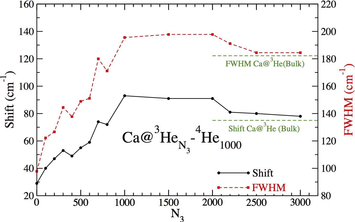
Figure 15: Calculated shift and full width at half maximum (FWHM) of the Ca absorption spectrum around the 4s4p$\leftarrow$4s² transition as a function of the number of ³He atoms $N_{3}$ for $N_{4}$ = 1000.Bue09

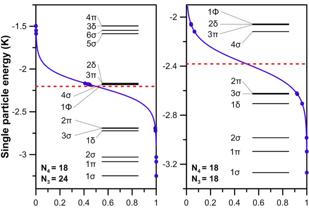
Figure 16: Single-particle energies $\epsilon_{i}$ (vertical scale, K) of the ³He component of an OCS@³He${}_{N_{3}}$+⁴He₁₈ droplet for two selected values of $N_{3}$.Lea13 The dashed line represents the ³He chemical potential $\mu_{3}$. The occupation numbers are represented by dots (horizontal scale) and the line connecting them represents the function $n_{i}=1/\{1+exp[(\epsilon_{i}-\mu_{3})/k_{B}T]\}$.

Interatomic Coulombic decay (ICD)Ced97 has been proposed as a tool for studying the interface of isotopically mixed helium droplets doped with Ca atoms,Kry13 since ICD is highly sensitive to the solvation environment. In a previous ICD study, isotopically pure ³He and ⁴He droplets doped with Ne and Ca were studied.Kry07 The aim was to provide observables that would be sensitive to helium density around the impurity atom and compare them with DFT results. The first experimental study of ICD in ⁴He nanodroplets, induced by photoexcitation of the $n=2$ excited state of ⁴He⁺, has been carried out recently.Shc17 It was found that the ⁴He⁺ kinetic energy distribution was strongly affected by the droplet environment, depending on whether ICD occurred inside the droplet or within the droplet surface region.

In DFT calculations of large mixed helium droplets, the kinetic energy of the ³He component is treated using the Thomas-Fermi-Weizsäcker approximation, where the kinetic energy density is written as a sum of two terms, one proportional to $\rho_{3}^{5/3}(\mathbf{r})$ and the other proportional to $(\nabla\rho_{3})^{2}/\rho_{3}$.Gui93 However, this is only justified for large ³He droplets. For small droplets, the Kohn-Sham (KS) orbitals must be employed, which introduces an additional complication as the systems of interest are not spherical. DFT-KS studies have been published on small mixed helium droplets doped with Ca.Mat09b The single ³He atom excitation spectrum in ⁴He${}_{N_{4}}$ droplets with $N_{4}$= 8, 20, 40, and 50 has been obtained and compared with DMC results,Mat09a and the effect on the ³He excitation spectrum of doping the ⁴He₅₀ droplet with Ca was discussed.

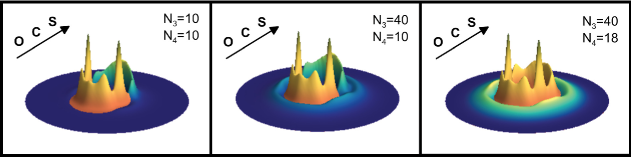
Figure 17: Three-dimensional visualization of the atomic densities around OCS for mixed ³He-⁴He droplets.Lea13 The $N_{3}$ and $N_{4}$ values are indicated. Blue/green gradient represents the density of ³He and orange/yellow gradient the density of ⁴He. The OCS molecule sits at the center and its orientation is indicated schematically.

Despite the conceptual relevance of addressing an OCS molecule embedded inside mixed helium droplets, DFT-KS calculations for the structure of small OCS@³He${}_{N_{3}}$+⁴He${}_{N_{4}}$ systems, where the OCS molecule was treated as an external field, have only appeared recently.Lea13 One interesting aspect of this work is that ⁴He has been described at $T=0$ whereas a finite temperature DFT-KS approach was used for ³He. This can be justified by considering that the elementary excitations of ⁴He droplets are collective and their energies are of the order of several Kelvin, whereas the elementary particle-hole excitations of ³He have energies comparable to the temperature of the experiment ($\sim$ 0.1 K for OCS doped ³He droplets).Sar12 Since mixed droplets cool down by evaporation from the ³He free surface, a similar temperature to the previously mentioned particle-hole excitation energy is expected for mixed droplets. Such a small temperature has a negligible effect on the bosonic component of the droplet, but it may influence the fermionic component provided that the level spacing of the single-particle (s.p.) energy levels is of the order of $k_{B}T$. In this case, a large density of states with fractional occupation $n_{i}$ is expected around the Fermi level.

Given an ensemble $\{n_{i}\}$ that fulfills $N_{3}=\sum_{i}n_{i}$, the standard deviation of $N_{3}$ is given by

$$\Delta N_{3}=\sqrt{\sum_{i}n_{i}\,(1-n_{i})}$$

This quantity exhibits pronounced local minima at ³He shell closures (‘magic numbers’) and local maxima at $N_{3}$ values that correspond to half-filled shells. Notice that $\Delta N_{3}=0$ when all the occupation numbers are either 0 or 1.

Figure 16 shows the s.p. structure of the ³He component of an OCS@³He${}_{N_{3}}$+⁴He₁₈ droplet with $N_{3}=18$ and 24. Notice that $N_{3}=18$ corresponds to a closed-shell configuration whereas $N_{3}=24$ is a half-filled shell. Accordingly, the level scheme in Fig. 16 displays a fairly large energy gap around the Fermi level for $N_{3}=18$ and shows both large and small occupations. In contrast, the spectrum for $N_{3}=24$ is dense around the Fermi level with several s.p. states partially occupied. Since the energy gap is small in open shell droplets, their proper description must include thermal effects. Other examples are discussed in Ref. Lea13, . Helium density distributions around the OCS molecule for three selected configurations are shown in Fig. 17.

Helium-3 droplets doped with OCS have been investigated within DFT-KS.Mat13a This work was motivated by the analysis of experimental infrared spectroscopy data for the OCS molecule embedded in ³He${}_{N_{3}}$ droplets with $N_{3}\sim 1.2\times 10^{4}$.Gre98 ; Sar12 Before this experiment, only the glyoxal molecule had been studied in ³He droplets through the excitation of electronic and vibronic transitions. It was observed that the zero phonon lines (ZPL) were accompanied by additional broad bands on their red side due to particle-hole excitations of the droplet.Poe09 Furthermore, a small sharp peak superimposed on the additional band was assigned to vibrations of the snowball structure that surrounds the molecule. These particle-hole excitations accompanying the ZPLs were further analysed in Ref. Ben12, .

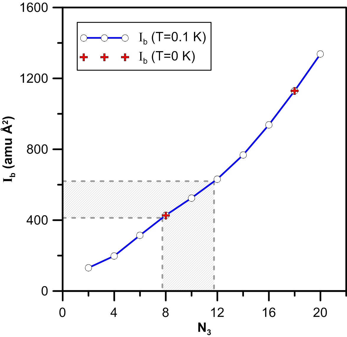
Figure 18: Rigid moment of inertia of OCS@³He${}_{N_{3}}$ (in amu Ų) perpendicular to the symmetry axis as a function of $N_{3}$.Lea13 The shaded area indicates the experimental values;Sar12 the $T=0$ values are from Ref. Mat13a, .

While the Q-branch is missing in the infrared spectrum of OCS in both ³He and ⁴He droplets, the effective moment of inertia (MOI) in ³He is approximately twice as large as compared to ⁴He. Note that this value is 5.5 times larger than observed in the gas phase. The increase in MOI was attributed to the presence of an evenly distributed shell of 11 ³He atoms around the molecule.

The structure and energetics of small OCS@³He${}_{N_{3}}$ droplets was studied in Ref. Mat13a, by using the functional described in Ref. Bar97, . Similarly to the previously discussed calculations, the OCS molecule was incorporated into the model as an external potential. Since the calculation was carried out at $T=0$, it was restricted to small $N_{3}$ values that correspond to closed-shell OCS@³He${}_{N_{3}}$ droplets, $N_{3}=8,18,$ and 40. The ³He atoms are expected to fill the waist around OCS between the O and C atoms. The calculated number of atoms present in this ring was about 4 for ³He droplets and 5 for ⁴He droplets.

The distribution of He atoms around the OCS molecule affects its rotational properties. The MOI for OCS attached to ³He${}_{N_{3}}$ droplets with $N_{3}=8$, 18, and 40 was calculated by the rigid body expression and the results were compared with ⁴He data. The calculated MOI of OCS@³He${}_{N_{3}}$ is shown in Fig. 18.Lea13 Comparison with $T=0$ results shows that the small non-zero temperature in the calculations does not influence the morphology of the fermionic droplet, but allows to carry out the calculations for any $N_{3}$ value and not only for the magic numbers.

V.6 Electrons in liquid helium

Figure 19: Top panel: Electron bubble density profile (right scale) and electron probability density for the 1s, 1p, 2p and 3p states (left scale) at $P=T=0$ in superfluid ⁴He. Bottom panel: The corresponding confining potential well and single-electron energies.Bar13

DFT has been succesfully used to study excess electrons and homogeneous cavitation in liquid ⁴He and ³He. Analysis of phenomena such as the crossover from thermal to quantum cavitation in liquid ⁴He, heterogeneous cavitation by excess electrons, and the effect of vorticity on these processes have been presented in the literature.Bar02 ; Bal02 ; Mar08

Any impurity embedded in liquid helium, including an electron, must loose its excess kinetic energy by ionisation of helium atoms and/or excitation of the liquid excitation modes. After the electron has lost most of its kinetic energy and moves at a velocity below the speed of sound in the liquid, it produces a cavity (‘bubble’) and becomes localised in it. In liquid ⁴He, this cavity – which is void of He atoms at $T=0$ – has a radius of $\sim 19$ Å and is the result of the competition between the zero-point energy of the confined electron, the surface energy of the bubble, and the work done against the liquid pressure for creating the cavity.

Figure 19 shows the helium density profile around the electron at $P=T=0$ along with the electron probability densities for 1s, 1p, 2p, and 3p states, and the confining potential. The 3p state is barely bound under SVP as its energy is just below the free electron limit, and it becomes delocalised above 1.7 bar.Bar13 The energy differences between the np and 1s electron levels correspond to the peak maxima in the electron absorption spectrum.

The properties of electron bubbles (e-bubble) in liquid helium have been reviewed in Ref. Mar08, ; Tab97, ; Cou09, ; Mar00, ; Mar15, with the more recent articles concentrating specifically on the identification of the experimentally observed unusual negative species (‘exotic ions’). Furthermore, multi-electron bubbles in liquid helium have also been studied and their properties reviewed in Ref. Tem07, . It was shown that highly charged multi-electron bubbles are unstable against fission at positive pressures.Guo08 The production of long-lived multi-electron bubbles at negative pressures has been reported recently.Fan17 A major difficulty in these studies is that the radius of the bubble must be on the micron-scale so that the electron-electron Coulomb repulsion can be reduced. So far, only two-electron bubbles have been modelled with DFT,Leh07 and the conclusion was that they are unstable and break into two separate electron bubbles. No real-time simulation of this process has been carried out yet.

While there is no direct way to measure the properties of electron bubbles, absorption measurements can provide relative energetics for the electron level structure. The DFT calculations performed in Refs. Elo02, ; Gra06, are in excellent agreement with the experimental absorption data of Grimes and Adams.Gri92 Furthermore, DFT calculations are able to reproduce the experimentally observed negative pressure required to explode electron bubbles in the liquid.Cla98 ; Pi05 These comparisons confirm that the combined electron and DFT model can capture the essential physics of the e-bubble state.

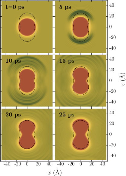
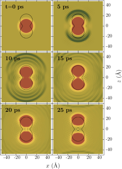
Figure 20: (a) Adiabatic evolution of the 1p e-bubble at $P=0$. The panels display the helium configurations at the indicated times. The dashed line represents the dividing surface, which corresponds to half of the helium equilibrium density for the quasi-equilibrium configuration at $P=0$. (b) Same as (a) but for $P=5$ bar.Mat10c

Figure 21: (a) Contour plot showing the stationary state of the e-bubble at $P=0$ corresponding to $v=50.5$ m/s, which is just below the critical value of $v_{c}=50.7$ m/s. The equidensity lines for the ⁴He density (solid lines) are plotted for values between $0.1\rho_{0}$ and $0.9\rho_{0}$ in steps of $0.1\rho_{0}$ with $\rho_{0}=0.0218$ Å^-3. The equidensity lines for the electron probability density (dashed lines) are plotted using nine lines between zero and its maximum value. (b) Surface isodensity plot showing a quantised vortex ring emitted at $P=0$ just above $v_{c}$.Anc10

The structure of e-bubbles hosting an excited electron has been a subject of interest since the experimental work in Refs. Kon03, ; Mar08, was interpreted to involve such states. Furthermore, these bubble structures determine the emission spectrum of the electron bubble. The relevant DFT work on excited e-bubbles was carried out in Refs. Leh07, ; Mat10c, ; Jin10c, . The most interesting excited states are the 1p and 2p states, which can be accessed by experiments. The evolution of the bubble around these states has been computed by DFT.Mat10c In this calculation, the liquid degrees of freedom evolve in real time while a time-independent Schrödinger equation is solved for the $n$p electron at each time step. This adiabatic approximation can be justified by the large helium-electron mass ratio, $m_{4}/m_{e}\sim 7300$. Note that this approximation would fail if level crossings are encountered during the time evolution.

The adiabatic evolution of a 1p e-bubble at $P=0$ and 5 bar is shown in Fig. 20 along with the quasi-static configurations obtained by fully relaxing the liquid. At $P=0$ the adiabatic evolution leads to a quasi-equilibrium configuration whereas at $P=5$ bar the e-bubble splits at the waist. The threshold pressure for the bubble splitting process is $\sim$ 1 bar. This in agreement with the experiments, which indicate that the relaxed 1p bubble is only stable when pressure is smaller than ca. 1 bar.Mar04

The evolution of a 2p state e-bubble at $P=0$ has been studied within the adiabatic approximation.Mat10c The calculations revealed that after 7 ps, the $m=0$ levels of the 2p and 1f states become very close and the adiabatic approximation fails. This indicates that quasi-static electron bubble configurations above 1p cannot be reached. A detailed discussion on the validity of the adiabatic approximation for the electron bubble can be found in Ref. Mat10c, and references therein. Other excited e-bubbles have also been studied by the quasi-static approximation.Mar08 ; Leh07

Real-time propagation of e-bubbles using finite-range functionals such as OT-DFT is computationally unfeasible due their complexity. The use of a zero-range functional as e.g. that of Refs. Str87a, ; Str87b, (ST functional) simplifies the calculation of the mean field potential and reduces the computational demand of the calculation.Mat11a ; Jin10b ; Jin10a ; Jin10c A major shortcoming of zero-range functionals is that they cannot reproduce the maxon-roton portion of the liquid dispersion relation, but only the phonon part up to $q\sim 0.6$ Å^-1.Mat11a Despite this limitation, the evolution of 1p electron bubbles at various pressures with both the zero and finite-range functionals appear fairly similar. This suggests that zero-range functionals can also be applied to study 2p electron bubbles.

Real-time dynamics calculations employing the ST functional have confirmed the two key findings obtained using the adiabatic OT-DFT approximation: 1) the splitting of the 1p e-bubble above $P\gtrsim$1 bar and 2) the failure of the adiabatic approximation for states higher than 1p. The latter finding confirms that quasi-static configurations corresponding to 2p, 2d, $\dots$ do not exist.

Motion of electrons in liquid ⁴He has been studied by Maris et al. using zero-range functionals.Jin10a ; Jin10b They showed that a 1s electron bubble moving at a sufficiently high velocity begins to expand, deforms from the spherical symmetry, and nucleates vortex rings. Energy dissipation did not only arise from the creation of vorticity but also from the excitation of bubble surface modes. These results were confirmed by imaginary-time OT-DFT calculations in the co-moving frame, see Eq. (67).Anc05b ; Anc10 Based on these calculations, the critical velocity for vortex ring nucleation at $P=0$ is $v_{c}=50.7$ m/s. This value is in agreement with the critical electron drift velocity measured at low pressures.Nan85

The complete mechanism of ring vortex nucleation is not yet fully understood. Based on DFT calculations, the e-bubble becomes compressed along the axis of propagation and elongated in the perpendicular direction upon increasing its velocity. Once the bubble exceeds the critical velocity $v_{c}$, a quantised vortex ring emerges from the equator of the bubble where the local liquid velocity is higher. Fig. 21 shows electron bubbles moving at velocities of 50.5 m/s ($<v_{c}$) and slightly above $v_{c}$ (vortex ring emission). Note the significant distortion of the electron bubble geometry that appears below $v_{c}$ (cf. Fig. 19). The interaction of electrons with vortex lines is discussed in Sec. V.12.1.

V.7 Cations in liquid helium and droplets

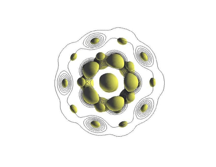
Figure 22: (a) Helium density distribution around a Be⁺ ion in a ⁴He₇₀ droplet shown by constant density surfaces $\rho=0.04$ Å^-3.Anc07 The lines show equidensity contours along a plane passing through the center of the droplet. (b) Average radial helium density of the Be⁺@⁴He₇₀ droplet. Solid line: DFT result; squares: PIMC result.Pao07

Development of new techniques for doping helium droplets with charged impurities allow the controlled study of positive ions in superfluid helium.Sti03 While neutral species could be excited in helium droplets by a resonant laser and detected essentially against a zero background, similar experiments have had limited success for ions. It is only recently that experimentalists have found a way to study the dynamics of photoexcited ions in helium droplets. This technique relies on the ejection of photoexcited ions from the droplets, which increases the yield of unsolvated ions at resonant wavelengths.Bra04

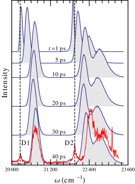
Figure 23: TDDFT time-resolved absorption spectrum of Ba⁺ in a ⁴He₁₀₀₀ droplet.Mat14 The experimental spectrum corresponding to helium droplets with an average size of 2700 atoms is shown in red.Zha12 The vertical lines indicate the D1 and D2 transitions of free Ba⁺.

Figure 24: Snapshots of the temporal evolution of Ba⁺@⁴He₁₀₀₀ after photoionisation of the neutral Ba atom located on the droplet surface.Mat14 From top to bottom and left to right, the panels correspond to helium densities at times $t=$ 0, 8, 14, 47, 60 and 220 ps.

Strongly attractive ions tend to form a solid-like helium layer around them (snowball). Alkali metal ions are believed to belong to this category.Pao07 ; Gal11 In contrast, singly charged alkaline earth cations are expected to produce a cavity due to the outer electron-helium repulsion; thus, they are surrounded by a compressed but less inhomogeneous liquid.Ros04 ; Pao07 ; Lea14b

Alkali metal, alkaline earth metal, and rare gas cations have been recently studied by both experiments and theory.Lan12 ; Bar14 A DMC investigation of Pb⁺ in small He droplets, motivated by the experimental findings of Refs. Tig07, ; Dop07, , is reported in Ref. Sla10, . A similar study was carried out on Na⁺.Iss14 These studies have highlighted the importance of the many-body interactions that arise from charge-induced dipole interaction between the ion and the surrounding helium atoms. Note that this interaction cannot be accounted for by including just the $-\alpha e^{2}/(2r^{4})$ polarization term in the cation-helium pair interaction.

DFT calculations have been used to study the solvation structure of Ba⁺ cation in liquid helium and the stability of the so-called ‘scolium’. Scolium, which was named after Giacinto Scoles,Sti06 consists of an electron orbiting around a small helium droplet that hosts a positively charged ion. The electron cannot penetrate inside the droplet because of the large solvation energy barrier (ca. 1 eV). It was suggestedAnc07 that for small droplets, the pressure exerted by the orbiting electron further increases the local helium density around the ion due to electrostriction, which consequently turns the whole droplet into a solid. It was also shown that the lowest scolium state is unstable, the cation being pulled off from the droplet center towards the surface where it undergoes fast charge neutralization. The neutralization time was estimated to be on the order of a few picoseconds for a 50 Å radius droplet. As an example of cation solvation in a helium droplet, Fig. 22 shows the helium density for a Be⁺ doped ⁴He₇₀ droplet where the ion is located at the center.Anc07 Comparison with the QMC data provided in that figure demonstrates a good agreement between the two methods. Notice that such a good agreement is only possible when the ‘solid’ OT-DFT described in Sec. II.3.1 is used. The conventional OT-DFT produces unphysically large pile-up of helium density around the cation. A similar level of agreement has been found for other cations.Fie12 ; Lea14b The experimental realization of scolium was later achieved by using Na⁺ rather than Be⁺.Log11b

QMC and DFT calculations on Rb⁺ and Cs⁺ cations in helium droplets show that they are fully solvated and develop snowball structures.Ros04 ; Lea14b Based on DFT results, the first solvation shell around Rb⁺ and Cs⁺ hosts 19.2 and 21.4 atoms, respectively. These values are somewhat larger than those found experimentallyMue09 ; The11 as well as by QMC calculations.Gal11 On the contrary, the solvation structure around a Ba⁺ ion was found to be smooth without pronounced structure. This is in agreement with QMC calculations.Pao07 The difference in the solvation structures is a direct consequence of the much weaker interaction between Ba⁺ and helium compared to that of Rb⁺ or Cs⁺ with helium.

In general, cations are solvated in helium droplets because they exhibit very attractive interaction with helium. Based on this observation, experimentalists have studied the sinking of positive ions in ⁴He droplets resulting from the ionisation of heliophobic alkali and alkaline earth metal atoms.The10 ; Log11b ; Zha12 This activity has motivated the corresponding TDDFT simulations of the ion sinking process.Mat14 ; Lea14b ; Lea16

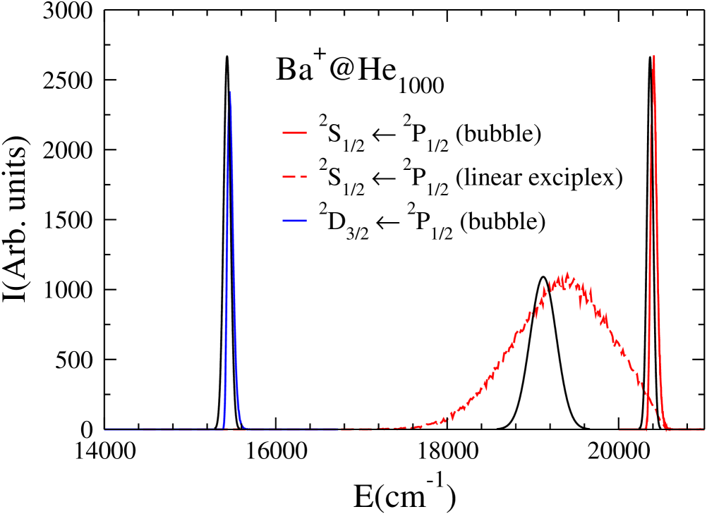
Figure 25: Emission spectrum obtained from de-excitation of the relaxed ²P_1/2 state of a Ba⁺ cation in a ⁴He₁₀₀₀ droplet.Lea16 The gaussian lines shown in black are the experimental results.Rey86

Figure 23 shows the DFT time-resolved absorption spectrum of a Ba⁺@⁴He₁₀₀₀ 6p$\leftarrow$ 6s transition after photoionisation of the surface-bound atom. The experimental dataZha12 show a clear signature of the cation sinking process as the observed spectrum coincides with the corresponding absorption spectrum in the bulk liquid.Rey86 DFT simulations of the ion sinking into the droplet have revealed the nucleation of vortex rings as illustrated in Fig. 24. The snowball structure appears dynamically as bright spots around the cation during the initial solvation process, and wears out when the ion velocity decreases due to kinetic energy dissipation. The latter observation is in accordance with static DFT calculations.Lea14b

In addition to the dynamic formation of the Ba⁺ snowball and the time-resolved absorption spectra of this cation, the most interesting outcome of the calculations is the formation of a vortex ring at the equator of the Ba⁺ solvation structure after about 13 ps. This vortex ring slips around the ion and eventually detaches at 24 ps. The cross-section of the vortex ring can be readily identified from the two dark spots behind the ion bubble at 47 ps as shown in Fig. 24. Calculation of the circulation around the core yields a value of unity in units of $h/m_{4}$. Eventually, the vortex ring is destroyed by colliding with the ion bubble.

Alkali metal atoms reside on the droplet surface like the heavy alkaline earth atoms, but the interaction of the corresponding ions with helium is strongly attractive. Hence their dynamics upon ionisation is expected to be similar to that of barium. This motivated the TDDFT study of Rb⁺ and Cs⁺ cations produced by the photoionisation of the neutral atom on the droplet surface.Lea14b Surprisingly, in neither case did the sinking process any vortex rings. This was attributed to a subtle effect overlooked in the previous studies. Comparison of the initial surface solvation structures of Ba vs. Rb or Cs shows that the latter species are located in a shallower dimple such that the ion is farther away from the droplet surface. Upon ionisation, Rb⁺ and Cs⁺ pull the lighter helium atoms on the surface towards them and the resulting structure ‘floats’ on the droplet. This screens the interaction of the cation with the rest of the nearby He atoms in the droplet and, as a consequence, their sinking velocity is lower than for Ba⁺. Moreover, the sinking process requires a much larger droplet to take place; for example, Cs⁺ did sink inside a ⁴He₂₀₀₀ droplet but not in ⁴He₁₀₀₀. In the latter case, it was actually expelled from the droplet as a charged minicluster. Both cations were found to sink when the neutral parent atom was located on the liquid free surface that might locally represent a very large droplet. Interestingly, vortex loops (i.e. vortex segments that start and end on the droplet surface) were nucleated by the appearance of local distortions in the droplet surface during the sinking process.Lea14b

The desolvation dynamics following 6p $\leftarrow$ 6s excitation of Ba⁺ in helium droplets was further investigated in a joint experimental and theoretical work.Lea16 The experiment showed that the desolvation process yielded mainly bare Ba⁺ and Ba⁺He_n exciplexes with $n=1$ and 2. In terms of TDDFT simulations, this process is similar to the evolution of photoexcited Ag atoms in helium droplets.Mat13b As shown in Fig. 25, the calculations reproduced the main features of the experimental Ba⁺ emission spectrumRey86 and, furthermore, they demonstrated the dynamical formation of exciplexes. These linear and ring geometry Ba⁺-He_n exciplexes were previously found by QMC,Mel14 where the experimentally observed line at 19120 cm^-1 was assigned to the de-excitation of the Ba${}^{+}(^{2}\Pi_{1/2})$He₂ linear exciplex.

Despite the above achievements, the DFT approach did not yield the detachment of excited Ba⁺ ions as found in the experiments. The origin of this discrepancy was extensively discussed in Ref. Lea16, and the ejection mechanism of photoexcited Ba⁺ from helium droplets is still an open question. Elucidating this issue would not only require additional experimental data (e.g. state distribution of the desolvated Ba⁺ ions), but also an improved theoretical model which includes non-adiabatic transitions between electronic states.Log15 Indeed, non-radiative relaxation of the excited states to the ²D state or to the ²S ground state could deposit a sufficient amount of energy into the system to eject Ba⁺ and/or blow up the droplet. So far, this has not been explicitly shown and this proposition should just be viewed as an ‘educated guess’.

V.8 Intrinsic helium impurities

Ionisation of superfluid helium and subsequent charge recombination leads to the generation of intrinsic singlet and triplet state He^∗ atoms and He${}_{2}^{*}$ excimers in the liquid.Den69 ; Hil71 While the singlet states rapidly decay to the electronic ground state through radiative processes, the triplet He^∗(1s2s) and He${}^{*}_{2}(^{3}$a) states are metastable due to the lack of spin-orbit coupling. For this reason, most experimental work has concentrated on employing the triplet species to study the response of the surrounding bulk liquid.Zme13 ; Ben02

To study the solvation of triplet He^∗ species in superfluid helium by OT-DFT, ab initio electronic structure calculations have been conducted to map out the He^∗-He(1s) interaction in its various electronic states.Elo01 ; Bon12 ; Fie14 ; Bon16 The interaction of these and higher excited triplet species with ground state He atoms was found mostly repulsive, i.e. they are heliophobic and form bubble states in superfluid helium. However, nodal planes in excited Rydberg state orbitals can create close range attractive pockets in which helium atoms can accumulate.Elo02b The static solvation structure around He^∗ was obtained using OT-DFT with He^∗ treated quantum mechanically due to its light mass, see e.g. Eq. (36).

Since the obtained bubble interfaces have appreciable width, the exact meaning of the bubble radius must be unambiguously defined. For a spherical solvation bubble in the bulk liquid, the interface average radius $R_{b}$ can be obtained from

$$R_{b}=\left[\frac{3}{4\pi}\int d\mathbf{r}\left(1-\frac{\rho(\mathbf{r})}{\rho_{0}}\right)\right]^{1/3}$$ (64)

Note that this form is only applicable to bubble structures whereas no clear definition for snowball-type solvation cavities can be given. Using Eq. (64), bubble radii in the range of 6-12 Å have been obtained for He^∗(1s2s) and He^∗(1s3s) depending on the pressure.Bon12 ; Fie14 Since the external potentials have essentially no binding, the interfaces appear smooth with the exception of weak oscillatory structures arising from the correlated nature of the liquid.

To establish a comparison with existing experimental data, absorption (i.e. He^∗(1s2p) $\leftarrow$ He^∗(1s2s)) and fluorescence (i.e. He^∗(1s3s) $\rightarrow$ He^∗(1s2p)) line shapes were calculated by TDDFT.Bon12 ; Fie14 Since the technique for evaluating spectral lineshape is different from that presented in Sec. IV.3, a short description is provided here.

Given the static liquid density profile around the initial state, time evolution of the liquid in the final state can be used to determine the first order polarization at excitation angular frequency $\omega$ asElo04

$$P^{(1)}(t)\propto\int_{0}^{t}dt^{\prime}\exp\left(-\frac{i}{\hbar}\int_{t^{\prime}}^{t}dt^{\prime\prime}\Delta E(t^{\prime\prime})-i\omega t^{\prime}\right)+\textnormal{C.C.}$$ (65)

where C.C. stands for complex conjugate of the preceding term and $\Delta E$ is the energy difference between the two electronic states. For example, for an absorption process

$$\Delta E(t) = \int\int d\mathbf{r}\,d\mathbf{r}^{\prime}\rho_{u}^{\prime}(\mathbf{r}^{\prime},t)V_{u}\left(|\mathbf{r}-\mathbf{r}^{\prime}|\right)\rho_{u}(\mathbf{r},t)$$ (66)

$$-\int\int d\mathbf{r}\,d\mathbf{r}^{\prime}\rho_{l}^{\prime}(\mathbf{r}^{\prime},0)V_{l}\left(|\mathbf{r}-\mathbf{r}^{\prime}|\right)\rho_{l}(\mathbf{r},0)$$

where $\rho_{l}(\textbf{r},0)$ and $\rho_{u}(\textbf{r},t)$ represent the densities for the initial and final states, respectively. The primed quantities refer to the probability density of the impurity that is treated quantum mechanically. Note that for fluorescence the roles of the upper and lower levels are reversed, the initial upper level contribution is time-independent and the dynamics takes place on the lower level potential. To include dephasing in Eq. (65), the polarization can be multiplied by a phenomenological exponential decay, $\bar{P}^{(1)}(t)=e^{-t/\tau}P^{(1)}(t)$, where $\tau$ is the dephasing time constant. During this time, the spectrum is sensitive to the impurity-helium bath interaction. The linear absorption or fluorescence spectrum is finally obtained by Fourier transforming the polarization provided by Eq. (65). A comparison between experimental 2p $\leftarrow$ 2s absorption line shift as a function of external pressure and the OT-DFT results employing this method is shown in Fig. 26.Fie14 The best match with experiments is obtained with $\tau=150$ fs. Since the response time associated with bubble breathing and interface curvature dynamics is longer than this dephasing time, the resulting absorption spectra appear broad and exhibit no additional structure.

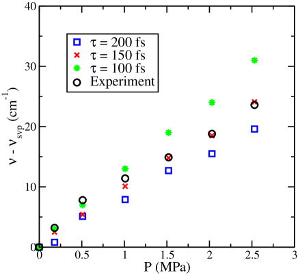
Figure 26: Pressure induced shift for the He^∗ (1s2p) $\leftarrow$(1s2s) absorption line in superfluid helium.Fie14 Comparison between the calculated line shifts (OT-DFT and Eq. (65)) for selected values of the dephasing time constant $\tau$ and the experimental data obtained at 1.6 K temperature.Hic75 ; Sol74

The above line shape model has also been employed to calculate He^∗ (1s3s) $\rightarrow$ (1s2p) and He${}^{*}_{2}$ ³d $\rightarrow$ ³a fluorescence line shifts as a function of pressure.Bon12 ; Bon16 In general, the calculations show slightly larger blue shifts than the experimental data, which may be related to the higher temperature in the experiments vs. calculations or to the accuracy of the used He^∗-He and He${}^{*}_{2}$-He pair potentials. Note that the experimental line shifts are sensitive to energy differences of just a couple of cm^-1 far away from the impurity.

Finally, we mention a time-dependent OT-DFT calculation modelling the superfluid dynamics following a two-photon excitation of the He${}^{*}_{2}$ excimer from the ³a to the ³d state.Elo07 These calculations, which were carried out in 1D spherical coordinates, were motivated by earlier optical pump-probe measurements that determined the bubble breathing period around the ³d state as a function of $P$ and $T$.Ben02 The period was observed to track the bulk liquid viscosity and reached ca. 150 ps at the lowest measured temperature of 1.4 K. The normal fluid fraction at this $T$ is only 0.08, which implies that the viscous contribution to the breathing period should be very small. While the OT-DFT calculations carried out in Ref. Elo07, did not include this viscous response, bubble breathing periods in the range of 50 to 120 ps were obtained depending on the He${}^{*}_{2}$-He potential employed. Two open questions still remain regarding this system: 1) inclusion of the viscous response [see Eq. (69)]; and 2) accurate calculation of the long-range He${}^{*}_{2}$(³d)-He interaction potential. The latter may also require inclusion of many-body corrections beyond the pair potential approximation as the ³d Rydberg orbital is somewhat compressible.Elo01

V.9 Translational motion of ions below the Landau critical velocity

In addition to the above mentioned solvation dynamics of ions in superfluid helium, the hydrodynamic response of the surrounding liquid due to translational motion of various ions has been studied by OT-DFT.Fie12 ; Mat15b At $T=0$, provided that the ion velocity remains well below the Landau critical value, dissipation of energy can only take place through the emission of sound when the ion accelerates or decelerates in the liquid. In the presence of thermal excitations (i.e. thermal phonons and rotons), the viscous drag force also opposes the ion motion. The most important experimentally accessible parameters that are sensitive to this dissipative liquid response are the ion hydrodynamic mass $(m_{add})$ and the ion mobility ($\mu$). The former quantity corresponds to the difference between the bare ion mass in vacuum and its effective mass in the liquid whereas the ion mobility is determined by the ion steady-state velocity in the liquid.Bor07

Hydrodynamic added masses for several halogen anionsFie12 as well as bare positive (i.e. He${}_{3}^{+}$) and negative chargesMat15b in superfluid ⁴He have been calculated by OT-DFT. In the latter work, the ion mass was computed by imaginary-time OT-DFT in the co-moving reference frame (see also Sec. V.6)

$$\left[\hat{H}-v_{0,z}\,\hat{P}_{z}\right]\Psi(\mathbf{r})=\mu\,\Psi(\mathbf{r})$$ (67)

where $v_{0,z}$ is the constrained liquid velocity along the $z$-axis and $\hat{P}_{z}$ is the $z$-component of the momentum operator. An estimate for the added mass during imaginary-time iterations can be computed from

$$\frac{m_{add}}{m_{4}}=\frac{1}{v_{0,z}}\int d\mathbf{r}\,\rho(\mathbf{r})\,v_{z}(\mathbf{r})$$ (68)

where $v_{z}$ is the $z$-component of the liquid velocity $\mathbf{v}(\mathbf{r})=\mathbf{j}(\mathbf{r})/\rho(\mathbf{r})$. This model yields results consistent with the available experimental information (i.e. positive and negative charges)Mat15b as well as the independently obtained QMC data (i.e. K⁺).Fie12 ; Buz01

In ion mobility experiments, an external electric field accelerates the ion until the electrostatic and hydrodynamic drag forces cancel. The resulting steady-state velocity $v_{z}$ is directly related to the ion mobility, $\mu=ev_{z}/F_{z}$, where $F_{z}$ is the electrostatic force acting on the ion. In a liquid at $T\neq 0$, the drag force arises from collisions with thermal excitations, whereas in the limit of 0 K the ion could in principle accelerate until the critical value for the creation of vorticity or turbulence is reached (see Sec. V.6 for the case of an electron).

To help comparison with the available experimental mobility data,Bor07 the standard OT-DFT functional must be extended to include the liquid viscous response. At temperatures higher than 1.4 K, the roton density is sufficiently high for a continuum-based model to be applicable. The viscous response term from the Navier-Stokes equation can be adapted to DFT by employing the Madelung transformation,Ait16 see also Sec. IV.2. This gives the following equation for the associated non-linear potential, $V_{NS}=V_{NS}\left[\rho,\textbf{v}\right]$,

$$\nabla^{2}V_{NS}=-\nabla\cdot\left\{\frac{1}{\rho}\left[\eta\left(\nabla\mathbf{v}+\left(\nabla\mathbf{v}\right)^{\rm T}-\frac{2}{3}\left(\nabla\cdot\mathbf{v}\right)\mathbf{1}\right)\right]\right\}$$ (69)

where $\eta=\eta(\rho,T)$ is the liquid shear viscosity, $\mathbf{1}$ denotes the unit tensor, and superscript T denotes matrix transpose. Note that this form allows for both liquid compression ($\nabla\cdot\mathbf{v}\neq 0$) and rotation ($\nabla\times\mathbf{v}\neq 0$) as well as spatial variation of the viscosity. The discrete form of this equation reduces to the Poisson problem, which can be efficiently solved in Fourier space using standard techniques.Pre92

An additional complication arises from the presence of a wide gas-liquid interface surrounding most ions in superfluid helium. To obtain agreement with the experimental electron mobility data, the shear viscosity in this region must be modified from the bulk value, $\eta\left(\rho(\textbf{r}),T\right)=\left[\rho(\textbf{r})/\rho_{0}(T)\right]^{\alpha(T)}\eta_{0}(T)$.Ait16 where $\alpha(T)$ determines the spatial variation of the viscosity across the interface and $\eta_{0}$ is the bulk shear viscosity.

The steady-state liquid flow solution around the ion can be obtained by including Eq. (69) in the OT functional and propagating the system in imaginary-time according to the velocity constraint of Eq. (67). Under this condition, the electrostatic and drag forces cancel out and the ion mobility can be evaluated. The hydrodynamic drag on the ion can simply be obtained by calculating the force due to the surrounding liquid for classical impurities (see Eq. (47)). If the impurity (e.g. electron) is treated quantum mechanically, integration over the impurity coordinate must also be included. This model was shown to reproduce the known electron mobility data between 1.4 K and the lambda point along the saturated vapor pressure line.Ait16 As an illustration, Fig. 27 shows the results for an electron moving in superfluid helium at 2.1 K.

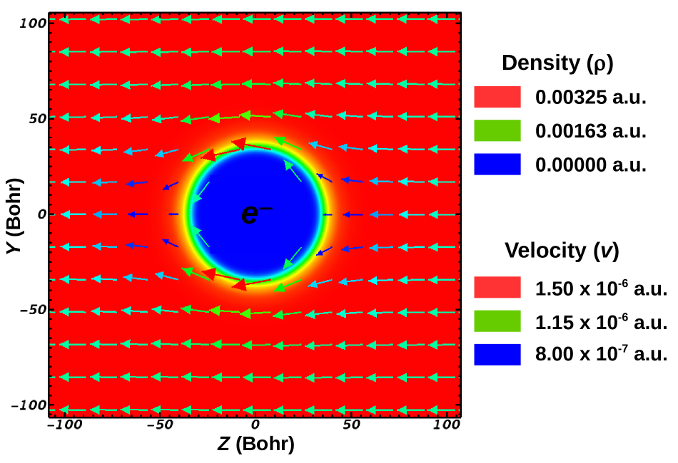
Figure 27: Steady-state helium density contours ($\rho$) and velocity field ($v$) around an electron moving in superfluid helium at $T=2.1$ K. The velocity component shown along the $z$-axis was shifted by $v_{0}=-2.3$ m/s.Ait16

V.10 Critical Landau velocity in small ⁴He droplets

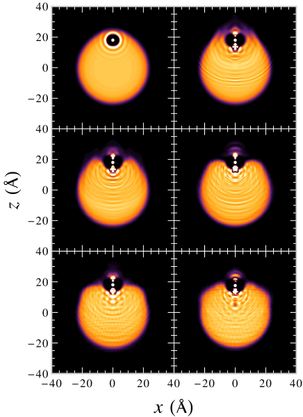
Figure 28: Dynamic evolution of an Ag@⁴He₁₀₀₀ complex upon sudden excitation of Ag to the ²P_3/2 state displaying the appearance of a linear AgHe₂ exciplex on the droplet surface. The Ag atom is initially at rest 18 Å off the center of the droplet. Snapshots are shown every 4 ps starting from the top left frame.Mat13b

Many properties of helium nanodroplets have been characterised during the last two decades by using solvated molecules as spectroscopic probes. In particular, vibrational and rotational spectroscopy of solvated carbonyl sulfide (OCS) provided evidence for microscopic superfluidity in these finite size systems.Toe04 ; Gre98 However, this raises the question to what extent can microscopic superfluidity be related to the frictionless flow of superfluid helium.

The first point considered was the existence of Landau critical velocity in helium nanodroplets, which are microscopic objects of only 10³-10⁶ atoms, and the possibility of using atoms or molecules as probes for it. This was the starting point of a joint experimental and theoretical searchBra13 for the existence of a limiting velocity for species ejected from helium droplets.

The following scheme was designed for that purpose. A probe atom or molecule, initially located in the bulk portion of the droplet, was suddenly optically excited to an electronic state with repulsive interaction with helium. As a consequence, the probe is accelerated and ejected from the droplet. If there is a critical velocity, the probe cannot accelerate beyond it and this will be reflected in its final velocity. Experimental measurements of the velocity distributions of atoms/molecules ejected from various size helium droplets have revealed the existence of a critical velocity threshold even for droplets consisting of a thousand helium atoms. In particular, ²P_1/2 excitation of Ag leads to its ejection with a velocity distribution peaking around 55 m/s. A similar, although not identical, velocity distribution was obtained upon excitation to the ²P_3/2 state, where the ejected species was either Ag or AgHe. DFT simulations on the dynamic evolution of this systemMat13b ; Lea16 confirmed these findings and provided additional microscopic details of the process. In particular, running the simulation for several tens of picoseconds was sufficient to observe the AgHe exciplex formation as shown in Fig. 28.

V.11 Rotational superfluidity

Superfluidity of helium droplets has been extensively studied by both experiments and theory.Bart96 ; Toe98 ; Gre00 As discussed earlier, previous experimental work has employed molecular probes to interrogate the droplet response to both radial and rotational excitation.Har96 ; Jag02 While these experiments have demonstrated the presence of the characteristic roton energy gap for larger droplets (i.e. the Landau criterion for superfluidity), microwave spectroscopy experiments indicated that non-classical behavior already takes place in molecule-helium clusters with less than ten He atoms.Jag02 In these experiments, the rotational constant $B$ (proportional to the inverse of the moment of inertia) was determined as a function of the number of helium atoms in the cluster. $B$ was observed to initially decrease with $N_{4}$ as expected for a classical rotor, but then it started increasing again from a given size on, which depended on the probe,Jag03 ; Jag07 ; Jag08 as shown in Fig. 29. This turning point has been interpreted as the onset of superfluidity in small helium droplets ($N_{4}<20$).Jag02 It seemed to contradict the original Laudau criterion for superfluidity since previous QMC calculations had shownSin89 ; Kro01 that there was no roton energy gap in droplets with less than ca. 64 ⁴He atoms.

Recent OT-DFT calculations employing the rotational constraint of Eq. (31) have resolved this discrepancy by identifying the quantum mechanical origin of the non-classical reduction in rotational friction.Mat15b The only input to this model is the probe molecule-He interaction, i.e. the external potential for OT-DFT, taken from ab initio electronic structure calculations. The rotationally constrained OT-DFT equation was solved by the ITM, which yielded the stationary order parameter $\Psi$ with the associated liquid density and velocity field rotating with the molecule. The added moment of inertia for the rotor ($I_{add}$), which is equivalent to $m_{add}$ for translation motion, can be computed from

$$I_{add}=\left<\Psi|L_{z}|\Psi\right>/\omega$$ (70)

where $\hat{L}_{z}$ is the $z$-component of the liquid angular momentum operator and $\omega$ is the frequency of rotation – typically less than 1 GHz; see Eq. (31). The effective rotational constant of the molecule in superfluid helium, $B_{eff}$, is then given by

$$B_{eff}=\frac{\hbar}{4\pi c\left(I_{gas}+I_{add}\right)}$$ (71)

where $I_{gas}$ is the moment of inertia of the molecule in the gas phase.

Four different probe molecules, which can be classified as ‘heavy’ or ‘light’ rotors based on their gas phase moments of inertia, were studiedMat15b (see Fig. 29). The results showed that the experimentally observed turning points in the $B(N_{4})$ curve correlated with helium coverage of the probe molecule. When a connected path of helium forms around the molecule, helium attempts to remain irrotational by introducing negative angular momentum to decouple from the rotational motion. This explains why the position of the turning point depends on the probe molecule itself. In addition, this turning point correlates with the appearance of a continuous helium coverage around the probe rather than the completion of the first solvation shell. Secondary oscillations in $B(N_{4})$ were related to the complete coverage of the subsequent helium layers.

The appearance of global phase coherence around the probe molecule produces a Landau-type energy gap between the droplet rotational ground and first excited states. This gap plays a similar role for rotational motion as the Landau roton gap in traditional superfluidity. When analysed in the co-rotating frame of reference, the transition bears similarities to the Mott-1D superfluid quantum phase transition.Gre02 In order to distinguish this phenomenon from the traditional translational superfluidity, we refer to it as rotational superfluidity.Mat15b

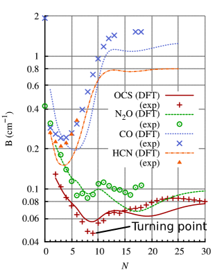
Figure 29: Experimental (exp) and calculated (DFT) effective rotational constants as a function of helium droplet size. The position of the non-classical turning point for OCS is indicated by a line.Mat15b

V.12 Interaction of impurities with vortex lines

Much of what is known on vortices in helium has been drawn using ions and electrons as probes in experiments. In this section we present results for ions, electrons, and neutral impurities obtained by static DFT calculations and leave the discussion of dynamical capture of impurities by vortices in helium dropletsCop17 to Sec. V.15. The reader should note the different sign convention for the binding energy of an impurity to the vortex line used in the following Secs. V.12.1 and V.12.2. We have kept the convention used in the original papers.

V.12.1 Electrons

DFT calculations can provide detailed information about electron trapping on quantised vortex lines.Pi07 The degenerate electronic states (e.g. p, d, f $\ldots$) of the bubble split if the bubble becomes non-spherical. For this reason, when the electron bubble becomes trapped on a vortex line, the resulting symmetry breaking leads to the splitting of the energy levels. Provided that this splitting is large enough, it could be observed by absorption spectroscopy.

The absorption spectrum of the electron bubble can be obtained from the dipole strength function $S(\omega)$

$$S(\omega)=\sum_{n\neq 0}|\langle n|\mathbf{r}|0\rangle|^{2}\delta(\omega-\omega_{n0})$$ (72)

where $|0\rangle$ and $|n\rangle$ correspond to the ground and excited states of the electron bubble, respectively. The infrared absorption spectrum of the e-bubble from DFT calculations is shown in Fig. 30 in the range of 1s–1p and 1s–2p transitions. The function $S(\omega)$ displays peaks centered at the absorption energies $\omega_{n0}$. Furthermore, the figure shows that the effect of vortex trapping on the absorption spectrum is very small, especially for the 1s–1p transition. Slightly larger changes are observed for the 1s–2p transition, which originates from the more pronounced penetration of the 2p electron wave function into the liquid. However, this transition is much weaker than the 1s–1p one. Based on these results, it can be concluded that the infrared absorption spectrum of the e-bubble is not very sensitive to the possible vortex trapping and hence, it is not generally suitable for detecting vorticity.

The 1p–1s emission energy has been calculated for both free and vortex trapped e-bubbles.Mat10b This calculation assumes that the radiative lifetime of the excited state is longer than the time required for the liquid to equilibrate around the electron. Experimental data indicate that the radiative lifetime is some tens of nanosecondsGho05 or even tens of microseconds when calculated directly from the transition dipole moment.Leh07 Based on the simulations, the equilibrium geometry around 1p is reached after several hundreds of picoseconds.

Figure 30: Dipole strength $S(\omega)$ (arbitrary scale) at $P=T=0$ for a spherical electron bubble (solid line) and for an electron bubble attached to a linear vortex (dashed line). The inset shows $S(\omega)$ in logarithmic scale.Mat10b

The most important quantity that can be extracted from the calculations is the binding energy of the e-bubble to the vortex line. This can be obtained from the grand potential per unit volume, $\Omega\equiv(F-\mu_{4}N_{4})/{\cal V}$, for e-bubble configurations with and without a vortex line at the same temperature and pressure:

$$B_{e-V}=[\Omega_{e}-\Omega]-[\Omega_{e+V}-\Omega_{V}]$$ (73)

where the subscripts refer to vortex-free e-bubble ($e$), bulk liquid (none), e-bubble attached to a vortex line ($e+V$), and vortex line alone ($V$). Since all the terms above are evaluated under the same thermodynamic conditions, their chemical potential $\mu_{4}$ and the saturation liquid density are identical. The above expression is therefore well-defined and independent of the simulation box volume. Alternatively, one may use the substitution energy introduced in Sec. III.2, which differs from the value of Eq. (73) by ca. 10%. The calculations yield the electron binding energy as $B_{e-V}=104.5$ K at $P=T=0$, which shows that trapping of electron bubbles on vortex lines is energetically very favored. A value of 109 K was found in Ref. Mat15a, ; the difference between the two values is attributed to the different electron-helium interactions used.

The attractive interaction between an electron and a vortex line can be understood in terms of the loss of kinetic energy due to the liquid displaced by the approaching electron bubble (i.e. the classical Bernoulli force).Bor07 The experimentally obtained values for electron binding to vortex lines vary between 55 and 59 K at $T=1.6$ K,Pra69 ; DeC74 ; Don91 which is in clear disagreement with the value obtained from OT-DFT calculations at $T=0$. Since this rather deep binding value is consistent with the large radius of the electron bubble,Gri92 ; Gra06 ; Cla98 ; Elo02 the difference has been attributed to the $T$ dependence of the vortex core parameter and local thermal deformations of the vortex line rather than to a deficiency in the OT-DFT-based model itself.Mat15a ; Pi07 ; Pad72 Furthermore, the same OT-DFT model is able to reproduce the experimental binding energy of positive charges (i.e. He${}^{+}_{3}$, Ref. Mat15c, ) to vortex lines: 16 K (calculated at 0 K) vs. 17.5 K (experiment at 0.3 K).Mat15a Once the thermal effects for the electron are taken into account, the OT-DFT binding energy is lowered down to 61 K, which is very close to the experimental estimates.Mat15a Thus, vortex lines present very deep traps for electrons in superfluid helium.

V.12.2 Atomic and molecular impurities

Just as electrons trap on vortex lines, any impurity should be attracted towards them due to the Bernoulli force. Given a sufficiently high concentration of neutral impurities in the liquid, they can accumulate on vortex lines as a consequence of this attraction. Subsequent diffusion along the vortex line may then lead to the assembly of nanowires, which are reminiscent of the original vortex line geometry. The final products from this process have been observed in metal doped bulk superfluid heliumGor14 ; Gor15 ; Pop13 and superfluid helium droplets.Gom12 ; Lat14 ; Spe14 One of the main factors influencing the initial stage of the nanowire assembly is the impurity-vortex line interaction, which has been modelled by OT-DFT calculations.Mat15a

Impurity		$R$		$a_{F}$	OT-DFT $V_{\textnormal{im-vortex}}$	Exp. $V_{\textnormal{im-vortex}}$
		(Å)		(Å)	(K)	(K)
H2 ($X$ ${}^{1}\Sigma_{g}$)		3.1		0.38	$-9.4$	–
Ag2 ($X$ ${}^{1}\Sigma_{g}$)		3.9		0.51	$-10.9$	–
Cu2 ($X$ ${}^{1}\Sigma_{g}$)		4.0		0.52	$-11.4$	–
Ag (${}^{2}S$)		4.4		0.63	$-12.0$	–
Cu (${}^{2}S$)		4.5		0.65	$-12.5$	–
He${}_{3}^{+}$ ($X$ ${}^{2}\Sigma_{g}$)		$\approx 5.7$		$\approx 0.75$	$-16.0$	$-17.5$ at 0.28-0.6 K, Refs. Ost75,; Wil75,
Li (${}^{2}S$)		6.8		0.75	$-21.5$	–
He∗ ($2s$ ${}^{3}S$)		7.1		0.77	$-22.6$	–
He${}^{*}_{2}$ ($a$ ${}^{3}\Sigma_{u}$)		8.6		0.80	$-29.8$	–
$e^{-}$ ($1s$)		22.2		0.76	$-109^{\;\rm a}$	$-55$ to $-59$ at 1.6 K, Refs. Pra69,; DeC74,

Table 3: Summary of the impurity-vortex interaction parameters at $P=T=0$ based on Eq. (75). $R$ represents the classical bubble radius for the impurity, $a_{F}$ is the healing length, and $V_{\textnormal{im-vortex}}(0)$ denotes the total binding energy.Mat15a ^a See discussion in Sec. V.6 regarding the value for the electron.

The actual impurity trapping event is clearly a dynamic process, see Sec. V.15. Assuming that the impurity impact velocity remains small and the vortex line geometry does not deviate from linear geometry, static interaction energy potentials for the vortex-impurity interaction can be obtained. This calculation can be carried out in imaginary-time where the vortex line structure is imposed by the initial guess given by Eq. (28). The position of the impurity must remain fixed during the calculation, which can be imposed by including the following penalty term in the external potentialMat15a (see also Eq. (24))

$$V[\Psi,\mathbf{r}]=2\,\lambda_{C}\,(z-z_{0})\int d\mathbf{r}^{\prime}\Psi^{*}(\mathbf{r}^{\prime})\,(z^{\prime}-z_{0})\Psi(\mathbf{r}^{\prime})$$ (74)

where $\lambda_{C}\sim 10^{-5}$ a.u., and the impurity is constrained along the $z$-axis (perpendicular to the vortex line) at position $z_{0}$. Calculation of the total energy of the system as a function of the distance between the vortex line and the impurity yields the static interaction potential.

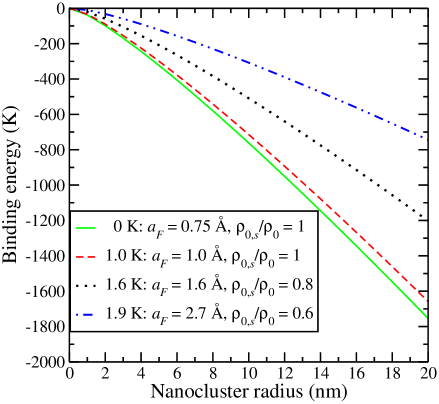
Figure 31: Nanocluster-vortex binding energies according to Eq. (75) as a function of the cluster size at indicated temperatures.Mat15a

In addition to providing the total binding energies of impurities to vortex lines, the interaction energies can be rationalised by the Donnelly-Parks potential functionPar66 (see also Eq. (29))

$$V_{\textnormal{im-vortex}}(r)=-2\pi\rho_{0,s}\left(\frac{\hbar^{2}}{m_{4}}\right)^{2}\int_{0}^{R}d\xi\frac{\left(R^{2}-\xi^{2}\right)^{1/2}\xi}{\left[\left(\xi^{2}+r^{2}+a_{F}^{2}\right)^{2}-4r^{2}\xi^{2}\right]^{1/2}}$$ (75)

where $R$ represents the classical radius for the spherical cavity containing the impurity, $r$ is the vortex core-impurity distance, $\rho_{0,s}$ is the bulk superfluid helium density, and $a_{F}$ is the effective healing length. Non-linear least squares fit of this expression to the interaction potential energy curves from OT-DFT provides effective size estimates for both $R$ and $a_{F}$. Some of the obtained results are shown in Table 3.

Nanowires in liquid helium are believed to form through recombination of metal nanoparticles in the vortex rather than through building up from individual atoms.Gor15 ; Vol16 The size of such particles is too large for any practical OT-DFT calculation. Therefore, the binding energy estimates for nanoparticles bound to rectilinear vortex lines can only be obtained from Eq. (75). Note that this assumes that the vortex lines are linear and longer than the diameter of the approaching nanoparticle. The binding energy data as a function of the nanoparticle radius is shown in Fig. 31. The effect of temperature was included in the estimate by varying the superfluid density ($\rho_{0,s}$) and the healing length ($a_{F}$) accordingly. While the binding energies quickly exceed 1000 K, under real experimental conditions this may rather be limited by the dimensions of the vortex line itself.

V.13 Vortex arrays in ⁴He droplets

Together with the frictionless motion of impurities at velocities below the Landau critical velocity in superfluid ⁴He, the appearance of quantised vortices is another signature of superfluidity. Helium remains at rest when its container is rotated, until a critical angular velocity is reached. This leads to the appearance of vortices with quantised velocity circulation in units of $h/m_{4}$, where $h$ is the Planck constant.

The vortex line distributions in superfluid ⁴He were first imaged by Williams and PackardWil74 by means of light scattered by electrons attached to the vortex lines; quantised vortices have also been visualised by suspending micron-sized solid particles of hydrogen in bulk superfluid ⁴He.Zha05 ; Bew06 More recently, femtosecond single-shot x-ray diffraction imaging of Xe doped ⁴He droplets employing a free electron laser, revealed Bragg spots confirming the existence of quantum vortex arrays in helium droplets.Gom14 ; Jon16 ; Ber17 This result shows that large ⁴He droplets containing about 10¹⁰ atoms are superfluid.

As discussed earlier, DFT has proven to be a very useful theoretical tool to study vortices in liquid ⁴He. In most recent applications, vortex arrays in a rotating ⁴He nanocylinderAnc14 and in ⁴He nanodropletsAnc15 were studied by DFT. In the former case, the $n_{v}$-vortex stability diagram was computed and compared with that of classical vortex lines in an inviscid, incompressible fluid. Vortex array configurations in a rotating cylinder – as that shown in Fig. 32 – can be completely characterised within the Onsager-Feynman model by the dimensionless energy per unit length ${\cal E}\equiv(m_{4}/\rho_{0}\pi\hbar^{2})E$, the dimensionless angular velocity $\Omega\equiv R^{2}m_{4}\,\omega/\hbar$, and the scaled radial positions of the vortices $r_{i}/R$. Here $\rho_{0}=0.0218$ Å^-3 is the bulk density and $R$ is the radius of the cylinder.Hes67 By scaling the calculated values to millimeter-scale, the nanoscale results agree with the experimental data on vortex arrays observed in the bulk liquid.Wil74

The appearance of vortex arrays in rotating ⁴He nanodroplets at $T=0$ was recently investigated by DFT.Anc15 The results were compared with the theory developed for rotating classical fluid spheres, which was earlier used to analyze the shape and vorticity in helium droplet experiments.Gom14 In agreement with the experimental data, the droplets remain stable well above the stability limit predicted by classical theories despite their large shape deformations due to rotation.Cha65 ; Bro80 Vorticity inside the droplets changes their appearance from ellipsoidal to oblate and ‘wheel’-shaped with small and large vortex densities, respectively. In agreement with the experiments, the latter shape exhibits nearly flat upper and lower surfaces. Selected vortex array configurations for a $N_{4}=15000$ droplet are shown in Fig. 33.

The above results can be compared with the experimental data obtained for much larger droplets once they are scaled by a dimensionless characteristic rotational velocity $\Omega$

$$\Omega=\sqrt{\frac{m_{4}\rho_{0}R^{3}}{8\,\gamma}}\,\omega$$ (76)

where $\gamma=0.274$ K Å^-2 is the surface tension of the liquid. For a $N_{4}=15000$ droplet, $\Omega=1$ corresponds to $\omega=1.13\times 10^{10}$ s^-1.

The data shown in Fig. 33 demonstrate that the rotating droplet aspect ratio – defined as $b/a$ where $a$ is the short half-axis and $b$ the long half-axis length – depends on the angular frequency. The calculated $b/a$ vs. $\Omega$ is plotted in Fig. 34 together with the classical model prediction, which was used in Ref. Gom14, to interpret the experimental observations. Notice the gaps that appear in the calculated data, which reflect the presence of forbidden values of the angular momentum per atom. Similar gaps have also been observed in calculations modelling trapped rotating BEC.But99 Despite the apparent differences between rotating classical and superfluid droplets, the relationship between the aspect ratio and the angular frequency looks very similar. The classical model underestimates the angular frequency only by less than 10% for large vortex arrays.

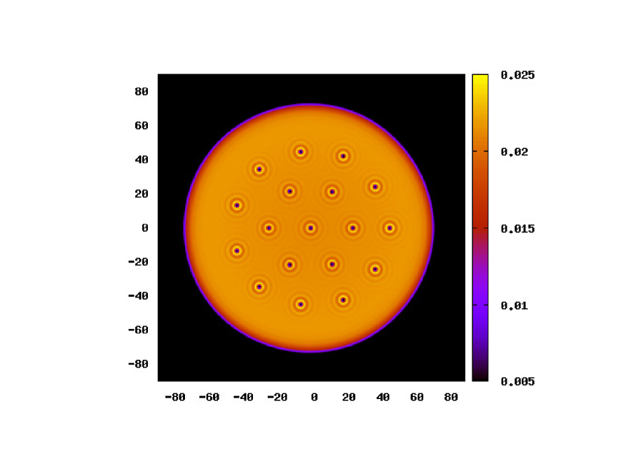
Figure 32: Lowest energy stationary 18-vortex configuration in a nanocylinder of $R=71.4$ Å radius at $\Omega=29.6$ (defined in Eq. (76)). Distances are specified in Å. The contour colors correspond to density values between $\rho=0$ and $\rho=0.03$ Å^-3.Anc14

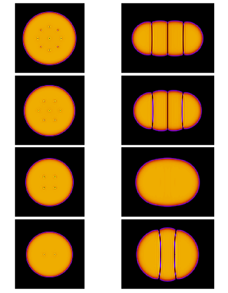
Figure 33: From bottom to top, helium droplet configurations hosting $n_{v}=$ 2, 4, 7 and 9 vortex lines. The left column shows the helium density on the $z=0$ symmetry plane (top view) and the right column on the $x=0$ plane (side view).Anc15

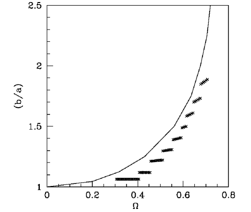
Figure 34: Aspect ratio $b/a$ as a function of the dimensionless angular velocity $\Omega$ [defined in Eq. (76)] for a $N_{4}=15000$ droplet. The solid line shows the experimental curve obtained by using the classical model. Discontinuities in $b/a$ vs. $\Omega$ appear at the values corresponding to phase transitions between configurations with different number of vortices (from 1 to 9).Anc15

The experimental diffraction images of Xe doped He droplets ($\sim$200 nm diameter) have revealed configurations made of symmetrically arranged vortex arrays that are decorated with Xe clusters at unexpectedly large distances from the centre of the droplet.Jon16 These observations have been explained in terms of angular momentum conservation. When the Xe atoms are drawn to the vortex cores, they start rotating along with the vortex array. The increased moment of inertia due to the additional Xe atoms must decrease the rotational angular velocity of the vortex array causing it to expand such that the inter-vortex distances increase. Note that the DFT results discussed above refer to pure helium droplets. Results for vortex arrays in helium nanocylinders that are decorated with Xe atoms are discussed in Ref. Anc14, .

The above system was recently modelled by DFT using Ar doped helium droplets because the calculations are technically simpler than for Xe.Cop17 The system considered consisted of an array of six vortex lines filled with Ar atoms inside a $N_{4}=15000$ droplet ($\sim$11 nm diameter). In qualitative agreement with the experimental observations, the calculations show that the doping of the vortex cores substantially increases the rigidity of the system. This, in turn, makes the droplet stable at lower angular velocities and increases the inter-vortex distances. In contrast, a pure helium droplet with the same vortex array would have been unstable and the vortices would have been expelled off the droplet. Moreover, the solvation potential effect – which tends to attract the Ar atoms towards the center of the droplet – becomes apparent since, below some critical value of the angular velocity, the vortices cease to displace towards the surface and the system reaches an equilibrium maximum distance of the vortices from the droplet centre.

V.14 Dynamics of alkali atoms excited on the surface of ⁴He droplets

In a quest to understand how chemical reactions proceed in ultra-cold helium droplets, real time dynamics of photoexcited and photoionised atoms and molecules have been studied extensively by TDDFT. These processes share some elements with condensed phase chemical reactions, namely the dynamic liquid rearrangement and strong coupling of the electronic degrees of freedom to the surrounding liquid.

Photodissociation of Cl₂ and the following relaxation dynamics in ⁴He droplets has been recently addressed.Vil15a ; Vil16a ; Vil15b These studies constituted the first application of TDDFT to describe photodissociation of a homonuclear diatomic molecule embedded in superfluid helium. Related processes experimentally studied include photodissociation of alkyl iodidesBra07a ; Bra07b ; Bra07c and Cr₂ molecules.Kau15 From the theory point of view, a major technical problem in modelling such systems is that a large amount of energy is deposited into the liquid. Unless the number of atoms in the droplet is very large (millions of atoms), the droplet is expected to disintegrate on a sub-picosecond time scale. Since large helium droplets can be approximated by the bulk liquid, theoretical calculations could be carried out in the bulk to avoid helium evaporation from the droplet surface. Irrespective of the geometry of the helium sample, these calculations require accurate dimer/molecule-helium interaction potentials, which poseses a challenge even to modern electronic structure methods.

The dynamics following photoexcitation of alkali atoms attached to helium droplets has been investigated in a series of joint experimental and theoretical works.Her12a ; Van14 Photoelectron spectroscopy revealed that, upon excitation from the ground to the first excited s-state, alkali atoms desorb from the droplet surface. The mean kinetic energy of these atoms, which can be detected by ion imaging, shows a linear dependence on the excitation energy. TDDFT calculations on these systems revealed that the desorption process is accompanied by the creation of highly non-linear liquid density waves in the droplet that propagate at supersonic velocities.

The test-particle method described in Sec. IV.2 was introduced in the context of optical excitation of Li and Na atoms – sitting on the surface of helium droplets – to their first excited s-state.Her12a The ejected alkali metal atoms acquire high velocities, which makes the direct numerical solution of the Schrödinger equation difficult in the TTDFT context. An overview of the time evolution of the Na@⁴He₁₀₀₀ complex following the 4s $\leftarrow$ 3s excitation is shown in Fig. 35.Her12a The sudden repulsive interaction between the excited Na atom and the droplet creates a series of supersonic shock waves in the droplet, which indicates that a significant fraction of the energy introduced by the optical excitation is transferred directly into the droplet. These waves were observed to travel at velocities ranging from 370 to 890 m/s, which are of similar magnitude as recently observed in laser ablation experiments in the bulk liquid.Gar16 Furthermore, the moving high density peak, which originates from the first solvation shell, exhibits (bright) solitonic features such as constant propagation velocity (ca. 590 m/s) and no spatial dispersion. A similar result was found for the ejection of Rb and Cs atoms from helium droplets when excited from 5s to 6s and from 6s to 7s states, respectively.Van14

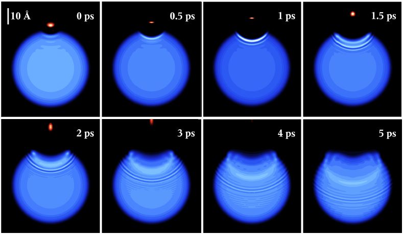
Figure 35: Time evolution of the Na@⁴He₁₀₀₀ complex upon 4s $\leftarrow$ 3s excitation.Her12a

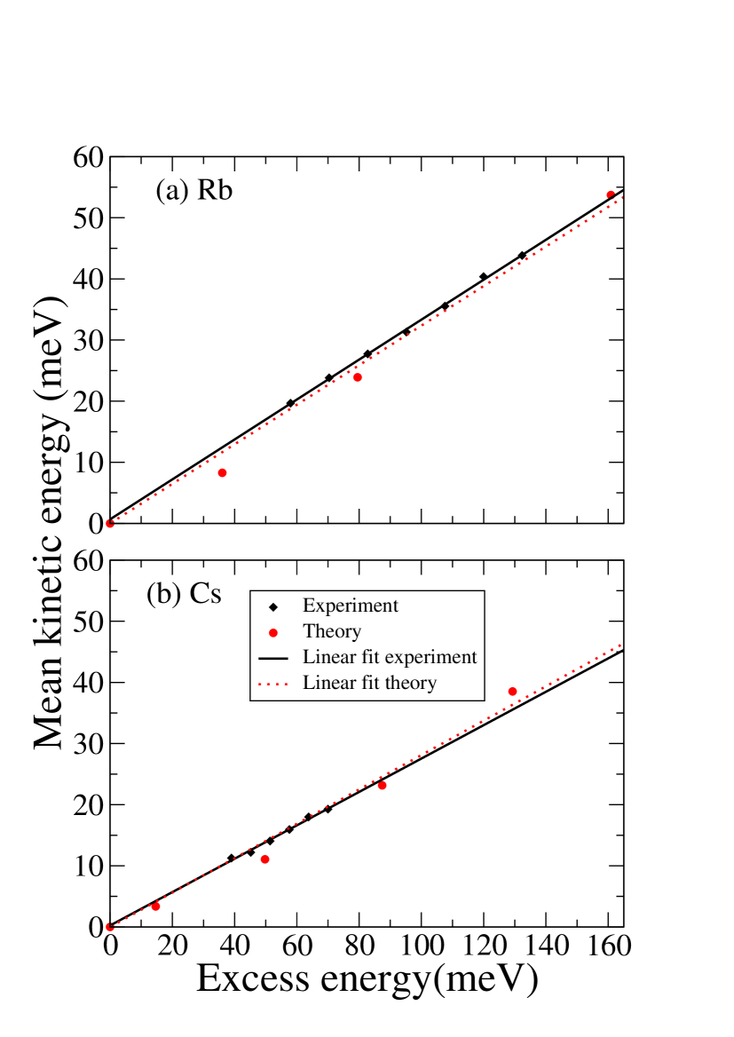
Figure 36: Mean kinetic energies of Rb (a) and Cs (b) atoms desorbing from helium droplets upon 6s$\Sigma$ and 7s$\Sigma$ state excitation, respectively. Straight and dotted lines: linear fits to the experimental and theoretical data, respectively.Van14

Detailed information about the kinematics of the process can be obtained by monitoring the kinetic energy of the atoms desorbed from the droplets as a function of the excitation energy.Her12a ; Van14 The experimental results for Cs and RbVan14 are shown in Fig. 36. The calculated points in that figure were obtained by starting TDDFT simulations from various impurity positions determined by a constrained minimization of the total energy of the complex. Whereas the light alkali metal atoms (Li and Na) require the use of the test-particle method, heavy alkali metals (Rb and Cs) can be treated classically.

For all alkali metals, the kinetic energy of the ejected atom exhibits a linear dependence on the excess excitation energy of the $(n+1)$s $\leftarrow$ $n$s transition. This indicates that, despite its apparent complexity, the ejection process can be well represented by a ‘pseudo-diatomic model’Bus72 in which the droplet is represented by one big atom bound to the alkali. By imposing energy and linear momentum conservation during the instantaneous ejection of the alkali atom from the droplet, the relative kinetic energy can be written as

$$E_{kin}=\eta(\hbar\omega-\hbar\omega_{0})\;,$$ (77)

where $\omega$ denotes the excitation and $\omega_{0}$ the atomic transition frequencies. The slope $\eta$ is related to the effective mass of the helium droplet (the mass of the helium atoms effectively participating in the interaction with the alkali atom), $m_{\mathrm{eff}}$, by

$$\eta=\frac{m_{\mathrm{eff}}}{m_{\mathrm{eff}}+m_{\mathrm{Ak}}}\Longrightarrow m_{\mathrm{eff}}=\frac{\eta}{1-\eta}\,m_{\mathrm{Ak}}\;.$$ (78)

Fitting the experimental and simulation data to Eq. (77) yields the results summarised in Table 4. It can be seen that $m_{\mathrm{eff}}$ increases with the mass of the alkali atom as indicated by Eq. (78). The variation of the corresponding number of helium atoms reflect the differences in the dimple structure and the excited state interaction with the droplet.Van14 Note the lack of data for the 5s $\leftarrow$ 4s transition for the K atom. While there is no difficulty in simulating it with TDDFT, this transition may overlap with 3d $\leftarrow$ 4s and this complicates the analysis of the experimental results.

Ak	mAk (exp)	$\eta$ (exp)	$\eta$ (th)	meff (exp)	meff (th)
	[amu]			[amu]	[amu]
Li	6.94	0.687	0.756	15.2	21.5
Na	23.0	0.516	0.583	24.6	32.2
Rb	85.5	0.327	0.324	41.9	41.0
Cs	132.9	0.281	0.273	51.8	50.5

Table 4: Some characteristics of the experimental and theoretical kinetic energy distributions of the desorbed alkali atoms;Her12a ; Van14 see text for details.

In addition to the $(n+1)$s $\leftarrow$ $n$s transitions discussed above (see also Refs. Log11a, ; Log11b, ; Pif10, ; Lac11, ), the lower energy $n$p $\leftarrow$ $n$s transitions have also been addressed in a series of experimental and theoretical studies.Sti96 ; Reh97 ; Bue07 ; Aub08 ; Lei08 ; Her10 ; Nak01 The first expectation was that alkali metal atoms would always detach from the droplets upon $n$p $\leftarrow$ $n$s excitation. However, only the light alkali metals such as Li, Na, and K appear to detach; the heavier alkalis (Rb and Cs) may remain attached if they are excited with energies close to that of the D1 line in the gas-phase.Aub08 ; The11

Photoexcitation and photoionisation of Rb atoms attached to helium droplets has been studied in real-time dynamics experiments.Van15 It was shown that excitation of Rb atoms from the 5s to the 6p states leads to their detachment. Upon subsequent ionisation of the excited Rb atom (Rb^∗), the interaction with helium becomes attractive. Hence, depending on the time delay $\tau_{D}$ between the excitation and ionisation laser pulses, the resulting ion may be ejected as a bare Rb⁺ cation or as a Rb⁺He_n complex, or it can be drawn into the droplet. The critical time $\tau_{c}$ separating these processes is called the fall-back time.Van15

Recently, this study has been extended to the Rb 5p $\leftarrow$ 5s transition.Van17 Both transitions have been simulated with TDDFT as described in Sec. IV.1. The Rb atom located on the droplet surface is first photoexcited to either the 5p or the 6p state (${}^{2}\Sigma_{1/2}$, ${}^{2}\Pi_{1/2}$ or ${}^{2}\Pi_{1/2}$) and the system evolves on the excited state potential energy surface. After a fixed delay, Rb^∗ is photoionised, which is simulated by suddenly switching the interaction potential to Rb⁺-He. It was found that the desorption process for the 6p state is impulsive whereas the behavior of the 5p state is intermediate between impulsive and complex dissociation. The desorption time scales are also very different for the two states: $\sim 1$ ps for 6p and $\sim 100$ ps for 5p.

Figure 37: Velocity of the Rb^∗ atom in the 5p ${}^{2}\Sigma_{1/2}$ and 5p ${}^{2}\Pi_{1/2}$ states (dashed lines) and the Rb⁺ cation produced by photoionisation (solid lines) after a given delay time vs. delay time. The fall-back times $\tau_{c}$ are indicated by arrows.

The velocities of Rb^∗ and the Rb⁺ as a function of the delay time are shown in Fig. 37 for the 5p $\leftarrow$ 5s transition. Note that the largest (asymptotic) velocity of Rb⁺ is simply given by the corresponding asymptotic velocity of Rb^∗ because the ion escape velocity is not affected by the droplet at large distances. TDDFT simulations have also been extended to the desorption of Cs following the 6p $\leftarrow$ 6s excitation.Cop17b The general features of the dynamics appear very similar to Rb 5p $\leftarrow$ 5s.

The TDDFT simulations for Rb and Cs atoms excited from their $n$s ground to their $n$p excited state can be summarised as follows: i) excitation to the ${}^{2}\Sigma_{1/2}$ or ${}^{2}\Pi_{1/2}$ state leads to desorption of the excited alkali atom (Ak^∗); ii) excitation to the ${}^{2}\Pi_{3/2}$ state produces an exciplex within $\sim$ 10 ps, which remains attached to the droplet surface.

Experiments and TDDFT calculations agree on the ejection of Ak^∗ ${}^{2}\Sigma_{1/2}$ state from helium droplets. At first sight, the results for ${}^{2}\Pi_{3/2}$ and ${}^{2}\Pi_{1/2}$ states seem to disagree with the experiments,Aub08 ; The10 ; The11 but this may be explained as follows.Bar17

$\bullet$ In the case of the ${}^{2}\Pi_{1/2}$ state, the experiments have explored the low energy region of the D1 line whereas the TDDFT dynamics was initiated using a configuration that corresponds to the D1 resonance. Hence, the initial energy in the TDDFT simulation is larger than in experiments.

$\bullet$ In the case of the ${}^{2}\Pi_{3/2}$ state, it is worth stressing that the electronic state of the ejected Ak^∗ was not determined in the experiments. Only the state to which the Ak atom was excited is determined (by the excitation laser wavelength). In the case of Rb^∗, experimental indications point to a non-radiative relaxation of the 5p${}^{2}\Pi_{3/2}$ to the 5p${}^{2}\Pi_{1/2}$ state.Van17 If this happens, the relaxed state may be a RbHe ${}^{2}\Pi_{1/2}$ exciplex. The energy available from this relaxation process is about 190 cm^-1. If even only one third of this energy is given to the RbHe ${}^{2}\Pi_{1/2}$ exciplex as additional initial kinetic energy, it is ejected from the droplet according to the TDDFT simulations. This process is compatible with the possibility of forming exciplexes in the ${}^{2}\Pi_{3/2}$ state which could remain attached to the dropletGie12 if no electronic relaxation occurs. Note that no exciplex was produced upon direct ${}^{2}\Pi_{1/2}$ excitation because of a barrier preventing its formation. A similar relaxation process is also fully compatible with the experimental observations for Ag.Mat13b

In a related study, DMC calculations have been carried out for Rb^∗ in a small cluster or on a helium film, which can be considered as a simplified model of a large droplet surface.Lei08 This study found that Rb^∗ stabilizes as a weakly bound metastable Rb ${}^{2}\Pi_{1/2}$ (not an exciplex) that forms a shallow dimple structure on the surface. There is no contradiction between the DMC and the dynamic TDDFT calculations in this respect: The DIM potentials indeed display a shallow minimum for this state so that the imaginary-time DFT relaxation would also yield a weakly bound Rb^∗. However, the energy available in the real time dynamics hinders the formation of this relaxed, weakly bound state. The same group later investigated Rb excited to the ${}^{2}\Pi_{3/2}$ state,Lei11 showing the appearance of a linear exciplex to which more helium atoms are attached, preferentially on one end of the linear exciplex. The TDDFT simulations are in agreement with these findings that, to a large extent, can be understood by inspecting the $V_{\lambda}$ DIM potentials, Eq. (44), as plotted in Fig. 38. Notice for example the appearance of two deep wells in the ${}^{2}\Pi_{3/2}$ potential; the filling of these wells by helium atoms yields the Rb₂${}^{2}\Pi_{3/2}$ linear exciplex.

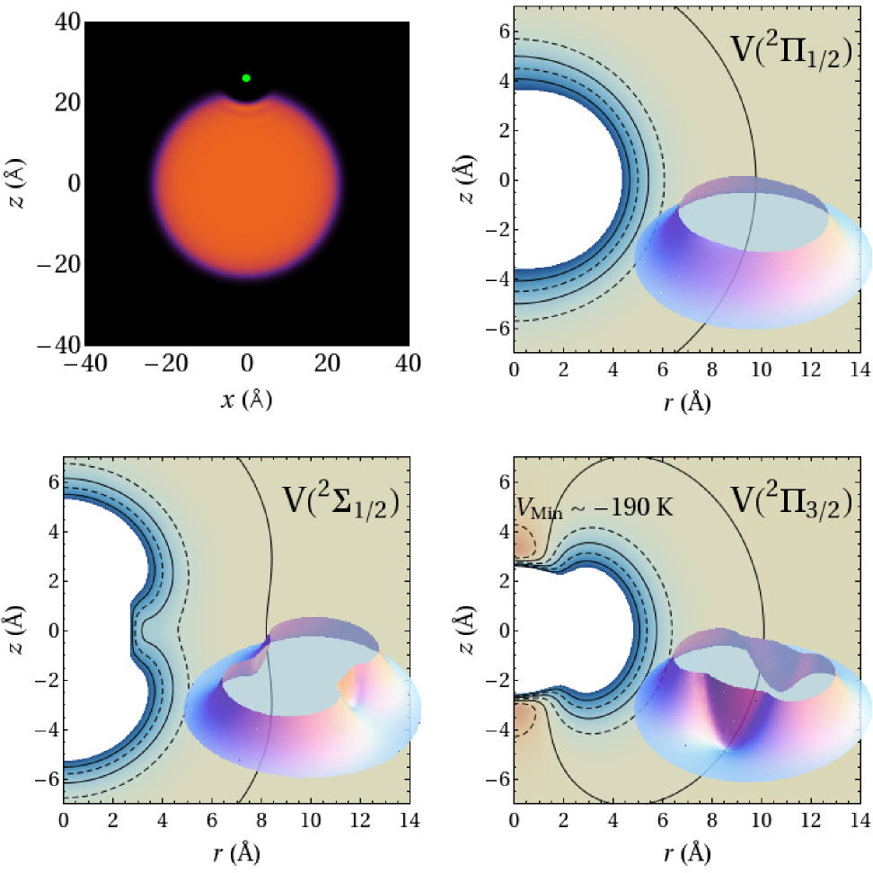
Figure 38: Top left panel: Equilibrium dimple configuration of Rb taken as starting point for the dynamics; the Rb atom is at 26.3 Å from the COM of the droplet. The other panels display the ²P $V_{\lambda}$ 5p Rb-He potentials (Eq. (44)) corresponding to this configuration. Regions where the potentials are attractive (repulsive) are represented in brown (blue). The outermost equidensity line corresponds to zero potential. The 5p ${}^{2}\Sigma_{1/2}$ and 5p ${}^{2}\Pi_{1/2}$ potentials have a shallow attractive minimum of about 1 K depth at a distance of $\sim$10 Å.

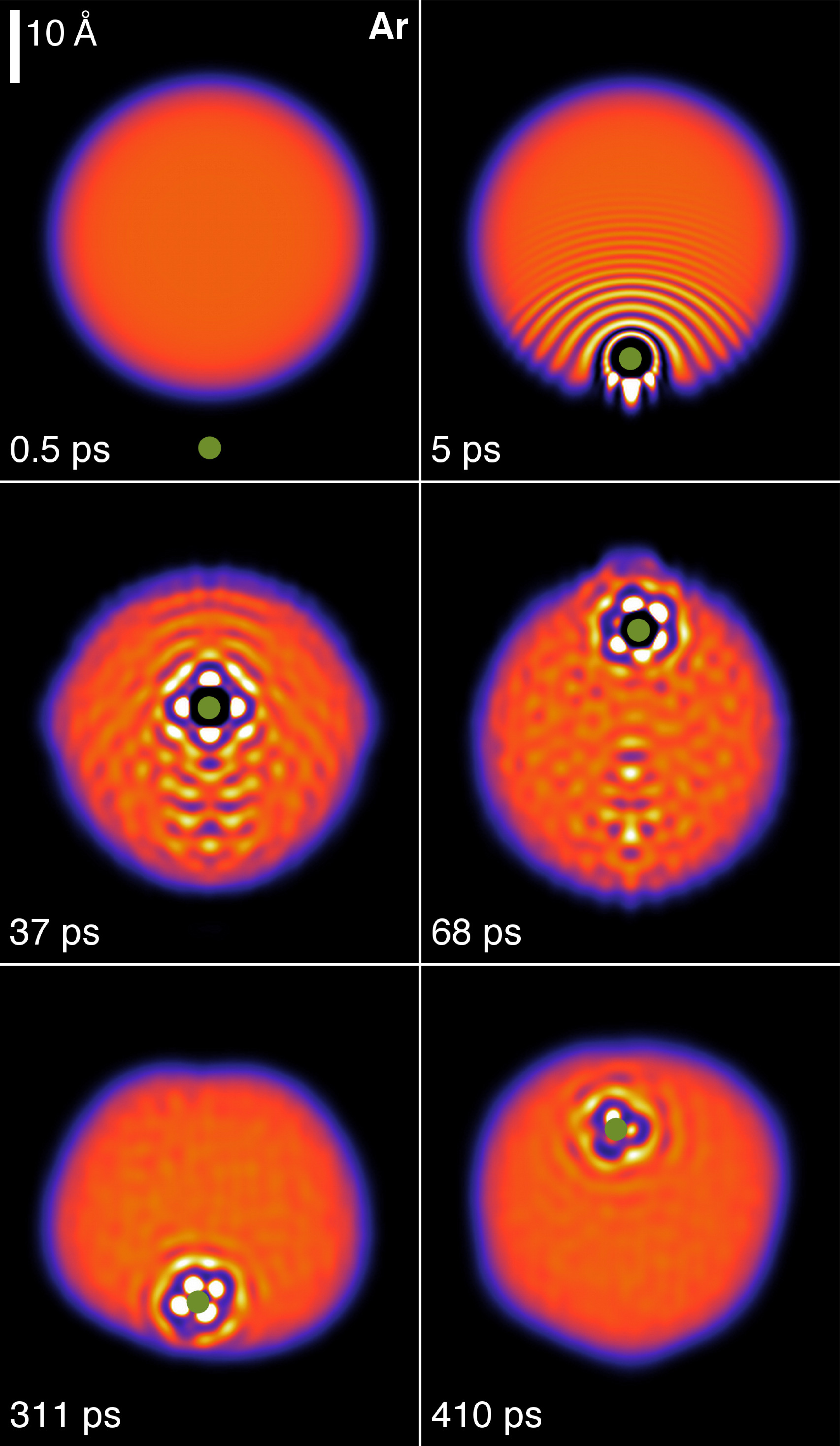
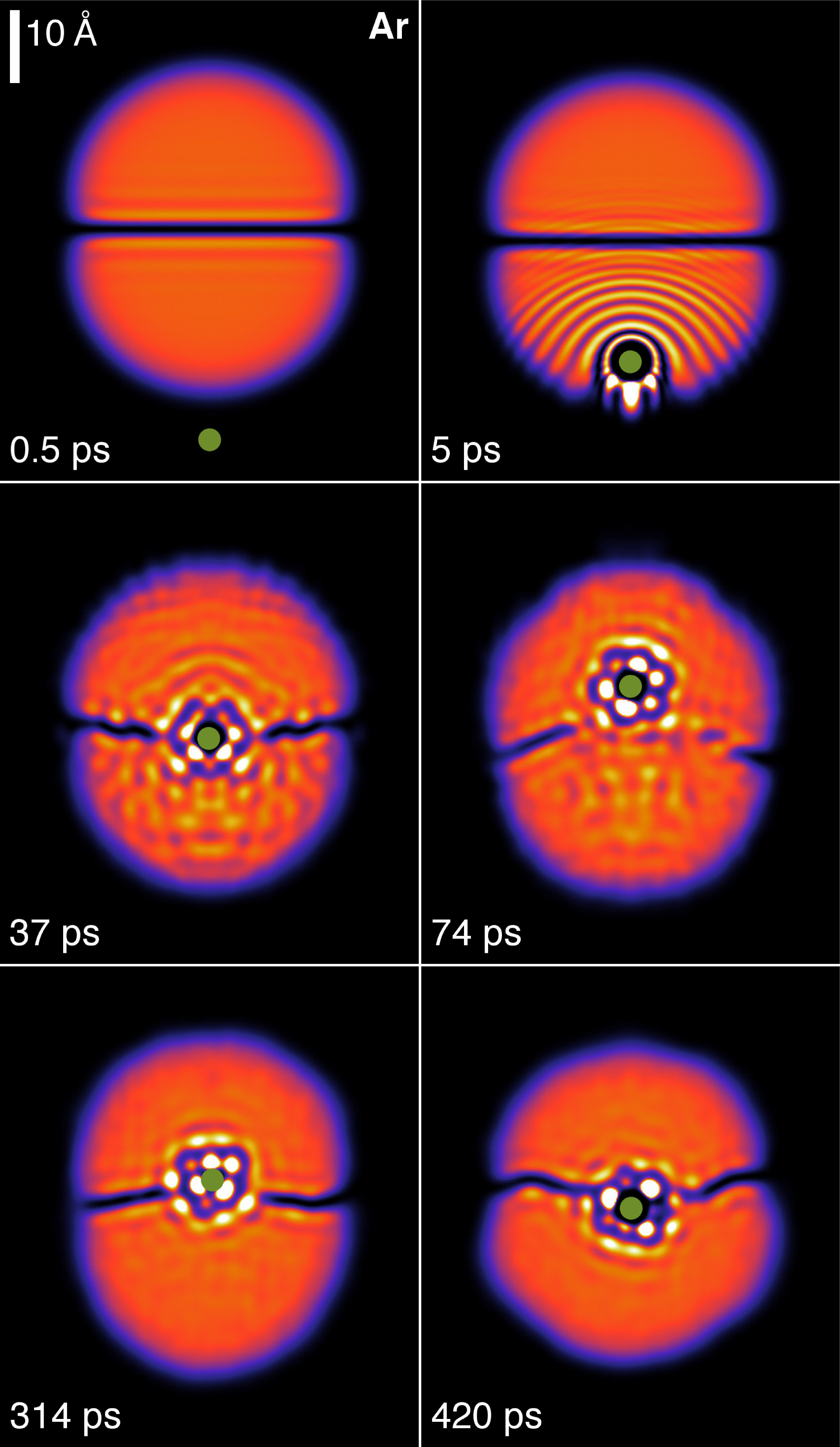
Figure 39: (a) Simulation of an Ar atom (green dot) approaching a ⁴He₁₀₀₀ droplet from below at $v_{0}=360$ m/s. The corresponding time is indicated in each frame. (b) Same as (a) but the droplet hosts a vortex line. We have included mp4 movies as Supplemental Material (on line) that show the complete simulations corresponding to this figure.

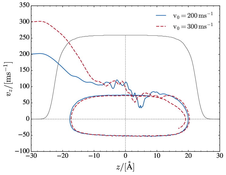
Figure 40: Phase space evolution of the Xe atom for two values of the initial velocity $v_{0}$ (200 and 300 m/s) during a head-on collision with a ⁴He₁₀₀₀ droplet. The initial droplet density profile is also shown in arbitrary density scale.

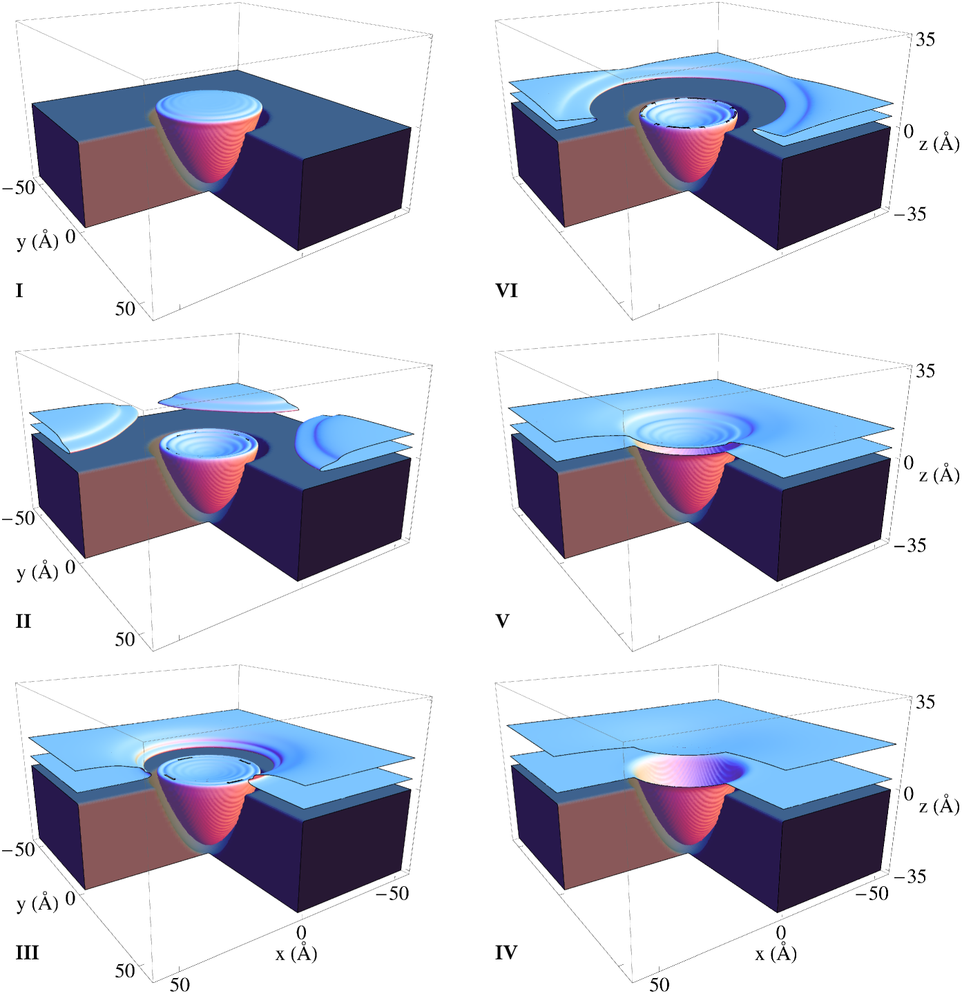
Figure 41: Liquid ⁴He on a Na patterned surface.Anc09b The panels show some illustrative equilibrium configurations for different coverages; the panels display the isodensity surfaces drawn at a value which is half the bulk liquid density at $T=0$ ($\rho_{0}=0.0218$ Å^-3). The dark area represents the Na planar surface.

V.15 Capture of impurities by ⁴He droplets

The previous sections frequently consider situations that appear after an impurity has been captured by a helium droplet or after it has been injected into liquid helium. It is well known that helium droplets are able to capture atoms and molecules, as first shown for Ne atoms.Sch90 This finding has had a tremendous impact on low temperature experiments as the technique allows to use helium droplets as an ultra-cold matrix.Toe04

The pickup process of gas phase Ar, Kr, and Xe atoms by ⁴He_N droplets ($N_{4}>10^{3}$ atoms) produced in nozzle-beam expansions was first studied by Toennies and co-workers.Lew95 These experiments characterised the deflection of a helium droplet beam by a secondary crossed beam made of rare gas atoms. This cross-beam technique was later used to characterize the helium droplet density in the beam by comparing the measured integral cross-section with the helium droplet density profiles predicted by DFT calculations.Har98 ; Har01

Theoretical work addressing the capture process is scarce. The earliest work on the scattering of ⁴He atoms by ⁴He droplets was largely inspired by the nuclear physics optical model.Eic88 More recently, scattering of helium atoms from inhomogeneous quantum liquids has also been considered.Kro07 ; Kro08

V.15.1 Pure droplets

The first TDDFT calculations modelling the capture of impurities by helium droplets were recently carried out for heliophobic (Cs)Lea14a and several heliophilic atoms (Ne, Xe and Ar).Vil16b ; Cop16 ; Cop17 The heavy impurities were treated classically whereas the lighter Ne was treated quantum mechanically; however, the collision process considered was strictly 1D (see Sec. IV.1).

Depending on the energy and the impact parameter of the impinging atom, a rich variety of dynamical phenomena may be observed.Lea14a ; Cop17 DFT calculations have shown that for a Cs atom to be trapped on the droplet surface, its excess kinetic energy must be transferred to the droplet very efficiently because the Cs-droplet binding energy is only 10.5 K. In a head-on collision with a heliophilic Xe atom, whose binding energy is 316.3 K, if the impact velocity is sufficiently high ($v_{0}>600$ m/s), the Xe atom may pass through the droplet;Cop16 otherwise it remains trapped inside. As an example, Fig. 39 shows the head-on collision of an Ar atom at $v_{0}=360$ m/s with a ⁴He₁₀₀₀ droplet.

Most of the excess kinetic energy of the impurity is deposited into the droplet, which results in the ejection of He atoms and the emission of sound and shock waves. Contrary to the naive expectation that the average energy per ejected He atom simply corresponds to its binding energy ($\sim$ 7 K), the atoms ejected at early times (prompt-emitted atoms) carry significant amounts of kinetic energy – see Table 5. Whether the impurity is heliophilic or heliophobic plays a role in the process. For example, for heliophilic Xe, 18 He atoms are ejected after 200 ps for $v_{0}$ = 200 m/s whereas only 6 He atoms are ejected in the case of heliophobic Cs during the same period of time.Lea14a

Species		$v_{0}$ (m/s)		$N_{e}$		$E_{e}$ (K)
Xe		200		18		19
		300		28		23
		400		37		30
Ar		360		16		22

Table 5: Number of ejected helium atoms ($N_{e}$) and average energy per ejected atom ($E_{e}$) for the indicated head-on collisions during the first 200 ps.Cop17

For an impurity to be captured by a helium droplet, the excess kinetic energy of the impurity must be dissipated such that it becomes less than the impurity-droplet binding energy. Fig. 40 shows the trajectory in phase space of a Xe atom captured in a ⁴He₁₀₀₀ droplet for a head-on collision at $v_{0}=200$ and 300 m/s.Cop17 It can be seen that for these collisions – corresponding to thermal velocities – the motion of the impurity inside the droplet is independent of $v_{0}$ to some extent. We attribute this to the fact that dissipation occurs mostly during the very first stages of the process.Cop16 ; Cop17

In grazing collisions not only excess energy but also angular momentum is deposited into the droplet. This allows to visualize the resulting irrotational superfluid flow inside the droplet and to calculate the capture cross-section. At low energies and small impact parameters, the impurity is captured by the droplet and may even orbit around the droplet COM.

A simple expression for the capture cross-section of classical dopants can be obtained provided that the reduced de Broglie wavelength of the impurity is much smaller than the dropletLea14a

$$\sigma(E)=\frac{\pi}{\kappa^{2}}\sum_{\ell=0}^{\ell_{cr}}(2\ell+1)=\frac{\pi}{\kappa^{2}}(\ell_{cr}+1)^{2}$$ (79)

where $E$ is the energy available in the COM frame, $\ell_{cr}$ is the critical relative angular momentum leading to impurity capture, and $\kappa=(2\mu E/\hbar^{2})^{1/2}$ with $\mu$ being the reduced mass of the system. For a given energy, $\ell_{cr}$ is determined by carrying out a series of simulations with varying impact parameters. This procedure was implemented for CsLea14a and recently also for Xe.Cop17

For a Xe atom at $v_{0}=200$ m/s, the impact parameter leading to its capture is approximately 20.5 Å, which can be compared with the sharp-density radius of the ⁴He₁₀₀₀ droplet, 22.2 Å. Hence, at thermal velocities the calculated cross-section for Xe capture is close to the geometrical cross-section of the droplet itself. The angular momentum of the impinging Xe at $v_{0}=200$ m/s with an impact parameter of 22.2 Å is 917 $\hbar$. This collision was simulated for 200 psCop17 and it was found that 15 He atoms were ejected during this time period, of which 5 remained attached to the Xe atom. After the collision, the Xe+⁴He₅ complex carries away 522 $\hbar$ angular momentum units, while some 95 $\hbar$ units are deposited into the droplet as vortex loops and capillary waves. The remaining angular momentum is taken away by the promptly emitted He atoms.

V.15.2 Droplets hosting vortices

Recently, an experimental technique for determining the size of large He droplets ($N_{4}>10^{5}$) has been introducedGom11 that is based on the attenuation of a continuous droplet beam through collisions with Ar atoms at room temperature. The pickup chamber of the droplet beam apparatus is filled with argon gas and the helium droplets are subjected to multiple isotropic collisions with Ar atoms on their way to the detection chamber; large helium droplets could also be doped by impurities using this approach. The experimental situation for large superfluid He droplets is discussed in Ref. Tan17, .

This method has been instrumental for visualizing quantised vortex arrays in large helium droplets ($10^{8}-10^{11}$ atoms) doped with Xe atoms and clusters.Gom14 ; Jon16 ; Ber17 Although experimental data for Ar was also recorded, the analysis has been limited so far to Xe because of the higher sensitivity in coherent x-ray diffractive imaging. These experiments have motivated a series of TDDFT simulations on the impurity capture process by vortex lines at impact velocities relevant to the experimental conditions.

The capture of thermal Ar and Xe atoms by a linear vortex line hosted inside a ⁴He₁₀₀₀ droplet has been recently studied by TDDFT.Cop17 The vortex line was generated by the imprinting method described in Sec. III.2 and the perpendicular impurity-vortex impact took place on the equatorial plane of the droplet at 240 (Xe) or 360 m/s (Ar). In both cases, the impurity is ‘captured’ by the vortex line in the sense that, after a few hundred ps, it orbits around the vortex line and remains at a close distance from it.Psh16 ; Cop17

The right panel of Fig. 39 shows snapshots of the collision process for Ar ($v_{0}=360$ m/s) with a ⁴He₁₀₀₀ droplet hosting a single vortex line. These data, together with those in the left panel, show the corresponding Ar atom trajectories with and without a vortex line. The first turning point of Ar in a vortex-free droplet is reached at 68 ps, and is located close to the droplet surface. The equivalent configuration in the presence of a vortex line is shown by the snapshot at 74 ps. The vortex-free configurations at 311 and 410 ps correspond to the 4^th and 5^th turning points of the Ar trajectory. Similar configurations hosting a vortex line are shown in the right panel, which demonstrates that the Ar atom trajectory becomes localised in the immediate neighborhood of the vortex line due to the impurity-vortex binding. Note that additional sources of dissipation (e.g. viscosity), which are not included in TDDFT, may only enhance this localisation process.

V.16 Liquid helium on nanostructured surfaces

As a consequence of the extremely weak He-He interaction, it is expected that liquid helium interacts strongly with almost any substrate and wet the surface such that the vapor and the substrate are not in contact. However, since the interaction of helium with alkali atoms is even weaker than the He-He interaction, they might represent a notable exception to this rule. Indeed, while liquid ³He wets any substrate, it has been shown that liquid ⁴He does not wet surfaces made of heavy alkali metals such as Cs at $T=0$.Che91 ; Tab92

The wetting properties of ⁴He on the surface of heavy alkali metals have been studied in the past by using a $T$-dependent free-energy density functional, which describes the surface properties of liquid ⁴He accurately in the $0<T<3$ K temperature range.Anc00 The resulting liquid structure on the Cs surface was elucidated, providing both the $T$-dependence of the contact angle and the wetting temperature, which are in good agreement with experiments.

The most recent research employing DFT to study the adsorption of helium samples on various substrates has been reviewed in Ref. Anc09c, . The issues addressed in this review include the deposition and spreading of helium droplets on flat alkali metal surfaces; the determination of isotherms; the construction of the phase diagram of helium on such substrates; the adsorption of helium on spherical and cylindrical surfaces; the filling of wedges and the filling/emptying transitions at $T=0$ taking place at fixed values of the wedge opening angle;Her06 the filling of infinite polygonal pores, and the adsorption on planar surfaces structured with an array of parabolic nanocavities. In particular, the prewetting line and isotherms for helium-Cs adsorbed on nano-patterned surfaces with parabolic cavities were studied by the finite temperature DFT approach.Anc00 ; Anc09b The results obtained for Cs surfaces (non-wettable) were compared with the corresponding planar Na (wettable at $T=0$) and nano-patterned Na surfaces.

To illustrate how wetting of a patterned surface proceeds, we show some configurations in Fig. 41 for the wetting sequence of a Na surface at $T=0.5$ K, from low to higher coverage. The Na surface is patterned with an array of periodically repeated parabolic cavities of nanoscopic size, and the He coverage is increased continuously. Panel I shows the low coverage phase up to the complete filling of each heliophilic parabolic cavity; in panel II, droplets grow on the flat region between the periodically repeated cavities as coverage increases; in panel III the drops on the flat region have merged together and only a ring-shaped region around the edge of the cavity remains covered by a thin helium film. Finally, complete filling of the annular region occurs (panels IV and V); at relatively higher coverages, a very thick film made of several monolayers covers the surface and grows continuously with increasing coverage (panel VI).

V.17 Soft-landing of helium droplets

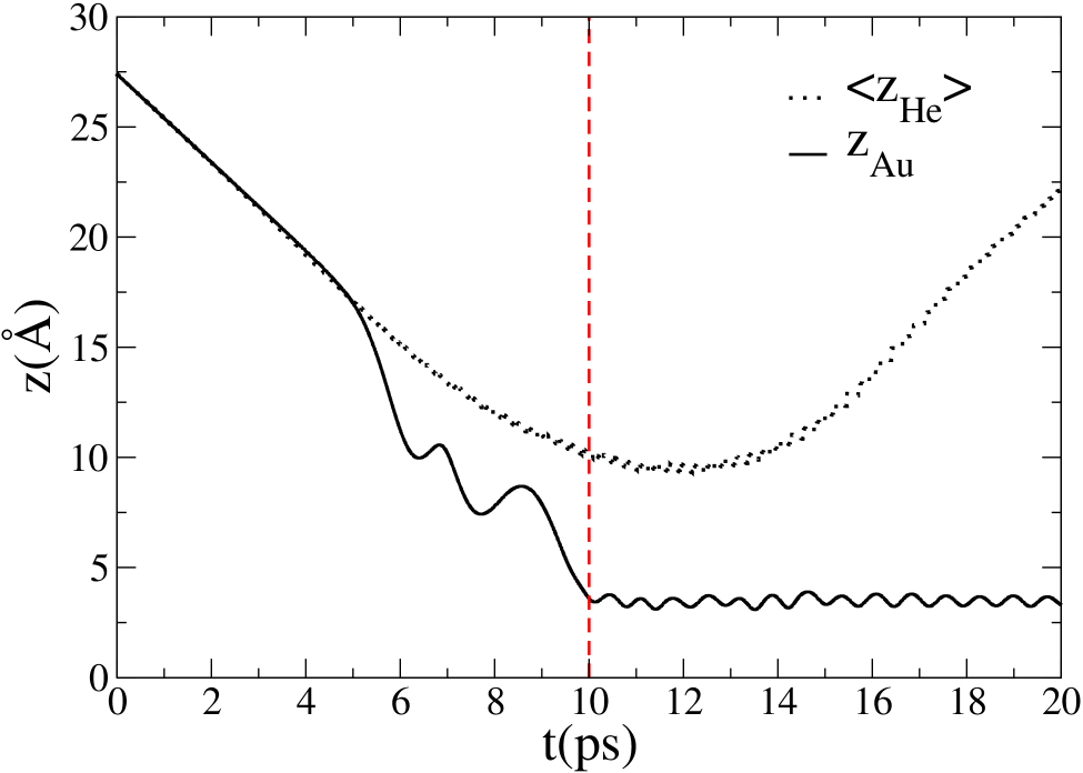
Figure 42: Au@⁴He₃₀₀ landing on rutile TiO${}_{2}(110)$-surface at 200 m/s. (a) Droplet density on a plane perpendicular to the surface at $t=10$ ps. Bright spots correspond to high helium densities and the Au atom is represented by a green dot. (b) Position of the Au atom (solid line) and the COM of the helium droplet (dotted line) with respect to the surface plane. The vertical dashed line indicates the time corresponding to the snapshot shown in (a).deL15

The time-dependent process of helium droplet landing on solid surfaces, which bears similarities with the surface wetting process discussed in the previous section, has been studied by TDDFT. In addition to contributing to the understanding of the basic physics governing such a collision event, the species formed inside the droplets can be gently deposited onto the surface (soft-landing). With the recent general interest in nano-sciences and nano-technology, this approach has received significant attention because it can potentially be used to extract the nanostructures formed inside helium droplets for practical applications.Moz07 ; Log11d For example, metallic nanoclusters and nanowires, which are predicted to be excellent catalysts due to their large surface area, could be produced by using this technique. For a review on soft-landing, see Ref. Joh11, .

Soft-landing of metal (e.g. Ag) doped large helium droplets has also been instrumental for the discovery of vortex lines inside the droplets.Gom12 ; Lat14 ; Tha14 The experiments revealed the presence of linear structures on the deposition surface along which a series of nanoparticles were distributed. The observed linear geometries have been suggested to arise either from vortex mediated nanowire assembly (and subsequent decomposition) or from direct trapping of multiple metal nanoparticles on a vortex line. Both mechanisms require the presence of quantized vortices inside the droplets.

The first TDDFT studies for the softlanding of pure helium droplets on surfaces with potential technological interest have been carried recently.Agu12 ; deL14 The model system considered consisted of a ⁴He₃₀₀ droplet traveling at 200 m/s towards a TiO₂ (110)-surface. To identify the possible quantum effects, both classical molecular dynamics and TDDFT simulations were carried out. In contrast to the classical results, which show the helium droplet splashing off the surface on impact, the TDDFT evolution leads to the spreading of the liquid on the surface. This thin film formation is a process similar to the surface wetting described in the previous section. In addition to TiO₂, a graphite sheet was also considered as a target.deL14 Despite the omission of thermal effects and the small droplet size considered, these studies have provided a solid starting point for simulating helium droplet mediated deposition of metallic clusters on substrates.

Deposition of an Au atom embedded inside a ⁴He₃₀₀ droplet on a TiO₂ (110)-surface was addressed in Ref. deL15, . This was the first theoretical study that considered the experimentally studied landing process as described e.g. in Refs. Moz07, ; Log11d, ; Vol13, . The outcome of the simulation for an Au@⁴He₃₀₀ complex at 200 m/s, with COM initially located at 27.4 Å from the surface, is shown in Fig. 42. As shown in the figure, the Au atom initially follows the droplet, then begins to oscillate back and forth inside it, and finally becomes trapped inside the Au-TiO₂ surface potential minimum. After ca. 10 ps, the atom keeps oscillating about the potential energy minimum until the end of the simulation (zero average acceleration). The spreading of the droplet on the surface was observed, but to a lesser degree than for the pure helium droplet.Agu12 By comparing the results from TDDFT and classical calculations, it was concluded that the proper description of this ⁴He droplet-assisted process must be carried out using quantum mechanical simulations.

VI Summary and outlook

The density functional approach offers a unique method to study both static and dynamic response of superfluid helium. In addition to atomic and molecular impurities, it can also be applied in its present form to model the interaction of nanometer-scale objects with the liquid. From the computational resource perspective, the method is easily applied to systems up to 100 nm in size in 3D, the main limitations being both computer time and memory requirements. The formulation allows for the description of both helium droplets and bulk liquid through suitable boundary conditions. With the recent improvements to the OT-DFT functional, strongly inhomogeneous snowball systems can now be modelled. Unlike QMC-based methods, DFT can yield real time quantum dynamics. The examples summarised in this review provide extensive evidence that the TDDFT approach is capable of reproducing the results from a wide range of time-resolved experiments, especially in superfluid helium droplets. It is the only method that allows this close interplay between theory and experiment in this field.

Despite the enormous success of OT-DFT, and DFT in general, there is still room for improvement in both accuracy and functionality. For example, just like any other DFT-based method, it is not straightforward to couple DFT to any degrees of freedom that follow traditional quantum mechanics. The often employed coupled quantum and OT-DFT equations presented in this review all either ignore the quantum correlations between the two subsystems or incorporate them in a phenomenological way into the interaction potential. In many systems, such as the electron bubble, this correlation may not be significant due to the large mass difference between the electron and helium. But it will arise, for example, in the treatment of molecular rotation in superfluid helium. Up to now the latter problem has only been addressed in terms of classical rotation and the associated moment of inertia, which is the likely origin of the remaining discrepancy between the OT-DFT calculations and experimental results (Sec. V.11). A similar issue should arise in the treatment of molecular vibrations of impurities solvated in superfluid helium.

While PIMC calculations can elegantly model superfluid helium at finite temperatures, OT-DFT in its basic formulation is restricted to 0 K. The static liquid response up to 3 K temperature has been introduced into OT-DFT, but it is still missing dynamic contributions such as the viscous response. The viscous response can be included from continuum fluid mechanics (Navier-Stokes) into OT-DFT, but it is not a priori clear how it should behave at the typically observed rather wide gas-liquid interfaces around solvated impurities. In general, one possible strategy may be to follow the very successful Landau’s two-fluid model and treat the superfluid and normal fractions in DFT separately.

Many elegant experiments have been carried out in bulk superfluid helium over the years, which would require at least a mesoscopic-size description of the system. Therefore, they are currently not accessible to the OT-DFT approach due to the limitations in current computational resources. In order to employ the DFT approach for such systems, new strategies are needed to reduce especially the memory requirements of the calculations. An obvious approach is to use any symmetry present in the system and formulate the problem in 1D or 2D rather than the full 3D. However, often such symmetry is not present and furthermore, the numerical implementation of OT-DFT in reduced dimensions is sometimes far from trivial.

If a distant part of the system can be treated with a limited accuracy, multi-scale-type models could be developed to expand the spatial domain considered. Another option would be to vary the resolution of the spatial grid, which allows allocating more points to the regions of interest. However, all current numerical implementations of OT-DFT are restricted to uniform grids because they employ the finite difference approximation and the FFT algorithm for evaluating the non-linear potential. While the well-known finite element method could replace the finite difference approach, the heavily used FFT would still not be applicable for non-uniform grids.

Notwithstanding the need for improvements, the applications of the current OT-DFT approach, especially in its time-dependent version, are noteworthy. Among the projects that are being conducted during the completion of this review, let us mention e.g. the desorption of intrinsic and extrinsic impurities from helium droplets; the description of soft-landing processes under conditions closer to the experimental situation; the multiple capture of impurities by droplets hosting vortex arrays, and the propagation of shock waves and solitons, and gas bubble dynamics and vortex nucleation in liquid helium.

Finally, let us indicate that the CSU at Northridge and Barcelona-Toulouse helium-DFT codes are available at the following repositories:

$\bullet$ CSU at Northridge He-DFT code:

https://sourceforge.net/projects/libgrid/

https://sourceforge.net/projects/libdft/

$\bullet$ BCN-TLS DFT He-code:

https://github.com/bcntls2016/4hedft

https://github.com/bcntls2016/4hedft-vortex

https://github.com/bcntls2016/4hetddft-isotropic

https://github.com/bcntls2016/4hetddft-anisotropic

- (1) D. R. Tilley and J. Tilley, Superfluidity and superconductivity (John Wiley & Sons, New York, 1974).
- (2) A. F. Borghesani, Ions and electrons in liquid helium (Oxford Science Publications, New York, 2007).
- (3) M. Hartmann, R. E. Miller, J. P. Toennies, and A. F. Vilesov, Phys. Rev. Lett. 75, 1566 (1995).
- (4) M. Hartmann, F. Mielke, J. P. Toennies, A. F. Vilesov, and G. Benedek, Phys. Rev. Lett. 76, 4560 (1996).
- (5) K. K. Lehmann and G. Scoles, Science 279, 2065 (1998).
- (6) J. P. Toennies and A. F. Vilesov, Angew. Chem. Phys. 43, 2622 (2004).
- (7) M. Barranco, R. Guardiola, S. Hernández, R. Mayol, J. Navarro, and M. Pi, J. Low Temp. Phys. 142, 1 (2006).
- (8) K. Szalewicz, Int. Rev. Phys. Chem. 27, 273 (2006).
- (9) F. Stienkemeier and K. K. Lehmann, J. Phys. B 39, R127 (2006).
- (10) M. Y. Choi, G. E. Douberly, T. M. Falconer, W. K. Lewis, C. M. Lindsay, J. M. Merritt, P. L. Stiles, and R. E. Miller, Int. Rev. Phys. Chem. 25, 15 (2006).
- (11) J. Tiggesbäumker and F. Stienkemeier, Phys. Chem. Chem. Phys. 9, 4748 (2007).
- (12) A. Slenczka and J. P. Toennies, in Low Temperatures and Cold Molecules, edited by W. M. Smith (World Sci., Singapore, 2008), p. 345.
- (13) C. Callegari and W. E. Ernst, in Handbook of High Resolution Spectroscopy, Vol. 3 (Whiley, New York, 2011), p. 1551.
- (14) S. Yang and A. M. Ellis, Chem. Soc. Rev 42, 472 (2013).
- (15) M. Mudrich and F. Stienkemeier, Int. Rev. Phys. Chem. 33, 301 (2014).
- (16) J. P. Toennies, The Chemical physics of Atomic and Molecular Clusters, Course CVII, in Proceedings of the International School of Physics “Enrico Fermi” 1988 (North Holland, Amsterdam, 1990), p. 597.
- (17) K. B. Whaley, Int. Rev. Phys. Chem. 13, 41 (1994).
- (18) K. B. Whaley, Advances in Molecular Vibrations and Collision Dynamics 3, 397 (1998).
- (19) J. P. Toennies and A. F. Vilesov, Ann. Rev. Phys. Chem. 49, 1 (1998).
- (20) J. A. Northby, J. Chem. Phys. 115, 10065 (2001), Special Topic issue on Helium nanodroplets.
- (21) E. Krotscheck and J. Navarro, editors, Microscopic approaches to quantum liquids in confined geometries, Series on Advances in Quantum Many-Body Theory, Vol. 4 (World Scientific, Singapore, 2002).
- (22) M. P. de Lara-Castells, G. Delgado-Barrio, P. Villarreal, and A. O. Mitrushchenkov, J. Chem. Phys. 125, 221101 (2006).
- (23) M. P. de Lara-Castells, N. F. Aguirre, P. Villarreal, G. Delgado-Barrio, and A. O. Mitrushchenkov, J. Chem. Phys. 132, 194313 (2010).
- (24) N. F. Aguirre, P. Villarreal, G. Delgado-Barrio, A. O. Mitrushchenkov, and M. P. de Lara-Castells, Phys. Chem. Chem. Phys. 15, 10126 (2013).
- (25) S. Stringari and J. Treiner, Phys. Rev. B 36, 8369 (1987).
- (26) S. Stringari and J. Treiner, J. Chem. Phys. 87, 5021 (1987).
- (27) F. Dalfovo, A. Lastri, L. Pricaupenko, S. Stringari, and J. Treiner, Phys. Rev. B 52, 1193 (1995).
- (28) M. P. Ziemkiewicz, D. M. Neumark, and O. Gessner, Int. Rev. Phys. Chem. 34, 239 (2015).
- (29) L. F. Gomez, K. R. Ferguson, J. P. Cryan, C. Bacellar, R. M. P. Tanyag, C. Jones, S. Schorb, D. Anielski, A. Belkacem, C. Bernando, R. Boll, J. Bozek, et al., Science 345, 906 (2014).
- (30) N. B. Brauer, S. Smolarek, E. Loginov, D. Mateo, A. Hernando, M. Pi, M. Barranco, W. J. Buma, and M. Drabbels, Phys. Rev. Lett. 111, 153002 (2013).
- (31) J. von Vangerow, F. Coppens, A. Leal, M. Pi, M. Barranco, N. Halberstadt, F. Stienkemeier, and M. Mudrich, J. Phys. Chem. Lett. 8, 307 (2017).
- (32) A. Leal, D. Mateo, A. Hernando, M. Pi, M. Barranco, A. Ponti, F. Cargnoni, and M. Drabbels, Phys. Rev. B 90, 224518 (2014).
- (33) S. L. Fiedel, D. Mateo, T. Aleksanyan, and J. Eloranta, Phys. Rev. B 86, 144522 (2012).
- (34) M. Barranco, F. Coppens, N. Halberstadt, A. Hernando, A. Leal, D. Mateo, R. Mayol, and M. Pi, Zero temperature DFT and TDDFT for 4He: A short guide for practitioners (2017), https://github.com/bcntls2016/DFT-Guide/blob/master/dft-guide.pdf.
- (35) D. Mateo, M. Barranco, and J. Navarro, Phys. Rev. B 82, 134529 (2010).
- (36) R. J. Donnelly, J. A. Donnelly, and R. N. Hills, J. Low Temp. Phys. 44, 471 (1981).
- (37) P. Hohenberg and W. Kohn, Phys. Rev. 136, B864 (1964).
- (38) W. Kohn and L. J. Sham, Phys. Rev. 140, A1133 (1965).
- (39) E. Runge and E. K. U. Gross, Phys. Rev. Lett. 52, 997 (1984).
- (40) E. Madelung, Z. Phys. 40, 322 (1927).
- (41) F. Ancilotto, M. Barranco, and M. Pi, Phys. Rev. B 82, 014517 (2010).
- (42) E. Popov and J. Eloranta, J. Chem. Phys. 142, 204704 (2015).
- (43) D. Mateo, J. Eloranta, and G. A. Williams, J. Chem. Phys. 142, 064510 (2015).
- (44) D. Mateo, A. Hernando, M. Barranco, E. Loginov, M. Drabbels, and M. Pi, Phys. Chem. Chem. Phys. 15, 18388 (2013).
- (45) N. G. Berloff and P. H. Roberts, J. Phys. A 34, 81 (2001).
- (46) D. Mateo, D. Jin, M. Barranco, and M. Pi, J. Chem. Phys. 134, 044507 (2011).
- (47) D. Jin and H. J. Maris, J. Low Temp. Phys. 158, 317 (2010).
- (48) D. Jin and W. Guo, Phys. Rev. B 82, 094524 (2010).
- (49) D. Jin, W. Guo, W. Wei, and H. J. Maris, J. Low Temp. Phys. 158, 307 (2010).
- (50) I. A. Pshenichnyuk and N. G. Berloff, Phys. Rev. B 94, 184505 (2016).
- (51) F. Ancilotto, F. Faccin, and F. Toigo, Phys. Rev. B 62, 17035 (2000).
- (52) T. Biben and D. Frenkel, J. Phys. Cond. Matt. 14, 9077 (2002).
- (53) D. Jin and W. Guo, J. Chem. Phys. 136, 244510 (2012).
- (54) M. Barranco, M. Pi, S. M. Gatica, E. S. Hernández, and J. Navarro, Phys. Rev. B 56, 8997 (1997).
- (55) A. Leal, D. Mateo, M. Pi, M. Barranco, and J. Navarro, J. Chem. Phys. 139, 174308 (2013).
- (56) A. Hernando, R. Mayol, M. Pi, M. Barranco, F. Ancilotto, O. Bünermann, and F. Stienkemeier, J. Phys. Chem. A 111, 7303 (2007).
- (57) E. S. Hernández and J. Navarro, in Microscopic approaches to quantum liquids in confined geometries, edited by E. Krotscheck and J. Navarro (World Sci, Singapore, 2002), p. 261.
- (58) M. Abad, M. Guilleumas, R. Mayol, M. Pi, and D. M. Jezek, Phys. Rev. A 81, 043619 (2010).
- (59) F. Ancilotto, M. Barranco, J. Navarro, and M. Pi, J. Low Temp. Phys. 185, 26 (2016).
- (60) F. Ancilotto, M. Barranco, F. Caupin, R. Mayol, and M. Pi, Phys. Rev. B 72, 214522 (2005).
- (61) F. Caupin, F. Ancilotto, M. Barranco, R. Mayol, and M. Pi, J. Low Temp. Phys. 148, 731 (2007).
- (62) F. Ancilotto, M. Pi, R. Mayol, M. Barranco, and K. K. Lehmann, J. Phys. Chem. A 111, 12695 (2007).
- (63) R. P. Feynman and M. Cohen, Phys. Rev. 102, 1189 (1956).
- (64) M. R. Gibbs, K. H. Andersen, W. G. Stirling, and H. Schober, J. Phys.: Condens. Matter 11, 603 (1999).
- (65) D. J. Thouless, Ann. Phys. (N.Y.) 52, 403 (1969).
- (66) L. Giacomazzi, F. Toigo, and F. Ancilotto, Phys. Rev. B 67, 104501 (2003).
- (67) L. Lehtovaara, T. Kiljunen, and J. Eloranta, J. Comput. Phys. 194, 78 (2004).
- (68) L. Lehtovaara, J. Toivanen, and J. Eloranta, J. Comput. Phys. 221, 148 (2007).
- (69) M. Pi, R. Mayol, A. Hernando, M. Barranco, and F. Ancilotto, J. Chem. Phys. 126, 244502 (2007).
- (70) M. Frigo and S. G. Johnson, Proc. IEEE 93, 216 (2005).
- (71) F. Ancilotto, M. Pi, and M. Barranco, Phys. Rev. B 91, 100503(R) (2015).
- (72) F. Dalfovo, R. Mayol, M. Pi, and M. Barranco, Phys. Rev. Lett 85, 1028 (2000).
- (73) F. Ancilotto, M. Pi, and M. Barranco, Phys. Rev. B 90, 174512 (2014).
- (74) R. J. Donnelly, Quantized vortices in helium II, Cambridge Studies in Low Temperature Physics, Vol. 3 (Cambridge University Press, Cambridge, U.K., 1991).
- (75) F. Dalfovo and S. Stringari, Phys. Rev. A 53, 2477 (1996).
- (76) J. von Vangerow, A. Stieg, F. Stienkemeier, M. Mudrich, A. Leal, D. Mateo, A. Hernando, M. Barranco, and M. Pi, J. Phys. Chem. A 118, 6604 (2014).
- (77) D. Mateo, A. Leal, A. Hernando, M. Barranco, M. Pi, F. Cargnoni, M. Mella, X. Zhang, and M. Drabbels, J. Chem. Phys. 140, 131101 (2014).
- (78) A. I. Krylov, Annu. Rev. Phys. Chem. 59, 433 (2008).
- (79) R. E. Wyatt, Quantum Dynamics with Trajectories (Springer, New York, 2005).
- (80) A. Hernando, M. Barranco, M. Pi, E. Loginov, M. Langlet, and M. Drabbels, Phys. Chem. Chem. Phys. 14, 3996 (2012).
- (81) F. O. Ellison, J. Am. Chem. Soc. 85, 3540 (1963).
- (82) A. Hernando, M. Barranco, R. Mayol, M. Pi, and M. Krośnicki, Phys. Rev. B 77, 024513 (2008).
- (83) J. Eloranta, J. Ahokas, and H. Kunttu, J. Chem. Phys. 114, 7144 (2001).
- (84) Z. J. Jakubek, Q. Hui, and M. Takami, Phys. Rev. Lett. 79, 629 (1997).
- (85) A. Nakayama and K. Yamashita, J. Chem. Phys. 114, 780 (2001).
- (86) A. Leal, X. Zhang, M. Barranco, F. Cargnoni, A. Hernando, D. Mateo, M. Mella, M. Drabbels, and M. Pi, J. Chem. Phys. 144, 094302 (2016).
- (87) M. Mella and F. Cargnoni, J. Phys. Chem. A 118, 6473 (2014).
- (88) A. Ralston and H. S. Wilf, Mathematical methods for digital computers (John Wiley and Sons, New York, 1960).
- (89) W. H. Press, S. A. Teukolsky, W. T. Vetterling, and B. P. Flannery, Numerical Recipes (Cambridge University Press, Cambridge, 1992).
- (90) D. Nettels, A. Hofer, P. Moroshkin, R. Müller-Siebert, S. Ulzega, and A. Weis, Phys. Rev. Lett. 94, 063001 (2005).
- (91) X. Buelna, A. Freund, D. Gonzalez, E. Popov, and J. Eloranta, J. Phys. Chem. B 120, 11010 (2016).
- (92) M. Barranco, J. Eloranta, A. Hernando, and M. Pi, unpublished (2016) .
- (93) S. H. Patil, J. Chem. Phys. 94, 8089 (1991).
- (94) J. Pascale, Phys. Rev. A 28, 632 (1983).
- (95) F. Stienkemeier, F. Meier, and H. O. Lutz, Eur. Phys. J. D 9, 313 (1999).
- (96) D. Mateo, A. Hernando, M. Barranco, R. Mayol, and M. Pi, Phys. Rev. B 83, 174505 (2011).
- (97) A. Hernando, M. Barranco, R. Mayol, M. Pi, F. Ancilotto, O. Bünermann, and F. Stienkemeier, J. Low Temp. Phys. 158, 105 (2010).
- (98) D. Tannor, Introduction to Quantum mechanics: A Time-Dependent Perspective (University Science Books, Sausalito, California (USA), 2007).
- (99) A. Hernando, R. Mayol, M. Pi, M. Barranco, I. S. K. Kerkines, and A. Mavridis, Int. J. of Quantum Chem. 111, 400 (2011).
- (100) J. Eloranta, H. Y. Seferyan, and V. A. Apkarian, Chem. Phys. Lett. 396, 155 (2004).
- (101) F. Ancilotto, P. B. Lerner, and M. W. Cole, J. Low Temp. Phys. 101, 1123 (1995).
- (102) F. Stienkemeier, J. Higgins, C. Callegari, S. I. Kanorsky, W. E. Ernst, and G. Scoles, Z. Phys. D 38, 253 (1996).
- (103) O. Bünermann, G. Droppelmann, A. Hernando, R. Mayol, and F. Stienkemeier, J. Phys. Chem. A 111, 12684 (2007).
- (104) F. Lackner, J. Poms, G. Krois, J. V. Pototschnig, and W. E. Ernst, J. Phys. Chem. A 117, 11866 (2013).
- (105) C. Callegari and F. Ancilotto, J. Phys. Chem. A 115, 6789 (2011).
- (106) A. Pifrader, O. Allard, G. Auböck, C. Callegari, W. E. Ernst, R. Hubert, and F. Ancilotto, J. Chem. Phys. 133, 164502 (2010).
- (107) E. Loginov, C. Callegari, F. Ancilotto, and M. Drabbels, J. Phys. Chem. A 115, 6779 (2011).
- (108) L. Fechner, B. Grüner, A. Sieg, C. Callegari, F. Ancilotto, F. Stienkemeier, and M. Mudrich, Phys. Chem. Chem. Phys. 14, 3843 (2012).
- (109) A. Hernando, J. A. Beswick, and N. Halberstadt, J. Chem. Phys. 139, 221102 (2013).
- (110) E. Loginov, A. Hernando, J. A. Beswick, N. Halberstadt, and M. Drabbels, J. Phys. Chem. A 119, 6033 (2015).
- (111) B. Gervais, D. Zanuttini, and J. Douady, J. Chem. Phys. 144, 194307 (2016).
- (112) J. D. Close, F. Federman, K. Hoffmann, and N. Quass, J. Low Temp. Phys. 111, 661 (1998).
- (113) D. Mateo, A. Hernando, M. Barranco, and M. Pi, J. Low Temp. Phys. 158, 397 (2010).
- (114) F. Stienkemeier, F. Meier, and H. O. Lutz, J. Chem. Phys. 107, 10816 (1997).
- (115) F. Ancilotto, M. Barranco, and M. Pi, Phys. Rev. Lett. 91, 105302 (2003).
- (116) C. F. Jones, C. Bernando, R. M. P. Tanyag, C. Bacellar, K. R. Ferguson, L. F. Gomez, D. Anielski, A. Belkacem, R. Boll, J. Bozek, S. Carron, J. Cryan, et al., Phys. Rev. B 93, 180510(R) (2016).
- (117) C. Bernando, R. Mayro, P. Tanyag, C. Jones, C. Bacellar, M. Bucher, K. R. Ferguson, D. Rupp, M. P. Ziemkiewicz, L. F. Gomez, A. S. Chatterley, T. Gorkhover, et al., Phys. Rev. B 95, 064510 (2017).
- (118) Y. Moriwaki and N. Morita, Eur. Phys. J. D 33, 323 (2005).
- (119) A. Hernando, M. Barranco, R. Mayol, M. Pi, and F. Ancilotto, Phys. Rev. B 78, 184515 (2008).
- (120) M. Mella, G. Calderoni, and F. Cargnoni, J. Chem. Phys. 123, 054328 (2005).
- (121) J. Navarro, D. Mateo, M. Barranco, and A. Sarsa, J. Chem. Phys. 136, 054301 (2012).
- (122) E. Krotscheck and R. E. Zillich, J. Chem. Phys. 145, 244317 (2016).
- (123) J. Reho, U. Merker, M. R. Radcliff, K. K. Lehmann, and G. Scoles, J. Chem. Phys. 112, 8409 (2000).
- (124) A. Przystawik, S. Göde, T. Döppner, J. Tiggesbäumker, and K-H. Meiwes-Broer, Phys. Rev. A 78, 021202(R) (2008).
- (125) Y. Ren and V. V. Kresin, Phys. Rev. A 76, 043204 (2007).
- (126) M. Lewerenz, B. Schilling, and J. P. Toennies, J. Chem. Phys. 102, 8191 (1995).
- (127) E. B. Gordon, J. Low Temp. Phys. 30, 756 (2004).
- (128) J. Eloranta, Phys. Rev. B 77, 134301 (2008).
- (129) A. W. Hauser, A. Volk, P. Thaler, and W. E. Ernst, Phys. Chem. Chem. Phys. 17, 10805 (2015).
- (130) J. Eloranta, Low Temp. Phys. 37, 384 (2011).
- (131) S.Göde, R. Irsing, J. Tiggesbäumker, and K-H. Meiwes-Broer, New J. Phys. 15, 015026 (2013).
- (132) A. Hernando, F. Ancilotto, M. Barranco, R. Mayol, and M. Pi, J. of Physics: Conf. Ser. 150, 032003 (2009).
- (133) E. Loginov, L. F. Gomez, N. Chiang, A. Halder, N. Guggemos, V. V. Kresin, and A. F. Vilesov, Phys. Rev. Lett. 106, 233401 (2011).
- (134) E. Lugovoj, J. P. Toennies, and A. F. Vilesov, J. Chem. Phys. 112, 8217 (2000).
- (135) G. E. Douberly, P. L. Stiles, R. E. Miller, R. Schmied, and K. K. Lehmann, J. Phys. Chem. A 114, 3391 (2010).
- (136) A. Masson, M. Briant, A. Hernando, N. Halberstadt, J.-M. Mestdagh, and M.-A. Gaveau, J. Chem. Phys. 137, 184310 (2012).
- (137) A. Hernando, A. Masson, M. Briant, J.-M. Mestdagh, M.-A. Gaveau, and N. Halberstadt, J. Chem. Phys. 137, 184311 (2012).
- (138) J. Poms, A. W. Hauser, and W. E. Ernst, Phys. Chem. Chem. Phys. 14, 15165 (2012).
- (139) M. Renzler, M. Daxner, L. Kranabetter, A. Kaiser, A. W. Hauser, W. E. Ernst, A. Lindinger, and R. E. Zillich, J. Chem. Phys. 145, 181101 (2016).
- (140) J. Höller, E. Krotscheck, and R. E. Zillich, Eur. Phys. J. D 69, 198 (2015).
- (141) C. Stark and V. V. Kresin, Phys. Rev. B 81, 085401 (2010).
- (142) L. An der Lan, P. Bartl, C. Leidlmair, H. Schöbel, R. Jochum, S. Denifl, T. D. Märk, A. M. Ellis, and P. Scheier, J. Chem. Phys. 135, 044309 (2011).
- (143) F. Calvo, Phys. Rev. B 95, 035429 (2017).
- (144) J. Höller, E. Krotscheck, and R. E. Zillich, Eur. Phys. J. D 68, 372 (2014).
- (145) Y. Kwon and H. Shin, Phys. Rev. B 82, 172506 (2010).
- (146) H. Shin and Y. Kwon, J. Chem. Phys. 136, 064514 (2012).
- (147) D. Bonhommeau, P. T. Lake Jr., C. L. Quiniou, M. Lewerenz, and N. Halberstadt, J. Chem. Phys. 126, 051104 (2007).
- (148) D. Bonhommeau, M. Lewerenz, and N. Halberstadt, J. Chem. Phys. 128, 054302 (2008).
- (149) V. Mozhayskiy, M. N. Slipchenko, V. K. Adamchuk, and A. F. Vilesov, J. Chem. Phys. 127, 094701 (2007).
- (150) E. Loginov, L. F. Gomez, and A. F. Vilesov, Phys. Chem. A 117, 11771 (2013).
- (151) A. W. Hauser and M. P. de Lara-Castells, J. Phys. Chem. Lett. 7, 4929 (2016).
- (152) A. W. Hauser, A. O. Mitrushchenkov, and M. P. de Lara-Castells, J. Phys. Chem. C 121, 3807 (2017).
- (153) B. E. Clements, E. Krotscheck, and H. J. Lauter, Phys. Rev. Lett. 70, 1287 (1993).
- (154) E. S. Hernández, J. Low Temp. Phys. 162, 583 (2011).
- (155) S. Grebenev, J. P. Toennies, and A. F. Vilesov, Science 279, 2083 (1998).
- (156) O. Bünermann, M. Dvorak, F. Stienkemeier, A. Hernando, R. Mayol, M. Pi, M. Barranco, and F. Ancilotto, Phys. Rev. B 79, 214511 (2009).
- (157) R. Guardiola, J. Navarro, D. Mateo, and M. Barranco, J. Chem. Phys. 131, 174110 (2009).
- (158) L. S. Cederbaum, J. Zobeley, and F. Tarantelli, Phys. Rev. Lett. 79, 4778 (1997).
- (159) N. V. Kryzhevoi, D. Mateo, M. Pi, M. Barranco, and L. S. Cederbaum, Phys. Chem. Chem. Phys. 15, 18167 (2013).
- (160) N. V. Kryzhevoi, V. Averbukh, and L. S. Cederbaum, Phys. Rev. B 76, 094513 (2007).
- (161) M. Shcherbinin, A. C. LaForge, V. Sharma, M. Devetta, R. Richter, R. Moshammer, T. Pfeifer, and M. Mudrich, submitted to Phys. Rev. Lett. (2017).
- (162) M. Guilleumas, F. Garcias, M. Barranco, M. Pi, and E. Suraud, Z. Phys. D 26, 385 (1993).
- (163) D. Mateo, M. Barranco, R. Mayol, and M. Pi, Eur. Phys. J. D 52, 63 (2009).
- (164) D. Mateo, M. Barranco, R. Mayol, J. Navarro, and M. Pi, J. of Physics: Conf. Ser. 150, 032051 (2009).
- (165) B. G. Sartakov, J. P. Toennies, and A. F. Vilesov, J. Chem. Phys. 136, 134316 (2012).
- (166) D. Mateo, M. Pi, J. Navarro, and J. P. Toennies, J. Chem. Phys. 138, 044321 (2013).
- (167) N. Pörtner, J. P. Toennies, A. F. Vilesov, G. Benedek, and W. Hizhnyakov, Europhys. Lett. 88, 26007 (2009).
- (168) G. Benedek and V. Hizhnyakov, Chem. Phys. Lett. 548, 17 (2012).
- (169) J. Barragán, D. Mateo, M. Pi, F. Salvat, M. Barranco, and H. J. Maris, J. Low Temp. Phys. 171, 171 (2013).
- (170) M. Barranco, M. Guilleumas, M. Pi, and D. M. Jezek, in Microscopic approaches to quantum liquids in confined geometries, edited by E. Krotscheck and J. Navarro (World Sci, Singapore, 2002), p. 319.
- (171) S. Balibar, J. Low Temp. Phys. 129, 363 (2002).
- (172) H. J. Maris, J. Phys. Soc. Jpn. 77, 111008 (2008).
- (173) B. Tabbert, H. Günther, and G. zu Putlitz, J. Low Tem. Phys. 109, 653 (1997).
- (174) K. Coutinho, S. Canuto, P. K. Mukherjee, and B. Fricke, in Advances in the Theory of Atomic and Molecular Systems: Dynamics, Spectroscopy, Clusters, and Nanostructures, edited by P. Piecuch, J. Maruani, G. Delgado-Barrio, and S. Wilson (Springer Netherlands, Dordrecht, 2009), p. 183.
- (175) H. J. Maris, J. Low Temp. Phys. 173, 78 (2000).
- (176) W. Wei, Z. Xie, L. N. Cooper, G. M. Seidel, and H. J. Maris, J. Low Temp. Phys. 178, 78 (2015).
- (177) J. Tempere, I. F. Silvera, and J. T. Devreese, Sur. Sci. Rep 62, 159 (2007).
- (178) W. Guo, D. Jin, and H. J. Maris, Phys. Rev. B 78, 014511 (2008).
- (179) J. Fang, J. Tempere, and I. F. Silvera, J. Low Temp. Phys. 187, 54 (2017).
- (180) L. Lehtovaara and J. Eloranta, J. Low Temp. Phys. 148, 43 (2007).
- (181) J. Eloranta and V. A. Apkarian, J. Chem. Phys. 117, 10139 (2002).
- (182) V. Grau, M. Barranco, R. Mayol, and M. Pi, Phys. Rev. B 73, 064502 (2006).
- (183) C. C. Grimes and G. Adams, Phys. Rev. B 45, 2305 (1992).
- (184) J. Classen, C.-K. Su, M. Mohazzab, and H. J. Maris, Phys. Rev. B 57, 3000 (1998).
- (185) M. Pi, M. Barranco, R. Mayol, and V. Grau, J. Low Temp. Phys. 139, 397 (2005).
- (186) D. Mateo, M. Pi, and M. Barranco, Phys. Rev. B 81, 174510 (2010).
- (187) D. Konstantinov and H. J. Maris, Phys. Rev. Lett. 90, 025302 (2003).
- (188) H. J. Maris, A. Ghosh, D. Konstantinov, and M. Hirsch, J. Low Temp. Phys. 134, 227 (2004).
- (189) F. Ancilotto, F. Dalfovo, L. P. Pitaevskii, and F. Toigo, Phys. Rev. B 71, 104530 (2005).
- (190) G. G. Nancolas, T. Ellis, P. McClintock, and R. M. Bowley, Nature 316, 797 (1985).
- (191) S. Paolini, F. Ancilotto, and F. Toigo, J. Chem. Phys. 126, 124317 (2007).
- (192) P. Claas, S. O. Mende, and F. Stienkemeier, Rev. Sci. Instrum. 74, 4071 (2003).
- (193) A. Braun and M. Drabbels, Phys. Rev. Lett. 93, 253401 (2004).
- (194) X. Zhang and M. Drabbels, J. Chem. Phys. 137, 051102 (2012).
- (195) D. E. Galli, D. M. Ceperley, and L. Reatto, J. Phys. Chem. A 115, 7300 (2011).
- (196) M. Rossi, M. Verona, D. E. Galli, and L. Reatto, Phys. Rev. B 69, 212510 (2004).
- (197) L. An der Lan, P. Bartl, C. Leidlmair, R. Jochum, S. Denifl, O. Echt, and P. Scheier, Chem. Eur. J. 18, 4411 (2012).
- (198) P. Bartl, C. Leidlmair, S. Denifl, P. Scheier, and O. Echt, J. Phys. Chem. A 118, 8050 (2014).
- (199) T. Döppner, T. Diederich, A. Przystawik, N. X. Truong, T. Fennel, J. Tiggesbäumker, and K. Meiwes-Broer, Phys. Chem. Chem. Phys. 9, 4639 (2007).
- (200) P. Slavíc̆ek and M. Lewerenz, Phys. Chem. Chem. Phys. 12, 1152 (2010).
- (201) N. Issaoui, K. Abdessalem, H. Ghalla, S. J. Yaghmour, F. Calvo, and B. Ouija, J. Chem. Phys. 141, 174316 (2014).
- (202) E. Loginov and M. Drabbels, Phys. Rev. Lett. 106, 083401 (2011).
- (203) S. Müller, M. Mudrich, and F. Stienkemeier, J. Chem. Phys. 131, 044319 (2009).
- (204) M. Theisen, F. Lackner, and W. E. Ernst, J. Chem. Phys. 135, 074306 (2011).
- (205) M. Theisen, F. Lackner, and W. E. Ernst, Phys. Chem. Chem. Phys. 12, 14861 (2010).
- (206) H. J. Reyher, H. Bauer, C. Huber, R. Mayer, A. Schafer, and A. Winnacker, Phys. Lett. A 115, 238 (1986).
- (207) W. S. Dennis, E. Durbin, Jr., W. A. Fitzsimmons, O. Heybey, and G. K. Walters, Phys. Rev. Lett. 23, 1083 (1969).
- (208) J. C. Hill, O. Heybey, and G. K. Walters, Phys. Rev. Lett. 26, 1213 (1971).
- (209) D. E. Zmeev, F. Pakpour, P. M. Walmsley, A. I. Golov, W. Guo, D. N. McKinsey, G. G. Ihas, P. V. E. McClintock, S. N. Fisher, and W. F. Vinen, Phys. Rev. Lett. 110, 175303 (2013).
- (210) A. V. Benderskii, J. Eloranta, R. Zadoyan, and V. A. Apkarian, J. Chem. Phys. 117, 1201 (2002).
- (211) J. Eloranta and V. A. Apkarian, J. Chem. Phys. 115, 752 (2001).
- (212) N. Bonifaci, F. Aitken, V. M. Atrazhev, S. L. Fiedler, and J. Eloranta, Phys. Rev. A 85, 042706 (2012).
- (213) S. L. Fiedler and J. Eloranta, J. Low Temp. Phys. 174, 269 (2014).
- (214) N. Bonifaci, Z. Li, J. Eloranta, and S. L. Fiedler, J. Phys. Chem. A 120, 9019 (2016).
- (215) J. Eloranta, N. Schwentner, and V. A. Apkarian, J. Chem. Phys. 116, 4039 (2002).
- (216) A. P. Hickman and N. F. Lane, Phys. Rev. B 12, 3705 (1975).
- (217) F. J. Soley and W. A. Fitzsimmons, Phys. Rev. Lett. 32, 988 (1974).
- (218) J. Eloranta, Chem. Phys. 332, 304 (2007).
- (219) D. Mateo, F. Gonzalez, and J. Eloranta, J. Phys. Chem. A 119, 2262 (2015).
- (220) M. Buzzacchi, D. E. Galli, and L. Reatto, Phys. Rev. B 64, 094512 (2001).
- (221) F. Aitken, N. Bonifaci, K. von Haeften, and J. Eloranta, J. Chem. Phys. 145, 044105 (2016).
- (222) A. Bartelt, J. D. Close, F. Federmann, N. Quaas, and J. P. Toennies, Phys. Rev. Lett. 77, 3525 (1996).
- (223) S. Grebenev, M. Hartmann, A. Lindinger, N. Pörtner, B. Sartakov, J. P. Toennies, and A. F. Vilesov, Physica B 280, 65 (2000).
- (224) J. Tang, Y. Xu, A. R. W. McKellar, and W. Jäger, Science 297, 2030 (2002).
- (225) Y. Xu and W. Jäger, J. Chem. Phys. 119, 5457 (2003).
- (226) A. R. W. McKellar, Y. Xu, and W. Jäger, J. Phys. Chem. A 111, 7329 (2007).
- (227) L. A. Surin, A. V. Potapov, B. S. Dumesh, S. Schlemmer, Y. Xu, P. L. Raston, and W. Jäger, Phys. Rev. Lett. 101, 233401 (2008).
- (228) P. Sindzingre, M. L. Klein, and D. M. Ceperley, Phys. Rev. Lett. 63, 1601 (1989).
- (229) E. Krotscheck and R. E. Zillich, J. Chem. Phys. 115, 10161 (2001).
- (230) M. Greiner, O. Mandel, T. Esslinger, T. W. Hänsch, and I. Bloch, Nature 415, 39 (2002).
- (231) F. Coppens, F. Ancilotto, M. Barranco, N. Halberstadt, and M. Pi 2017 submitted to Phys. Chem. Chem. Phys.
- (232) A. Ghosh and H. J. Maris, Phys. Rev. B 72, 054512 (2005).
- (233) J. W. P. Pratt and J. W. Zimmermann, Phys. Rev. 177, 412 (1969).
- (234) K. DeConde, G. A. Williams, and R. E. Packard, Phys. Rev. Lett. 33, 683 (1974).
- (235) T. Padmore, Phys. Rev. Lett. 28, 469 (1972).
- (236) D. Mateo and J. Eloranta, J. Phys. Chem. A 118, 6407 (2014).
- (237) E. B. Gordon, A. V. Karabulin, A. A. Morozov, V. I. Matyushenko, V. D. Sizov, and I. I. Khodos, J. Phys. Chem. Lett. 5, 1072 (2014).
- (238) E. B. Gordon, A. V. Karabulin, V. I. Matyushenko, V. D. Sizov, and I. I. Khodos, Laser Phys. Lett. 12, 096002 (2015).
- (239) E. Popov, M. Mammetkuliyev, and J. Eloranta, J. Chem. Phys. 138, 204307 (2013).
- (240) L. F. Gomez, E. Loginov, and A. F. Vilesov, Phys. Rev. Lett. 108, 155302 (2012).
- (241) E. Latimer, D. Spence, C. Feng, A. Boatwright, A. M. Ellis, and S. Yang, Nano Lett. 14, 2902 (2014).
- (242) D. Spence, E. Latimer, C. Feng, A. Boatwright, A. M. Ellis, and S. Y. Yang, Phys. Chem. Chem. Phys. 16, 6903 (2014).
- (243) R. M. Ostermeier and W. I. Glaberson, J. Low Temp. Phys. 20, 159 (1975).
- (244) G. A. Williams and R. E. Packard, Phys. Rev. Lett. 35, 237 (1975).
- (245) P. E. Parks and R. J. Donnelly, Phys. Rev. Lett. 16, 45 (1966).
- (246) A. Volk, Ph. Thaler, D. Knez, A. W. Hauser, J. Steurer, W. Grogger, F. Hofer, and W. E. Ernst, Phys. Chem. Chem. Phys. 18, 1451 (2016).
- (247) G. A. Williams and R. E. Packard, Phys. Rev. Lett. 33, 280 (1974).
- (248) T. Zhang and S. W. Van Sciver, Nature Physics 1, 36 (2005).
- (249) G. P. Bewley, D. P. Lathrop, and K. R. Sreenivasan, Nature 441, 588 (2006).
- (250) G. B. Hess, Phys. Rev. 161, 189 (1967).
- (251) S. Chandrasekhar, Proc. R. Soc. London, Ser. A 286, 1 (1965).
- (252) R. A. Brown and L. E. Scriven, Proc. R. Soc. London, Ser. A 371, 331 (1980).
- (253) D. A. Butts and D. S. Rokhsar, Nature 397, 327 (1999).
- (254) A. Vilà, M. González, and R. Mayol, J. Chem. Theory Comput. 11, 899 (2015).
- (255) A. Vilà, M. González, and R. Mayol, Phys. Chem. Chem. Phys. 18, 2409 (2016).
- (256) A. Vilà, M. González, and R. Mayol, Phys. Chem. Chem. Phys. 17, 32241 (2015).
- (257) A. Braun and M. Drabbels, J. Chem. Phys. 127, 114303 (2007).
- (258) A. Braun and M. Drabbels, J. Chem. Phys. 127, 114304 (2007).
- (259) A. Braun and M. Drabbels, J. Chem. Phys. 127, 114305 (2007).
- (260) A. Kautsch, M. Koch, and W. E. Ernst, Phys. Chem. Chem. Phys. 17, 12310 (2015).
- (261) A. Garcia, X. Buelna, E. Popov, and J. Eloranta, J. Chem. Phys. 145, 124504 (2016).
- (262) G. E. Busch and K. R. Wilson, J. Chem. Phys. 56, 3638 (1972).
- (263) F. Lackner, G. Krois, M. Theisen, M. Koch, and W. E. Ernst, Phys. Chem. Chem. Phys. 13, 18781 (2011).
- (264) J. Reho, C. Callegari, J. Higgins, W. E. Ernst, K. K. Lehmann, and G. Scoles, Faraday Discuss. 108, 161 (1997).
- (265) G. Auböck, J. Nagl, C. Callegari, and W. E. Ernst, Phys. Rev. Lett. 101, 035301 (2008).
- (266) M. Leino, A. Viel, and R. E. Zillich, J. Chem. Phys. 129, 184308 (2008).
- (267) J. von Vangerow, O. John, F. Stienkemeier, and M. Mudrich, J. Chem. Phys. 143, 034302 (2015).
- (268) F. Coppens, N. Halberstadt, A. Leal, M. Mudrich, M. Pi, F. Stienkemeier, J. von Vangerow, and M. Barranco 2017 unpublished results.
- (269) M. Barranco, F. Coppens, N. Halberstadt, A. Leal, M. Mudrich, M. Pi, F. Stienkemeier, and J. von Vangerow 2017 contribution to the Quantum Fluid Cluster Workshop, Obergürgl, Austria, June 6-9.
- (270) C. Giese, T. Mullins, B. Grüner, M. Weidemüller, F. Stienkemeier, and M. Mudrich, J. Chem. Phys. 137, 244307 (2012).
- (271) M. Leino, A. Viel, and R. E. Zillich, J. Chem. Phys. 134, 024316 (2011).
- (272) F. Ancilotto, M. Barranco, E. S. Hernández, A. Hernando, and M. Pi, Phys. Rev. B 79, 104514 (2009).
- (273) A. Scheidemann, J. P. Toennies, and J. A. Northby, Phys. Rev. Lett. 64, 1899 (1990).
- (274) J. Harms, J. P. Toennies, and F. Dalfovo, Phys. Rev. B 58, 3341 (1998).
- (275) J. Harms, J. P. Toennies, M. Barranco, and M. Pi, Phys. Rev. B 63, 184513 (2001).
- (276) D. Eichenauer, A. Scheidemann, and J. P. Toennies, Z. Phys. D 8, 295 (1988).
- (277) E. Krotscheck and R. E. Zillich, Eur. Phys. J. D 43, 113 (2007).
- (278) E. Krotscheck and R. E. Zillich, Phys. Rev. B 77, 094507 (2008).
- (279) A. Leal, D. Mateo, A. Hernando, M. Pi, and M. Barranco, Phys. Chem. Chem. Phys. 16, 23206 (2014).
- (280) A. Vilà, M. González, and R. Mayol, Phys. Chem. Chem. Phys. 18, 2006 (2016).
- (281) F. Coppens, A. Leal, M. Barranco, N. Halberstadt, and M. Pi, J. Low Temp. Phys. 187, 439 (2017).
- (282) L. F. Gomez, E. Loginov, R. Sliter, and A. F. Vilesov, J. Chem. Phys. 135, 154201 (2011).
- (283) R. M. P. Tanyag, C. F. Jones, C. Bernando, S. M. O. O’Connell, D. Verma, and A. F. Vilesov, in Cold Chemistry: Molecular Scattering and Reactivity Near Absolute Zero, edited by A. Osterwalder and O. Dulieu (Royal Society of Chemistry, Cambridge, UK, 2017), Chap. 8, (to be published).
- (284) E. Cheng, M. W. Cole, W. F. Saam, and J. Treiner, Phys. Rev. Lett. 67, 1007 (1991).
- (285) P.Taborek and J. E. Rutledge, Phys. Rev. Lett. 68, 2184 (1992).
- (286) F. Ancilotto, M. Barranco, E. S. Hernández, and M. Pi, J. Low Temp. Phys. 157, 174 (2009).
- (287) E. S. Hernández, F. Ancilotto, M. Barranco, R. Mayol, and M. Pi, Phys. Rev. B 73, 245406 (2006).
- (288) M. P. de Lara-Castells, N. F. Aguirre, H. Stoll, A. O. Mitrushchenkov, D. Mateo, and M. Pi, J. Chem. Phys. 142, 131101 (2015).
- (289) E. Loginov, L. F. Gomez, and A. F. Vilesov, J. Phys. Chem. A 115, 7199 (2011).
- (290) G. E. Johnson, Q. Hu, and J. Laskin, Annu. Rev. Anal. Chem. 4, 83 (2011).
- (291) P. Thaler, A. Volk, F. Lackner, J. Steurer, D. Knez, W. Grogger, F. Hofer, and W. E. Ernst, Phys. Rev. B 90, 155442 (2014).
- (292) N. F. Aguirre, D. Mateo, A. O. Mitrushchenkov, M. Pi, and M. P. de Lara-Castells, J. Chem. Phys. 136, 124703 (2012).
- (293) M. P. de Lara-Castells, H. Stoll, B. Civalleri, M. Causà, E. Voloshina, A. O. Mitrushchenkov, and M. Pi, J. Chem. Phys. 141, 151102 (2014).
- (294) A. Volk, P. Thaler, M. Koch, E. Fisslthaler, W. Grogger, and W. E. Ernst, J. Chem. Phys. 138, 214312 (2013).