Perron-Frobenius theory for kernels and Crump-Mode-Jagers processes with macro-individuals

Abstract

Perron-Frobenius theory developed for irreducible non-negative kernels deals with so-called $R$-positive recurrent kernels. If kernel $M$ is $R$-positive recurrent, then the main result determines the limit of the scaled kernel iterations $R^{n}M^{n}$ as $n\to\infty$. In the Nummelin’s monograph [10] this important result is proven using a regeneration method whose major focus is on $M$ having an atom. In the special case when $M=P$ is a stochastic kernel with an atom, the regeneration method has an elegant explanation in terms of an associated split chain.

In this paper we give a new probabilistic interpretation of the general regeneration method in terms of multi-type Galton-Watson processes producing clusters of particles. Treating clusters as macro-individuals, we arrive at a single-type Crump-Mode-Jagers process with a naturally embedded renewal structure.

Keywords: irreducible non-negative kernels, multi-type Galton-Watson process, $R$-positive recurrent kernel

1 Introduction

A Galton-Watson (GW) process describes random fluctuations of the numbers of independently reproducing particles counted generation-wise, see [1]. Given a measurable type space $(E,\mathcal{E})$, the multi-type GW process is defined as a measure-valued Markov chain $\{\Xi_{n}\}_{n=0}^{\infty}$, where $\Xi_{n}(A)$ gives the number of $n$-th generation particles whose types lie in the set $A\in\mathcal{E}$, see [6, Ch 3]. Given a current state

$$\Xi_{n}=\sum_{i=1}^{Z_{n}}\delta_{x_{i}},\quad\delta_{x}(A):=1_{\{x\in A\}},$$

where $Z_{n}=\Xi_{n}(E)$ is the number of particles in the $n$-th generation and $x_{1},x_{2},\ldots$ are the types of these particles, the next state of the Markov chain is determined in terms of the offspring to $Z_{n}$ particles

$$\Xi_{n+1}=\sum_{i=1}^{Z_{n}}\Xi^{(x_{i})}_{i,n},\quad\Xi^{(x_{i})}_{i,n}\stackrel{{\scriptstyle d}}{{=}}\Xi^{(x_{i})}.$$

The random measure $\Xi^{(x_{i})}_{i,n}$, describing the allocation of a group of siblings over the type space $E$, is assumed to be independent of everything else except for the maternal type $x_{i}$.

A key characteristic of the multi-type GW process is its reproduction kernel $M$ defining the expected number of offspring found in a given subset of the type space

$$M(x,A)=\mathrm{E}[\Xi^{(x)}(A)],\quad x\in E,\quad A\in\mathcal{E},$$ (1)

as a function of the maternal type $x$. Denote by $M^{n}$ the iterations of the reproduction kernel:

$$M^{0}(x,A)=\delta_{x}(A),\quad M^{n}(x,A)=\int M^{n-1}(y,A)M(x,\mathrm{d}y),\quad n\geq 1,$$ (2)

here and elsewhere in this paper, the integrals are taken over the whole type space $E$, unless specified otherwise. Then, for the multi-type GW process with the initial state $\Xi_{0}$, we get

$$\mathrm{E}[\Xi_{n}(A)]=\int M^{n}(x,A)\mu_{0}(\mathrm{d}x),\qquad\mu_{0}=\mathrm{E}[\Xi_{0}].$$

The asymptotic properties of the multi-type GW processes are studied on the basis of the Perron-Frobenius theorem dealing with the limiting behaviour of the expectation kernels and producing an asymptotic formula of the form

$$M^{n}(x,A)\sim\rho^{n}\dfrac{h(x)\pi(A)}{\int h(y)\pi(dy)},\quad n\to\infty,$$

see [8, Ch 6]. In the classical case of finitely many types, $M$ is a matrix and $\rho$ is its largest, the so-called Perron-Frobenius eigenvalue. Depending on whether $\rho<1$, $\rho=1$, or $\rho>1$, we distinguish among subcritical, critical, or supercritical GW processes.

The Perron-Frobenius theory for the irreducible non-negative kernels is build around the so-called regeneration method, see [2] and especially [10]. A key step of the regeneration method deals with $M$ having an atom, see Section 2 for key definitions. In the special case, when $M=P$ is a stochastic kernel with an atom, one can write

$$P(x,A)=p(x,A)+g(x)\gamma(A),$$ (3)

where $\gamma(E)=1$, $0\leq g(x)\leq 1$ and $p(x,E)=1-g(x)$ for all $x\in E$. The transition probabilities defined by such a kernel $P(x,dy)$ describe a split chain, whose transition from a given state $x$ is governed either by $\gamma(\mathrm{d}y)$ or $p(x,\mathrm{d}y)/(1-g(x))$ depending on a random outcome of a $g(x)$-coin tossing [10, Ch. 4.4]. After each $\gamma$-transition step, the future evolution of the split chain becomes independent from the past and present states, so that the sequence of such regeneration events forms a renewal process with a delay. Then, it remains to apply the basic renewal theory to establish the Perron-Frobenius theorem for stochastic kernels.

In this paper we suggest a probabilistic interpretation of the general regeneration method (when kernel $M$ is not necessarily stochastic) in terms of a certain class of multi-type GW processes which we call GW processes with clusters, see Section 3. In Section 4 we show that a GW process with clusters has an intrinsic structure of the single-type Crump-Mode-Jagers (CMJ) process with discrete time [5]. In Sections 5 and 6 we give a proof of a suitable version of the Perron-Frobenius theorem for the kernels with an atom, see Theorem 13, using the regeneration property of the renewal process embedded into the CMJ process. Section 7 contains an illuminating example of a GW process with clusters.

2 Irreducible kernels

In this section we give a summary of basic definitions and results presented in [10], including Theorems 2.1, 5.1, 5.2, and Propositions 2.4, 2.8, 3.4.

Consider a measurable type space $(E,\mathcal{E})$ assuming that $\sigma$-algebra $\mathcal{E}$ is countably generated. We denote by $\mathcal{M}_{+}$ the set of $\sigma$-finite measures $\phi$ on $(E,\mathcal{E})$, and write $\phi\in\mathcal{M}^{+}$ if $\phi\in\mathcal{M}_{+}$ and $\phi(E)\in(0,\infty]$.

Definition 1

A (non-negative) kernel on $(E,\mathcal{E})$ is a map $M:E\times\mathcal{E}\to[0,\infty)$ such that for any fixed $A\in\mathcal{E}$, the function $M(\cdot,A)$ is measurable, and on the other hand, $M(x,\cdot)\in\mathcal{M}_{+}$ for any fixed $x\in E$. For a pair $(x,A)\in(E,\mathcal{E})$, we write $x\to A$ if

$$M^{n}(x,A)>0\text{ for some }n\geq 1.$$

Kernel $M$ is called irreducible, if there is such a measure $\phi\in\mathcal{M}^{+}$, that for any $x\in E$, we have $x\to A$ whenever $\phi(A)>0$. Measure $\phi$ is then called an irreducibility measure for $M$.

If measure $\phi^{\prime}\in\mathcal{M}^{+}$ is absolutely continuous with respect to an irreducibility measure $\phi$, then $\phi^{\prime}$ is itself an irreducibility measure. For an irreducible kernel $M$, there always exists a maximal irreducible measure $\psi$ such that any other irreducibility measure $\phi$ is absolutely continuous with respect to $\psi$.

For an irreducible kernel $M$ with a maximal irreducible measure $\psi$, there is a decomposition of the form

$$M^{n_{0}}(x,A)=m(x,A)+g(x)\gamma(A),\quad\text{for all }x\in E,A\in\mathcal{E},$$ (4)

where

$\gamma$ is an irreducibility measure for $M$,
$g$ is a measurable non-negative function such that $\int g(x)\psi(dx)>0$,
$m$ is a another kernel on $(E,\mathcal{E})$,
$n_{0}$ is a positive integer number.

Definition 2

If (4) holds with $n_{0}=1$, so that

$$M(x,A)=m(x,A)+g(x)\gamma(A),\quad x\in E,\quad A\in\mathcal{E},$$ (5)

then the kernel $M$ is said to have an atom $(g,\gamma)$.

Given (4), put

$$F(s)=\sum_{n=1}^{\infty}F_{n}s^{n},\quad F_{n}=\iint g(y)M^{n-1}(x,\mathrm{d}y)\gamma(dx).$$ (6)

Definition 3

Define the convergence parameter $R\in[0,\infty)$ of the irreducible kernel $M$ by

$$F(s)<\infty\text{ for }s<R,\text{ and }F(s)=\infty\text{ for }s>R.$$

If $F(R)<\infty$, then kernel $M$ is called $R$-transient, if $F(R)=\infty$, then kernel $M$ is called $R$-recurrent.

Definition 4

A non-negative measurable function $h$ which is not identically infinite is called $R$-subinvariant for $M$ if

$$h(x)\geq R\int h(y)M(x,\mathrm{d}y),\quad\text{for all }x\in E.$$

An $R$-subinvariant function is called $R$-invariant if

$$h(x)=R\int h(y)M(x,\mathrm{d}y),\quad\text{for all }x\in E.$$

A measure $\pi\in\mathcal{M}^{+}$ such that $\int g(y)\pi(dy)\in(0,\infty)$ is called $R$-subinvariant for $M$ if

$$\pi(A)\geq R\int M(x,A)\pi(dx),\quad\text{for all }A\in\mathcal{E}.$$

An $R$-subinvariant meaure is called $R$-invariant if

$$\pi(A)=R\int M(x,A)\pi(dx),\quad\text{for all }A\in\mathcal{E}.$$

Suppose $M$ is $R$-recurrent. The function $h$ and the measure $\pi$ defined by

$$h(x)=\sum_{n=1}^{\infty}R^{nn_{0}}\int g(y)m^{n-1}(x,\mathrm{d}y),\qquad\pi(A)=\sum_{n=1}^{\infty}R^{nn_{0}}\int m^{n-1}(x,A)\gamma(\mathrm{d}x)$$ (7)

are $R$-invariant for $M$, scaled in such a way that

$$\int h(x)\gamma(\mathrm{d}x)=\int g(y)\pi(\mathrm{d}y)=1.$$ (8)

For any $R$-subinvariant function $\tilde{h}$ satisfying $\int\tilde{h}(x)\gamma(\mathrm{d}x)=1$, we have

$$\tilde{h}=h\quad\psi\text{-everywhere}\quad\text{and}\quad\tilde{h}\geq h\quad\text{everywhere}.$$

The measure $\pi$ is the unique $R$-subinvariant measure satisfying (8).

Definition 5

An $R$-recurrent kernel $M$ is called $R$-positive recurrent if the $R$-invariant function and measure $(h,\pi)$ satisfy $\int h(y)\pi(dy)<\infty$. If $\int h(y)\pi(dy)=\infty$, then $M$ is called $R$-null recurrent.

Definition 6

Kernel $M$ has period $d$ if $d$ is the smallest positive integer such that there is a sequence of non-empty disjoint sets $(D_{0},D_{1},\ldots D_{d-1})$ having the following property

$$\text{if }x\in D_{i},\text{ then }M(x,E\setminus D_{j})=0\quad\text{for }j=i+1\ ({\rm mod}\ d),\quad\ i=0,\ldots,d-1.$$

We call kernel $M$ aperiodic if its period $d=1$.

In the periodic case with $d\geq 2$, provided $M$ is irreducible and satisfies (4), there is an index $i$, $0\leq i\leq d-1$, such that $g=0$ over all $D_{j}$ except $D_{i}$. Furthermore,

$$\gamma(E\setminus D_{j})=0\text{ for }j=i+n_{0}\ ({\rm mod}\ d).$$

3 GW processes with clusters

As will be explained later in this section, the following definition yields the above mentioned split chain construction in the particular case when $\mathrm{P}(\Xi^{(x)}(E)=1)=1$.

Definition 7

Consider a multi-type GW process $\{Z_{n}\}_{n=0}^{\infty}$ whose reproduction measure can be decomposed into a sum of a random number of integer-valued random measures

$$\Xi^{(x)}=\xi^{(x)}+\sum_{i=1}^{N^{(x)}}\tau_{i}.$$ (9)

Let each $\tau_{i}$ be independent of everything else and have a common distribution $\tau_{i}\stackrel{{\scriptstyle d}}{{=}}\tau$.

(i) Such a multi-type GW process will be called a GW process with clusters.

(ii) Each group of particles behind a measure $\tau_{i}$ in (9) will be called a cluster, so that $N^{(x)}$ gives the number of clusters produced by a single particle of type $x$. Simple clusters correspond to the case $\mathrm{P}(\tau(E)=1)=1$.

(iii) A multi-type GW process with the reproduction measure $\xi^{(x)}$ will be called a stem process.

Given (9) and

$$\mathrm{E}\xi^{(x)}(A)=m(x,A),\quad\mathrm{E}N^{(x)}=g(x),\quad\mathrm{E}\tau(A)=\gamma(A),$$ (10)

by the total expectation formula, we see that the kernel (1) satisfies (5). Note that we allow for dependence between $\xi^{(x)}$ and $N^{(x)}$. Definition 7 puts no restrictions on the reproduction kernel $m$ of the stem process. The example from Section 7 presents a case with $E=[0,\infty)$, where the kernel $m$ is reducible, in that for any ordered pair of types $(x,y)$, where $x<y$, type $x$ particles (within the stem process) may produce type $y$ particles but not otherwise.

Consider a GW process with simple clusters such that

$$\mathrm{P}(\xi^{(x)}(E)=0)=g(x),\quad\mathrm{P}(\xi^{(x)}(E)=1)=1-g(x),\quad g(x)\in[0,1],$$

$$N^{(x)}=1_{\{\xi^{(x)}(E)=0\}},\quad x\in E,$$

$$\tau=\delta_{Y},\quad\mathrm{P}(Y\in A)=\gamma(A).$$

In this case each particle produces exactly one offspring, and the GW process tracks the type of the regenerating particle. Using (5), we find that $M=P$ is a stochastic kernel satisfying (3) with

$$p(x,A)=(1-g(x))\mathrm{P}(\xi^{(x)}(A)=1|\xi^{(x)}(E)=1).$$

As a result we get a split chain corresponding to a stochastic kernel. Notice that the associated stem process is a pure death multi-type GW process.

An important family of GW processes with simple clusters is formed by linear-fractional multi-type GW processes, see [7, 11]. This family is framed by the following additional conditions

$$\mathrm{P}(\xi^{(x)}(E)=0)+\mathrm{P}(\xi^{(x)}(E)=1)=1,$$

$$N^{(x)}=N\cdot 1_{\{\xi^{(x)}(E)=1\}},\qquad\text{ where $N$ has a geometric distribution},$$

$$\tau=\delta_{Y}.$$

In this case (5) holds with

$$m(x,A)=\mathrm{P}(\xi^{(x)}(A)=1),\quad g(x)=\mathrm{E}N\cdot\mathrm{P}(\xi^{(x)}(A)=1),\quad\gamma(A)=\mathrm{P}(Y\in A).$$

Here again, the stem process is a pure death multi-type GW process.

4 Embedded CMJ process

The key assumption of Definition 7 guarantees that the procreation of particles constituting a cluster is independent of the other parts of the GW process with clusters. The main idea of this paper is to treat each cluster as a newborn CMJ individual, which reminds the construction of macro-individuals in the sibling dependence setting of [9].

Consider the stem process starting from a single cluster at time 0 and denote by $L\in[1,\infty]$ its extinction time. Put $X_{0}=1$ and let $X_{n}$ stand for the number of new clusters generated at time $n$ by the particles in the stem process born at time $n-1$, $n\geq 1$. Observe that

$$f_{n} :=\mathrm{E}(X_{n})=\iint g(y)m^{n-1}(x,dy)\gamma(dx).$$

We treat the random vector $(X_{1},\ldots,X_{L})$ as the life record of the initial individual in an embedded CMJ process, see Figure 1. A CMJ individual during its life of length $L$ at different ages produces random numbers of offspring, cf [5]. Such independently reproducing CMJ individuals build a population with overlapping generations (in contrast to GW particles living one unit of time, so that there is no time overlap between generations).

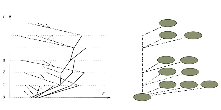
Figure 1: Embedding a CMJ individual into a multi-type GW process stemming from a single cluster of size $Z_{0}=3$. Left panel. Solid lines represent the lineages of the stem process which dies out by time $L=6$. Dashed lines delineate the daughter clusters directly generated by the stem process. We see that $X_{1}=3$ with $\tau_{1}(E)=0$, $\tau_{2}(E)=1$, $\tau_{3}(E)=3$. Right panel. The summary of the individual life: $(X_{1},\ldots,X_{L})=(3,2,2,0,2,1)$.

Throughout this paper we assume

$$f(s_{0})\in(0,\infty)\text{ for some }s_{0}>0,\text{ where }f(s)=\sum_{n=1}^{\infty}f_{n}s^{n},$$ (11)

so that on one hand, that $f_{n}>0$ for some $n\geq 1$, and on the other hand, the radius of convergence

$$r=\inf\{s\geq 0\colon f(s)=\infty\}$$

is positive. The assumption $r>0$ prohibits very fast growing sequences of the type $f_{n}=e^{n^{2}}$.

Definition 8

Given (11), define a parameter $R\in(0,\infty)$ as $R=r$ if $f(r)<1$, and as the unique positive solution of the equation $f(R)=1$ if $f(r)\geq 1$.

Since $f(R)\leq 1$, the sequence $(f_{n}R^{n})$ can be viewed as a (possibly defective) distribution on the lattice $\{1,2,\ldots\}$. This is the distribution of the inter-arrival time for the renewal process naturally embedded into the CMJ process defined above. The renewal process is interpreted as the consecutive ages at childbearing as one tracks a single ancestral lineage backwards in time. Given $f(R)=1$, the mean inter-arrival time for the embedded renewal process equals

$$\sum_{n=1}^{\infty}nf_{n}R^{n}=Rf^{\prime}(R),$$

and is interpreted as the average age at childbearing or the mean generation length for the CMJ process, see [4].

Focussing on the current waiting time of such a discrete renewal process, we get an irreducible Markov chain with the state space $\{0,1,\ldots\}$. The following observation concerning this Markov chain is straightforward.

Proposition 9

The embedded renewal process is transient if $f(r)<1$, and recurrent if $f(r)\geq 1$. Let $R$ be defined by Definition 8. If $f(r)>1$, then $R\in(0,r)$, $f^{\prime}(R)<\infty$, and the embedded renewal process is positive recurrent. If $f(r)=1$, then the embedded renewal process is either positive recurrent or null recurrent depending on whether $f^{\prime}(r)<\infty$ or $f^{\prime}(r)=\infty$.

Let $W_{n}$ be the number of newborn individuals at time $n$ in the embedded CMJ process started from a single newborn individual, or in other words, the total number of clusters emerging at time $n$ in the original GW process starting from a single cluster. Clearly,

$$F_{n} :=\mathrm{E}(W_{n})=\iint g(y)M^{n-1}(x,\mathrm{d}y)\gamma(dx).$$

Theorem 10

Consider a kernel $M$ with atom $(g,\gamma)$. Parameter $R$ from Definition 8 coincides with the convergence parameter of the kernel $M$. Moreover,

(i) if $f(r)<1$, then $R=r$, $f(R)<1$, and $F(R)<\infty$, so that $M$ is $R$-transient,

(ii) if $f(r)\geq 1$, then $f(R)=1$ and $F(R)=\infty$, so that $M$ is $R$-recurrent,

(iii) if $f(R)=1$, then either $f^{\prime}(R)=\infty$ so that $M$ is $R$-null recurrent, or $f^{\prime}(R)\in(0,\infty)$, so that $M$ is $R$-positive recurrent.

Proof. Using the law of total expectation it is easy to justify the following recursion

$$F_{n}=f_{n}+f_{n-1}F_{1}+\ldots+f_{1}F_{n-1}.$$

This leads to the equality for generating functions

$$F(s)=f(s)+f(s)F(s),$$

which yields

$$F(s)={f(s)\over 1-f(s)}\quad\text{for $s$ such that }f(s)<1.$$ (12)

From here and in view of Definition 3, it is obvious that the first statement is valid. Parts (i) and (ii) follow immediately. Part (iii) is proven in Section 5. $\Box$

Remark. For a general starting configuration of particles $Z_{0}$, putting $\mu_{0}=\mathrm{E}Z_{0}$, we get

$$\tilde{f}_{n} :=\mathrm{E}X_{n}=\iint g(y)m^{n-1}(x,dy)\mu_{0}(dx),$$

$$\tilde{F}_{n} :=\mathrm{E}Y_{n}=\iint g(y)M^{n-1}(x,\mathrm{d}y)\mu_{0}(dx).$$

The corresponding generating functions

$$\tilde{f}(s)=\sum_{n=1}^{\infty}\tilde{f}_{n}s^{n},\quad\tilde{F}(s)=\sum_{n=1}^{\infty}\tilde{F}_{n}s^{n},$$

are connected by

$$\tilde{F}(s)={\tilde{f}(s)\over 1-f(s)}\quad\text{for $s$ such that }f(s)<1.$$ (13)

(To obtain this relation, observe that

$$\tilde{F}_{n}=\tilde{f}_{n}+\tilde{f}_{n-1}F_{1}+\ldots+\tilde{f}_{1}F_{n-1},$$

which gives $\tilde{F}(s)=\tilde{f}(s)(1+F(s))$, and it remains to apply (12).)

As mentioned above, under the special initial condition $Z_{0}\stackrel{{\scriptstyle d}}{{=}}\tau$, the embedded CMJ process starts from a single newborn individual. For a general $Z_{0}$, the embedded CMJ process has an immigration component characterised by the generating function $\tilde{f}(s)$. By immigration we mean the inflow of new clusters generated by the stem process starting from $Z_{0}$ particles.

5 Null and positive recurrence of a kernel with atom

Consider a non-negative kernel $M$ with atom $(g,\gamma)$, and put

$$M_{s}(x,A)=\sum_{n=1}^{\infty}s^{n}M^{n-1}(x,A),\quad m_{s}(x,A)=\sum_{n=1}^{\infty}s^{n}m^{n-1}(x,A),\quad s\geq 0,$$

so that the earlier introduced generating functions $F$ and $f$ can be presented as

$$F(s)=\iint g(y)M_{s}(x,\mathrm{d}y)\gamma(\mathrm{d}x),\quad f(s)=\iint g(y)m_{s}(x,\mathrm{d}y)\gamma(\mathrm{d}x).$$

Denote

$$h_{s}(x)=\int g(y)m_{s}(x,\mathrm{d}y),\qquad\pi_{s}(A)=\int m_{s}(x,A)\gamma(\mathrm{d}x),$$ (14)

and observe that

$$\int h_{s}(x)\gamma(\mathrm{d}x)=\int g(y)\pi_{s}(\mathrm{d}y)=f(s),\quad\int h_{s}(y)\pi_{s}(\mathrm{d}y)=s^{2}f^{\prime}(s).$$

The latter equality requires the following argument

$$\int h_{s}(x)\pi_{s}(\mathrm{d}x) =\iiint g(y)m_{s}(x,\mathrm{d}y)m_{s}(z,\mathrm{d}x)\gamma(\mathrm{d}z)$$

$$=\iint g(y)m_{s}^{2}(z,\mathrm{d}y)\gamma(\mathrm{d}z)=\sum_{n=1}^{\infty}ns^{n+1}f_{n}=s^{2}f^{\prime}(s),$$

where we used the relation

$$s^{-2}m_{s}^{2}(y,A) =\int s^{-1}m_{s}(x,A)s^{-1}m_{s}(y,\mathrm{d}x)=\sum_{n=0}^{\infty}\sum_{k=0}^{\infty}\int s^{n}m^{n}(x,A)s^{k}m^{k}(y,\mathrm{d}x)$$

$$=\sum_{n=0}^{\infty}\sum_{k=0}^{\infty}s^{n+k}m^{n+k}(y,A)=\sum_{j=0}^{\infty}(j+1)s^{j}m^{j}(y,A).$$

Lemma 11

Consider a kernel with atom (5). If a positive $s$ is such that $f(s)\leq 1$, then the function $h_{s}$ and the measure $\pi_{s}$, defined by (14), satisfy

$$\int h_{s}(y)M(x,\mathrm{d}y) =s^{-1}h_{s}(x)-(1-f(s))g(x),$$ (15)

$$\int M(y,A)\pi_{s}(\mathrm{d}y) =s^{-1}\pi_{s}(A)-(1-f(s))\gamma(A),$$ (16)

so that they are $s$-subinvariant function and measure for the kernel $M$.

Proof. By (5), we have

$$\int m_{s}(y,A)M(x,\mathrm{d}y) =\sum_{n=1}^{\infty}s^{n}m^{n}(x,A)+g(x)\int m_{s}(y,A)\gamma(\mathrm{d}y)$$

$$=s^{-1}m_{s}(x,A)-\delta_{x}(A)+g(x)\pi_{s}(A),$$

which implies relation (15):

$$\int h_{s}(y)M(x,\mathrm{d}y) =\iint g(w)m_{s}(y,\mathrm{d}w)M(x,\mathrm{d}y)=s^{-1}h_{s}(x)-g(x)+g(x)f(s).$$

Similarly, from

$$\int M(y,A)m_{s}(x,\mathrm{d}y) =\sum_{n=1}^{\infty}s^{n}m^{n}(x,A)+\gamma(A)\int g(y)m_{s}(x,\mathrm{d}y)$$

$$=s^{-1}m_{s}(x,A)-\delta_{x}(A)+\gamma(A)h_{s}(x),$$

we arrive at relation (16). $\Box$

Lemma 11 yields the following statement which in turn provides the proof of part (iii) of Theorem 10 (recall Definition 5).

Corollary 12

Consider an $R$-recurrent kernel $M$ with atom $(g,\gamma)$. If $f(R)=1$, then $h=h_{R}$ and $\pi=\pi_{R}$ are $R$-invariant function and measure satisfying relation (7) with $n_{0}=1$, relation (8), as well as

$$\int h(y)\pi(\mathrm{d}y)=R^{2}f^{\prime}(R).$$

Observe that

$$h(x)=\sum_{n=1}^{\infty}R^{n}\int g(y)m^{n-1}(x,dy)$$ (17)

is the expected $R$-discounted number of clusters ever produced by the stem process starting from a single particle of type $x$. From this angle, $h(x)$ can be interpreted as the reproductive value of type $x$. On the other hand,

$$\pi(A)=\sum_{n=1}^{\infty}R^{n}\int m^{n-1}(x,A)\gamma(\mathrm{d}x).$$ (18)

is the expected $R$-discounted number of particles whose type belongs to $A$ and which appear in the stem process starting from a single cluster of particles. As shown next, see Theorem 13, the measure $\pi$ can be viewed as an asymptotically stable distribution for the types of particles in the GW process with clusters.

6 Perron-Frobenius theorem for kernels with atom

Theorem 13

Consider an aperiodic $R$-positive recurrent kernel $M$ with atom $(g,\gamma)$. Let $h$ and $\pi$ be given by (17) and (18). If $(x,A)$ are such that

$$R^{n}m^{n}(x,A)\to 0,\quad n\to\infty,$$ (19)

then

$$R^{n}M^{n}(x,A)\to\dfrac{h(x)\pi(A)}{R^{2}f^{\prime}(R)},\quad n\to\infty.$$ (20)

If $h(x)<\infty$, then condition (19) holds for any $A$ such that

$$A\subset\{y:g(y)\geq\epsilon\}\text{ for some }\epsilon>0.$$ (21)

To prove this result we need two lemmas. In the end of this section we give a remark addressing condition (19).

Lemma 14

Consider a kernel $M$ with atom $(g,\gamma)$. If $s>0$ is such that $f(s)<1$, then

$$M_{s}(x,A) =m_{s}(x,A)+{h_{s}(x)\pi_{s}(A)\over 1-f(s)}\quad\text{for all }x\in E,A\in\mathcal{E}.$$ (22)

Proof. By (5), we have the recursion

$$M^{n}(x,A) =g(x)\int M^{n-1}(y,A)\gamma(\mathrm{d}y)+\int M^{n-1}(y,A)m(x,\mathrm{d}y)$$

$$=g(x)\int M^{n-1}(y,A)\gamma(\mathrm{d}y)+\int g(y)m(x,\mathrm{d}y)\int M^{n-2}(z,A)\gamma(\mathrm{d}z)$$

$$\quad+\int M^{n-2}(z,A)m^{2}(x,dz)$$

$$=\sum_{i=1}^{n}\int g(y)m^{i-1}(x,\mathrm{d}y)\int M^{n-i}(y,A)\gamma(\mathrm{d}y)+m^{n}(x,A),$$

which in terms of generating functions gives

$$M_{s}(x,A) =m_{s}(x,A)+h_{s}(x)\int M_{s}(y,A)\gamma(\mathrm{d}y),$$

and after integration,

$$\int M_{s}(x,A)\gamma(\mathrm{d}x) ={\pi_{s}(A)\over 1-f(s)}.$$

Combining the last two relations we get (22). Observe also that the last formula yields (12).

$\Box$

Lemma 15

Let

$$a(s)=\sum_{n=0}^{\infty}a_{n}s^{n},\quad b(s)=\sum_{n=0}^{\infty}b_{n}s^{n},\quad c(s)=\sum_{n=0}^{\infty}c_{n}s^{n},$$

be three generating functions for non-negative sequences connected by

$$c(s)={b(s)\over 1-a(s)}.$$

If sequence $\{a_{n}\}$ is aperiodic with $a(1)=1$, $a^{\prime}(1)\in(0,\infty)$, then

$$c_{n}\to\dfrac{b(1)}{a^{\prime}(1)},\quad n\to\infty.$$

Proof. This is a well-known result from Chapter XIII.4 in [3]. $\Box$

Proof of Theorem 13. $R$-positive recurrence implies $f(R)=1$ and $f^{\prime}(R)\in(0,\infty)$. Due to $f(R)=1$, we can rewrite (22) as

$$M_{\hat{s}}(x,A)-m_{\hat{s}}(x,A)={b(s)\over 1-a(s)},$$

where $\hat{s}=sR$ and

$$a(s)=f(sR),\quad b(s)=h_{\hat{s}}(x)\pi_{\hat{s}}(A),$$

so that $a^{\prime}(1)=Rf^{\prime}(R)$, $b(1)=h(x)\pi(A)$. Applying Lemma 15, we find that as $n\to\infty$,

$$R^{n}(M^{n}(x,A)-m^{n}(x,A))\to\dfrac{h(x)\pi(A)}{R^{2}f^{\prime}(R)}.$$

which combined with condition (19) yields the main assertion. The stated sufficient condition for (19) is verified using

$$\sum_{n=1}^{\infty}R^{n}m^{n-1}(x,A)\leq\sum_{n=1}^{\infty}R^{n}\int 1_{\{y:g(y)>\epsilon\}}m^{n-1}(x,dy)\leq\epsilon^{-1}h(x)<\infty.$$

$\Box$

Remark. To illustrate the role of the condition (19), consider the kernel (5) with

$$m(x,A)=g_{1}(x)\gamma_{1}(A),$$

assuming

$$\int g_{1}(x)\gamma_{1}(dx)=a_{1},\quad\int g(x)\gamma(dx)=a,\quad\int g_{1}(x)\gamma(dx)=\int g(x)\gamma_{1}(dx)=0,$$

where $a_{1}>a>0$. In this particular case, we have

$$M^{n}(x,A)=m^{n}(x,A)+a^{n}g(x)\gamma(A),\quad m^{n}(x,A)=a_{1}^{n}g_{1}(x)\gamma_{1}(A),$$

and clearly,

$$M^{n}(x,A)\sim\left\{\begin{array}[]{ll}a_{1}^{n}g_{1}(x)\gamma_{1}(A),&\text{if }g_{1}(x)\gamma_{1}(A)>0,\\ a^{n}g(x)\gamma(A),&\text{if }g_{1}(x)\gamma_{1}(A)=0\text{ and }g(x)\gamma(A)>0.\end{array}\right.$$

Turning to the generating function defined by (6) we find

$$F_{n}=\iint g(y)M^{n-1}(x,\mathrm{d}y)\gamma(dx)=a^{n+1},\quad F(s)={a^{2}s\over 1-as}.$$

This yields $R=a^{-1}$ and we see that condition (19) is not valid for $(x,A)$ such that $g_{1}(x)\gamma_{1}(A)>0$. On the other hand, if $g(x)<\infty$ and $A$ satisfies (21), then

$$0=\int g(x)\gamma_{1}(dx)\geq\int_{A}g(x)\gamma_{1}(dx)\geq\epsilon\gamma_{1}(A),$$

so that $\gamma_{1}(A)=0$ and therefore $R^{n}M^{n}(x,A)\to g(x)\gamma(A)$.

7 3-parameter GW process with clusters

Here we construct a transparent example of a GW process with clusters having the type space $E=[0,\infty)$. Its positive recurrent reproduction kernel is fully specified by just three parameters $a,c\in(0,\infty)$, and $b\in(-1,\infty)$:

$$M(x,\mathrm{d}y)=ae^{x-y}1_{\{y\geq x\}}\mathrm{d}y+ce^{-bx}\delta_{0}(\mathrm{d}y).$$

This kernel satisfies (5) with

$$m(x,\mathrm{d}y)=ae^{x-y}1_{\{y\geq x\}}\mathrm{d}y,\quad g(x)=ce^{-bx},\quad\gamma(A)=\delta_{0}(A),$$ (23)

implying that each cluster consists of a single particle of type 0.

The full specification of our example refers to a continuous time Markov branching process modeling the size of a population of Markov particles having the unit life-length mean and offspring mean $a$. The main idea is to count the Markov particles generation-wise, and to define the type of a Galton-Watson particle as the birth-time of the corresponding Markov particle. The corresponding stem process $\{\xi_{n}\}_{n\geq 0}$ is defined by

$\xi_{n}(A)=$ the number of $n$-generation Markov particles born in the time period $A$,

so that its conditionally on the parent’s birth time $x$,

$$m^{n}(x,[0,t])=a^{n}\mathbb{P}(x+T_{1}+\ldots+T_{n}\leq t)=a^{n}\mathbb{P}(N_{t-x}\geq n),\quad\text{for }t>x,$$

where $T_{i}$ are independent exponentials with unit mean and $\{N_{t}\}_{t\geq 0}$ is the standard Poisson process.

Proposition 16

Consider the above described multi-type GW process with clusters characterised by (23). Then we have

$$f(s)={rcs\over r-s},\qquad r={1+b\over a},\qquad R={r\over 1+cr}.$$ (24)

The process is supercritical if $c>{r-1\over r}$, critical if $c={r-1\over r}$, and subcritical if $c<{r-1\over r}$.

Convergence (20) holds for $A=[0,t]$, $t\in[0,\infty)$, with the right hand side equal to

$$e^{-bx}(R\delta_{0}(\mathrm{d}y)+aR^{2}e^{(aR-1)y}\mathrm{d}y).$$

If $Ra<1$, then (20) holds even for $A=E$ with the right hand side equal to ${Re^{-bx}\over 1-aR}$.

Proof. Referring to the underlying Poisson process, we find that for $s\neq 1/a$,

$$m_{s}(0,[0,t]) =s\sum_{n=0}^{\infty}s^{n}a^{n}\sum_{k=n}^{\infty}\mathbb{P}(N_{t}=k)=s\sum_{k=0}^{\infty}\mathbb{P}(N_{t}=k){1-(as)^{k+1}\over 1-as}$$

$$={s\over 1-as}(1-as\mathbb{E}(as)^{N_{t}})={s\over 1-as}(1-ase^{t(as-1)}).$$

More generally, we have

$$m_{s}(x,[0,t])=m_{s}(0,[0,t-x])={s\over 1-as}(1-ase^{(t-x)(as-1)})1_{\{t\geq x\}},$$

so that

$$m_{s}(x,\mathrm{d}y)=s\delta_{x}(\mathrm{d}y)+as^{2}e^{(as-1)(y-x)}1_{\{y\geq x\}}\mathrm{d}y.$$

By (14)

$$h_{s}(x)=\int g(y)m_{s}(x,\mathrm{d}y)=sce^{-bx}+cas^{2}\int_{0}^{\infty}e^{h(as-1)}e^{-b(x+u)}du=f(s)e^{-bx},$$

where $f(s)$ satisfies (24). Since $f(r)=\infty$, the stated value $R={r\over 1+cr}$ is found from the equation $f(R)=1$.

Applying once again (14), we find

$$\pi_{s}(\mathrm{d}y)=\int m_{s}(x,\mathrm{d}y)\gamma(\mathrm{d}x)=m_{s}(0,\mathrm{d}y)=s\delta_{0}(\mathrm{d}y)+as^{2}e^{(as-1)y}\mathrm{d}y.$$

To check this and previously obtained expressions, we verify the general formula for the integral

$$\int h_{s}(x)\pi_{s}(\mathrm{d}x) =sf(s)+f(s)as^{2}\int e^{-(1+b)x}e^{asx}\mathrm{d}x={rsf(s)\over r-s}={r^{2}s^{2}\over(r-s)^{2}}=s^{2}f^{\prime}(s).$$

With

$$h(x) =e^{-bx},\qquad\pi(\mathrm{d}x)=R\delta_{0}(\mathrm{d}x)+aR^{2}e^{(aR-1)x}\mathrm{d}x,$$

Theorem 13 specialised to the current example says that for $t\in[0,\infty)$,

$$R^{n}M^{n}(x,[0,t]) \to e^{-bx}(R+aR^{2}\int_{0}^{t}e^{(aR-1)y}\mathrm{d}y)$$

$$=e^{-bx}(R+{aR^{2}\over aR-1}(e^{(aR-1)t}-1))=e^{-bx}{aR^{2}e^{(aR-1)t}-R\over aR-1},\quad n\to\infty.$$

If $aR<1$ and $A=E$, then condition (19) holds since

$$\pi(E)=R+{aR^{2}\over 1-aR}={R\over 1-aR}<\infty,$$

and $R^{n}m^{n}(x,E)=(Ra)^{n}\to 0$. $\Box$

Remark. If we further specialize this example by letting the stem process to be the Yule process, then we have $a=2$. If furthermore, $b=2$ and $c<{r-1\over r}={1\over 3}$, then the corresponding GW process with clusters is subcritical, despite the total number of particles in the Yule process is infinite.

Acknowledgements. The author is grateful for critical remarks of an anonymous reviewer of an earlier version of the paper.

References

[1]Athreya, K. and Ney, P. (1972) Branching processes, John Wiley & Sons, London-New York-Sydney.
[2]Athreya, K. and Ney, P. (1982) A Renewal Approach to the Perron-Frobenius Theory of Non-negative Kernels on General State Spaces.
Mathematische Zeitschrift 179, 507–530.
[3]Feller, W. (1959). An introduction to probability theory and its applications, Vol I, 2nd ed. John Wiley & Sons, London-New York-Sydney.
[4]Jagers, P. (1975) Branching processes with biological applications, Wiley, New-York.
[5]Jagers, P. and Sagitov, S. (2008) General branching processes in discrete time as random trees. Bernoulli 14, 949–962.
[6]Harris, T. E. (1963) The Theory of Branching Processes, Springer, Berlin.
[7]Lindo, A. and Sagitov, S. (2018) General linear-fractional branching processes with discrete time. Stochastics90, 364–378.
[8]Mode, C.J. (1971) Multitype branching processes: theory and applications.
Volym 34 av Modern analytic and computational methods in science and mathematics. American Elsevier Pub. Co.,
[9]Olofsson, P. (1996) Branching processes with local dependencies. Ann. Appl. Probab. 6, 238–268.
[10]Nummelin, E. (1984) General Irreducible Markov Chains and Non-negative Operators, Cambridge University Press, London.
[11]Sagitov, S. (2013) Linear-fractional branching processes with countably many types. Stoch. Proc. Appl. 123, 2940–2956.