Panchromatic Hubble Andromeda Treasury. XIX. The Ancient Star Formation History of the M31 Disk

Abstract

We map the star formation history across M31 by fitting stellar evolution models to color-magnitude diagrams of each 83${}^{\prime\prime}{\times}83^{\prime\prime}$ (0.3$\times$1.4 kpc, deprojected) region of the PHAT survey outside of the innermost 6${}^{\prime}{\times}12^{\prime}$ portion. We find that most of the star formation occurred prior to $\sim$8 Gyr ago, followed by a relatively quiescent period until $\sim$4 Gyr ago, a subsequent star formation episode about 2 Gyr ago and a return to relative quiescence. There appears to be little, if any, structure visible for populations with ages older than 2 Gyr, suggesting significant mixing since that epoch. Finally, assuming a Kroupa IMF from 0.1$-$100 M_⊙, we find that the total amount of star formation over the past 14 Gyr in the area over which we have fit models is 5${\times}$10¹⁰ M_⊙. Fitting the radial distribution of this star formation and assuming azimuthal symmetry, (1.5$\pm$0.2)${\times}$10¹¹ M_⊙ of stars have formed in the M31 disk as a whole, (9$\pm$2)${\times}$10¹⁰ M_⊙ of which has likely survived to the present after accounting for evolutionary effects. This mass is about one fifth of the total dynamical mass of M31.

1. Introduction

While large disk galaxies are responsible for the majority of star formation in the universe (Freeman & Bland-Hawthorn, 2002; Bell et al., 2005), the details of their formation and evolution are difficult to constrain with observations. They are complex, having a wide range of stellar populations, multiple structural components, and complicated dust distributions. Although they are the most common galaxies in large surveys, integrated light studies of disks from such surveys are generally limited to their global properties, component structures, and environments (e.g., Tremonti et al., 2004; MacArthur et al., 2004; Blanton & Moustakas, 2009, and many others). While these measurements are important for statistical comparisons, only by resolving the individual stars within a galaxy can we reliably map the stellar populations that are the products of its entire evolutionary history. In particular, the resolved stars probe the star formation history (SFH), which provides the age, mass, and metallicity distributions of the galaxy’s constituent stars. These fundamental quantities allow detailed comparisons with numerical simulations and stringent tests of our ability to infer the masses, metallicities, and star formation rates of distant galaxies from integrated light measurements.

M31 provides the best opportunity to measure the resolved stellar populations of a large disk galaxy outside of the Milky Way. At 770 kpc (McConnachie et al., 2005), we can resolve M31’s individual stars to below the horizontal branch with HST. M31 is therefore the only large, metal-rich disk galaxy whose SFH can be accurately measured and mapped. However, M31’s large angular size and complex dust distribution have made it difficult to disentangle its stellar populations. There are many studies in the literature (e.g., Williams, 2002; Bellazzini et al., 2003; Williams, 2003; Brown et al., 2003, 2009; Williams et al., 2009; Bernard et al., 2012, 2015b, 2015a; Williams et al., 2015), but most have been forced to limit their work to small areas or to the outskirts of the disk where dust obscuration is minimal. This work has provided significant insight, including the complexity of the halo populations (Brown et al., 2003) and the first clues that the star formation rate in M31 has decreased significantly over the past $\sim$Gyr (Williams, 2002). Results from these deep drilling fields, however, have been difficult to incorporate into a global picture of the complex galaxy.

Over the past few decades, fitting resolved stellar photometry to measure SFHs has become a powerful tool for constraining galaxy formation and evolution. For example, great strides have been made in understanding the characteristics and evolution of dwarf galaxies through such measurements (e.g., Mateo, 1998; Dohm-Palmer et al., 2002; Gallart et al., 2005; Dolphin et al., 2005; Young et al., 2007; Cole et al., 2007; Weisz et al., 2011; Skillman et al., 2014, 2017, and many others). These SFHs allow us to test models with detailed observational constraints. Because of this, the technique of using resolved stars to constrain SFHs has revolutionized the study of dwarf galaxies in the Local Group and beyond. Unfortunately, due to their greater complexity, size, and distance to the nearest examples, it has proven difficult to apply this powerful tool to large disks rather than dwarf galaxies. Stellar population studies of our own Galaxy are compromised by dust in the Galactic plane.

Recently, the PHAT survey has begun to shed light on the global SFH of M31 by fitting resolved stellar photometry. Lewis et al. (2015) provided spatially-resolved measurements of the recent SFH over the past 500 Myr using the optical photometry from PHAT. They found M31’s major star forming ring is a very long-lived structure in the M31 disk. At older ages in selected low-dust regions, Williams et al. (2015) found that the star formation episode at $\sim$2-4 Gyr ago, previously detected in the stellar populations of the outer parts of M31 (Bernard et al., 2015b), is also seen all the way in to just a few kpc from the galaxy center, suggesting the intense event in the history of M31 causing this burst in star formation was felt all the way to the inner disk. Intriguingly, this episode appears relatively weak in the southern disk (Bernard et al., 2015a), although their SFHs show somewhat enhanced rates at these ages as well.

Combining the complete areal coverage of the Lewis et al. (2015) recent SFH maps with the deep analysis of ancient SFHs from Williams et al. (2015) requires a new approach to handle M31’s complex distribution of dust. Not only must the SFH be measured independently in each subregion of the disk, the dust must be measured and modeled properly at each position as well.

In this paper, we produce the first wide-area maps of the full SFH of the M31 disk. These maps cover all but the innermost area of the PHAT footprint (which is too crowded for this work). Section 2 details the data analysis techniques used to model the dust and stellar populations when measuring M31’s SFH. Section 3 provides our resulting SFHs electronic tables, FITS images, and movies to show the time-resolved build-up of the current stellar mass distribution of the PHAT footprint of M31. A companion paper (Williams et al., in preparation) will discuss the resulting map of stellar mass, along with the resulting spatially-resolved mass-to-light ratio relations for M31. Throughout the paper, we assume a distance modulus for M31 of 24.47 (McConnachie et al., 2005). The nominal foreground extinction is $A_{\rm VFG}=0.17$ (Schlafly & Finkbeiner, 2011).

2. Data Analysis

The data for this study come from the Panchromatic Hubble Andromeda Treasury (PHAT; Dalcanton et al., 2012; Williams et al., 2014). Briefly, PHAT is a multiwavelength HST survey mapping 414 contiguous HST fields of the northern M31 disk and bulge in 6 broad wavelength bands from the near-ultraviolet to the near-infrared. The broad wavelength coverage required that the region be covered with 3 HST detectors. The survey obtained data in the F275W and F336W bands with the UVIS detectors of the WFC3 camera, the F475W and F814W bands in the WFC detectors of the ACS camera, and the F110W and F160W bands in the IR detectors of the WFC3 camera.

For this work, we use the photometry and artificial star tests provided in Williams et al. (2014), as well as the dust extinction maps from Dalcanton et al. (2015), to fit for the SFH of $83^{\prime\prime}{\times}83^{\prime\prime}$ subregions of the survey area. The methods for producing these catalogs and maps are described in detail in Williams et al. (2014) and Dalcanton et al. (2015), respectively. The data are homogeneous in exposure time in each band over the survey, but they vary significantly in photometric depth and precision due to crowding effects. In Figure 1, we provide a map of the stellar density of bright stars with 18.5$<$m${}_{F160W}{<}$19.5, for which the PHAT survey is complete at all stellar densities. This metric results in a smooth distribution of stellar densities over the PHAT survey area. Figures 2, 3, and 4 show example color-magnitude diagrams (CMDs), completeness limits, and photometric uncertainties for a range of stellar densities show in the map in Figure 1. A more detailed discussion of how these measurements were made is provided in Williams et al. (2014). We show examples here to demonstrate the wide range of photometric quality over the survey area.

As the photometric analysis is detailed in Williams et al. (2014), we focus here on the additional analysis necessary to measure spatially-resolved ancient star formation histories from these data, in particular, fitting models to the PHAT photometry. We use the software package MATCH 2.6 (Dolphin, 2002, 2012, 2013) to find the combination of model stellar ages and metallicities that best fit the CMD of each sample of stars brighter than the 50% completeness limit. This software package has been well tested and proven to provide reliable measurements (e.g., Dolphin et al., 2005; Williams et al., 2009; McQuinn et al., 2010; Williams et al., 2011; Weisz et al., 2011; Cole et al., 2014; Williams et al., 2015, and many others).

We use this package in a similar way to these studies, comparing results when fitting with the Padova (Marigo et al., 2008; Girardi et al., 2010) models to those from fitting with the PARSEC (Bressan et al., 2012), BaSTI (Pietrinferni et al., 2004; Cassisi et al., 2006; Pietrinferni et al., 2013), and MIST (Choi et al., 2016) models. In addition, testing fits with different models allows us to assess the uncertainties (and ultimately the reliability) associated with these late stages of evolution upon which most of our measurements depend. In Figure 5, we show comparison CMDs of these models in F475W-F814W, shifted to the distance of M31, at 2 ages (2 and 10 Gyr) and 2 metallicities ([Fe/H]=$-$1.0 and 0.0). For comparisons with other relevant ages, we plot isochrones of 1, 2, 4, and 10 Gyr in the figure as well. There are significant differences in feature color and shape, especially in the red clump, sub-giant branch and RGB. One well known difference between these model sets is that the BaSTI set has an extended horizontal branch (HB) and the other sets do not. There is very little evidence for an extended HB in the PHAT photometry outside of the bulge and minor-axis fields (Rosenfield et al., 2012; Williams et al., 2012), and the feature is so weak compared to the red clump and red-giant branch that our results depend very little on it.

The shape and position of the red clump is very sensitive to age and metallicity (e.g., Rejkuba et al., 2005; Williams et al., 2009). With the age-metallicity relation fixed, the age distribution plays a strong role in the ability to match this feature. Slight differences in the color and brightness of the red clump as a function of age in different model sets therefore can significantly affect the age distribution. The Padova and PARSEC models come from the same research group and have similar red clumps, whereas the others are different. Thus, our uncertainty at these ages in any one set of fits is large, and there could be systematic differences between the results of the innermost regions ($<$5 kpc), where the red clump stars cannot be measured, and the rest of the PHAT footprint (see § 3.4). Adopting long time bins at old ages, as we have done, helps to account for these uncertainties and improves the consistency of the results across these different model sets.

Our data are more complicated than those typically fit using MATCH. We have more than 2 observed bands, covering a wide range of depth and crowding, and a very complex dust distribution. Below we describe the details of the CMD modeling, which takes advantage of many powerful tools that MATCH provides, including sophisticated dust extinction models, simultaneous fitting of multiple CMDs, and the ability to force a chemical enrichment history.

2.1. Artificial Star Tests

The PHAT survey covers over 800 HST fields of M31, which presents a daunting computational problem when trying to characterize the photometric biases by analyzing the recovery of artificial stars. As a compromise, Williams et al. (2014) only performed artificial star tests at 6 representative positions along the major axis. These tests were enough to characterize the photometric quality as a function of stellar density, but were not comprehensive as they did not sample every location in the survey.

To fit the CMDs over the entire survey area with MATCH as described in detail in Williams et al. (2014), it was necessary to insert and recover artificial stars to measure the bias, uncertainty, and completeness of the photometry as a function of color and magnitude at every location in the survey. As shown in Williams et al. (2014), the stellar density varies dramatically from the dense inner bulge to the diffuse outer disk in spite of the equal exposure times. Given this density spread, spatial variation in photometric quality, biases and depth are completely dominated by variations in the density of stars (i.e., crowding). We therefore use stellar density as an indicator of the expected crowding in each region. We therefore use stellar density (i.e., Figure 1) as an indicator of the expected crowding in each region.

For each stellar density sampled in Williams et al. (2014), we measured the bias, skew, variance, and covariance in the differences between the input and output magnitudes of the artificial stars in Williams et al. (2014) as well as the probability that a star is recovered (completeness). We then characterize these quantities in 0.05 mag $\times$ 0.05 mag color-magnitude bins. These parameters all follow smooth relationships when plotted against the density of bright stars with 18.5$<$m${}_{F160W}{<}$19.5. We therefore fit curves to these quantities, and used the fitted values to derive bias, skew, variance, covariance and completeness values for each color, magnitude, and stellar density in the PHAT survey.

Using the fits to the artificial star results, we can simulate the properties of artificial star tests in every survey region. We generated simulated artificial star catalogs for each of the $83^{\prime\prime}{\times}83^{\prime\prime}$ regions in our study based on the density of stars, where the simulated fake star catalogs used as inputs to MATCH are created to have the bias, skew, variance, covariance, and completeness matched to the stellar density of the region.

We tested the efficacy of our manufactured fake star catalogs by running SFH fits with MATCH for both the actual fake star tests, as well as with our simulated fake star tests in one of the 6 regions from Williams et al. (2015) where we had both. The resulting SFHs are shown in Figure 6. Here, the gray shaded areas mark the $\sim$1$\sigma$ random uncertainties from each fit (see Section 2.3 for uncertainty determination). The results agree to well within these random uncertainties.

2.2. Fitting

Although MATCH has been extensively tested and used for SFH measurements in the literature, there were aspects of the PHAT photometry that required us to use relatively new capabilities of the software. In what follows, we describe our methods for applying these capabilities for extinction, chemical enrichment, multi-band photometry, and uncertainty determination.

2.2.1 Extinction Modeling

An extremely challenging aspect to measuring the ancient SFH of the M31 disk is proper modeling of its complex dust extinction. Across the PHAT survey, the range of crowding effects and differential extinction effects are noticeable. Crowding causes fewer faint stars to be detected at high stellar densities, and it causes the CMD features to be broader (Williams et al., 2014). Differential extinction also broadens the features, but only along the reddening vector. As can be seen clearly at lower stellar densities where the features are well-defined, the red giant branch and red clump are split into a reddened component behind the dust and a foreground component in front of the dust. This difference in the effects of crowding and reddening allowed the IR data to be used for the extinction mapping in Dalcanton et al. (2015), and it also allows us to fit the CMD features to obtain reliable estimates of the age and metallicity distribution of the stars, as described below.

Dalcanton et al. (2015) made a major innovation in our ability to model the differential extinction in the M31 disk. They found that the spread in reddening of red giant branch stars in the PHAT survey, if taken over small spatial areas, had two components: an unreddened component and a reddened component. Further, the reddened component was well-represented by a log-normal distribution with the following parameterization: the median $A_{\rm V}$ ($\mu$), the dimensionless width of the log-normal $A_{\rm V}$ distribution ($\sigma$), and the fraction of stars being affected by the dust (f_red). They used these parameters to produce the most detailed and comprehensive map of the dust distribution of the M31 disk to date.

In order to use these maps for our fitting, we needed to degrade the very fine resolution of the Dalcanton et al., 2015 maps. Due to internal dynamics and interactions, the old populations ($\;\buildrel>\over{\sim}\;$1 Gyr) should be well-mixed on spatial scales much larger than the Dalcanton et al. (2015) pixel scale. Furthermore, the number of stars in these small regions is too low to provide good statistics for SFH fitting. Fortunately, we were able to develop a way to combine pixels in the Dalcanton et al. (2015) maps to allow larger samples of stars to be fitted simultaneously using sums of log-normal distributions, which we describe below.

We began with the Dalcanton et al. (2015) extinction maps, which are on a 3.3^′′ (13 pc) pixel^-1 scale. We took stellar photometry from each of these $3.3^{\prime\prime}{\times}3.3^{\prime\prime}$ regions separately. For each of these samples, we know the correct differential extinction distribution from the Dalcanton et al. (2015) measurements. Next, we combined the $3.3^{\prime\prime}{\times}3.3^{\prime\prime}$ regions into $83^{\prime\prime}{\times}83^{\prime\prime}$ regions ($25{\times}25$ extinction map pixels) across the survey. However, each of these areas contained 625 extinction distributions in the extinction maps, and the wide range in $\mu$ and $\sigma$ values present results in a combined reddening distribution that no longer resembles our log-normal model (see Figure 7). Therefore, some subdivision of the sample in each $83^{\prime\prime}{\times}83^{\prime\prime}$ region was required.

In order to effectively apply our differential extinction model, we divided each set of 625 extinction distributions into quartiles of A_V. Once this division was done, the reddening distribution within each quartile resembled a single log-normal (see Figure 7). We then fit that log-normal to determine the parameters of the reddening distribution for that quartile of that region. Examples of fits to an unranked 625 pixel region and to a single quartile of the same sub-region are shown in Figure 7. Within each $83^{\prime\prime}{\times}83^{\prime\prime}$ region, we assigned each star to an extinction quartile based on its location in the Dalcanton et al. (2015) maps. This technique resulted in 826 regions, each with 4 photometric subsamples (one for each quartile in extinction space), each of which could be analyzed independently using the reddening distribution appropriate for that quartile. The individual quartiles typically contained 10000 to 50000 stars.

Another major milestone in our modeling ability was including this log-normal extinction distribution parameterization into MATCH. As of MATCH 2.5, in addition to applying foreground reddening to model CMDs, one can apply the $diskav$ option to convolve model CMDs with an additional log-normal extinction distribution identical to those measured in the Dalcanton et al. (2015) maps. The log-normal is applied to the fraction of RGB stars behind the M31 disk, which is also measured in the Dalcanton et al. (2015) maps.

The $diskav$ dust model in MATCH has 7 parameters. The three parameters that control the redistribution of stars in the RGB are the parameters of the log-normal reddening distribution ($\mu$, $\sigma$, and f_red). These three we take directly from the processing of the Dalcanton et al. (2015) dust maps described above. The other 4 parameters include: 1) a parameter that allows for differential foreground extinction that affects all stars, but since our regions are very small on the sky, this parameter is zero for our study; 2) three parameters that allow the young stars (less than the transition age) to have a larger fraction of stars affected by dust than old stars. One of the three is the ratio of the scale height of the young stars to the dust, another is the ratio of the scale height of the old stars to the dust, and the last is the age at which this transition occurs. We ran many hundreds of tests covering a large grid of values for the scale height and transition age parameters, and we compared the resulting fit values for these tests to determine which parameters provided the best fits. We found that 1) within a relatively broad range, the resulting ancient SFH was essentially unaffected by our choice of these parameters (the differences in fit quality were very small) and 2) the best fits were typically those with a low transition age parameter ($\sim$0.1 Gyr) and high values for the scale heights of the old stars to the dust (10-20). We thus fixed these parameters to 0.1 and 20 for all locations.

The only free reddening parameter in the fitting was the foreground extinction, which we will call $A_{\rm VFG}$ to distinguish it from $A_{\rm V}$ that we obtain from the Dalcanton et al. (2015) maps, applied to the entire CMD. This value was not constrained by Dalcanton et al. (2015), as all of their measurements were done relative to the “unreddened” component of the RGB at each location. However, these “unreddened” stars are likely to still be reddened by foreground dust in the Galaxy and/or by dust in M31 that was not fully accounted for in the dust model. We compensate for this unknown component in the extinction in MATCH by applying a extinction value $A_{\rm VFG}$ to all stars in the CMD. When fitting each sample, we limited the range to $0.1{<}A_{\rm VFG}{<}0.7$, which is reasonable given the nominal foreground value of $A_{\rm VFG}=0.17$ (Schlafly & Finkbeiner, 2011). Including this single free extinction parameter in our fitting improved the fits tremendously, making the relative likelihoods (as determined from the Poisson $-ln(p)$ value) hundreds of orders of magnitude larger than fits that did not contain this parameter or fixed it to the same value for the entire survey.

2.2.2 Enrichment Modeling

When fitting each $A_{\rm V}$ quartile of each $83^{\prime\prime}{\times}83^{\prime\prime}$ region of the PHAT photometry, we fixed the chemical evolution model used by the fitting software. For data of the depth in PHAT, jointly constraining the chemical enrichment history and star formation rate history is particularly challenging and must be treated carefully.

Given that our data quality required us to limit the freedom of the fitting routine, we decided on limiting the fitting to follow a sensible chemical evolution model. To determine an appropriate model, we started by fitting the data assuming several different potential chemical enrichment histories. Most SFH fitting work to date has focused on dwarf galaxies, and because such dwarfs are relatively simple systems, forcing simple monotonically increasing age-metallicity relations during the fitting of shallower data sets has been very successful (e.g., Weisz et al., 2011). We tried these relations (constant metallicity, constant enrichment rate, rapid early enrichment); however, they had little flexibility, making them poor approximations of the populations in the PHAT data which are likely much more complex than those of most dwarf galaxies. As a large spiral, M31’s enrichment history is likely to be at least as complex as that of the Galaxy (e.g., Chiappini et al., 2001; Freeman & Bland-Hawthorn, 2002; Minchev et al., 2014; Bland-Hawthorn & Gerhard, 2016, and references therein) making it more difficult to apply these previously-adopted simple enrichment laws across the entire galaxy.

To provide more flexibility in the available age-metallicity relations, we updated the MATCH package to allow the user to set exponentially decreasing enrichment rates with various exponential decay rates (Ż $\propto e^{-{\rm P\rm X}}$ , where X is zero at the oldest time and one at present). There is evidence for the early enrichment in both observations (e.g., Mollá et al., 1997) and simple models (e.g., Naab & Ostriker, 2006) of large disk galaxies. Our exponentially-decreasing function approximates such early enrichment.

Using this function, we found the parameters that provided the best fits to our data. We fitted with assumed P values ranging from 0 to 10 for all of our model sets. We found that all model sets preferred lower values for P at larger radii (i.e., earlier enrichment at smaller radii). We therefore found it reasonable to adopt a P-value of 0.6 outside of 12 kpc (outer disk), a value of 2.4 from 5 kpc to 12 kpc (inner disk), and a P-value of 4.8 inside of 5 kpc (bulge). Our model enrichment histories are shown in Figure 8. For the BaSTI model set, the fits were better with higher P-values across the entire galaxy, so we adopted 2.4 (outer disk), 4.8 (inner disk), and 7.2 (bulge) for the BaSTI fits. All of the models also preferred a relatively large Gaussian metallicity spread with a full-width half-maximum (FWHM) value set by the user. The FWHM that most often provided the best fit values was 0.25. We therefore fixed this value to 0.25 for all of the final fits.

Overall, our adopted enrichment model appears reasonable. While we found the best chemical enrichment model by comparing the quality of the fits for many different possibilities, adopting more gradual enrichment at larger radii turned out to be generally consistent with the possibility that the enrichment history of M31 is more like that of the Galaxy (e.g., Minchev et al., 2014) than like that of a typical dwarf galaxy. Furthermore, the regions with the earliest enrichment (the inner regions) tend to have the highest star formation rates at early times. Thus, our adopted enrichment history is generally self-consistent even though it was not forced to be. In addition, our adopted enrichment history naturally reproduces the known metallicity gradient in M31 (see Section 3.2), even though this was also not forced.

In the Appendix, we provide the results of fitting the data without applying any assumptions about the enrichment history. We note that the overall metallicity distribution is similar to our fixed enrichment model result. In addition, the adopted enrichment model turned out to be generally similar to the overall trends seen in the free metallicity case and without allowing the relatively chaotic short timescale changes seen in those results (see Appendix), which provides additional evidence that our adopted model provides a reasonable prior for constraining the fitting.

The general pattern of the SFH in the Appendix is the same as the results from our adopted chemical evolution model, with the highest rate prior to 8 Gyr ago and at 2-4 Gyr ago; however, the epoch from 4-8 Gyr ago has more star formation. Such a difference is expected because it is more likely to find stars of every age when every metallicity is allowed at every age. With this much freedom, the fit is often improved by adding small outlier populations to fit any artifacts or contamination present in the CMD. In essence, by adding populations at unlikely metallicities at those ages, the fit can be improved, but those additions are more likely to be compensating for deficiencies in the models and photometry than they are to be revealing populations that are truly present in M31. These small outlier populations would likely be scattered rather randomly in age, pushing the SFH to look more constant. Much deeper resolved photometry would be necessary to reliably measure such populations with no forced enrichment model.

Leaving the software free to use any and all metallicities at every age to fit the data is prone to introduce erroneous populations to compensate for deficiencies in the data such as foreground stars, imperfect reddening models, imperfect fake star statistics, and/or variable stars. These erroneous populations then corrupt the solution where they intersect with real CMD features. Even in the presence of very deep photometry, solutions with constrained enrichment are generally the most reliable because they force the fitting routine to ignore data points in the CMD that are unlikely to be associated with a true population of stars.

Furthermore, PHAT photometry contains little information that could be used to resolve age-reddening-metallicity degeneracies at ages over a few Gyr ago. When resolved stellar photometry does not include the ancient main sequence, breaking degeneracies between age and metallicity depends on the details of features in the CMD where current stellar evolution models tend to be less well-constrained, particularly for older populations.

While the fits in the Appendix may provide an interesting comparison, they are less reliable than those with a fixed enrichment history presented in the main text and should not be used for modeling choices or conclusions.

2.2.3 Simultaneous Multi-band Fitting

The PHAT survey measured stars in six bands: F275W, F336W, F475W, F814W, F110W, and F160W. The near ultraviolet images (F275W and F336W) did not detect the red giant branch, and thus were only sensitive to the youngest stars in the survey. For the purposes of this study, we are interested in constraining the age distributions of the stars older than a few hundred Myr, and thus limited our fitting to the optical and near infrared bands.

Setting MATCH to fit the optical and IR data simultaneously in principle helps to break degeneracies in the fits. When fitting only the optical CMD, the position of the red clump with respect to the red giant branch provides strong constraints on age and metallicity, but with some degeneracy. However, when the IR data are included, the model RGB must also have the correct IR color, slope, and TRGB, adding significantly to the constraints. We therefore use joint optical and NIR CMD fitting for our final SFHs. Examples of the SFHs of a region as measured with optical data only, IR data only, and simultaneously fitting both are shown in Figure 9. The results are consistent within uncertainties, suggesting only minor improvement is gained by fitting both, but we found the fits across quartiles to be more consistent when both optical and NIR CMDs were fit simultaneously. Therefore, since including both CMDs provides additional information to the fitting, and the results appear to be consistent with both of the individual CMD fits, we include both CMDs in our analysis.

Once we had determined the reddening model, enrichment model, optical (F475W-F814W) and NIR (F110W-F160W) sample from each $A_{\rm V}$ quartile of each $83^{\prime\prime}{\times}83^{\prime\prime}$ region, we fit for the SFHs with the MATCH utility $calcsfh$ four times (once for each set of stellar evolution models) using 0.1 dex resolution in log age and 0.1 dex resolution log metallicity. The CMDs of each sample were binned to 0.05 mag in color and 0.1 mag in luminosity. During the fitting, the total fit value is optimized, which is a combination of the residuals across all color-magnitude bins in both CMDs. This means that the optical CMD carries more overall statistical weight because it has more color-magnitude bins due to its greater depth and wider color baseline.

The initial results of the fitting were 13216 SFH measurements. We then processed these initial results to determine the uncertainties in the measurements, as described below.

2.3. Random Uncertainty Estimates

Dolphin (2012) and Dolphin (2013) describe the most reliable methods for determining both systematic and random uncertainties when fitting stellar evolution models to CMDs. Here we describe our method for determining the random uncertainties, which is done through tests on the data themselves. The systematic uncertainties require analysis of the results from multiple model sets, and is described in Section 3.4.

Random uncertainties are generally due to a combination of the number of stars in the CMD and how well those stars define the CMD features. When looking for relative changes in populations across a dataset, the most relevant uncertainties are the random uncertainties because differences between populations change the distribution of stars within the CMD. These differing distributions will sensitively change the resulting fit when applying the same models to the different regions. Thus, when fitting neighboring regions with the same models, the random uncertainties provide a robust test for statistically significant differences between the resident populations.

Dolphin (2013) describes a technique that provides reliable random uncertainty estimates. This technique applies a Hybrid Monte Carlo algorithm (Duane et al., 1987). Briefly, this algorithm propagates points within the probability space using Hamiltonian dynamics, allowing large motions while ensuring very high acceptance rates. Such an approach is ideal for the large dimensional space used in SFH fitting. We implemented this technique with the $hybridMC$ tool within the MATCH package. We applied this tool to all of the $calcsfh$ output, including uncertainty data. We then combined the SFHs and uncertainties for the different quartiles into a single SFH for each region using the MATCH tasks $outcombine$ (to combine the multiple extinction quartiles), $zcombine$ and $zcmerge$ (to process the output into total rates and uncertainties in each age bin).

Table 1, which gives only the best-fit rates for every age and metallicity in our model, no uncertainties are included. In Table 2, we give the random uncertainties, as these are most useful for comparing different regions in the disk. The large covariance between adjacent ages often causes highly asymmetric uncertainties. Statistically-significant differences in the CMDs between one region and another will cause differences in SFH larger than these uncertainties. However, the uncertainty on the absolute SFH of any region is larger, and should take into account the differences between model sets.

Once we had completed all of the steps above, we organized and combined the SFH measurements to study the evolution and stellar mass of the M31 disk and to estimate our systematic uncertainties, as described below.

3. Results and Discussion

In Table 1, we provide the star formation rate in each time bin at each metallicity for each model suite, in each 83${}^{\prime\prime}{\times}83^{\prime\prime}$ region. In Table 2, we provide the star formation rate in each time bin, along with the random uncertainties, for each model suite, in each of our 83${}^{\prime\prime}{\times}83^{\prime\prime}$ regions. Table 3 provides the total SFRs for each age bin for our entire survey area, and Table 4 provides the cumulative stellar mass of our entire survey area at the end of each age bin. Uncertainties are the linear sum of the uncertainties in each subregion. In Figure 10, we show the cumulative SFHs for all regions, color-coded by stellar density, for all model sets. In Figure 11, we show the sum of the SFHs covering the entire PHAT footprint resulting from fits using each of the 4 model sets. In Figure 12, we show the sums of the SFHs in 4 radial bins for the Padova model fits. Due to systematic uncertainties described in Section 3.4, we present our results with 8-14 Gyr as a single epoch. Furthermore, we present all ages $<$300 Myr as a single epoch; see Lewis et al. (2015) for a detailed analysis of the recent SFH of M31 from the PHAT photometry. The SFH of M31 at these young ages changes significantly on smaller spatial scales than we have used here. In addition, our dust model was optimized for fitting the old stellar population, as it was based on the color distribution of the RGB stars in the IR data.

In Figure 13, we show the total metallicity distribution for the survey from all model sets, as well as for three radial bins, for the Padova model set. These metallicity distributions are provided in Tables 5 and 6, and were calculated from the best-fit full populations in Table 1. All of our results are described in more detail below.

3.1. M31 Global Star Formation History

The total SFH of the PHAT survey region (Figure 11) shows three strong features. These features are associated with ages spanning 1 to 14 Gyr. These ages are mostly constrained by the detailed ratios and colors of stars on in the red clump, AGB bump, and red giant branch (see Figure 30 and Williams et al., 2009, 2015, e.g.,). Because our fitting includes complex dust effects, it is not simple to point to a single feature in the CMD that is responsible for these ages; however, the position of an unreddened red clump moves in relation to the red giant branch for different ages and metallicities. Thus, these SFH features best reproduced the observed red clump, AGB bump, red giant branch morphology in all model fits, demonstrating the power of full CMD fitting.

The first distinct feature of the SFH is that most of the stellar mass was formed prior to 8 Gyr ago. We cannot resolve any large bursts that may have occurred from 8 to 14 Gyr ago, but our results show that the mean rate over that long epoch was as high or higher than any rate we measure more recently, even over much shorter epochs. The second feature is that there was relatively little star formation going on in M31 from $\sim$4-8 Gyr ago. Perhaps the gas supply was depleted during this epoch; however, the third feature shows that $\sim$2-4 Gyr ago there was a high star formation rate again. This feature suggests that something likely occurred that either replenished the gas supply, triggered star formation, or both. Whatever the cause, since this episode, the rate has dropped back to relative quiescence at the present day. This evolutionary history is broadly consistent with our results when the metallicity is left as a free parameter (see Appendix).

We note that while Bernard et al. (2015b) found a significant global burst of star formation at $\sim$2 Gyr ago, Bernard et al. (2015a) did not detect a similar burst in each and every one of their HST fields in the southern disk, and suggested that perhaps the episode was confined to the outer disk. However, our measurements suggest that the episode may only be less prominent in the more heavily populated inner disk. With large samples, a burst appears consistently, but because the burst is less significant in the high-density inner disk, it may not be easily detected in every field measured. For example, 2 of the 3 fields in Bernard et al. (2015a) showed a clear burst above the mean star formation rate between 2 and 4 Gyr ago. The third field does not show such a statistically significant enhancement, but does show lower rates immediately preceding and following this epoch. Resolving the lower main-sequence of the inner disk over a large area of M31 will be required to provide conclusive proof of this result.

3.2. Growth of Mass and Metallicity

In Figure 11, we show the total stellar mass formed in the PHAT footprint over the past 14 Gyr. We obtain a precise measurement of the total stellar mass formed of 5${\times}10^{10}$ M_⊙; however, this is only an upper-limit on the stellar mass present, as most of the populations are quite old so that most of the stars of more than a few solar masses will have put a large fraction of their mass back into the interstellar gas. If we neglect stellar remnants and assume all stars more massive than 1 solar mass have returned their mass to the ISM, then the correction factor for a Kroupa IMF is 0.6, which would make the present day stellar mass inside the PHAT footprint closer to 3${\times}10^{10}$ M_⊙.

Even though we fixed the chemical enrichment model, our results still allow some interpretation about the metallicity of M31. In Figure 13, we show the total metallicity distribution for the survey from all model fits. We note that the high SFRs occur mainly in the earliest epoch when the enrichment rate was the highest. Thus, our chemical enrichment model appears reasonable in that the high enrichment rate occurs during the high SFR epoch. Furthermore, the vast majority of the stellar mass of M31 has [Fe/H]${\geq}{-}$0.5, with the largest number of stars at or above solar metallicity. Thus, consistent with previous measurements, we find the M31 disk to be dominated by metal-rich stars. Furthermore, the SFH suggests that most of these metal-rich stars are older than 8 Gyr.

3.3. Radial Distribution of Populations

We would like to probe the growth of the stellar disk. However, while our data provide much information about the radial distributions of populations of various ages at the present day, it provides no information about where those populations actually formed. In a massive spiral such as M31, the stars are likely to have undergone significant radial migration on Gyr timescales (e.g. Roškar et al., 2008). Furthermore, our results suggest a major event in the evolution of M31 2-4 Gyr ago, which could have significantly redistributed the stars throughout the disk. Thus, while we investigate the detailed radial distribution of the stellar mass associated with various ages below, it is important to note that the distributions are likely strongly affected by mixing and migration since those populations formed.

We first examine the radial distribution of the metallicity of the total population. In Figure 13, we show the metallicity distribution for three radial bins from the Padova fits. These histograms were calculated by weighting each metallicity by the amount of stellar mass produced at that metallicity in every region measured. They are then corrected for the fraction of the full elliptical region covered by the survey data (which is $\sim$0.3 for all 3 radial bins), so that the absolute values reflect the total M31 disk assuming the rest of the disk out to 20 kpc is similar to the PHAT footprint. The radial metallicity distribution for all model fits peaks at or above solar, except in the outer disk, where it peaks at slightly lower metallicity. The peak and median metallicities move 0.2-0.3 dex in $\sim$15 kpc, for a rough metallicity gradient of ${\sim}{-}$0.02 dex kpc^-1, which is consistent with the gradient found directly from RGB fitting (Gregersen et al., 2015).

Next, we examine the radial distribution of populations as a function of age. To show the distribution of stellar ages with position, we produced maps of the SFR radial profiles of the cumulative stellar mass surface density with age in Figure 14. There appears to be very little change in the age distribution with radius. If we assume the old stars formed in arm structures and/or in a more centrally-concentrated radial profile than the present-day profile, they now appear to be well-mixed as they have no structure beyond the smooth exponential profile of the present-day disk. If we fit all of these profiles with exponentials, we can estimate the size and mass of the disk as a function of lookback time. These are shown in Figure 15. We note that Figure 16 suggests that the ring structure is present in all populations younger than 1 Gyr, making it unclear if the appearance of the ring is related to the last major star forming event.

Looking at Figure 15, as we would expect from the total SFH, most of the stellar mass in the disk was formed by 8 Gyr ago. Then the disk went through a relatively quiescent period, followed by a possible star forming event $\sim$4 Gyr ago, although that even is limited to the Padova and PARSEC model fits. Finally, the disk made another significant amount of stellar mass $\sim$2 Gyr ago, common to all model fits. The scale length appears to change little with lookback time (stellar age), and all model fits appear consistent with the currently-measured scale-length (gray band; Courteau et al., 2011).

This result is consistent with the little change in age with radius and shows more quantitatively that the old populations appear well-mixed, which is consistent with the measurements along the southwest major axis (Bernard et al., 2015a) which used much deeper data over a much smaller region in the other half of the disk. The consistency of our measurements with theirs is encouraging that we considering our data are much shallower. While a direct comparison would be an ideal test of consistency, none of their fields overlap with the PHAT footprint.

Integrating the present-day values for the normalization and scale-length consistent with all of the model fits (800-900 and 5.0-5.5, respectively) gives the total stellar mass formed over the lifetime of the M31 disk, which is 1.5($\pm$0.2)$\times$10¹¹ M_⊙. As with the mass formed inside of the PHAT footprint, most of it is old and the massive component has largely gone back into the interstellar gas. As in that case, if 60% of the stellar mass formed is still in the form of stars, which would make the present day stellar mass of the disk closer to 9${\times}10^{10}$ M_⊙. Thus, our survey contains about one third of the total stellar mass in the disk. We note that this result is consistent with the recent results from integrated light spectral energy distribution fitting, such as that of Sick et al. (2015), who inferred a stellar mass of 1.0$\pm$0.2$\times$10¹¹ M_⊙. This is consistent with stellar mass being responsible for $\sim$20% of the dynamical mass (4.7 $\times$10¹¹ M_⊙; Chemin et al., 2009) out to 38 kpc.

3.4. Systematic Uncertainties

While random uncertainties are generally due to the depth and size of the photometric sample, and were able to be reliably estimated using techniques from Dolphin (2013), systematic uncertainties are generally due to uncertainties in the assumed underlying physics in the stellar evolution models and the assumed extinction model. When constraining the absolute age of a stellar population, the systematic uncertainties are most relevant, as they quantify the possible differences in ages and metallicities when different model sets are fitted to the data. We therefore compare the results from fitting four different model sets to take these systematic uncertainties into account when making any interpretations based on our SFH measurements. Furthermore, we assessed the reliability of our extinction model by examining the best fit foreground reddening and comparing results of different extinction quartiles.

3.4.1 Stellar Evolution Systematics

Even though the details of the age distribution within each spatial region varied depending on the model set used during the fitting, the total amount of stellar mass produced was consistent across model sets to a precision of $\sim$20%. In Figure 17, we show the total stellar mass as a function of position across the PHAT survey from our measurements. While the BaSTI masses (right panel) are systematically higher by $\sim$20% at 8 Gyr, the structure is consistent across all sets. In Figure 11, we show the total stellar mass formed in the PHAT footprint over the past 14 Gyr, as calculated from the fits to all 4 model sets. The masses are consistent across all model sets to within 20% at all ages with the exception of the most crowded innermost portion of the survey. In fact, the agreement is within 10% for the total mass produced over the entire 14 Gyr period, showing that our measurements of the total stellar mass formed as a function of position in the PHAT footprint are robust. Furthermore, the similarity remains whether or not we force a specific enrichment history (see Appendix).

There is also general agreement on the overall metallicity distribution of the stellar disk (see Figure 13). We note that all of the model fits result in very similar metallicity distributions, dominated by metal-rich stars. As with the overall disk mass, this consistency also remains whether or not we force a specific enrichment history (see Appendix).

With our adopted time binning, all of the models give results that are consistent with one another within the uncertainties in the cumulative SFH for ages younger than 8 Gyr. Thus, the variance observed in the differential SFH is due to covariance between age bins that is not represented with the error bars. Furthermore, if we break the total into 4 radial bins, as shown in Figure 12, we see how depth affects the systematic uncertainties because our photometry was deeper at larger radii due to the effects of crowding. The largest discrepancies actually appear at intermediate ages ($\sim$4 Gyr), which is expected because the red clump drives much of the systematic uncertainties in our fitting.

The Padova and PARSEC model fits are improved by the inclusion of a 4 Gyr old population at radii that include the red clump, and the other 2 model sets do not favor such a population. These intermediate age systematics are not apparent in the innermost radii, likely because the red clump is below the crowding limit in this region. If the PARSEC and Padova models are correct in their fits at the outer radii, this intermediate-age population may be present in the inner disk, but may be undetected without photometry that included the red clump. In short, these differences appear consistent with a factor of 2 age uncertainty due to model uncertainties. Thus, it would be reasonable to add a systematic uncertainty of a factor of 2 to all of the ages in Table 2 if attempting to constrain absolute ages using our SFHs.

3.4.2 Extinction Systematics

Another potential source of systematic uncertainty is deficiencies in our extinction model, which we assessed both by looking at the best-fitting foreground extinction and by comparing results across different $A_{\rm V}$ quartiles.

One way to assess systematics in the reddening model is by checking other free parameters in the fitting. One such parameter is the foreground reddening, which adjusts the colors of all of the models. This reddening is due to the Milky Way, and, in principle, should be uncorrelated with M31 structure (though it still may have structure on scales smaller than the PHAT survey footprint). We did not see any trends with stellar density. The quartiles of the same regions could often have quite different internal extinction properties, but their foreground extinctions agreed very well. Comparisons of the foreground extinctions for different quartiles of all regions (e.g., all first quartile extinctions vs all third quartile extinctions) showed a median offset of 0 and standard deviation of 0.04 to 0.06 depending on the quartiles being compared. These results suggest that the foreground $A_{\rm VFG}$ is not being driven by photometric depth effects or our technique of splitting the data in quartiles of differential extinction.

To further investigate the foreground extinction in our fitting, in Figure 18, we plot maps of the fitted $A_{\rm VFG}$ values. These maps clearly show structure associated with M31, suggesting that the foreground extinction, which should only be associated with the Milky Way, is compensating for other deficiencies in the model. To check the impact of $A_{\rm VFG}$ on our fitting, we also fit the data with a fixed foreground extinction across the survey. We found the fits to be substantially worse, with relative probabilities hundreds of orders of magnitude lower than the fits with the foreground reddening free to vary by about half of a V band magnitude. The fact that the best-fitting foreground reddening turned out to be strongly correlated with M31 features clearly indicates it allowed the fitting to compensate for deficiencies in the fixed log-normal reddening parameters. Therefore, requiring it to be constant across the survey would introduce spatially-dependent systematic errors into the solution. We apparently are largely mitigating against this systematic with this additional and highly-restricted free parameter.

While the IR-measured differential extinction parameters have greatly improved the fitting, they do not provide precision measurements for extinctions of $A_{V}{\lower 2.15277pt\hbox{$\;\buildrel<\over{\sim}\;$}}0.5$ (Dalcanton et al., 2015). Furthermore, regions with and without young upper main sequence stars, whose intrinsic colors are well-defined, will have different features with which to constrain the foreground extinction. Therefore it is not surprising to see structures at this level in the best-fit foreground values. In addition, in the BaSTI fits, the best-fit foreground reddening values appear to be systematically higher than the nominal value ($A_{\rm VFG}=0.17$; Schlafly & Finkbeiner, 2011), suggesting that the BaSTI models may be systematically bluer than the others, which is consistent with the systematically older fitted ages.

Finally, we were able to assess possible systematics due to the extinction model by comparing the SFH results of different quartiles for the same region. We found that these results typically agreed within the uncertainties, as shown in Figure 19, despite the considerable differences in their amount of dust present. These results show that the $diskav$ dust model reliably compensates for the effects of differential extinction within M31 itself, at least when informed by the extinction maps of Dalcanton et al. (2015). Thus, the systematic uncertainties due to uncertainties in the extinction model appear to be small compared to those due to uncertainties in the stellar evolution models.

4. Conclusions

We have fit four sets of stellar evolution models to the full optical and NIR photometry from the PHAT survey, outside of the inner bulge, where crowding makes the resolved stellar photometry highly biased and difficult to model. We have applied independent constraints on the dust distribution to our model fits, and we have adopted an exponentially-decreasing chemical enrichment rate during our fitting.

A few features in the SFHs persist independent of the models used to fit the data or the adopted enrichment history, strongly suggesting they are reliable. All of our measurements support an evolutionary story where most of M31 was built prior to 8 Gyr ago, followed by an extended, relatively quiescent period, giving way to a widespread episode of star formation at $\sim$2 Gyr ago. Finally, since this burst, the rate of star formation has decreased significantly and the global structure of the disk has remained unchanged. The star forming ring is then visible at all ages $\;\buildrel<\over{\sim}\;$1 Gyr. This overall picture is consistent with what has been seen in previous studies (Bernard et al., 2015b; Lewis et al., 2015), but the consistency across the face of the disk suggests significant radial mixing of the populations older than $\sim$1 Gyr.

Furthermore, our most robust constraints are on the total stellar mass formed in the PHAT footprint (outside of the inner bulge), which we measure to be 5.0-5.5$\times$10¹⁰ M_⊙, consistent with all of our fits. We also find a total stellar mass formed in the disk, based on an exponential fit to the present day stellar density profile, of 1.5$\pm$0.2$\times$10¹¹ M_⊙, consistent with all of our fits. After accounting for the evolution of the massive stars, the total stellar mass still present is $\sim$3$\times$10¹⁰ M_⊙ and $\sim$9$\times$10¹⁰ M_⊙ in the PHAT footprint and the entire disk, respectively. This mass accounts for 20% of the dynamical mass of M31 inside of 38 kpc.

By fitting the data with a variety of model sets and enrichment assumptions, we have shown that we can only constrain the ages of the old population to an absolute precision of a factor of $\sim$2. The cumulative stellar masses derived from our fits are consistent across model sets to within 20% at early times and 10% at more recent times, and the total masses are consistent within 20% for each region. Thus, we have produced spatially-resolved maps of the total stellar mass in M31 with 83^′′ resolution for a complete range of stellar ages.

Table 1M31 Star Formation Rates by Metallicity (M_⊙ yr^-1) for each survey region for our fixed enrichment model fits; Columns are age range in Gyr; full table available in electronic format only

Model Set	RA	Dec	[Fe/H]	0.0-0.3	0.3-0.4	0.4-0.5	0.5-0.6	0.6-0.8	0.8-1.0	1.0-1.3	1.3-1.6	1.6-2.0	2.0-2.5	2.5-3.2	3.2-4.0	4.0-5.0	5.0-6.3	6.3-7.9	7.9-14.1
Padova	0:42:45.03	41:22:17.0	-2.25	6.0e-24	7.1e-23	8.5e-23	3.2e-23	0.0e+00	0.0e+00	0.0e+00	1.6e-23	5.0e-22	1.2e-21	3.0e-22	7.2e-24	0.0e+00	0.0e+00	0.0e+00	1.0e-04
Padova	0:42:45.03	41:22:17.0	-2.15	2.2e-22	2.6e-21	3.2e-21	1.2e-21	0.0e+00	0.0e+00	0.0e+00	6.0e-22	1.9e-20	4.5e-20	1.1e-20	2.6e-22	0.0e+00	0.0e+00	0.0e+00	5.8e-05
Padova	0:42:45.03	41:22:17.0	-2.05	7.3e-21	8.6e-20	1.0e-19	3.9e-20	0.0e+00	0.0e+00	0.0e+00	2.0e-20	6.0e-19	1.5e-18	3.5e-19	8.4e-21	0.0e+00	0.0e+00	0.0e+00	7.8e-05
Padova	0:42:45.03	41:22:17.0	-1.95	2.0e-19	2.4e-18	2.8e-18	1.1e-18	0.0e+00	0.0e+00	0.0e+00	5.4e-19	1.7e-17	4.0e-17	9.7e-18	2.3e-19	0.0e+00	0.0e+00	0.0e+00	1.0e-04
Padova	0:42:45.03	41:22:17.0	-1.85	4.8e-18	5.6e-17	6.7e-17	2.6e-17	0.0e+00	0.0e+00	0.0e+00	1.3e-17	3.9e-16	9.4e-16	2.3e-16	5.4e-18	0.0e+00	0.0e+00	0.0e+00	1.3e-04
Padova	0:42:45.03	41:22:17.0	-1.75	9.6e-17	1.1e-15	1.4e-15	5.1e-16	0.0e+00	0.0e+00	0.0e+00	2.6e-16	7.9e-15	1.9e-14	4.6e-15	1.1e-16	0.0e+00	0.0e+00	0.0e+00	1.7e-04
Padova	0:42:45.03	41:22:17.0	-1.65	1.7e-15	2.0e-14	2.3e-14	8.9e-15	0.0e+00	0.0e+00	0.0e+00	4.4e-15	1.3e-13	3.2e-13	7.8e-14	1.8e-15	0.0e+00	0.0e+00	0.0e+00	2.1e-04
Padova	0:42:45.03	41:22:17.0	-1.55	2.4e-14	2.9e-13	3.4e-13	1.3e-13	0.0e+00	0.0e+00	0.0e+00	6.4e-14	2.0e-12	4.7e-12	1.1e-12	2.6e-14	0.0e+00	0.0e+00	0.0e+00	2.7e-04
Padova	0:42:45.03	41:22:17.0	-1.45	3.0e-13	3.6e-12	4.3e-12	1.6e-12	0.0e+00	0.0e+00	0.0e+00	8.0e-13	2.5e-11	5.9e-11	1.4e-11	3.3e-13	0.0e+00	0.0e+00	0.0e+00	3.4e-04
Padova	0:42:45.03	41:22:17.0	-1.35	3.3e-12	3.8e-11	4.6e-11	1.7e-11	0.0e+00	0.0e+00	0.0e+00	8.6e-12	2.6e-10	6.3e-10	1.5e-10	3.4e-12	0.0e+00	0.0e+00	0.0e+00	4.4e-04
Padova	0:42:45.03	41:22:17.0	-1.25	3.0e-11	3.5e-10	4.2e-10	1.6e-10	0.0e+00	0.0e+00	0.0e+00	7.8e-11	2.4e-09	5.7e-09	1.4e-09	3.1e-11	0.0e+00	0.0e+00	0.0e+00	5.6e-04
Padova	0:42:45.03	41:22:17.0	-1.15	2.3e-10	2.7e-09	3.3e-09	1.2e-09	0.0e+00	0.0e+00	0.0e+00	6.1e-10	1.9e-08	4.4e-08	1.0e-08	2.4e-10	0.0e+00	0.0e+00	0.0e+00	7.2e-04
Padova	0:42:45.03	41:22:17.0	-1.05	1.5e-09	1.8e-08	2.2e-08	8.2e-09	0.0e+00	0.0e+00	0.0e+00	4.0e-09	1.2e-07	2.9e-07	6.9e-08	1.6e-09	0.0e+00	0.0e+00	0.0e+00	9.3e-04
Padova	0:42:45.03	41:22:17.0	-0.95	8.8e-09	1.0e-07	1.2e-07	4.7e-08	0.0e+00	0.0e+00	0.0e+00	2.3e-08	6.9e-07	1.6e-06	3.9e-07	8.8e-09	0.0e+00	0.0e+00	0.0e+00	1.2e-03
Padova	0:42:45.03	41:22:17.0	-0.85	4.3e-08	5.0e-07	6.0e-07	2.3e-07	0.0e+00	0.0e+00	0.0e+00	1.1e-07	3.4e-06	7.9e-06	1.9e-06	4.2e-08	0.0e+00	0.0e+00	0.0e+00	1.5e-03
Padova	0:42:45.03	41:22:17.0	-0.75	1.8e-07	2.1e-06	2.5e-06	9.4e-07	0.0e+00	0.0e+00	0.0e+00	4.5e-07	1.4e-05	3.3e-05	7.7e-06	1.7e-07	0.0e+00	0.0e+00	0.0e+00	1.9e-03
Padova	0:42:45.03	41:22:17.0	-0.65	6.3e-07	7.3e-06	8.8e-06	3.3e-06	0.0e+00	0.0e+00	0.0e+00	1.6e-06	4.9e-05	1.1e-04	2.7e-05	6.0e-07	0.0e+00	0.0e+00	0.0e+00	2.4e-03
Padova	0:42:45.03	41:22:17.0	-0.55	1.9e-06	2.2e-05	2.6e-05	1.0e-05	0.0e+00	0.0e+00	0.0e+00	4.8e-06	1.5e-04	3.4e-04	8.0e-05	1.8e-06	0.0e+00	0.0e+00	0.0e+00	2.9e-03
Padova	0:42:45.03	41:22:17.0	-0.45	4.9e-06	5.7e-05	6.8e-05	2.6e-05	0.0e+00	0.0e+00	0.0e+00	1.2e-05	3.8e-04	8.8e-04	2.1e-04	4.6e-06	0.0e+00	0.0e+00	0.0e+00	3.4e-03
Padova	0:42:45.03	41:22:17.0	-0.35	1.1e-05	1.3e-04	1.5e-04	5.7e-05	0.0e+00	0.0e+00	0.0e+00	2.7e-05	8.2e-04	1.9e-03	4.5e-04	9.9e-06	0.0e+00	0.0e+00	0.0e+00	3.8e-03
Padova	0:42:45.03	41:22:17.0	-0.25	2.0e-05	2.4e-04	2.8e-04	1.1e-04	0.0e+00	0.0e+00	0.0e+00	5.1e-05	1.5e-03	3.6e-03	8.3e-04	1.8e-05	0.0e+00	0.0e+00	0.0e+00	4.0e-03
Padova	0:42:45.03	41:22:17.0	-0.15	3.2e-05	3.8e-04	4.5e-04	1.7e-04	0.0e+00	0.0e+00	0.0e+00	8.2e-05	2.5e-03	5.8e-03	1.3e-03	2.9e-05	0.0e+00	0.0e+00	0.0e+00	4.0e-03
Padova	0:42:45.03	41:22:17.0	-0.05	4.4e-05	5.2e-04	6.2e-04	2.3e-04	0.0e+00	0.0e+00	0.0e+00	1.1e-04	3.4e-03	7.8e-03	1.8e-03	3.9e-05	0.0e+00	0.0e+00	0.0e+00	3.7e-03
Padova	0:42:45.03	41:22:17.0	0.05	2.2e-04	2.6e-03	3.0e-03	1.2e-03	0.0e+00	0.0e+00	0.0e+00	5.5e-04	1.6e-02	3.8e-02	8.7e-03	1.9e-04	0.0e+00	0.0e+00	0.0e+00	8.9e-03

Table 2M31 Star Formation Rates (10^-4 M_⊙ yr^-1 arcmin^-2) for fixed model enrichment rates; Columns are age range in Gyr; full table available in electronic format only

Model Set	RA	Dec	0.0-0.3	0.3-0.4	0.4-0.5	0.5-0.6	0.6-0.8	0.8-1.0	1.0-1.3	1.3-1.6	1.6-2.0	2.0-2.5	2.5-3.2	3.2-4.0	4.0-5.0	5.0-6.3	6.3-7.9	7.9-14.1
Padova	0:43:36.26	41:25:06.2	0.3${}^{+0.4}_{-0.2}$	0.6${}^{+0.2}_{-0.3}$	0.9${}^{+0.7}_{-0.5}$	22.1${}^{+2.4}_{-1.5}$	7.4${}^{+0.9}_{-3.7}$	0.0${}^{+1.2}_{-0.0}$	0.0${}^{+0.7}_{-0.0}$	0.5${}^{+2.7}_{-0.0}$	120.3${}^{+13.8}_{-9.9}$	232.0${}^{+11.0}_{-14.6}$	1.2${}^{+2.1}_{-0.6}$	3.0${}^{+3.4}_{-1.5}$	3.1${}^{+2.2}_{-1.9}$	8.2${}^{+0.6}_{-6.7}$	3.9${}^{+2.6}_{-2.8}$	159.4${}^{+4.1}_{-3.0}$
Padova	0:43:36.29	41:23:43.2	0.6${}^{+0.5}_{-0.3}$	1.6${}^{+0.0}_{-0.9}$	0.3${}^{+1.5}_{-0.0}$	39.8${}^{+2.9}_{-2.3}$	12.8${}^{+0.6}_{-5.4}$	0.0${}^{+1.7}_{-0.0}$	0.0${}^{+0.9}_{-0.0}$	9.3${}^{+2.9}_{-3.0}$	58.9${}^{+9.5}_{-12.8}$	295.1${}^{+16.8}_{-9.2}$	0.0${}^{+3.9}_{-0.0}$	19.5${}^{+7.5}_{-7.8}$	1.4${}^{+10.2}_{-0.0}$	37.8${}^{+0.0}_{-21.4}$	8.0${}^{+18.8}_{-2.2}$	149.8${}^{+5.1}_{-3.8}$
Padova	0:43:36.32	41:22:20.1	1.6${}^{+1.0}_{-0.7}$	3.2${}^{+0.4}_{-1.2}$	3.6${}^{+1.9}_{-1.1}$	22.9${}^{+3.1}_{-2.2}$	15.6${}^{+2.5}_{-3.0}$	0.0${}^{+0.8}_{-0.0}$	0.0${}^{+0.5}_{-0.0}$	0.1${}^{+2.1}_{-0.0}$	113.4${}^{+13.6}_{-9.1}$	226.1${}^{+7.1}_{-18.9}$	0.0${}^{+3.6}_{-0.0}$	10.6${}^{+1.7}_{-7.4}$	2.5${}^{+3.9}_{-1.4}$	3.6${}^{+4.0}_{-2.1}$	2.4${}^{+6.4}_{-1.3}$	155.1${}^{+1.5}_{-4.0}$
Padova	0:43:36.36	41:20:57.0	1.1${}^{+0.8}_{-0.6}$	3.7${}^{+0.2}_{-1.7}$	3.2${}^{+2.7}_{-1.0}$	48.3${}^{+3.2}_{-2.6}$	4.3${}^{+2.4}_{-2.4}$	0.0${}^{+0.7}_{-0.0}$	0.0${}^{+0.4}_{-0.0}$	10.0${}^{+1.2}_{-5.5}$	185.9${}^{+21.9}_{-6.0}$	144.9${}^{+8.9}_{-21.5}$	1.7${}^{+4.6}_{-1.1}$	8.3${}^{+3.2}_{-6.3}$	4.1${}^{+4.6}_{-2.9}$	4.7${}^{+2.9}_{-4.0}$	4.2${}^{+2.1}_{-3.5}$	163.0${}^{+4.3}_{-3.2}$
Padova	0:43:36.39	41:19:34.0	0.8${}^{+0.5}_{-0.4}$	3.0${}^{+0.9}_{-1.1}$	4.3${}^{+1.8}_{-2.2}$	27.7${}^{+4.0}_{-0.9}$	4.3${}^{+0.9}_{-3.7}$	0.0${}^{+1.0}_{-0.0}$	0.0${}^{+0.7}_{-0.0}$	2.6${}^{+0.8}_{-2.5}$	118.4${}^{+22.2}_{-10.4}$	192.7${}^{+12.1}_{-22.7}$	0.2${}^{+3.7}_{-0.1}$	2.3${}^{+6.7}_{-1.7}$	7.4${}^{+0.7}_{-6.7}$	4.9${}^{+4.9}_{-4.4}$	3.2${}^{+6.5}_{-2.9}$	143.1${}^{+4.6}_{-4.3}$
Padova	0:43:36.42	41:18:10.9	0.3${}^{+0.3}_{-0.2}$	2.1${}^{+0.4}_{-0.9}$	8.3${}^{+0.8}_{-2.1}$	18.3${}^{+3.4}_{-0.1}$	4.6${}^{+0.0}_{-2.4}$	0.0${}^{+0.4}_{-0.0}$	0.0${}^{+0.2}_{-0.0}$	1.5${}^{+0.0}_{-1.2}$	109.6${}^{+14.9}_{-0.2}$	177.5${}^{+4.9}_{-12.1}$	2.3${}^{+0.8}_{-1.8}$	7.9${}^{+3.4}_{-4.7}$	8.1${}^{+5.4}_{-4.2}$	20.1${}^{+0.5}_{-10.9}$	3.0${}^{+2.3}_{-2.2}$	120.9${}^{+4.6}_{-1.2}$
Padova	0:43:36.45	41:16:47.8	0.7${}^{+0.8}_{-0.5}$	7.8${}^{+0.4}_{-2.7}$	5.0${}^{+3.6}_{-1.5}$	43.6${}^{+4.0}_{-4.8}$	37.8${}^{+5.9}_{-4.3}$	0.0${}^{+1.7}_{-0.0}$	20.4${}^{+4.1}_{-7.8}$	52.2${}^{+9.5}_{-5.3}$	118.4${}^{+9.9}_{-13.0}$	135.2${}^{+8.5}_{-13.9}$	1.3${}^{+3.3}_{-0.7}$	7.7${}^{+4.0}_{-3.6}$	3.4${}^{+5.6}_{-2.0}$	7.6${}^{+2.6}_{-5.7}$	0.9${}^{+7.8}_{-0.1}$	190.6${}^{+8.2}_{-9.5}$
Padova	0:43:36.48	41:15:24.8	0.4${}^{+0.3}_{-0.2}$	2.8${}^{+0.0}_{-1.0}$	1.4${}^{+1.5}_{-0.2}$	18.8${}^{+1.1}_{-1.4}$	9.1${}^{+1.5}_{-1.3}$	3.4${}^{+0.7}_{-1.0}$	0.0${}^{+0.8}_{-0.0}$	3.8${}^{+1.2}_{-1.7}$	124.2${}^{+4.8}_{-2.5}$	7.6${}^{+1.1}_{-4.9}$	0.0${}^{+1.7}_{-0.0}$	0.0${}^{+4.2}_{-0.0}$	16.4${}^{+0.1}_{-7.7}$	0.6${}^{+5.0}_{-0.0}$	0.0${}^{+3.3}_{-0.0}$	101.2${}^{+3.6}_{-4.9}$
Padova	0:43:36.51	41:14:01.7	0.6${}^{+0.4}_{-0.3}$	1.1${}^{+0.6}_{-0.3}$	3.9${}^{+0.4}_{-1.2}$	18.1${}^{+1.6}_{-0.7}$	8.0${}^{+0.7}_{-1.3}$	0.0${}^{+0.6}_{-0.0}$	16.5${}^{+0.4}_{-1.5}$	0.0${}^{+1.2}_{-0.0}$	82.1${}^{+3.3}_{-2.8}$	5.7${}^{+2.7}_{-2.8}$	0.0${}^{+3.7}_{-0.0}$	22.9${}^{+1.8}_{-7.9}$	13.2${}^{+8.6}_{-2.6}$	10.6${}^{+2.2}_{-5.6}$	0.0${}^{+4.0}_{-0.0}$	79.4${}^{+4.4}_{-4.6}$
Padova	0:43:36.54	41:12:38.7	1.2${}^{+0.4}_{-0.4}$	3.7${}^{+0.9}_{-0.4}$	2.7${}^{+0.6}_{-1.1}$	18.6${}^{+1.5}_{-0.7}$	14.7${}^{+0.7}_{-1.1}$	0.0${}^{+0.2}_{-0.0}$	12.2${}^{+0.2}_{-1.2}$	0.0${}^{+1.8}_{-0.0}$	49.1${}^{+1.5}_{-4.7}$	7.4${}^{+3.3}_{-3.8}$	0.0${}^{+3.5}_{-0.0}$	33.3${}^{+4.8}_{-5.6}$	14.8${}^{+3.5}_{-7.0}$	4.7${}^{+5.1}_{-1.5}$	1.8${}^{+6.6}_{-0.1}$	61.9${}^{+2.2}_{-4.2}$
Padova	0:43:36.57	41:11:15.6	1.0${}^{+0.6}_{-0.4}$	4.5${}^{+0.3}_{-0.9}$	1.7${}^{+0.9}_{-0.5}$	14.3${}^{+0.9}_{-0.8}$	12.3${}^{+0.5}_{-0.9}$	0.0${}^{+0.5}_{-0.0}$	16.6${}^{+0.0}_{-1.3}$	0.0${}^{+1.3}_{-0.0}$	62.6${}^{+1.8}_{-2.4}$	5.3${}^{+1.3}_{-2.6}$	0.0${}^{+1.9}_{-0.0}$	5.3${}^{+2.3}_{-2.4}$	8.0${}^{+1.6}_{-4.0}$	2.8${}^{+4.5}_{-0.8}$	0.0${}^{+3.9}_{-0.0}$	49.7${}^{+1.5}_{-3.4}$
Padova	0:43:36.60	41:09:52.5	1.6${}^{+0.5}_{-0.4}$	0.8${}^{+0.3}_{-0.4}$	1.9${}^{+0.3}_{-0.7}$	10.0${}^{+0.8}_{-0.6}$	7.6${}^{+0.4}_{-0.7}$	0.0${}^{+0.3}_{-0.0}$	13.2${}^{+0.5}_{-0.8}$	2.2${}^{+1.5}_{-0.5}$	56.3${}^{+1.6}_{-2.0}$	2.9${}^{+1.1}_{-1.4}$	0.0${}^{+1.2}_{-0.0}$	4.3${}^{+0.7}_{-1.9}$	1.3${}^{+1.7}_{-0.5}$	0.0${}^{+1.9}_{-0.0}$	0.0${}^{+2.3}_{-0.0}$	47.3${}^{+1.5}_{-3.0}$
Padova	0:43:43.37	41:36:11.1	0.9${}^{+0.5}_{-0.4}$	3.2${}^{+0.5}_{-1.0}$	4.0${}^{+1.3}_{-1.1}$	10.4${}^{+1.6}_{-1.2}$	6.6${}^{+1.9}_{-1.1}$	8.8${}^{+2.0}_{-2.3}$	12.3${}^{+2.0}_{-1.7}$	0.0${}^{+0.3}_{-0.0}$	85.7${}^{+1.0}_{-4.0}$	0.0${}^{+2.7}_{-0.0}$	0.0${}^{+1.5}_{-0.0}$	50.8${}^{+0.0}_{-9.8}$	0.0${}^{+5.2}_{-0.0}$	1.1${}^{+8.7}_{-0.1}$	18.1${}^{+2.7}_{-11.9}$	38.5${}^{+2.6}_{-1.3}$

Table 3Total Star Formation Rates

Lookback Start (Years)	Lookback End (Years)	Padova SFR (M⊙ yr-1)	$+$error	$-$error	BaSTI SFR	$+$error	$-$error	PARSEC SFR	$+$error	$-$error	MIST SFR	$+$error	$-$error
3.2e+08	4.0e+06	1.0e-01	3.7e-02	4.2e-02	1.6e-01	6.3e-02	5.5e-02	1.3e-01	4.7e-02	5.2e-02	1.8e-01	6.2e-02	5.9e-02
4.0e+08	3.2e+08	2.9e-01	5.6e-02	8.6e-02	7.2e-02	6.7e-02	2.1e-02	1.3e-01	4.9e-02	4.5e-02	5.9e-01	6.4e-02	1.4e-01
5.0e+08	4.0e+08	4.7e-01	1.2e-01	9.9e-02	4.9e-01	5.4e-02	1.2e-01	2.7e-01	5.4e-02	8.8e-02	5.3e-01	1.4e-01	8.7e-02
6.3e+08	5.0e+08	1.6e+00	1.4e-01	1.6e-01	9.8e-01	1.0e-01	1.5e-01	7.2e-01	1.2e-01	9.4e-02	8.4e-01	9.5e-02	1.1e-01
7.9e+08	6.3e+08	1.1e+00	1.3e-01	1.4e-01	1.0e+00	1.9e-01	6.8e-02	9.8e-01	1.2e-01	1.3e-01	4.7e-01	9.5e-02	8.5e-02
1.0e+09	7.9e+08	5.3e-01	1.2e-01	7.4e-02	1.8e+00	1.5e-01	2.1e-01	1.6e+00	1.7e-01	1.5e-01	5.3e-01	9.9e-02	7.3e-02
1.3e+09	1.0e+09	1.4e+00	9.6e-02	1.0e-01	2.3e+00	2.0e-01	1.9e-01	1.8e+00	2.2e-01	2.0e-01	1.6e+00	1.2e-01	2.0e-01
1.6e+09	1.3e+09	4.5e-01	9.1e-02	8.3e-02	2.0e+00	2.3e-01	2.4e-01	3.0e+00	1.9e-01	2.6e-01	1.6e+00	2.2e-01	2.7e-01
2.0e+09	1.6e+09	6.3e+00	3.0e-01	3.6e-01	5.7e+00	3.2e-01	3.9e-01	1.6e+00	2.5e-01	2.1e-01	5.1e+00	5.8e-01	5.3e-01
2.5e+09	2.0e+09	4.0e+00	3.6e-01	3.9e-01	1.6e+00	2.0e-01	3.5e-01	6.2e+00	2.9e-01	4.5e-01	6.0e+00	6.2e-01	7.3e-01
3.2e+09	2.5e+09	1.7e-01	3.5e-01	6.2e-02	2.0e-01	2.2e-01	9.4e-02	5.5e-01	2.5e-01	1.5e-01	1.5e+00	3.4e-01	5.6e-01
4.0e+09	3.2e+09	2.8e+00	2.4e-01	6.7e-01	1.9e-01	1.6e-01	1.1e-01	1.9e+00	3.6e-01	3.5e-01	2.1e-01	3.1e-01	1.1e-01
5.0e+09	4.0e+09	8.8e-01	4.8e-01	3.2e-01	8.5e-02	1.8e-01	4.2e-02	1.6e+00	4.0e-01	4.1e-01	3.6e-01	2.1e-01	2.0e-01
6.3e+09	5.0e+09	5.1e-01	3.9e-01	2.3e-01	1.2e-01	1.7e-01	6.8e-02	1.2e-01	2.4e-01	4.3e-02	1.6e-01	2.8e-01	8.5e-02
7.9e+09	6.3e+09	6.1e-01	4.7e-01	2.1e-01	1.3e-01	2.3e-01	6.6e-02	1.3e+00	4.3e-01	3.0e-01	6.6e-01	3.0e-01	2.4e-01
1.4e+10	7.9e+09	6.3e+00	2.8e-01	3.3e-01	8.0e+00	2.9e-01	3.4e-01	6.0e+00	3.1e-01	3.4e-01	7.1e+00	3.9e-01	3.9e-01

Table 4Total Cumulative Mass

Lookback Time (Years)	Padova Mass (M⊙)	$+$error	$-$error	BaSTI Mass (M⊙)	$+$error	$-$error	PARSEC Mass (M⊙)	$+$error	$-$error	MIST Mass (M⊙)	$+$error	$-$error
7.9e+09	3.9e+10	1.8e+09	2.1e+09	4.9e+10	1.8e+09	2.1e+09	3.7e+10	1.9e+09	2.1e+09	4.4e+10	2.4e+09	2.4e+09
6.3e+09	4.0e+10	2.5e+09	2.4e+09	4.9e+10	2.2e+09	2.2e+09	3.9e+10	2.6e+09	2.6e+09	4.5e+10	2.9e+09	2.8e+09
5.0e+09	4.1e+10	3.0e+09	2.7e+09	5.0e+10	2.4e+09	2.3e+09	3.9e+10	3.0e+09	2.6e+09	4.5e+10	3.3e+09	2.9e+09
4.0e+09	4.2e+10	3.5e+09	3.0e+09	5.0e+10	2.5e+09	2.4e+09	4.1e+10	3.4e+09	3.0e+09	4.6e+10	3.5e+09	3.1e+09
3.2e+09	4.4e+10	3.7e+09	3.6e+09	5.0e+10	2.7e+09	2.4e+09	4.3e+10	3.7e+09	3.3e+09	4.6e+10	3.8e+09	3.2e+09
2.5e+09	4.4e+10	4.0e+09	3.6e+09	5.0e+10	2.8e+09	2.5e+09	4.3e+10	3.8e+09	3.4e+09	4.7e+10	4.0e+09	3.6e+09
2.0e+09	4.6e+10	4.1e+09	3.8e+09	5.1e+10	2.9e+09	2.7e+09	4.6e+10	4.0e+09	3.7e+09	5.0e+10	4.3e+09	4.0e+09
1.6e+09	4.9e+10	4.3e+09	4.0e+09	5.3e+10	3.1e+09	2.8e+09	4.7e+10	4.1e+09	3.7e+09	5.2e+10	4.6e+09	4.2e+09
1.3e+09	4.9e+10	4.3e+09	4.0e+09	5.4e+10	3.1e+09	2.9e+09	4.8e+10	4.2e+09	3.8e+09	5.3e+10	4.6e+09	4.3e+09
1.0e+09	4.9e+10	4.3e+09	4.0e+09	5.4e+10	3.2e+09	3.0e+09	4.8e+10	4.2e+09	3.9e+09	5.3e+10	4.7e+09	4.3e+09
7.9e+08	4.9e+10	4.3e+09	4.0e+09	5.5e+10	3.2e+09	3.0e+09	4.9e+10	4.2e+09	3.9e+09	5.3e+10	4.7e+09	4.4e+09
6.3e+08	5.0e+10	4.4e+09	4.0e+09	5.5e+10	3.2e+09	3.0e+09	4.9e+10	4.3e+09	3.9e+09	5.3e+10	4.7e+09	4.4e+09
5.0e+08	5.0e+10	4.4e+09	4.1e+09	5.5e+10	3.3e+09	3.0e+09	4.9e+10	4.3e+09	4.0e+09	5.3e+10	4.7e+09	4.4e+09
4.0e+08	5.0e+10	4.4e+09	4.1e+09	5.5e+10	3.3e+09	3.1e+09	4.9e+10	4.3e+09	4.0e+09	5.3e+10	4.7e+09	4.4e+09
3.2e+08	5.0e+10	4.4e+09	4.1e+09	5.5e+10	3.3e+09	3.1e+09	4.9e+10	4.3e+09	4.0e+09	5.3e+10	4.7e+09	4.4e+09
4.0e+06	5.0e+10	4.4e+09	4.1e+09	5.5e+10	3.3e+09	3.1e+09	4.9e+10	4.3e+09	4.0e+09	5.3e+10	4.7e+09	4.4e+09

Table 5Metallicity Distribution for the M31 Disk

[Fe/H]low	[Fe/H]high	Padova Mass (M⊙)	Padova Scaled (M⊙)	BaSTI Mass (M⊙)	BaSTI Scaled (M⊙)	PARSEC Mass (M⊙)	PARSEC Scaled (M⊙)	MIST Mass (M⊙)	MIST Scaled (M⊙)
-2.4	-2.2	8.5e+07	2.5e+08	4.8e+07	1.5e+08	0.0	0.0	1.4e+08	4.3e+08
-2.2	-2.0	1.2e+08	3.5e+08	6.5e+07	2.0e+08	1.5e+08	4.6e+08	2.0e+08	5.9e+08
-2.0	-1.8	2.0e+08	5.9e+08	1.1e+08	3.4e+08	1.8e+08	5.3e+08	3.4e+08	1.0e+09
-1.8	-1.6	3.2e+08	9.6e+08	1.8e+08	5.5e+08	2.9e+08	8.7e+08	5.5e+08	1.6e+09
-1.6	-1.4	5.2e+08	1.5e+09	2.9e+08	8.8e+08	4.7e+08	1.4e+09	8.8e+08	2.6e+09
-1.4	-1.2	8.3e+08	2.5e+09	4.8e+08	1.4e+09	7.6e+08	2.3e+09	1.4e+09	4.3e+09
-1.2	-1.0	1.3e+09	4.0e+09	8.1e+08	2.4e+09	1.2e+09	3.7e+09	2.3e+09	6.9e+09
-1.0	-0.8	2.1e+09	6.4e+09	1.5e+09	4.4e+09	2.0e+09	6.1e+09	3.7e+09	1.1e+10
-0.8	-0.6	3.4e+09	1.0e+10	3.0e+09	9.0e+09	3.3e+09	9.8e+09	5.4e+09	1.6e+10
-0.6	-0.4	5.5e+09	1.7e+10	6.2e+09	1.9e+10	5.0e+09	1.5e+10	7.3e+09	2.2e+10
-0.4	-0.2	8.7e+09	2.6e+10	1.1e+10	3.3e+10	7.1e+09	2.1e+10	8.9e+09	2.7e+10
-0.2	0.0	1.1e+10	3.3e+10	1.3e+10	4.0e+10	9.2e+09	2.8e+10	9.4e+09	2.8e+10
0.0	0.2	1.6e+10	4.8e+10	1.8e+10	5.5e+10	1.9e+10	5.8e+10	1.3e+10	3.9e+10

Table 6Metallicity Distribution in Radial Bins.

Radial Range (kpc)	[Fe/H]low	[Fe/H]high	Padova Mass (M⊙)	Padova Scaled (M⊙)	BaSTI Mass (M⊙)	BaSTI Scaled (M⊙)	PARSEC Mass (M⊙)	PARSEC Scaled (M⊙)	MIST Mass (M⊙)	MIST Scaled (M⊙)
$<$5	-2.4	-2.2	4.2e+07	6.0e+07	3.1e+07	1.1e+08	1.2e+07	7.3e+07	2.3e+07	3.5e+07
$<$5	-2.2	-2.0	5.7e+07	8.2e+07	4.2e+07	1.5e+08	1.6e+07	1.0e+08	3.0e+07	4.7e+07
$<$5	-2.0	-1.8	9.7e+07	1.4e+08	7.2e+07	2.6e+08	2.8e+07	1.7e+08	5.2e+07	8.1e+07
$<$5	-1.8	-1.6	1.6e+08	2.3e+08	1.2e+08	4.3e+08	4.5e+07	2.8e+08	8.5e+07	1.3e+08
$<$5	-1.6	-1.4	2.6e+08	3.7e+08	1.9e+08	6.9e+08	7.2e+07	4.4e+08	1.4e+08	2.1e+08
$<$5	-1.4	-1.2	4.2e+08	6.0e+08	3.0e+08	1.1e+09	1.1e+08	6.8e+08	2.2e+08	3.5e+08
$<$5	-1.2	-1.0	6.9e+08	9.9e+08	4.9e+08	1.8e+09	1.6e+08	9.9e+08	3.7e+08	5.8e+08
$<$5	-1.0	-0.8	1.2e+09	1.7e+09	7.4e+08	2.7e+09	2.4e+08	1.4e+09	6.5e+08	1.0e+09
$<$5	-0.8	-0.6	1.9e+09	2.8e+09	1.1e+09	3.9e+09	4.1e+08	2.5e+09	1.2e+09	1.9e+09
$<$5	-0.6	-0.4	3.1e+09	4.4e+09	1.7e+09	6.1e+09	8.0e+08	4.8e+09	2.5e+09	3.8e+09
$<$5	-0.4	-0.2	4.6e+09	6.6e+09	2.8e+09	1.0e+10	1.2e+09	7.4e+09	4.6e+09	7.1e+09
$<$5	-0.2	0.0	5.7e+09	8.3e+09	3.8e+09	1.4e+10	1.3e+09	7.7e+09	6.3e+09	9.7e+09
$<$5	0.0	0.2	8.8e+09	1.3e+10	5.7e+09	2.1e+10	1.4e+09	8.6e+09	9.6e+09	1.5e+10
5$-$12	-2.4	-2.2	3.1e+07	1.1e+08	1.2e+07	7.3e+07	2.3e+07	3.5e+07	1.8e+07	5.8e+07
5$-$12	-2.2	-2.0	4.2e+07	1.5e+08	1.6e+07	1.0e+08	3.0e+07	4.7e+07	2.5e+07	7.9e+07
5$-$12	-2.0	-1.8	7.2e+07	2.6e+08	2.8e+07	1.7e+08	5.2e+07	8.1e+07	4.3e+07	1.4e+08
5$-$12	-1.8	-1.6	1.2e+08	4.3e+08	4.5e+07	2.8e+08	8.5e+07	1.3e+08	7.0e+07	2.2e+08
5$-$12	-1.6	-1.4	1.9e+08	6.9e+08	7.2e+07	4.4e+08	1.4e+08	2.1e+08	1.1e+08	3.5e+08
5$-$12	-1.4	-1.2	3.0e+08	1.1e+09	1.1e+08	6.8e+08	2.2e+08	3.5e+08	1.8e+08	5.8e+08
5$-$12	-1.2	-1.0	4.9e+08	1.8e+09	1.6e+08	9.9e+08	3.7e+08	5.8e+08	3.1e+08	9.7e+08
5$-$12	-1.0	-0.8	7.4e+08	2.7e+09	2.4e+08	1.4e+09	6.5e+08	1.0e+09	5.6e+08	1.8e+09
5$-$12	-0.8	-0.6	1.1e+09	3.9e+09	4.1e+08	2.5e+09	1.2e+09	1.9e+09	1.2e+09	3.7e+09
5$-$12	-0.6	-0.4	1.7e+09	6.1e+09	8.0e+08	4.8e+09	2.5e+09	3.8e+09	2.5e+09	8.0e+09
5$-$12	-0.4	-0.2	2.8e+09	1.0e+10	1.2e+09	7.4e+09	4.6e+09	7.1e+09	4.5e+09	1.4e+10
5$-$12	-0.2	0.0	3.8e+09	1.4e+10	1.3e+09	7.7e+09	6.3e+09	9.7e+09	5.6e+09	1.8e+10
5$-$12	0.0	0.2	5.7e+09	2.1e+10	1.4e+09	8.6e+09	9.6e+09	1.5e+10	7.0e+09	2.2e+10
$>$12	-2.4	-2.2	1.2e+07	7.3e+07	2.3e+07	3.5e+07	1.8e+07	5.8e+07	7.2e+06	3.9e+07
$>$12	-2.2	-2.0	1.6e+07	1.0e+08	3.0e+07	4.7e+07	2.5e+07	7.9e+07	9.7e+06	5.3e+07
$>$12	-2.0	-1.8	2.8e+07	1.7e+08	5.2e+07	8.1e+07	4.3e+07	1.4e+08	1.7e+07	9.0e+07
$>$12	-1.8	-1.6	4.5e+07	2.8e+08	8.5e+07	1.3e+08	7.0e+07	2.2e+08	2.7e+07	1.5e+08
$>$12	-1.6	-1.4	7.2e+07	4.4e+08	1.4e+08	2.1e+08	1.1e+08	3.5e+08	4.4e+07	2.4e+08
$>$12	-1.4	-1.2	1.1e+08	6.8e+08	2.2e+08	3.5e+08	1.8e+08	5.8e+08	7.2e+07	3.9e+08
$>$12	-1.2	-1.0	1.6e+08	9.9e+08	3.7e+08	5.8e+08	3.1e+08	9.7e+08	1.3e+08	7.0e+08
$>$12	-1.0	-0.8	2.4e+08	1.4e+09	6.5e+08	1.0e+09	5.6e+08	1.8e+09	2.7e+08	1.5e+09
$>$12	-0.8	-0.6	4.1e+08	2.5e+09	1.2e+09	1.9e+09	1.2e+09	3.7e+09	6.4e+08	3.4e+09
$>$12	-0.6	-0.4	8.0e+08	4.8e+09	2.5e+09	3.8e+09	2.5e+09	8.0e+09	1.2e+09	6.8e+09
$>$12	-0.4	-0.2	1.2e+09	7.4e+09	4.6e+09	7.1e+09	4.5e+09	1.4e+10	1.7e+09	9.4e+09
$>$12	-0.2	0.0	1.3e+09	7.7e+09	6.3e+09	9.7e+09	5.6e+09	1.8e+10	1.6e+09	8.8e+09
$>$12	0.0	0.2	1.4e+09	8.6e+09	9.6e+09	1.5e+10	7.0e+09	2.2e+10	1.6e+09	8.4e+09

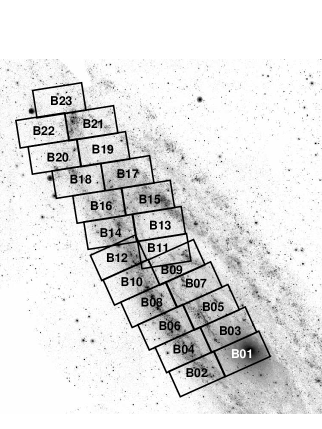
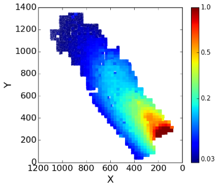
Figure 1.— Map of the portions of the PHAT survey for which we measured SFHs. Left: PHAT region from Williams et al. (2014) is shown on a GALEX NUV image of M31. Right Stellar density map of the PHAT region outlined in right. The areas measured are color-coded by stellar density for 18.5$<m_{F160W}<$19.5 (stars per arcsec²).

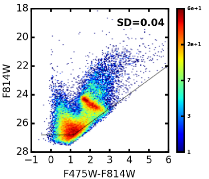
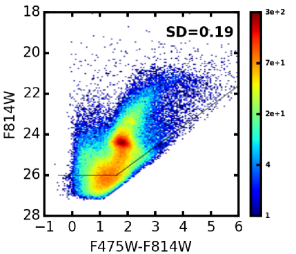
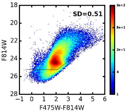
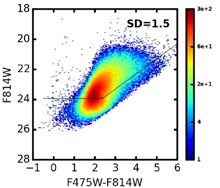
Figure 2.— Optical CMDs from 4 of our 83${}^{\prime\prime}{\times}83^{\prime\prime}$ regions covering the full range of stellar densities. Color indicates the number of data points in each place in the CMD. Black lines show the 50% completeness limits. Upper Left: Surface density (SD) = 0.04. Upper Right: SD=0.19. Lower Left: SD=0.51. Lower Right: SD=1.5.

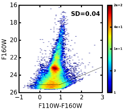
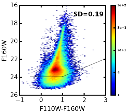
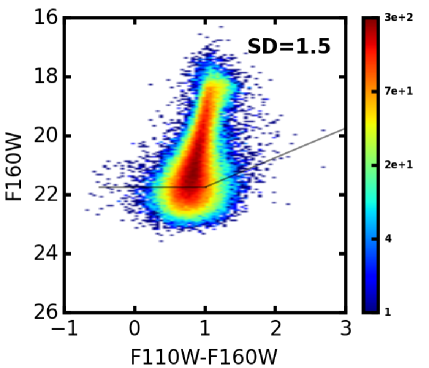
Figure 3.— Near IR CMDs from 4 of our regions covering the full range of stellar densities. Color indicates the number of data points in each place in the CMD. Black lines show the 50% completeness limits. Upper Left: 0.04. Upper Right: 0.19. Lower Left: 0.51. Lower Right: 1.5.

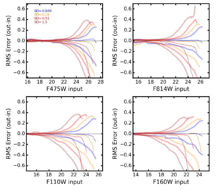
Figure 4.— Uncertainties as a function of magnitude at several stellar densities for the four bands used in our analysis of the PHAT photometry measured with the output magnitude minus the input magnitude from our artificial star tests. Color-coded broad lines mark the root-mean-square scatter in the positive and negative directions. Narrow lines mark the median difference (photometric bias). Redder lines denote higher stellar densities. Each panel shows the relation for a different band.

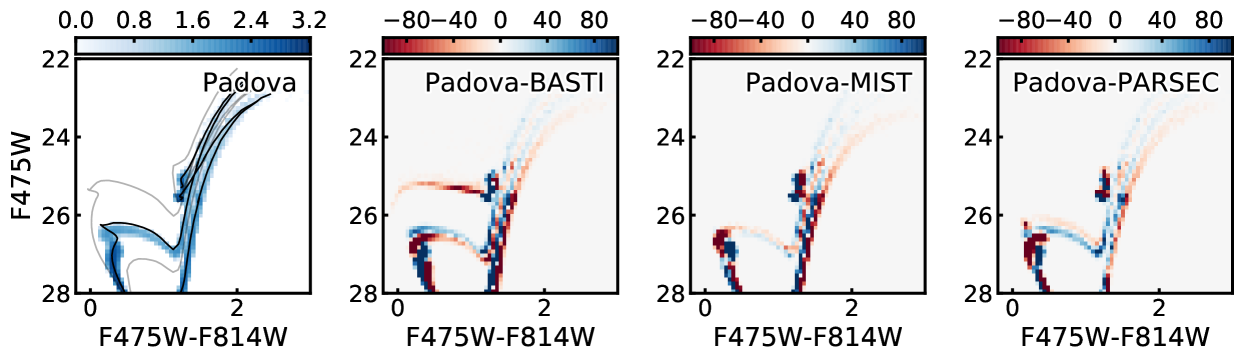
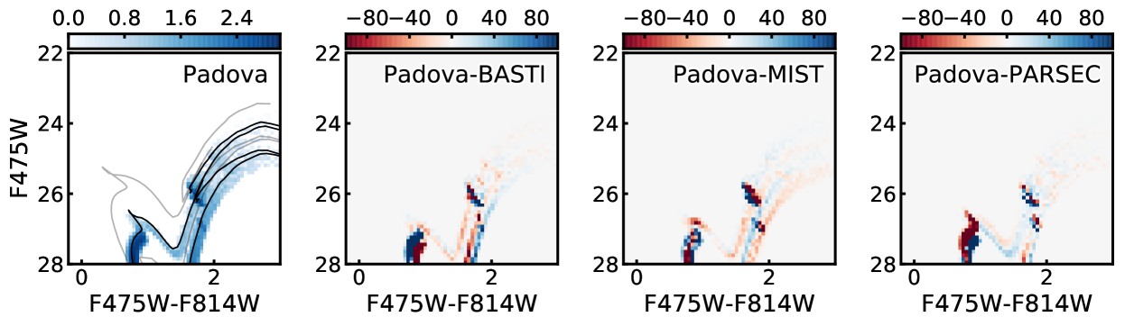
Figure 5.— Top: Left panel shows an example CMD of the Padova models at with ages of 2 and 10 Gyr at metallicity Z=0.0018. Dispersion is due to the use of finite age and metallicity ranges (0.05 dex) to generate the models. Black lines mark the corresponding isochrones for ages of 2 and 10 Gyr. Gray lines mark isochrones for 1 Gyr and 4 Gyr. Other panels show the differences between this CMD and those with the same ages and metallicity for the other three models sets used in our analysis. Bottom: Same as Top, but for Z=0.018.

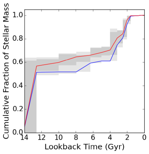
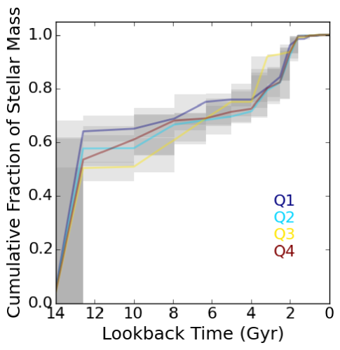
Figure 6.— Left: Cumulative SFH for a region as measured with ASTs performed directly on the data (blue) are overplotted with the SFH of for the same region as measured with ASTs calculated using our stellar density function fitting technique to infer the photometric quality as a function of color and magnitude at the stellar density of the region (red). Gray area shows the random uncertainties from the measurement, areas where the uncertainties overlap are darker gray. Right: Cumulative SFH for a region as measured by the samples taken from the 4 quartiles of A_V ($\mu$) values. Colors indicate the different quartiles. There is no trend with quartiles, and the measurements agree within their uncertainties.

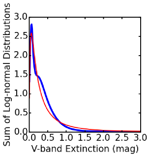
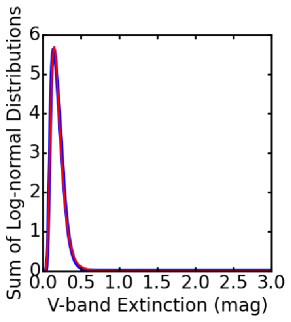
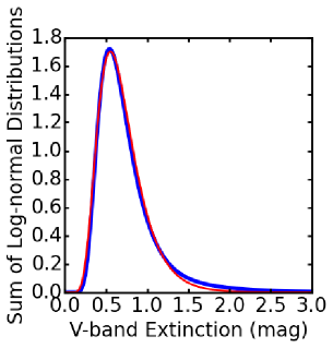
Figure 7.— Left: Log-normal fit to a sum of the log-normal functions of all of the pixels in the Dalcanton et al. (2015) maps of one of our sub-regions. Center Log-normal fit to a sum of the log-normal functions of pixels in the second quartile of $\mu$ values in Dalcanton et al. (2015) maps of one of our sub-regions ($\mu=0.18,\sigma=0.43$). Right Log-normal fit to a sum of the log-normal functions of pixels in the forth quartile of $\mu$ values in Dalcanton et al. (2015) maps of one of our sub-regions ($\mu=0.65,\sigma=0.39$).

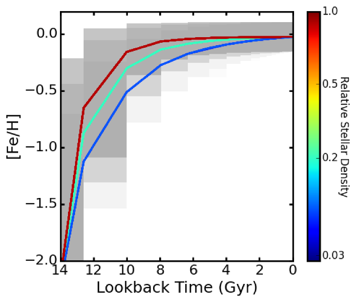
Figure 8.— Enrichment models adopted for three radial divisions, using the same color-coding as in Figure 1. Gray areas show the spread in metallicity allowed in each epoch. The inner regions enrich faster earlier, while the outer regions have more constant enrichment.

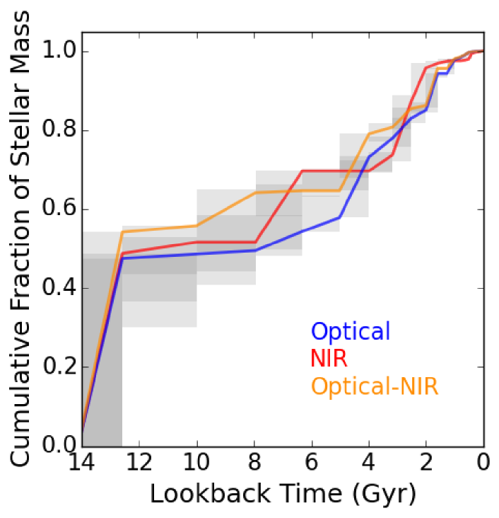
Figure 9.— Cumulative stellar mass with age measured for one of our regions by fitting the near-IR data only (red), the optical data only (blue), and simultaneously fitting both (orange). The gray shaded areas show the random uncertainties for each fit. Darker areas show where the uncertainties from the different fits overlap.

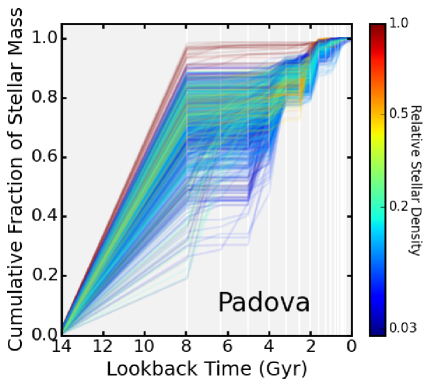
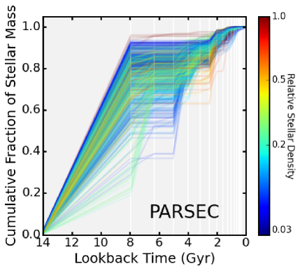
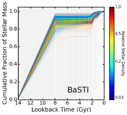
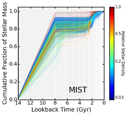
Figure 10.— Cumulative SFHs for the survey with different stellar evolution models for a forced enrichment scenario. Lines are color-coded by their values in Figure 1, and panels are labeled with their corresponding isochrones set.

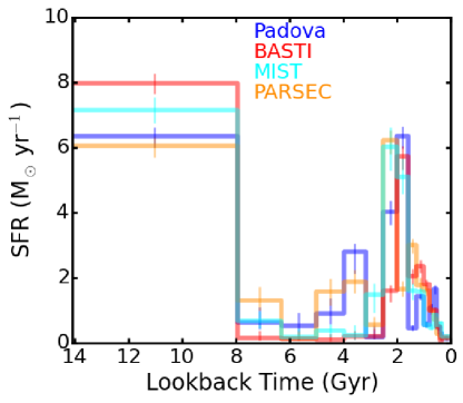
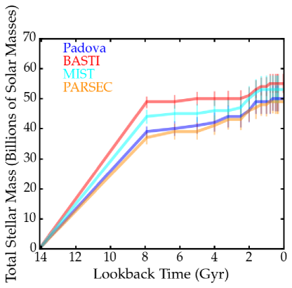
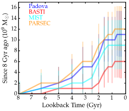
Figure 11.— Left: Total star formation rate vs. age for the entire PHAT footprint, as measured using 4 different model sets. Middle: The cumulative stellar mass formed as a function of time. Right: Same as Middle, but starting removing the oldest bin of star formation to more clearly compare the results at younger ages.

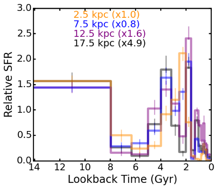
Figure 12.— Total relative star formation rate vs. age from the Padova model fits for 4 radial bins, color-coded by the radius used for the measurements, normalized to have the same mean rate of 1 M_⊙ yr^-1.

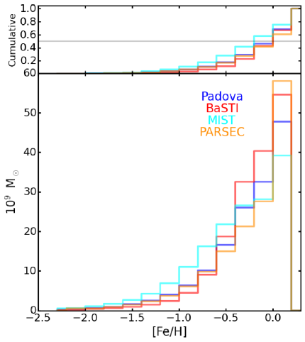
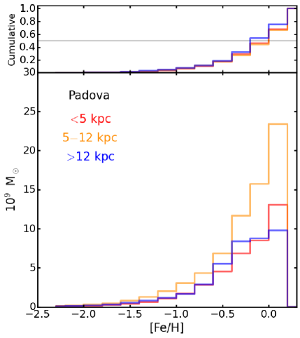
Figure 13.— Left: Metallicity histograms for the entire M31 disk when using our fixed enrichment model, extrapolated from the entire area measured. The cumulative fraction of stars as a function on metallicity is included in the top panel. The distribution for all 4 model sets is shown. Right: Metallicity histograms for 3 radial bins when using our fixed enrichment model and fitting with the Padova stellar evolution models, correcting for area coverage. The cumulative fraction of stars as a function on metallicity is included in the top panel.

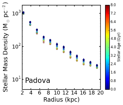
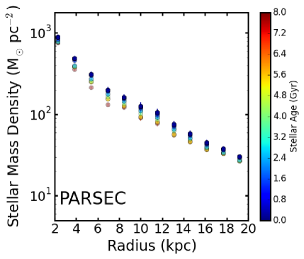
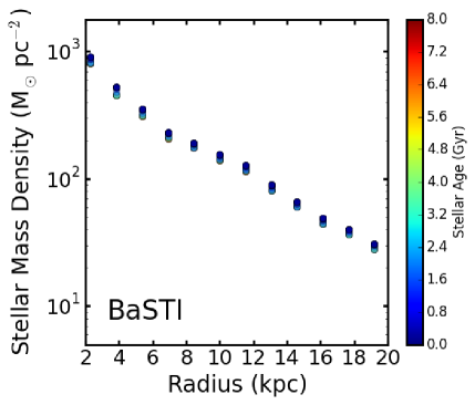
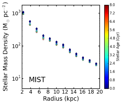
Figure 14.— Cumulative stellar mass surface density formed as a function of radius at several ages (lookback times), as calculated from the fits to 4 model sets. The error bars are the linear sum of the random uncertainties on the total star formation in each spatial bin in the annulus at each age. Upper-left The mass profile obtained for each age from the fits to the Padova models. Other panels: Same as upper-left from the other model fits. Each panel is labeled with the appropriate model set name.

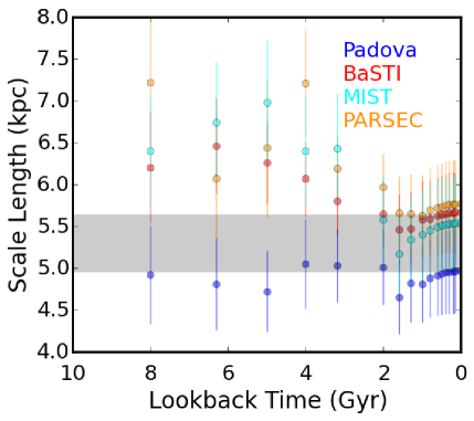
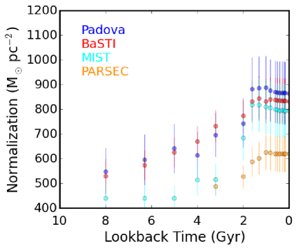
Figure 15.— Exponential fits to the disk profile of M31 beyond 4 kpc as a function of lookback time as calculated from our fits using the scipy function curve_fit. Left: Disk scale length as a function of lookback time. Right: Normalization of the exponential disk as a function of lookback time.

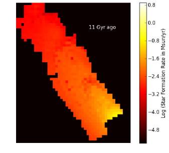
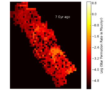
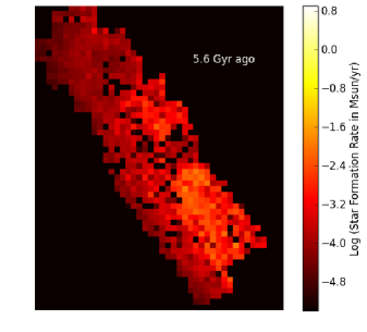
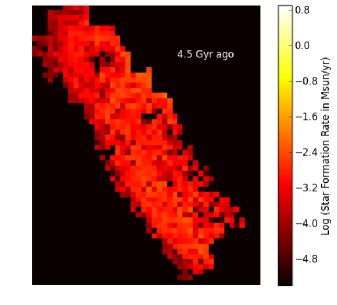
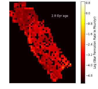
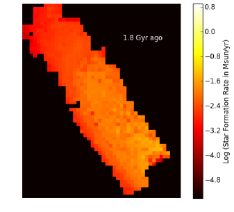
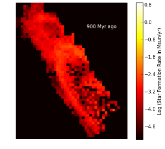
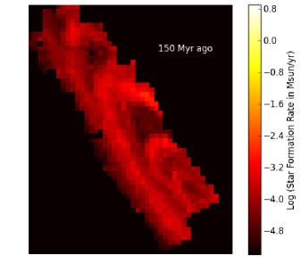
Figure 16.— Subsample of SFH maps from the star formation movie made from the Padova model fits to the PHAT survey.

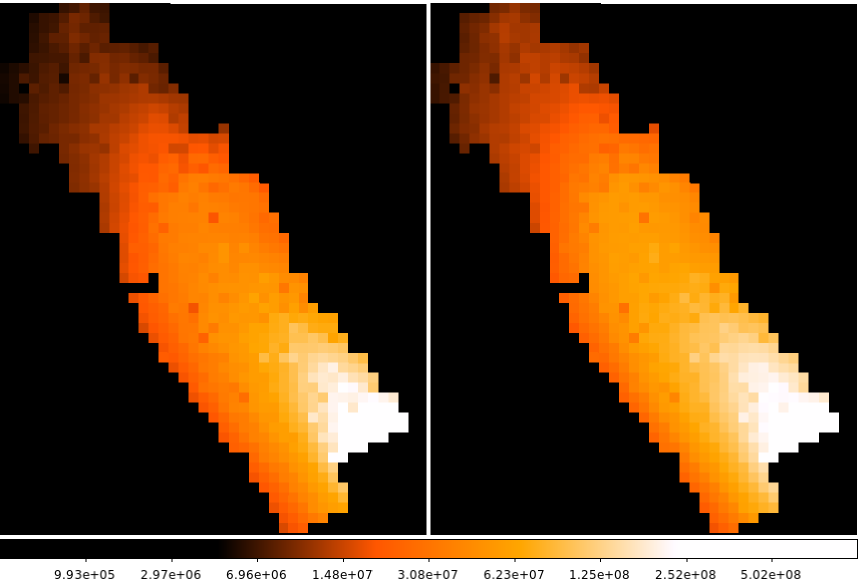
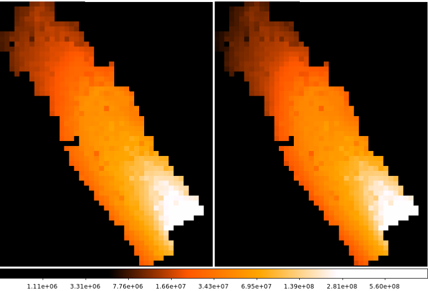
Figure 17.— Total stellar mass in each 83${}^{\prime\prime}{\times}83^{\prime\prime}$ region of the PHAT survey from the 4 different model sets. Upper Left: Padova fits. Upper Right: BaSTI fits. Lower Left: PARSEC fits. Lower Right: MIST fits.

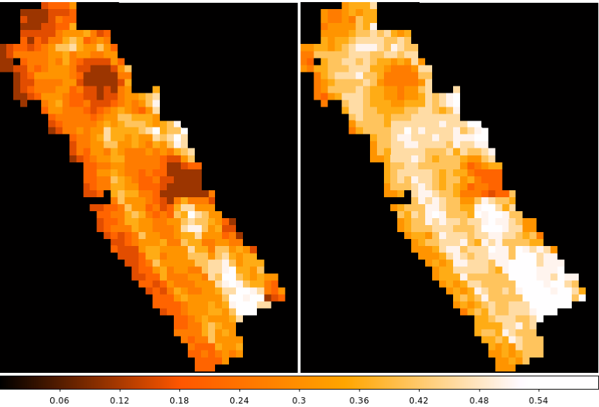
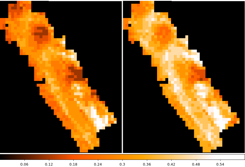
Figure 18.— Maps of the best-fitting foreground $A_{\rm VFG}$ values in each 83${}^{\prime\prime}{\times}83^{\prime\prime}$ region of the PHAT survey from the 4 different model sets. Upper Left: Padova fits. Upper Right: BaSTI fits. Lower Left: PARSEC fits. Lower Right: MIST fits.

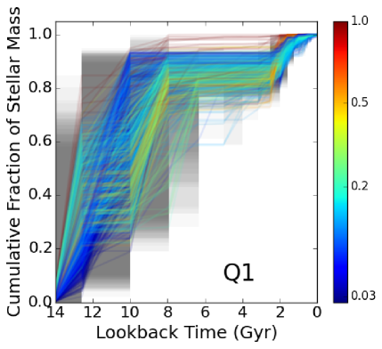
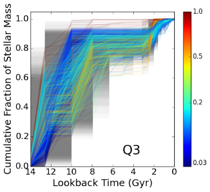
Figure 19.— Left: The SFHs measured for the first quartile of $\mu$ values in each region, color coded by stellar density using the same colors as Figure 1. Right: Same as center, but for the third quartile in all fields. These examples are from the MIST model fits.

5. Appendix: Metallicity as a Free Parameter

In this Appendix, we show the SFH results when fitting the data with the metallicity as a free parameter for each age. The resulting enrichment histories are shown in Figure 20. SFR in each metallicity and time are provided in Table 7; total rates and uncertainties for each time bin are provided in Table 8. Total rates and masses are given in Tables 9 and 10. In Figure 21, we show the SFH results when the metallicity is fitted as a free parameter at all ages. This figure is analogous to Figure 10. In Figure 22, we show the total SFH of the PHAT footprint. This figure is analogous to Figure 11. In Figure 23, we break the total into 4 radial bins, as in Figure 12. Figure 24 shows histograms of the resulting total metallicity distribution of the M31 disk for these SFHs, as well as the variations with radius in the Padova fits, comparable to Figure 13 in the main text. In Figure 25, we show the resulting build-up of the stellar mass in the disk analogous to Figure 14. In Figure 26, we show the exponential parameters of the stellar mass profile as a function of lookback time. The Padova and BaSTI results are shown; analogous to Figure 15. In Figure 27, we show maps of the stellar mass formed at a variety of ages, analogous to Figure 16 in the main text. Below, we compare these to the results with our adopted chemical enrichment model. Figure 28 shows the total stellar mass maps, analogous to Figure 17. Figure 29 shows a map of the best-fit foreground extinction values for these SFHs, analogous to Figure 18.

The largest systematic offset between models in the free metallicity fits is seen in the PARSEC models with the metallicity fitted as a free parameter. Those fits result in systematically lower stellar masses, and younger ages, at smaller radii, which is not consistent with previous work (e.g. Saglia et al., 2010; Dong et al., 2015). This difference is not apparent in the fits presented in the main text, suggesting that fixing the enrichment model was most important when applying this model set.

Another interesting feature is seen in the enrichment histories (Figures 20) is the dip in metallicity seen at 2-3 Gyr, which is clearest in the Padova fits, but also present in the other model fits. This dip in metallicity is coincident in age with the last global star formation episode. This episode is seen in all of the SFHs, regardless of the enrichment history, and it is clearly visible in the 1.8 Gyr panel of the SFR maps we provide in Figures 16 and 27. However, since the outburst appears with or without a forced enrichment history, the data appear relatively insensitive to the metallicity at this age. Thus, while it may appear that this feature of the free metallicity fits provides some tantalizing evidence that this powerful star forming episode may have been accompanied by the accretion of low metallicity gas, deeper data would be necessary to make such a claim. For now, we can only detect the large stellar mass present at this age range.

As a final note on the effects of fixing the enrichment history, in Figure 30 we show the NIR CMD of some dust-free regions of the PHAT survey (as measured by Dalcanton et al., 2015) overlaid with Padova isochrones. The narrow RGBs in the NIR show that there is a dominant metallicity, which is [Fe/H]${\sim}-$0.5. Because the adopted enrichment history only allows specific metallicities to be fitted at specific ages, the fits will necessarily increase the rates at ages where [Fe/H]${\sim}-$0.5. In our best-fitting enrichment model, presented in the main text, the metallicity reaches this range at $>$8 Gyr ago. Thus both fitting techniques agree that the bulk of the stellar mass was formed prior to 8 Gyr ago.

Table 7M31 Star Formation Rates by Metallicity (M_⊙ yr^-1) for the free metallicity fits; Columns are age range in Gyr; full table available in electronic format only

Model Set	RA	Dec	[Fe/H]	0.0-0.3	0.3-0.4	0.4-0.5	0.5-0.6	0.6-0.8	0.8-1.0	1.0-1.3	1.3-1.6	1.6-2.0	2.0-2.5	2.5-3.2	3.2-4.0	4.0-5.0	5.0-6.3	6.3-7.9	7.9-14.1
Padova	0:42:45.03	41:22:17.0	-2.25	2.4e-04	0.0e+00	0.0e+00	0.0e+00	0.0e+00	0.0e+00	0.0e+00	0.0e+00	0.0e+00	0.0e+00	0.0e+00	0.0e+00	0.0e+00	0.0e+00	1.1e-04	4.6e-03
Padova	0:42:45.03	41:22:17.0	-2.15	1.8e-04	0.0e+00	0.0e+00	0.0e+00	0.0e+00	0.0e+00	0.0e+00	0.0e+00	0.0e+00	0.0e+00	0.0e+00	0.0e+00	0.0e+00	0.0e+00	0.0e+00	0.0e+00
Padova	0:42:45.03	41:22:17.0	-2.05	1.6e-06	0.0e+00	0.0e+00	0.0e+00	0.0e+00	0.0e+00	0.0e+00	0.0e+00	0.0e+00	0.0e+00	0.0e+00	0.0e+00	0.0e+00	0.0e+00	0.0e+00	0.0e+00
Padova	0:42:45.03	41:22:17.0	-1.95	8.1e-05	0.0e+00	0.0e+00	0.0e+00	0.0e+00	0.0e+00	0.0e+00	0.0e+00	0.0e+00	0.0e+00	0.0e+00	0.0e+00	0.0e+00	0.0e+00	0.0e+00	0.0e+00
Padova	0:42:45.03	41:22:17.0	-1.85	4.3e-06	0.0e+00	0.0e+00	0.0e+00	0.0e+00	0.0e+00	0.0e+00	6.4e-04	0.0e+00	0.0e+00	0.0e+00	0.0e+00	0.0e+00	0.0e+00	0.0e+00	0.0e+00
Padova	0:42:45.03	41:22:17.0	-1.75	2.8e-05	0.0e+00	0.0e+00	0.0e+00	0.0e+00	0.0e+00	0.0e+00	0.0e+00	0.0e+00	0.0e+00	0.0e+00	0.0e+00	0.0e+00	0.0e+00	0.0e+00	0.0e+00
Padova	0:42:45.03	41:22:17.0	-1.65	8.2e-05	0.0e+00	0.0e+00	0.0e+00	0.0e+00	0.0e+00	0.0e+00	0.0e+00	0.0e+00	0.0e+00	0.0e+00	0.0e+00	0.0e+00	0.0e+00	0.0e+00	6.0e-05
Padova	0:42:45.03	41:22:17.0	-1.55	0.0e+00	0.0e+00	0.0e+00	0.0e+00	0.0e+00	0.0e+00	0.0e+00	0.0e+00	0.0e+00	0.0e+00	0.0e+00	0.0e+00	0.0e+00	0.0e+00	0.0e+00	0.0e+00
Padova	0:42:45.03	41:22:17.0	-1.45	1.7e-04	0.0e+00	0.0e+00	0.0e+00	0.0e+00	0.0e+00	0.0e+00	0.0e+00	0.0e+00	0.0e+00	0.0e+00	0.0e+00	0.0e+00	0.0e+00	0.0e+00	6.5e-05
Padova	0:42:45.03	41:22:17.0	-1.35	7.2e-05	1.3e-05	0.0e+00	0.0e+00	0.0e+00	0.0e+00	0.0e+00	0.0e+00	0.0e+00	0.0e+00	0.0e+00	0.0e+00	0.0e+00	0.0e+00	0.0e+00	7.6e-04
Padova	0:42:45.03	41:22:17.0	-1.25	6.3e-05	3.2e-06	0.0e+00	0.0e+00	0.0e+00	0.0e+00	0.0e+00	0.0e+00	0.0e+00	0.0e+00	0.0e+00	0.0e+00	0.0e+00	0.0e+00	0.0e+00	7.3e-04
Padova	0:42:45.03	41:22:17.0	-1.15	7.2e-05	0.0e+00	0.0e+00	0.0e+00	0.0e+00	0.0e+00	0.0e+00	0.0e+00	0.0e+00	0.0e+00	0.0e+00	0.0e+00	0.0e+00	0.0e+00	0.0e+00	0.0e+00
Padova	0:42:45.03	41:22:17.0	-1.05	0.0e+00	0.0e+00	0.0e+00	0.0e+00	4.0e-05	0.0e+00	0.0e+00	0.0e+00	0.0e+00	0.0e+00	0.0e+00	0.0e+00	0.0e+00	0.0e+00	0.0e+00	1.7e-04
Padova	0:42:45.03	41:22:17.0	-0.95	3.2e-06	0.0e+00	0.0e+00	0.0e+00	6.3e-04	0.0e+00	0.0e+00	0.0e+00	5.5e-03	0.0e+00	0.0e+00	0.0e+00	0.0e+00	0.0e+00	0.0e+00	4.7e-04
Padova	0:42:45.03	41:22:17.0	-0.85	0.0e+00	0.0e+00	0.0e+00	1.2e-03	0.0e+00	7.9e-05	0.0e+00	0.0e+00	9.2e-03	0.0e+00	0.0e+00	0.0e+00	0.0e+00	0.0e+00	0.0e+00	4.6e-04
Padova	0:42:45.03	41:22:17.0	-0.75	0.0e+00	4.4e-06	3.3e-03	2.8e-03	1.2e-03	4.7e-04	0.0e+00	0.0e+00	9.1e-05	1.8e-02	0.0e+00	0.0e+00	0.0e+00	0.0e+00	0.0e+00	0.0e+00
Padova	0:42:45.03	41:22:17.0	-0.65	1.2e-05	3.1e-03	1.1e-02	1.8e-03	0.0e+00	0.0e+00	0.0e+00	0.0e+00	0.0e+00	2.2e-02	0.0e+00	0.0e+00	0.0e+00	0.0e+00	0.0e+00	0.0e+00
Padova	0:42:45.03	41:22:17.0	-0.55	1.9e-06	0.0e+00	4.5e-03	0.0e+00	0.0e+00	0.0e+00	0.0e+00	0.0e+00	3.9e-04	0.0e+00	2.4e-02	0.0e+00	0.0e+00	0.0e+00	0.0e+00	0.0e+00
Padova	0:42:45.03	41:22:17.0	-0.45	8.0e-06	0.0e+00	0.0e+00	0.0e+00	0.0e+00	0.0e+00	0.0e+00	0.0e+00	9.8e-04	0.0e+00	4.3e-02	1.7e-03	0.0e+00	0.0e+00	1.5e-03	1.5e-03
Padova	0:42:45.03	41:22:17.0	-0.35	0.0e+00	0.0e+00	0.0e+00	0.0e+00	0.0e+00	0.0e+00	0.0e+00	0.0e+00	0.0e+00	0.0e+00	0.0e+00	0.0e+00	0.0e+00	0.0e+00	1.0e-04	1.1e-02
Padova	0:42:45.03	41:22:17.0	-0.25	7.2e-06	0.0e+00	3.7e-04	0.0e+00	0.0e+00	0.0e+00	0.0e+00	0.0e+00	3.2e-04	0.0e+00	0.0e+00	5.1e-04	0.0e+00	0.0e+00	0.0e+00	0.0e+00
Padova	0:42:45.03	41:22:17.0	-0.15	7.0e-06	0.0e+00	0.0e+00	0.0e+00	0.0e+00	0.0e+00	0.0e+00	0.0e+00	0.0e+00	0.0e+00	7.5e-04	0.0e+00	0.0e+00	0.0e+00	2.8e-04	0.0e+00
Padova	0:42:45.03	41:22:17.0	-0.05	4.6e-06	0.0e+00	0.0e+00	0.0e+00	0.0e+00	0.0e+00	0.0e+00	0.0e+00	0.0e+00	3.6e-04	0.0e+00	1.2e-03	0.0e+00	3.4e-04	3.5e-04	0.0e+00
Padova	0:42:45.03	41:22:17.0	0.05	0.0e+00	0.0e+00	0.0e+00	5.4e-04	0.0e+00	0.0e+00	0.0e+00	0.0e+00	3.8e-04	3.2e-04	1.1e-04	0.0e+00	0.0e+00	0.0e+00	4.1e-03	1.0e-02
Padova	0:42:45.08	41:20:53.9	-2.25	4.7e-06	0.0e+00	0.0e+00	0.0e+00	0.0e+00	0.0e+00	0.0e+00	0.0e+00	0.0e+00	0.0e+00	0.0e+00	0.0e+00	0.0e+00	0.0e+00	0.0e+00	8.4e-05

Table 8M31 Star Formation Rates (10^-4 M_⊙ yr^-1 arcmin^-2 for free metallicity fits; Columns are age range in Gyr; full table available in electronic format only)

Model Set	RA	Dec	0.0-0.3	0.3-0.4	0.4-0.5	0.5-0.6	0.6-0.8	0.8-1.0	1.0-1.3	1.3-1.6	1.6-2.0	2.0-2.5	2.5-3.2	3.2-4.0	4.0-5.0	5.0-6.3	6.3-7.9	7.9-14.1
Padova	0:43:36.26	41:25:06.2	0.5${}^{+0.6}_{-0.5}$	0.6${}^{+0.3}_{-0.6}$	2.8${}^{+0.0}_{-2.4}$	17.6${}^{+3.5}_{-1.5}$	0.2${}^{+1.5}_{-0.2}$	1.2${}^{+0.6}_{-1.2}$	2.6${}^{+0.3}_{-2.4}$	3.8${}^{+0.0}_{-3.3}$	86.9${}^{+20.6}_{-8.3}$	273.1${}^{+8.2}_{-22.7}$	82.4${}^{+17.7}_{-2.5}$	115.8${}^{+32.5}_{-16.4}$	26.1${}^{+35.9}_{-13.8}$	5.6${}^{+1.9}_{-5.6}$	59.2${}^{+16.5}_{-6.3}$	102.2${}^{+4.6}_{-9.9}$
Padova	0:43:36.29	41:23:43.2	0.9${}^{+0.9}_{-0.8}$	0.6${}^{+0.7}_{-0.5}$	6.3${}^{+0.0}_{-5.0}$	17.9${}^{+9.7}_{-1.2}$	8.8${}^{+6.1}_{-4.9}$	1.7${}^{+1.5}_{-1.7}$	4.9${}^{+3.4}_{-3.7}$	5.5${}^{+2.0}_{-4.7}$	66.5${}^{+27.9}_{-0.0}$	319.5${}^{+1.9}_{-35.5}$	97.0${}^{+22.5}_{-0.2}$	158.0${}^{+4.7}_{-20.8}$	2.4${}^{+6.8}_{-2.0}$	28.6${}^{+6.7}_{-9.1}$	56.3${}^{+15.4}_{-3.4}$	79.1${}^{+5.5}_{-7.6}$
Padova	0:43:36.32	41:22:20.1	2.2${}^{+1.6}_{-1.6}$	0.6${}^{+0.7}_{-0.4}$	6.3${}^{+0.0}_{-3.9}$	21.1${}^{+5.9}_{-0.0}$	3.5${}^{+2.7}_{-2.2}$	0.8${}^{+0.8}_{-0.8}$	3.1${}^{+0.8}_{-2.2}$	5.7${}^{+0.7}_{-3.4}$	88.6${}^{+19.0}_{-2.5}$	263.0${}^{+7.5}_{-19.5}$	73.7${}^{+18.4}_{-3.3}$	137.2${}^{+15.2}_{-19.0}$	35.6${}^{+21.3}_{-10.3}$	27.0${}^{+7.7}_{-16.4}$	65.1${}^{+22.1}_{-1.6}$	74.9${}^{+4.0}_{-9.6}$
Padova	0:43:36.36	41:20:57.0	1.5${}^{+1.0}_{-1.1}$	0.8${}^{+0.8}_{-0.6}$	7.0${}^{+1.5}_{-3.8}$	29.0${}^{+6.1}_{-3.3}$	5.0${}^{+2.4}_{-2.7}$	0.0${}^{+1.2}_{-0.0}$	1.0${}^{+0.6}_{-0.9}$	4.6${}^{+1.1}_{-2.6}$	128.4${}^{+22.5}_{-0.0}$	159.4${}^{+12.8}_{-13.5}$	207.8${}^{+16.1}_{-4.1}$	53.7${}^{+0.0}_{-24.1}$	8.6${}^{+8.6}_{-2.7}$	7.0${}^{+7.8}_{-5.0}$	88.3${}^{+15.3}_{-3.8}$	88.1${}^{+9.8}_{-9.2}$
Padova	0:43:36.39	41:19:34.0	1.0${}^{+0.7}_{-0.7}$	1.2${}^{+0.7}_{-0.8}$	6.0${}^{+0.0}_{-3.7}$	21.3${}^{+5.6}_{-0.0}$	3.0${}^{+1.5}_{-1.5}$	1.0${}^{+3.0}_{-0.4}$	2.5${}^{+2.0}_{-1.4}$	2.4${}^{+0.0}_{-2.2}$	79.8${}^{+18.6}_{-1.3}$	231.1${}^{+0.0}_{-21.4}$	63.9${}^{+18.6}_{-0.0}$	91.4${}^{+7.9}_{-16.0}$	26.1${}^{+11.1}_{-0.2}$	58.1${}^{+3.7}_{-13.3}$	27.8${}^{+10.3}_{-6.8}$	83.0${}^{+5.8}_{-7.2}$
Padova	0:43:36.42	41:18:10.9	0.4${}^{+0.4}_{-0.2}$	2.8${}^{+0.0}_{-2.0}$	5.8${}^{+0.6}_{-2.5}$	14.3${}^{+4.6}_{-0.0}$	2.5${}^{+0.8}_{-1.3}$	0.1${}^{+1.1}_{-0.0}$	2.6${}^{+0.0}_{-1.5}$	2.0${}^{+0.0}_{-1.5}$	124.9${}^{+7.1}_{-5.8}$	201.3${}^{+11.5}_{-1.5}$	39.3${}^{+8.3}_{-1.7}$	60.3${}^{+0.6}_{-15.9}$	23.5${}^{+11.9}_{-1.3}$	38.7${}^{+5.2}_{-6.3}$	18.8${}^{+2.4}_{-9.5}$	83.8${}^{+7.0}_{-6.0}$
Padova	0:43:36.45	41:16:47.8	0.9${}^{+1.1}_{-0.5}$	7.1${}^{+0.0}_{-5.9}$	5.3${}^{+8.1}_{-0.1}$	38.3${}^{+5.6}_{-4.5}$	5.3${}^{+1.6}_{-2.8}$	2.8${}^{+8.2}_{-0.8}$	89.0${}^{+0.1}_{-11.7}$	2.2${}^{+0.1}_{-1.7}$	68.6${}^{+10.7}_{-1.7}$	165.5${}^{+10.1}_{-6.5}$	58.8${}^{+10.1}_{-10.6}$	123.2${}^{+0.2}_{-23.5}$	32.5${}^{+25.4}_{-0.2}$	129.6${}^{+15.7}_{-10.0}$	24.9${}^{+6.0}_{-11.8}$	98.4${}^{+7.9}_{-4.6}$
Padova	0:43:36.48	41:15:24.8	0.5${}^{+0.4}_{-0.3}$	2.8${}^{+0.0}_{-1.7}$	4.1${}^{+0.3}_{-1.8}$	13.9${}^{+4.2}_{-0.0}$	8.8${}^{+0.0}_{-3.4}$	3.2${}^{+2.2}_{-0.6}$	3.5${}^{+0.0}_{-2.2}$	3.3${}^{+0.0}_{-2.1}$	107.9${}^{+14.5}_{-0.0}$	56.4${}^{+0.1}_{-7.8}$	14.2${}^{+0.5}_{-6.1}$	24.9${}^{+5.3}_{-4.5}$	34.2${}^{+6.0}_{-3.2}$	26.9${}^{+4.5}_{-5.8}$	31.2${}^{+0.3}_{-9.1}$	68.3${}^{+5.1}_{-2.3}$
Padova	0:43:36.51	41:14:01.7	0.7${}^{+0.5}_{-0.3}$	3.0${}^{+0.0}_{-2.4}$	8.1${}^{+1.4}_{-1.1}$	17.0${}^{+3.2}_{-0.0}$	1.0${}^{+0.5}_{-0.6}$	3.3${}^{+1.5}_{-0.6}$	28.2${}^{+2.0}_{-0.8}$	0.3${}^{+0.2}_{-0.2}$	33.9${}^{+4.2}_{-3.6}$	52.0${}^{+1.1}_{-5.8}$	39.5${}^{+2.5}_{-1.9}$	35.2${}^{+7.2}_{-2.5}$	23.9${}^{+4.4}_{-5.4}$	13.0${}^{+4.6}_{-4.0}$	14.2${}^{+1.2}_{-4.1}$	60.8${}^{+3.5}_{-2.0}$
Padova	0:43:36.54	41:12:38.7	0.8${}^{+0.7}_{-0.3}$	4.9${}^{+0.0}_{-3.1}$	5.8${}^{+1.6}_{-1.1}$	19.8${}^{+3.9}_{-0.0}$	7.8${}^{+0.0}_{-2.4}$	3.0${}^{+2.0}_{-0.0}$	19.9${}^{+1.4}_{-0.0}$	1.0${}^{+0.0}_{-0.8}$	6.5${}^{+0.0}_{-4.0}$	14.9${}^{+0.1}_{-6.5}$	29.4${}^{+3.6}_{-1.9}$	51.6${}^{+4.0}_{-1.9}$	44.4${}^{+8.3}_{-0.0}$	12.7${}^{+1.5}_{-4.8}$	10.4${}^{+1.9}_{-3.4}$	45.3${}^{+2.3}_{-2.3}$
Padova	0:43:36.57	41:11:15.6	0.9${}^{+0.5}_{-0.5}$	6.8${}^{+0.4}_{-1.3}$	3.6${}^{+0.6}_{-1.0}$	20.5${}^{+1.9}_{-0.0}$	0.8${}^{+0.0}_{-0.7}$	7.1${}^{+1.7}_{-0.0}$	21.9${}^{+1.1}_{-0.6}$	0.8${}^{+0.0}_{-0.6}$	47.5${}^{+4.6}_{-0.7}$	10.5${}^{+0.0}_{-3.3}$	38.0${}^{+3.9}_{-1.0}$	12.6${}^{+0.0}_{-4.1}$	11.1${}^{+0.8}_{-3.8}$	6.4${}^{+7.0}_{-0.0}$	4.0${}^{+0.9}_{-2.7}$	39.9${}^{+2.0}_{-2.3}$
Padova	0:43:36.60	41:09:52.5	1.4${}^{+0.7}_{-0.3}$	1.6${}^{+0.0}_{-1.0}$	4.4${}^{+0.4}_{-1.0}$	12.0${}^{+1.9}_{-0.0}$	0.7${}^{+0.0}_{-0.6}$	4.9${}^{+0.4}_{-0.6}$	16.9${}^{+1.6}_{-0.0}$	2.0${}^{+0.0}_{-1.5}$	47.4${}^{+3.8}_{-0.0}$	4.4${}^{+0.0}_{-3.1}$	20.5${}^{+3.8}_{-0.0}$	23.5${}^{+0.0}_{-5.5}$	2.2${}^{+2.5}_{-0.3}$	6.3${}^{+3.2}_{-0.1}$	2.6${}^{+0.1}_{-2.2}$	38.4${}^{+1.9}_{-1.5}$
Padova	0:43:43.37	41:36:11.1	0.7${}^{+0.7}_{-0.4}$	6.3${}^{+0.0}_{-2.6}$	2.5${}^{+0.4}_{-0.9}$	6.8${}^{+3.6}_{-0.0}$	10.4${}^{+0.2}_{-2.5}$	2.3${}^{+0.0}_{-1.8}$	18.5${}^{+3.8}_{-0.0}$	0.0${}^{+0.2}_{-0.0}$	59.7${}^{+1.3}_{-3.4}$	1.9${}^{+0.0}_{-1.4}$	18.3${}^{+2.4}_{-0.9}$	83.6${}^{+9.5}_{-0.1}$	15.2${}^{+0.1}_{-5.4}$	0.0${}^{+0.6}_{-0.0}$	1.9${}^{+0.0}_{-1.6}$	36.2${}^{+2.2}_{-2.3}$

Table 9Total Star Formation Rates

Lookback Start (Years)	Lookback End (Years)	Padova SFR (M⊙ yr-1)	$+$error	$-$error	BaSTI SFR	$+$error	$-$error	PARSEC SFR	$+$error	$-$error	MIST SFR	$+$error	$-$error
3.2e+08	4.0e+06	1.5e-01	6.3e-02	8.1e-02	2.1e-01	3.2e-02	2.9e-02	1.6e-01	7.1e-02	8.5e-02	2.1e-01	8.3e-02	8.0e-02
4.0e+08	3.2e+08	4.2e-01	7.0e-02	1.7e-01	2.1e-01	2.7e-02	3.1e-02	1.6e-01	4.8e-02	7.9e-02	5.3e-01	1.1e-01	1.8e-01
5.0e+08	4.0e+08	7.5e-01	1.3e-01	2.1e-01	6.1e-01	5.6e-02	5.7e-02	3.9e-01	6.1e-02	1.5e-01	7.5e-01	1.9e-01	1.4e-01
6.3e+08	5.0e+08	1.3e+00	3.4e-01	8.9e-02	9.6e-01	8.3e-02	7.7e-02	1.1e+00	2.5e-01	1.2e-01	5.0e-01	1.8e-01	6.9e-02
7.9e+08	6.3e+08	6.7e-01	1.1e-01	1.8e-01	3.4e-01	8.9e-02	4.7e-02	8.5e-01	2.2e-01	1.4e-01	2.7e-01	5.7e-02	8.6e-02
1.0e+09	7.9e+08	7.8e-01	1.4e-01	9.8e-02	1.3e+00	1.0e-01	8.5e-02	6.5e-01	1.2e-01	2.0e-01	7.3e-01	9.7e-02	9.0e-02
1.3e+09	1.0e+09	1.4e+00	1.2e-01	1.3e-01	2.7e+00	2.3e-01	1.2e-01	2.3e+00	2.7e-01	2.7e-01	1.9e+00	2.4e-01	1.4e-01
1.6e+09	1.3e+09	2.4e-01	4.0e-02	1.1e-01	2.4e+00	1.6e-01	1.9e-01	5.4e+00	4.5e-01	1.9e-01	1.1e+00	1.5e-01	2.4e-01
2.0e+09	1.6e+09	5.3e+00	5.5e-01	2.3e-01	2.7e+00	2.9e-01	1.9e-01	2.3e+00	2.7e-01	3.0e-01	4.6e+00	6.1e-01	2.5e-01
2.5e+09	2.0e+09	4.4e+00	2.7e-01	4.8e-01	2.6e+00	2.2e-01	1.8e-01	3.5e+00	3.5e-01	3.7e-01	6.2e+00	4.5e-01	5.0e-01
3.2e+09	2.5e+09	3.5e+00	4.7e-01	3.0e-01	1.2e+00	1.5e-01	1.6e-01	2.2e+00	2.5e-01	4.3e-01	5.9e+00	5.4e-01	4.5e-01
4.0e+09	3.2e+09	4.4e+00	6.2e-01	4.3e-01	1.2e+00	1.3e-01	1.5e-01	4.5e+00	5.6e-01	3.3e-01	5.9e-01	2.3e-01	2.4e-01
5.0e+09	4.0e+09	1.9e+00	4.3e-01	2.9e-01	9.7e-01	1.4e-01	1.7e-01	3.8e+00	6.1e-01	2.8e-01	1.7e+00	3.1e-01	3.4e-01
6.3e+09	5.0e+09	8.1e-01	2.0e-01	2.9e-01	1.2e+00	1.4e-01	2.1e-01	1.6e+00	2.7e-01	2.4e-01	1.0e+00	2.7e-01	3.1e-01
7.9e+09	6.3e+09	1.2e+00	3.1e-01	3.0e-01	2.4e+00	2.5e-01	1.9e-01	2.7e+00	3.4e-01	4.7e-01	1.1e+00	2.2e-01	3.1e-01
1.4e+10	7.9e+09	5.2e+00	4.0e-01	3.6e-01	6.6e+00	3.8e-01	3.0e-01	3.3e+00	3.0e-01	2.7e-01	5.8e+00	4.2e-01	3.2e-01

Table 10Total Cumulative Mass

Lookback Time (Years)	Padova Mass (M⊙)	$+$error	$-$error	BaSTI Mass (M⊙)	$+$error	$-$error	PARSEC Mass (M⊙)	$+$error	$-$error	MIST Mass (M⊙)	$+$error	$-$error
7.9e+09	3.2e+10	2.5e+09	2.2e+09	4.1e+10	2.3e+09	1.8e+09	2.0e+10	1.9e+09	1.7e+09	3.6e+10	2.6e+09	2.0e+09
6.3e+09	3.4e+10	3.0e+09	2.7e+09	4.4e+10	2.7e+09	2.1e+09	2.5e+10	2.4e+09	2.4e+09	3.8e+10	3.0e+09	2.5e+09
5.0e+09	3.5e+10	3.2e+09	3.1e+09	4.6e+10	2.9e+09	2.4e+09	2.7e+10	2.8e+09	2.7e+09	3.9e+10	3.3e+09	2.9e+09
4.0e+09	3.7e+10	3.7e+09	3.4e+09	4.7e+10	3.1e+09	2.6e+09	3.1e+10	3.4e+09	3.0e+09	4.1e+10	3.7e+09	3.2e+09
3.2e+09	4.1e+10	4.2e+09	3.8e+09	4.8e+10	3.2e+09	2.7e+09	3.4e+10	3.8e+09	3.3e+09	4.1e+10	3.8e+09	3.4e+09
2.5e+09	4.3e+10	4.5e+09	4.0e+09	4.9e+10	3.3e+09	2.8e+09	3.6e+10	4.0e+09	3.6e+09	4.5e+10	4.2e+09	3.7e+09
2.0e+09	4.5e+10	4.6e+09	4.2e+09	5.0e+10	3.4e+09	2.9e+09	3.7e+10	4.2e+09	3.8e+09	4.8e+10	4.4e+09	4.0e+09
1.6e+09	4.7e+10	4.8e+09	4.3e+09	5.1e+10	3.5e+09	3.0e+09	3.8e+10	4.3e+09	3.9e+09	5.0e+10	4.7e+09	4.1e+09
1.3e+09	4.7e+10	4.9e+09	4.3e+09	5.2e+10	3.6e+09	3.0e+09	4.0e+10	4.4e+09	3.9e+09	5.1e+10	4.7e+09	4.2e+09
1.0e+09	4.8e+10	4.9e+09	4.4e+09	5.3e+10	3.6e+09	3.1e+09	4.1e+10	4.5e+09	4.0e+09	5.1e+10	4.8e+09	4.2e+09
7.9e+08	4.8e+10	4.9e+09	4.4e+09	5.3e+10	3.6e+09	3.1e+09	4.1e+10	4.5e+09	4.1e+09	5.1e+10	4.8e+09	4.2e+09
6.3e+08	4.8e+10	4.9e+09	4.4e+09	5.3e+10	3.6e+09	3.1e+09	4.1e+10	4.6e+09	4.1e+09	5.1e+10	4.8e+09	4.2e+09
5.0e+08	4.8e+10	5.0e+09	4.4e+09	5.3e+10	3.7e+09	3.1e+09	4.1e+10	4.6e+09	4.1e+09	5.1e+10	4.8e+09	4.2e+09
4.0e+08	4.8e+10	5.0e+09	4.5e+09	5.3e+10	3.7e+09	3.1e+09	4.1e+10	4.6e+09	4.1e+09	5.2e+10	4.9e+09	4.2e+09
3.2e+08	4.8e+10	5.0e+09	4.5e+09	5.3e+10	3.7e+09	3.1e+09	4.1e+10	4.6e+09	4.1e+09	5.2e+10	4.9e+09	4.3e+09
4.0e+06	4.8e+10	5.0e+09	4.5e+09	5.3e+10	3.7e+09	3.1e+09	4.1e+10	4.6e+09	4.2e+09	5.2e+10	4.9e+09	4.3e+09

Table 11Metallicity Distribution for the M31 Disk (Free Metallicity Fits).

[Fe/H]low	[Fe/H]high	Padova Mass (M⊙)	Padova Scaled (M⊙)	BaSTI Mass (M⊙)	BaSTI Scaled (M⊙)	PARSEC Mass (M⊙)	PARSEC Scaled (M⊙)	MIST Mass (M⊙)	MIST Scaled (M⊙)
-2.4	-2.2	6.0e+08	1.8e+09	6.0e+08	1.8e+09	-0.0e+00	-0.0e+00	1.1e+09	3.3e+09
-2.2	-2.0	3.3e+08	1.0e+09	9.1e+07	2.7e+08	7.3e+08	2.2e+09	1.0e+09	3.1e+09
-2.0	-1.8	3.8e+08	1.1e+09	2.3e+08	6.9e+08	4.5e+08	1.3e+09	1.2e+09	3.6e+09
-1.8	-1.6	2.7e+08	8.0e+08	2.2e+08	6.6e+08	1.6e+08	4.8e+08	5.8e+08	1.7e+09
-1.6	-1.4	4.9e+08	1.5e+09	2.2e+08	6.7e+08	2.9e+08	8.7e+08	7.6e+08	2.3e+09
-1.4	-1.2	2.4e+08	7.3e+08	3.4e+08	1.0e+09	7.0e+08	2.1e+09	1.0e+09	3.0e+09
-1.2	-1.0	6.0e+08	1.8e+09	8.0e+08	2.4e+09	7.5e+08	2.2e+09	1.8e+09	5.3e+09
-1.0	-0.8	1.5e+09	4.4e+09	1.6e+09	4.8e+09	1.4e+09	4.1e+09	4.2e+09	1.3e+10
-0.8	-0.6	2.5e+09	7.6e+09	4.5e+09	1.3e+10	2.3e+09	6.9e+09	2.9e+09	8.7e+09
-0.6	-0.4	7.7e+09	2.3e+10	6.9e+09	2.1e+10	4.8e+09	1.4e+10	7.0e+09	2.1e+10
-0.4	-0.2	8.4e+09	2.5e+10	1.0e+10	3.0e+10	7.9e+09	2.4e+10	8.3e+09	2.5e+10
-0.2	0.0	7.1e+09	2.1e+10	7.8e+09	2.3e+10	5.5e+09	1.7e+10	7.0e+09	2.1e+10
0.0	0.2	1.8e+10	5.5e+10	2.0e+10	6.0e+10	1.6e+10	4.9e+10	1.5e+10	4.4e+10

Table 12Metallicity Distribution in Radial Bins (Free Metallicity Fits).

Radial Range (kpc)	[Fe/H]low	[Fe/H]high	Padova Mass (M⊙)	Padova Scaled (M⊙)	BaSTI Mass (M⊙)	BaSTI Scaled (M⊙)	PARSEC Mass (M⊙)	PARSEC Scaled (M⊙)	MIST Mass (M⊙)	MIST Scaled (M⊙)
$<$5	-2.4	-2.2	2.4e+08	3.8e+08	1.5e+08	2.3e+08	-0.0e+00	-0.0e+00	1.6e+08	2.5e+08
$<$5	-2.2	-2.0	6.7e+07	1.1e+08	1.9e+07	3.1e+07	2.3e+08	4.8e+08	7.4e+08	1.2e+09
$<$5	-2.0	-1.8	1.2e+08	1.9e+08	3.6e+07	5.7e+07	1.2e+08	2.6e+08	4.4e+08	6.8e+08
$<$5	-1.8	-1.6	7.8e+07	1.2e+08	1.1e+08	1.8e+08	2.7e+07	5.6e+07	3.4e+08	5.3e+08
$<$5	-1.6	-1.4	7.9e+07	1.3e+08	3.9e+07	6.2e+07	7.3e+07	1.5e+08	3.6e+08	5.5e+08
$<$5	-1.4	-1.2	1.2e+08	1.9e+08	1.6e+08	2.6e+08	2.3e+08	4.9e+08	6.8e+08	1.1e+09
$<$5	-1.2	-1.0	2.8e+08	4.4e+08	2.8e+08	4.5e+08	2.5e+08	5.2e+08	9.0e+08	1.4e+09
$<$5	-1.0	-0.8	9.4e+08	1.5e+09	5.9e+08	9.4e+08	5.8e+08	1.2e+09	2.5e+09	3.8e+09
$<$5	-0.8	-0.6	2.0e+09	3.1e+09	2.9e+09	4.6e+09	1.1e+09	2.4e+09	9.1e+08	1.4e+09
$<$5	-0.6	-0.4	4.2e+09	6.7e+09	2.9e+09	4.6e+09	2.1e+09	4.4e+09	2.4e+09	3.7e+09
$<$5	-0.4	-0.2	3.5e+09	5.5e+09	3.5e+09	5.5e+09	2.4e+09	5.2e+09	3.2e+09	4.9e+09
$<$5	-0.2	0.0	2.8e+09	4.5e+09	2.8e+09	4.4e+09	2.4e+09	5.1e+09	3.7e+09	5.7e+09
$<$5	0.0	0.2	1.1e+10	1.7e+10	1.2e+10	1.9e+10	9.3e+09	2.0e+10	9.6e+09	1.5e+10
5$-$12	-2.4	-2.2	2.4e+08	9.8e+08	2.4e+08	7.9e+08	-0.0e+00	-0.0e+00	6.3e+08	2.3e+09
5$-$12	-2.2	-2.0	2.0e+08	8.0e+08	4.6e+07	1.5e+08	2.5e+08	1.1e+09	2.4e+08	8.9e+08
5$-$12	-2.0	-1.8	2.2e+08	8.9e+08	9.0e+07	3.0e+08	2.6e+08	1.1e+09	6.3e+08	2.3e+09
5$-$12	-1.8	-1.6	1.5e+08	6.0e+08	8.2e+07	2.7e+08	9.8e+07	4.2e+08	1.9e+08	7.0e+08
5$-$12	-1.6	-1.4	3.3e+08	1.3e+09	1.1e+08	3.7e+08	1.7e+08	7.3e+08	3.2e+08	1.2e+09
5$-$12	-1.4	-1.2	1.0e+08	4.2e+08	1.2e+08	4.1e+08	3.9e+08	1.7e+09	2.2e+08	8.1e+08
5$-$12	-1.2	-1.0	2.6e+08	1.1e+09	3.4e+08	1.1e+09	3.8e+08	1.6e+09	6.4e+08	2.3e+09
5$-$12	-1.0	-0.8	3.4e+08	1.4e+09	7.1e+08	2.4e+09	6.3e+08	2.7e+09	1.4e+09	4.9e+09
5$-$12	-0.8	-0.6	4.3e+08	1.8e+09	1.2e+09	4.0e+09	8.2e+08	3.5e+09	1.2e+09	4.2e+09
5$-$12	-0.6	-0.4	2.5e+09	1.0e+10	2.7e+09	8.9e+09	1.7e+09	7.2e+09	3.0e+09	1.1e+10
5$-$12	-0.4	-0.2	3.3e+09	1.3e+10	4.8e+09	1.6e+10	3.4e+09	1.5e+10	3.9e+09	1.4e+10
5$-$12	-0.2	0.0	2.8e+09	1.1e+10	3.6e+09	1.2e+10	2.2e+09	9.4e+09	2.8e+09	1.0e+10
5$-$12	0.0	0.2	6.4e+09	2.6e+10	7.0e+09	2.3e+10	6.0e+09	2.6e+10	4.3e+09	1.6e+10
$>$12	-2.4	-2.2	1.2e+08	8.2e+08	2.2e+08	1.2e+09	-0.0e+00	-0.0e+00	3.2e+08	1.9e+09
$>$12	-2.2	-2.0	7.0e+07	4.8e+08	2.6e+07	1.5e+08	2.5e+08	1.6e+09	5.1e+07	3.1e+08
$>$12	-2.0	-1.8	4.4e+07	3.0e+08	1.0e+08	5.8e+08	5.8e+07	3.7e+08	1.5e+08	9.1e+08
$>$12	-1.8	-1.6	4.0e+07	2.7e+08	2.5e+07	1.4e+08	3.5e+07	2.3e+08	4.7e+07	2.9e+08
$>$12	-1.6	-1.4	7.6e+07	5.2e+08	7.3e+07	4.1e+08	4.9e+07	3.2e+08	8.0e+07	4.8e+08
$>$12	-1.4	-1.2	2.1e+07	1.5e+08	5.7e+07	3.2e+08	8.6e+07	5.5e+08	1.0e+08	6.2e+08
$>$12	-1.2	-1.0	6.4e+07	4.4e+08	1.8e+08	1.0e+09	1.2e+08	7.9e+08	2.4e+08	1.5e+09
$>$12	-1.0	-0.8	1.7e+08	1.2e+09	2.9e+08	1.6e+09	1.7e+08	1.1e+09	4.1e+08	2.5e+09
$>$12	-0.8	-0.6	1.5e+08	1.0e+09	3.9e+08	2.2e+09	3.5e+08	2.3e+09	8.3e+08	5.1e+09
$>$12	-0.6	-0.4	1.0e+09	6.9e+09	1.4e+09	7.7e+09	9.8e+08	6.4e+09	1.7e+09	1.0e+10
$>$12	-0.4	-0.2	1.6e+09	1.1e+10	1.7e+09	9.8e+09	2.0e+09	1.3e+10	1.3e+09	7.7e+09
$>$12	-0.2	0.0	1.5e+09	1.0e+10	1.4e+09	8.1e+09	9.5e+08	6.1e+09	5.8e+08	3.6e+09
$>$12	0.0	0.2	9.7e+08	6.7e+09	1.2e+09	6.8e+09	1.1e+09	7.0e+09	7.9e+08	4.8e+09

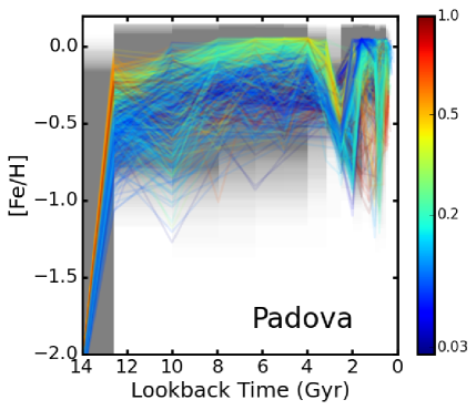
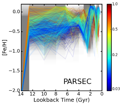
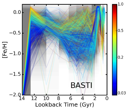
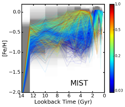
Figure 20.— Metallicity as a function of age for our fits of all regions. Panels are labeled with the models used to obtain the fits. Lines are color-coded by their values in Figure 1.

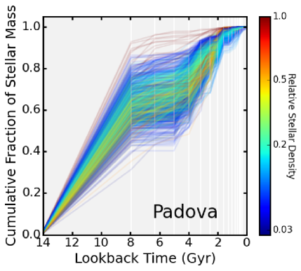
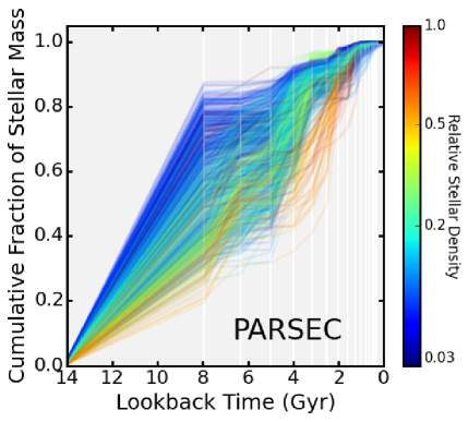
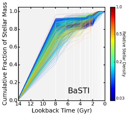
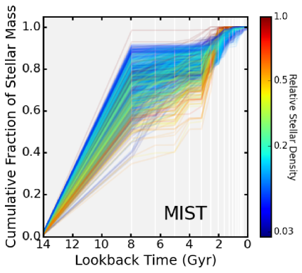
Figure 21.— Cumulative SFH vs. age for different stellar evolution model options. Each panel shows the best-fit cumulative age distribution for all 826 of our sub-regions, color-coded by the stellar density shown in Figure 1. Panels are labeled by with the names of the models used.

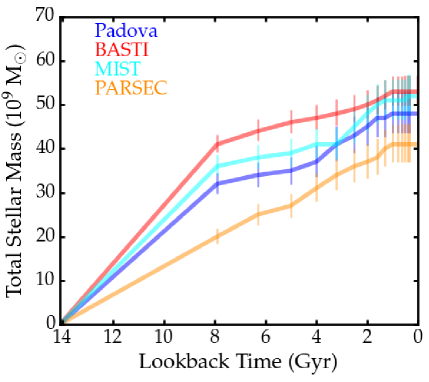
Figure 22.— Total star formation rate vs. age for the entire PHAT footprint, as measured using 3 different model sets imposing a common simple enrichment scenario throughout the survey. The colors show the results for each of the three models sets fitted. Right: Total accumulated mass as a function of lookback time, directly calculated from our fits.

Figure 23.— Total relative star formation rate vs. age for 4 radial bins, color-coded by radius, normalized to have the same mean rate of 1 $M_{\odot}$ yr^-1. These are the results from the Padova model fits.

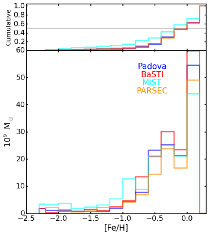
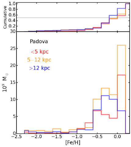
Figure 24.— Metallicity histograms from our free metallicity fits for the entire M31 disk, extrapolated from the entire area measured. The top panel shows the cumulative fraction of the distribution as a function of metallicity. Left: The resulting distribution for all 4 model sets is shown. Right: Metallicity histograms for 3 radial bins from the Padova fits, correcting for area coverage.

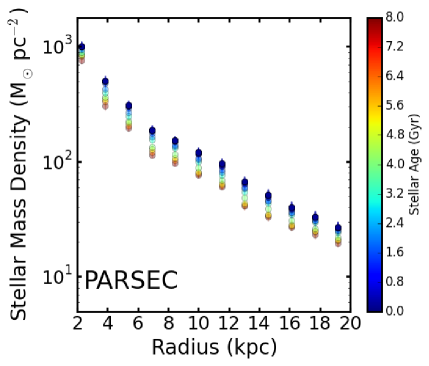
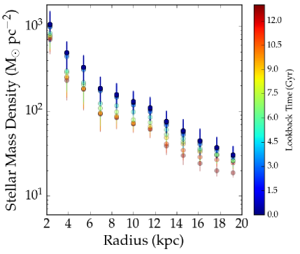
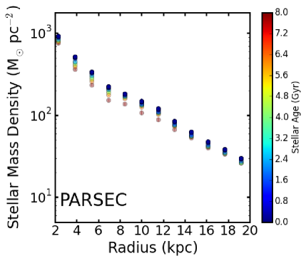
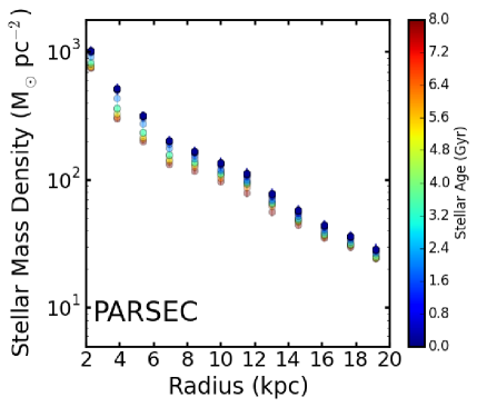
Figure 25.— Cumulative stellar mass surface density formed as a function of radius at several ages (lookback times) for the Padova SFHs shown in Figure 21. Ratios of the results from the Padova SFHs to those from other model sets are provided for comparison. Panels are labeled with the appropriate model set names.

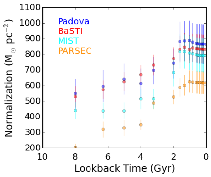
Figure 26.— Exponential fits to the disk profile of M31 as a function of time using the free metallicity fits from the scipy function curve_fit. Left: Disk scale length as a function of lookback time. Right: Normalization of the exponential disk as a function of lookback time.

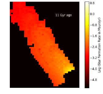
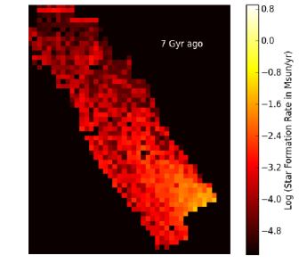
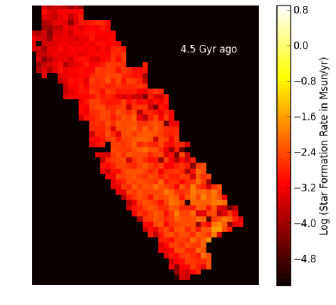
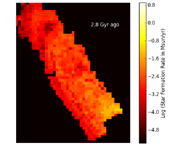
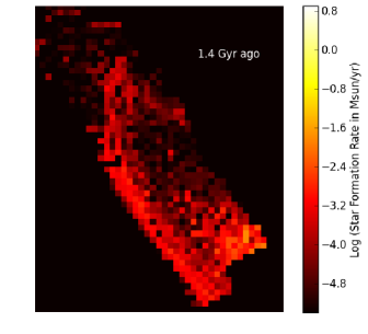
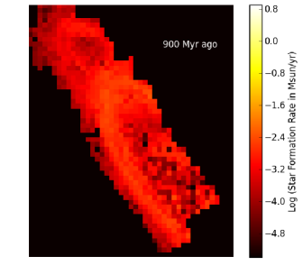
Figure 27.— Subsample of SFH maps from the star formation movie of the PHAT survey.

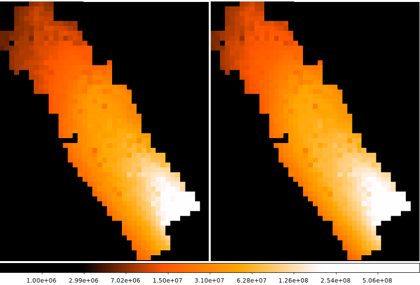
Figure 28.— Total stellar mass as a function of position in the PHAT survey when simple enrichment is assumed. Left: Total stellar mass in each 83${}^{\prime\prime}{\times}83^{\prime\prime}$ region as measured using the Padova models. Right: Same as Left, but as measured using the BaSTI models.

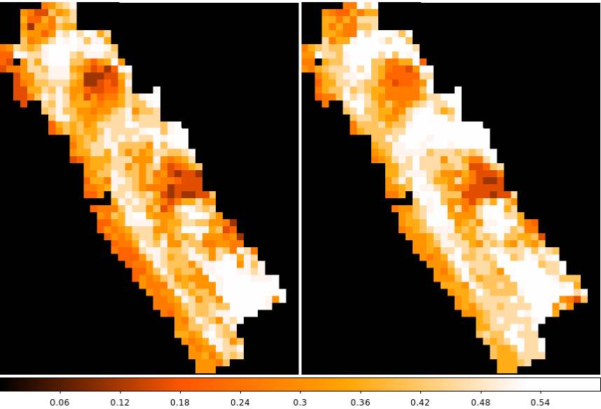
Figure 29.— Maps of the best-fitting foreground $A_{\rm VFG}$ values for the PHAT survey with free metallicity. Left: Foreground $A_{\rm VFG}$ from the Padova fits. Right: Foreground $A_{\rm VFG}$ from the BaSTI fits.

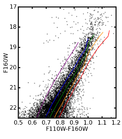
Figure 30.— NIR CMDs of the RGB taken from low (left), medium (middle), and high (right) stellar density regions with very low dust content according to the Dalcanton et al. (2015) maps. Overplotted are Padova 12 Gyr isochrones at a range of metallicities moved to the distance and foreground extinction toward M31. From purple to red the [Fe/H] values are -1.2, -0.8, -0.5, -0.3, and 0.0. There are very few stars with metallicities below -1.0.

References

- Bell et al. (2005) Bell, E. F., et al. 2005, ApJ, 625, 23
- Bellazzini et al. (2003) Bellazzini, M., Cacciari, C., Federici, L., Fusi Pecci, F., & Rich, M. 2003, A&A, 405, 867
- Bernard et al. (2012) Bernard, E. J., et al. 2012, MNRAS, 420, 2625
- Bernard et al. (2015a) Bernard, E. J., Ferguson, A. M. N., Chapman, S. C., Ibata, R. A., Irwin, M. J., Lewis, G. F., & McConnachie, A. W. 2015a, MNRAS, 453, L113
- Bernard et al. (2015b) Bernard, E. J., et al. 2015b, MNRAS, 446, 2789
- Bland-Hawthorn & Gerhard (2016) Bland-Hawthorn, J., & Gerhard, O. 2016, ARA&A, 54, 529
- Blanton & Moustakas (2009) Blanton, M. R., & Moustakas, J. 2009, ARA&A, 47, 159
- Bressan et al. (2012) Bressan, A., Marigo, P., Girardi, L., Salasnich, B., Dal Cero, C., Rubele, S., & Nanni, A. 2012, MNRAS, 427, 127
- Brown et al. (2003) Brown, T. M., Ferguson, H. C., Smith, E., Kimble, R. A., Sweigart, A. V., Renzini, A., Rich, R. M., & VandenBerg, D. A. 2003, ApJ, 592, L17
- Brown et al. (2009) Brown, T. M., et al. 2009, ApJS, 184, 152
- Cassisi et al. (2006) Cassisi, S., Pietrinferni, A., Salaris, M., Castelli, F., Cordier, D., & Castellani, M. 2006, Mem. Soc. Astron. Italiana, 77, 71
- Chemin et al. (2009) Chemin, L., Carignan, C., & Foster, T. 2009, ApJ, 705, 1395
- Chiappini et al. (2001) Chiappini, C., Matteucci, F., & Romano, D. 2001, ApJ, 554, 1044
- Choi et al. (2016) Choi, J., Dotter, A., Conroy, C., Cantiello, M., Paxton, B., & Johnson, B. D. 2016, ApJ, 823, 102
- Cole et al. (2007) Cole, A. A., et al. 2007, ApJ, 659, L17
- Cole et al. (2014) Cole, A. A., Weisz, D. R., Dolphin, A. E., Skillman, E. D., McConnachie, A. W., Brooks, A. M., & Leaman, R. 2014, ApJ, 795, 54
- Courteau et al. (2011) Courteau, S., Widrow, L. M., McDonald, M., Guhathakurta, P., Gilbert, K. M., Zhu, Y., Beaton, R. L., & Majewski, S. R. 2011, ApJ, 739, 20
- Dalcanton et al. (2015) Dalcanton, J. J., et al. 2015, ApJ, 814, 3
- Dalcanton et al. (2012) Dalcanton, J. J., et al. 2012, ApJS, 200, 18
- Dohm-Palmer et al. (2002) Dohm-Palmer, R. C., Skillman, E. D., Mateo, M., Saha, A., Dolphin, A., Tolstoy, E., Gallagher, J. S., & Cole, A. A. 2002, AJ, 123, 813
- Dolphin (2002) Dolphin, A. E. 2002, MNRAS, 332, 91
- Dolphin (2012) Dolphin, A. E. 2012, ApJ, 751, 60
- Dolphin (2013) Dolphin, A. E. 2013, ApJ, 775, 76
- Dolphin et al. (2005) Dolphin, A. E., Weisz, D. R., Skillman, E. D., & Holtzman, J. A. 2005, ArXiv Astrophysics e-prints, astro-ph/0506430
- Dong et al. (2015) Dong, H., Li, Z., Wang, Q. D., Lauer, T. R., Olsen, K. A. G., Saha, A., Dalcanton, J. J., & Williams, B. F. 2015, MNRAS, 451, 4126
- Duane et al. (1987) Duane, S., Kennedy, A. D., Pendleton, B. J., & Roweth, D. 1987, Phys. Lett., B195, 216
- Freeman & Bland-Hawthorn (2002) Freeman, K., & Bland-Hawthorn, J. 2002, ARA&A, 40, 487
- Gallart et al. (2005) Gallart, C., Zoccali, M., & Aparicio, A. 2005, ARA&A, 43, 387
- Girardi et al. (2010) Girardi, L., et al. 2010, ApJ, 724, 1030
- Gregersen et al. (2015) Gregersen, D., et al. 2015, AJ, 150, 189
- Lewis et al. (2015) Lewis, A. R., et al. 2015, ApJ, 805, 183
- MacArthur et al. (2004) MacArthur, L. A., Courteau, S., Bell, E., & Holtzman, J. A. 2004, ApJS, 152, 175
- Marigo et al. (2008) Marigo, P., Girardi, L., Bressan, A., Groenewegen, M. A. T., Silva, L., & Granato, G. L. 2008, A&A, 482, 883
- Mateo (1998) Mateo, M. L. 1998, ARA&A, 36, 435
- McConnachie et al. (2005) McConnachie, A. W., Irwin, M. J., Ferguson, A. M. N., Ibata, R. A., Lewis, G. F., & Tanvir, N. 2005, MNRAS, 356, 979
- McQuinn et al. (2010) McQuinn, K. B. W., et al. 2010, ApJ, 721, 297
- Minchev et al. (2014) Minchev, I., Chiappini, C., & Martig, M. 2014, A&A, 572, A92
- Mollá et al. (1997) Mollá, M., Ferrini, F., & Díaz, A. I. 1997, ApJ, 475, 519
- Naab & Ostriker (2006) Naab, T., & Ostriker, J. P. 2006, MNRAS, 366, 899
- Pietrinferni et al. (2004) Pietrinferni, A., Cassisi, S., Salaris, M., & Castelli, F. 2004, ApJ, 612, 168
- Pietrinferni et al. (2013) Pietrinferni, A., Cassisi, S., Salaris, M., & Hidalgo, S. 2013, A&A, 558, A46
- Rejkuba et al. (2005) Rejkuba, M., Greggio, L., Harris, W. E., Harris, G. L. H., & Peng, E. W. 2005, ApJ, 631, 262
- Rosenfield et al. (2012) Rosenfield, P., et al. 2012, ApJ, 755, 131
- Roškar et al. (2008) Roškar, R., Debattista, V. P., Stinson, G. S., Quinn, T. R., Kaufmann, T., & Wadsley, J. 2008, ApJ, 675, L65
- Saglia et al. (2010) Saglia, R. P., et al. 2010, A&A, 509, A61
- Schlafly & Finkbeiner (2011) Schlafly, E. F., & Finkbeiner, D. P. 2011, ApJ, 737, 103
- Sick et al. (2015) Sick, J., Courteau, S., Cuillandre, J.-C., Dalcanton, J., de Jong, R., McDonald, M., Simard, D., & Tully, R. B. 2015, in IAU Symposium, Vol. 311, Galaxy Masses as Constraints of Formation Models, ed. M. Cappellari & S. Courteau, 82
- Skillman et al. (2014) Skillman, E. D., et al. 2014, ApJ, 786, 44
- Skillman et al. (2017) Skillman, E. D., et al. 2017, ApJ, 837, 102
- Tremonti et al. (2004) Tremonti, C. A., et al. 2004, ApJ, 613, 898
- Weisz et al. (2011) Weisz, D. R., et al. 2011, ApJ, 739, 5
- Williams (2002) Williams, B. F. 2002, MNRAS, 331, 293
- Williams (2003) Williams, B. F. 2003, AJ, 126, 1312
- Williams et al. (2012) Williams, B. F., et al. 2012, ApJ, 759, 46
- Williams et al. (2015) Williams, B. F., et al. 2015, ApJ, 806, 48
- Williams et al. (2011) Williams, B. F., et al. 2011, ApJ, 734, L22
- Williams et al. (2009) Williams, B. F., et al. 2009, AJ, 137, 419
- Williams et al. (2014) Williams, B. F., et al. 2014, ApJS, 215, 9
- Young et al. (2007) Young, L. M., Skillman, E. D., Weisz, D. R., & Dolphin, A. E. 2007, ApJ, 659, 331