Exact probability distribution function for the volatility of cumulative production

Abstract

In this paper we study the volatility and its probability distribution function for the cumulative production based on the experience curve hypothesis. This work presents a generalization of the study of volatility in Lafond , which addressed the effects of normally distributed noise in the production process. Due to its wide applicability in industrial and technological activities we present here the mathematical foundation for an arbitrary distribution function of the process, which we expect will pave the future research on production and market strategy.

Introduction

Understanding the volatile behaviour of industrial activities and the complexity related to them, intrigues many researchers. One of the stylized facts for describing this phenomenon is a well known experience curve. The concept of experience curves and empirical evidence for them were presented in Wright’s Wright seminal paper, in which he first discovered the relationship of cost and quantity. Wright’s curve is known in the literature as “learning curve”, as it is based on “the more learning by more producing hypothesis”, for describing the price-experience relationship. Wright realized that empirically the reduction of cost followed a constant proportion rate, as the production duplicated. In other words, the higher the experience in producing a specific product is, the lower its costs are, when the inflation is factored out.

The inspiration of this paper comes from the fact that the experience curves hypothesis can provide a significant understanding of the market strategy, for instance export potentials due to the knowledge of experience levels, the prediction of future prices, given some information about the market costs decrease by some consistent rate of decline, the applicability in risks management, etc. (Note that the notion is suitable for cost control or forecasting over long range strategic development).

The phenomenon depends on some crucial factors, i.e. competent management, technological improvement, etc. Furthermore there must be a characteristic pattern that causes this phenomenon, for instance a better development of better tools, automatization, training programs Terwiesch ; Vits ; Serel ; Azizi , prior experience and the work complexity task Nembhard ; Pananiswami .

The notion of experience curve could also describe the effect between business competitors, for example, who is faster by reducing the costs, which is an example of complex systems interactions and network.

There is a vast literature on empirical information about the experience curves, including a wide range of industrial activities, see e.g. Arrow . The aforementioned work had a major impact on the development of this concept, by arguing that technical learning was a result of experience gained, based on the idea learning by doing. Some researchers question its usefulness for forecasting and planning the deployment of industrial and technological activities Lafond ; Ayres ; Anzanello ; Sahal ; Martino . In the aforementioned literature it has been found that experience curves can be used to estimate future technology costs, considering the shape of the forecast error distribution. (Note the finding depends on some parameters, for instance the length and the period of observed time series).

Despite the wide variety of empirical evidence of the experience curves, there is a lack of theoretical and mathematical framework of the concept. Motivated by this fact and by the fact that there exists a large number of cases where the distribution describing a complex phenomenon is not Gaussian, e.g. the price fluctuations of most financial assets Bouchaud , in this paper we present a theoretical, mathematical framework for describing a probability distribution function of the volatility of the cumulative production for an arbitrary probability distribution of noise. In analogy to the concept of learning curves, which is a relation between the input and the output of a learning process, one of our main findings shows the relation between previous and next probability distribution functions which characterizes their volatility.

Knowing distribution functions of the cumulative production and its volatility allows us to understand the complex behaviour of the system and to calculate the various quantities, such as mean, variance and also higher order moments, price volatility correlation, etc.

Volatility for narrow distributions

It was first discovered by Sahal Sahal that the exponentially increasing cumulative production and exponentially decreasing costs gives an experience curve law, which indicates a linear relationship between cost and increment of cumulative production.

Similar to Lafond , let us consider that empirically cumulative production growth follows a smooth exponential behaviour in the presence of noise, by assuming that production is a geometric random walk with drift $g$ and variance $\sigma_{a}^{2}$. Within this model, cumulative production is given by:

$$Z{{}_{t}}=\sum_{j=0}^{t}{{\rm e}^{gj}{{\rm e}^{a_{1}}...{\rm e}^{a_{j}}}},$$ (1)

where $a_{1},a_{2}$, … are stochastic i.i.d. variables, which describe the presence of noise in the production process.

Let us first consider the special case, where $a_{1},a_{2}$, … are normally distributed i.i.d. variables, with mean zero and variance $\sigma_{a}^{2}$. For the calculation of cumulative production and its volatility in Lafond the saddle point method was used. The main idea of the saddle point is to approximate an integral by taking into account only the range of the integration where the integrand takes its maximum. A priory, this can only be correct for small variance $\sigma_{a}^{2}$.

In Lafond first the expectation value of cumulative production and its variance were calculated, which lead to the multiple integral over $a_{i}$

$$E(\log Z) =\int_{-\infty}^{\infty}\log Z\prod_{i=1}^{t}\frac{da_{i}}{\sqrt{2\pi\sigma_{a}^{2}}}\exp\Big{[}-\frac{a_{i}^{2}}{2\sigma_{a}^{2}}\Big{]}$$ (2)

$$=\int_{-\infty}^{\infty}\prod_{i=1}^{t}\frac{da_{i}}{\sqrt{2\pi\sigma_{a}^{2}}}{\rm e}^{S(\{a_{i}\})},$$

with $S(\{a_{i}\})=\log(\log Z)-\sum_{i=1}^{t}\frac{a_{i}^{2}}{2\sigma_{a}^{2}}$.

For $\sigma_{a}^{2}\ll 1$ the saddle point method yields explicit results, for instance the variance of $\log Z(t)$

$$\mbox{Var}(\log Z(t)) =E(\log^{2}Z)-E(\log Z)^{2}$$ (3)

$$=\sigma_{a}^{2}\left(\frac{2{\rm e}^{g}+1}{1-{\rm e}^{2g}}+t\right)+O(\sigma_{a}^{4}).$$

Finally, the main result of this method is volatility, i.e. the variance of volatility variable $\Delta\log Z:=\log Z_{t}-\log Z_{t-1}$ for large time $t\rightarrow\infty$ and is given by the following expression (valid for $g>0$ and small $\sigma_{a}^{2}$):

$$\mbox{Var}(\Delta\log Z) =\sigma_{a}^{2}\tanh\left(\frac{g}{2}\right)+O(\sigma_{a}^{4}).$$ (4)

For details of the derivation we refer to Lafond . Since $\tanh\left(\frac{g}{2}\right)<1$ we have always $\mbox{Var}(\Delta\log Z)<\sigma_{a}^{2}$ an inequality, which means the volatility of cumulative production is lower than the volatility of production. We have tested this remarkably simple, but potentially powerful relationship using empirically available data and we found that it works reasonably well.

Volatility for the general case

The core result of this paper is the investigation of the volatility of cumulative production for more general distribution functions of $a_{i}$ than considered in Lafond . Let us assume that in Eq. ($1$), $a_{1}$, $a_{2}$, … are stochastic i.i.d. variables which are distributed according to some distribution function $\rho_{a}$ of any shape and width.

We are interested in the distribution function of the cumulative production $z_{t}:=\log Z_{t}$ which we call $\rho_{z_{t}}$. From this distribution function we can calculate all important characteristic quantities of the system. Surprisingly, the distribution function can be shown to satisfy a useful recursion relation for successive times:

$$\rho_{z_{t+1}}(x)=\frac{1}{1-\exp(-x)}.\\ \rho_{a}*\rho_{z_{t}}(\log(\exp(x)-1)-g).$$ (5)

The detailed derivation can be found in Appendix A.

Generally Eq. (5) has to be solved numerically by recursions. Numerical analyses can be done to high accuracy and completely replace simulations, which are time consuming and sometimes inaccurate.

It is possible to obtain analytic results at least for two cases. In the case of a distribution of $\rho_{a}$ with main weight around some $x_{0}$ and a value of $g$ such that $g+x_{0}>0$ we find for large $t$ an asymptotic solution. In this case only large values of $x$ matter and (5) linearizes to $\rho_{z_{t+1}}(x)=\rho_{a}*\rho_{z_{t}}(x-g)$. The second case is a narrow distribution of $\rho_{a}$, which we comment later.

Eq. (5) is highly useful in numerical calculations, especially because the convolution integral can be carried out efficiently and the convergence for increasing time is fast. Of course it would be desirable to treat the time evolution of the probability distribution function for arbitrary $t$ fully analyticaly such as in Zadourian . The analytical solution is the subject of current investigation.

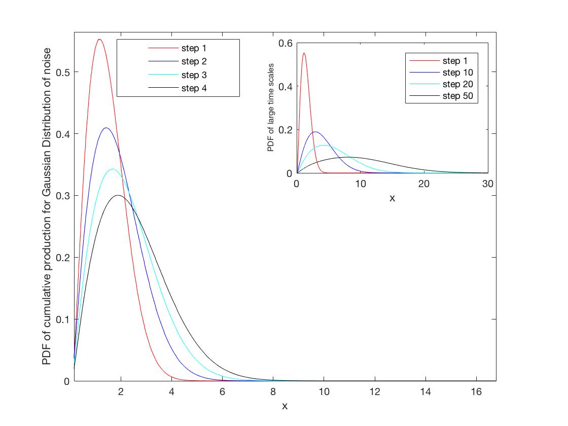
Figure 1: Plot of probability distribution functions of $\log Z_{t}$ of the Gaussian distributed $\rho_{a}$ for different time steps, where $g=0.2$ and $\sigma_{a}=1$ are chosen. The inset shows curves on a large time scale.

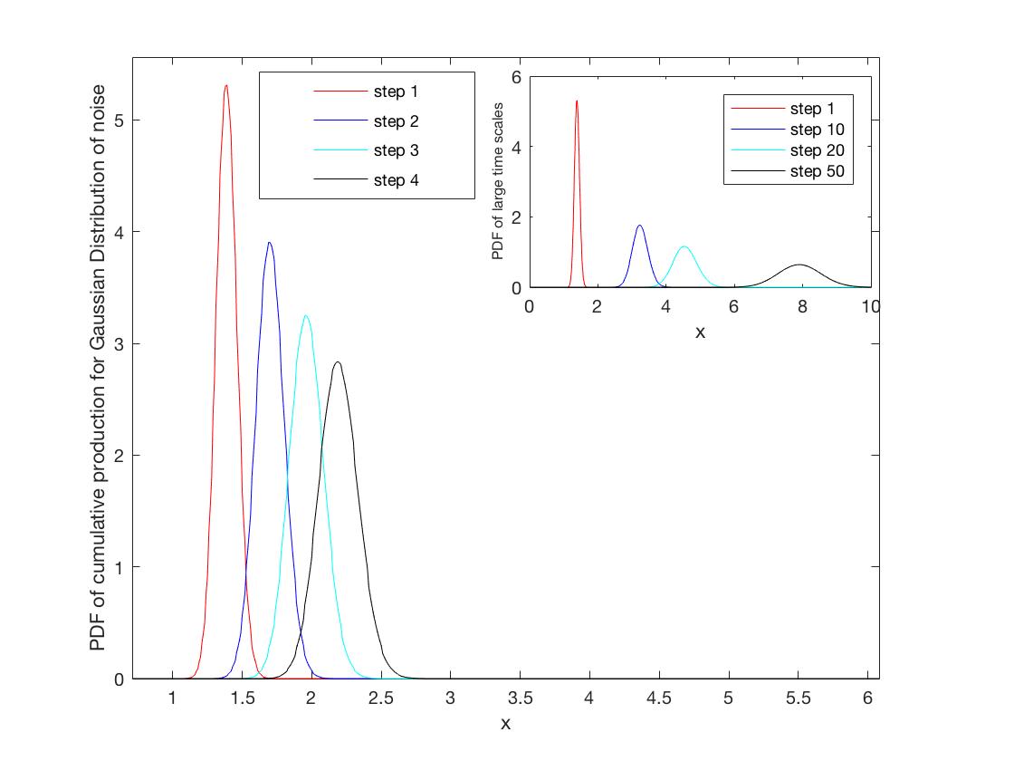
Figure 2: Plot of probability distribution functions of $\log Z_{t}$ of Gaussian distributed noise for different time steps, where $g=0.2$ and $\sigma_{a}=0.1$ are chosen. The inset shows curves on a large time scale.

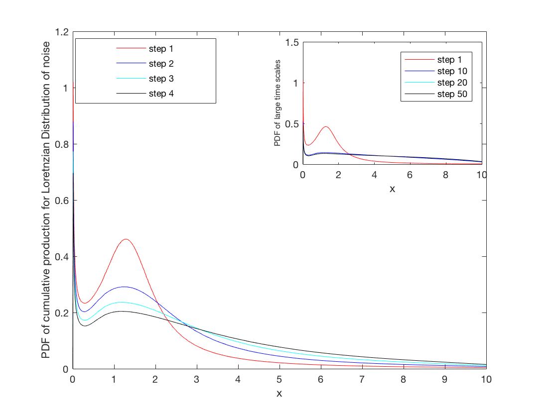
Figure 3: Plot of probability distribution functions of $\log Z_{t}$ of Lorentzian distributed noise for different time steps, where $g=0.2$ and width equal to 1 are chosen. The inset shows curves on a large time scale.

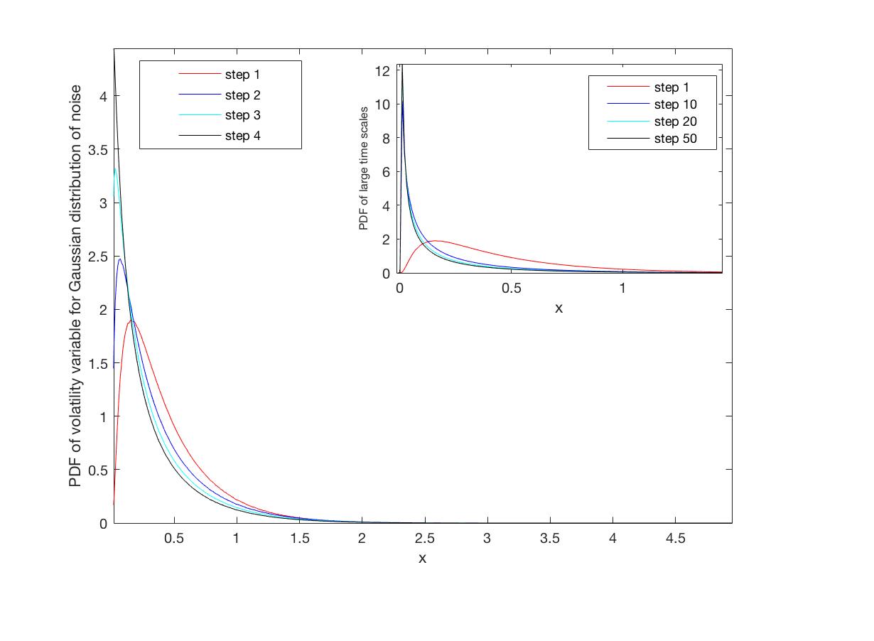
Figure 4: Plot of probability distribution functions of the volatility variable for the Gaussian case for $\rho_{a}$ and different time steps, where $g=0.2$ and $\sigma_{a}=1$. The Inset is considered for a large time scale.

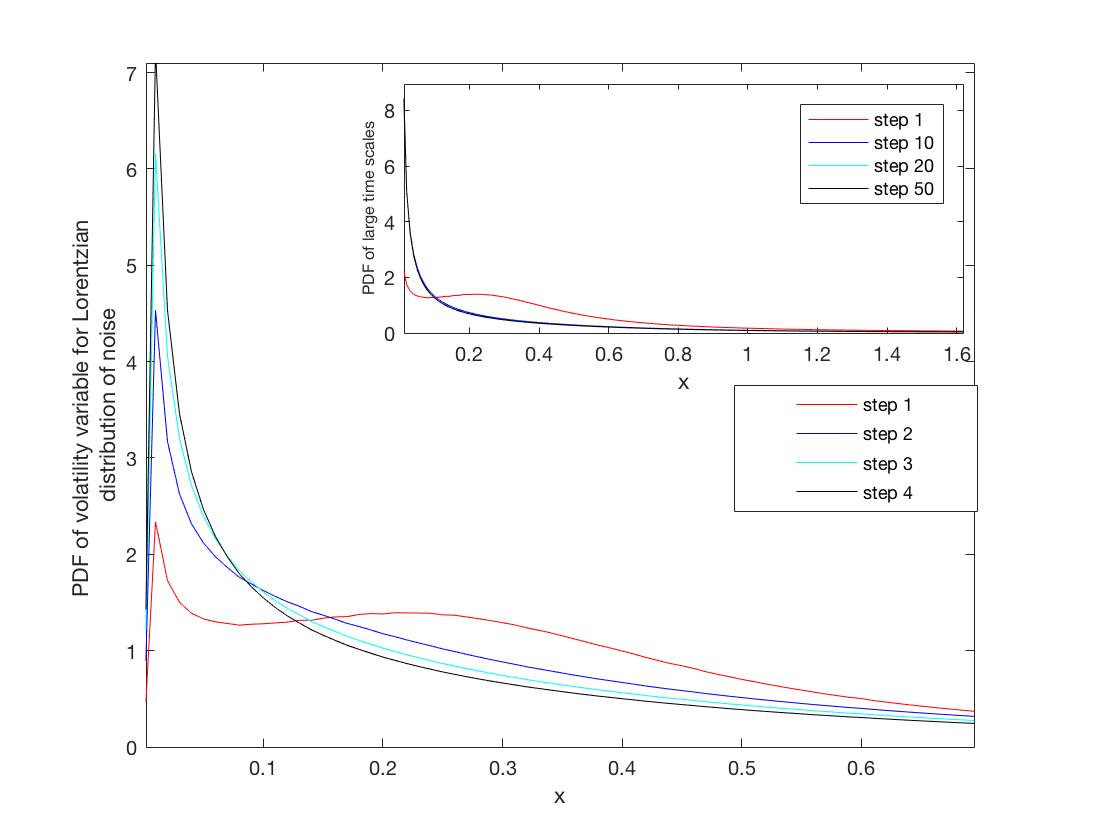
Figure 5: Plot of probability distribution functions of the volatility variable for the Lorentzian case for $\rho_{a}$ and different time steps, where $g=0.2$ and width is equal to 1. The inset shows curves on a large time scale.

Fig. $1$, $2$ and $3$ show the distributions of cumulative production for different types of noise and several time steps.

The distribution of volatility

The quantity of our interest is the volatility, which is by definition the variance of the distribution function $z_{t}-z_{t-1}$. We observe

$$\Delta{z_{t}} := z_{t}-z_{t-1}=\log Z_{t}-\log Z_{t-1}$$ (6)

$$= -\log\left(1-\frac{Z_{t}-Z_{t-1}}{Z_{t}}\right).$$

We define:

$$Y_{t}:=\frac{Z_{t}}{Z_{t}-Z_{t-1}}.$$ (7)

In Appendix B we show $Y_{t}$ is distributed as $Z_{t}$ in Eq. ($1$) with $g\to-g$ and $a_{i}\to-a_{i}$, see Eq. (22).

From the above expression we get the following result for the distribution function of the variable $y_{t}=\log{Y_{t}}$:

$$\rho_{\Delta{z_{t}}}(x)=\frac{1}{\exp(x)-1}\rho_{y_{t}}(-\log(1-\exp(-x))),$$ (8)

where $\rho_{y_{t}}$ satisfies the same recursion as $\rho_{z_{t}}$, after changing the signs of $g$ and $a_{i}$, as mentioned above.

The detailed explanation of Eq. $(\ref{eqnine})$ can be found in Appendix B.

Figs. $4$ and $5$ illustrate volatility distributions $\rho_{\Delta{z_{t}}}$, considering for $\rho_{a}$ normal and lorentzian distributions. The Figures show the different behaviours of $\rho_{z_{t}}(x)$, with singular (but integrable) characteristics at $x=0$ for i.e. $g\geq 0$. The first few time steps show sizable changes whereas only small changes happen at larger times.

In order to demonstrate the usefulness of Eq. (5) and (8), let us derive from it Eq. (4), which is the result of the saddle point approximation: we take for $\rho_{a}$ a narrow distribution with $0$ mean and (small) variance ${\sigma_{a}^{2}}$ and accordingly ${\bar{y}_{t}}=\log(\sum_{j=0}^{t}{\rm e}^{-jg})$ and ${\sigma_{t}^{2}}$ are the mean and the (to be calculated) variance of the narrow $\rho_{y_{t}}$ distribution. Using variable transformation and the nice property of additivity of the variance under convolution we obtain the derivation of the volatility for the special case in Eq. (4). We defer the detailed derivation of the above statement to Appendix C.

We also compared our numerical results for general values of $\sigma_{a}^{2}$ with the saddle point result obtained in Eq. $(4)$. These analyses show that the general treatment of the probability distributions and the saddle point approximation coincide for small variance $\sigma_{a}^{2}$.

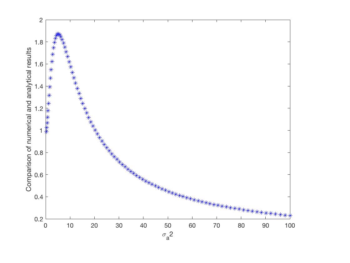
Figure 6: Plot of the ratio of the numerically exact value of volatility and the saddle point approximation versus various values of the variance ${\sigma_{a}}^{2}$ of noise, by fixed drift, $g=0.1$.

Fig.6 shows that for small values of $\sigma_{a}$ the analytical approximation and the numerical results coincide whereas for larger $\sigma_{a}$ we see sizable deviations. The volatility for intermediate (large) values of $\sigma_{a}$ takes larger (smaller) values than the result of the saddle point approximation.

summary

The concept of experience curves has been widely used in different domains, such as industrial engineering and operations management services, aimed to estimate the future costs, to reduce the production costs, to evaluate workers’ learning profile, etc. It plays also a major role in some strategic tasks, related to capacity, pricing and employment.

Furthermore there exists a large number of cases where the distribution describing a complex phenomenon is not Gaussian. For this variety of applications we found a comprehensive analytical approach, which is based on the probability distribution function of the model. We derived a recursion relation of integral type that replaces simulations by highly accurate numerical integration. The results show how different types of noise affect the cumulative production within the model, based on the learning by doing hypothesis. The distribution functions of the volatility are hardly characterized by the mean and variance and show rather interesting, sometimes singular behaviour.

Knowing such an important quantity fosters a deeper understanding of the industrial activities. It also allows us to understand the volatile and complex feature of the system and accordingly to calculate the significant quantities, by envisioning the opportunities of the model for future investigations in risk management.

* * *

RZ thanks J. Doyne Farmer and Francois Lafond for support and discussions.

Appendix A: Derivation of the distribution function $\Delta{\rho_{z_{t}}}$

Here we will derive the recursion expression (5). Note that the modified object

$$\tilde{Z}_{t}:=\sum_{j=0}^{t}{\rm e}^{gj}{\rm e}^{a_{2}}...{\rm e}^{a_{j+1}}$$ (9)

has the same distribution function as $Z_{t}$, because we have used different, but independent and identically distributed $a_{i}$’s. So $\tilde{z}_{t}:=\log\tilde{Z}_{t}$ is distributed according to $\rho_{\tilde{z}_{t}}=\rho_{z_{t}}$. Note that

$$1+{\rm e}^{g+a_{1}}\tilde{Z}_{t}=1+\sum_{j=0}^{t}{\rm e}^{g(j+1)}{\rm e}^{a_{1}}{\rm e}^{a_{2}}...{\rm e}^{a_{j+1}}\\ =1+\sum_{i=1}^{t+1}{\rm e}^{gi}{\rm e}^{a_{1}}{\rm e}^{a_{2}}...{\rm e}^{a_{i}}=Z_{t+1}.$$ (10)

Therefore we have

$$z_{t+1}=\log(1+\exp(g+a_{1}+\tilde{z}_{t})=f(g+a_{1}+\tilde{z}_{t})$$ (11)

where we have used the definition of the function $f$:

$$f(x):=\log(1+\exp(x)).$$ (12)

The stochastic variable $a_{1}+\tilde{z}_{t}$ is distributed according to the convolution of $\rho_{a}$ with $\rho_{z_{t}}$. The distribution of $g+a_{1}+\tilde{z}_{t}$ is the convolution with a subsequent shift of the argument:

$$\rho_{a_{1}+\tilde{z}_{t}}=\rho_{a_{1}}*\rho_{\tilde{z}_{t}}=\rho_{a}*\rho_{z_{t}},$$

$$\rho_{g+a_{1}+\tilde{z}_{t}}(x)=\rho_{a}*\rho_{z_{t}}(x-g).$$ (13)

With (11) and (13) we can calculate the distribution function $\rho_{z_{t+1}}$ of $z_{t+1}$. If we use the arguments $x$ for $\rho_{g+a_{1}+\tilde{z}_{t}}$ and $y=f(x)$ for $\rho_{z_{t+1}}$ we find

$$\rho_{z_{t+1}}(y)dy=\rho_{g+a_{1}+\tilde{z}_{t}}(x)dx,$$ (14)

and from this

$$\rho_{z_{t+1}}(y)=[f^{\prime}(x)]^{-1}\rho_{g+a_{1}+\tilde{z}_{t}}(x)\\ =[f^{\prime}(x)]^{-1}\rho_{a}*\rho_{z_{t}}(x-g).$$ (15)

Now we use $f^{\prime}(x)=\exp(x)/(1+\exp(x))$ and $x=f^{-1}(y)=\log(\exp(y)-1)$ and reach one of our main findings:

$$\rho_{z_{t+1}}(x)=\frac{1}{1-\exp(-x)}.\\ \rho_{a}*\rho_{z_{t}}(\log(\exp(x)-1)-g).$$ (16)

Appendix B: Derivation of the distribution function of the volatility variable $\Delta z_{t}$

According to the definition of $Y_{t}$ we have $Y_{t}=\frac{Z_{t}}{Q_{t}}$, with

$$Z_{t}:=\sum_{j=0}^{t}Q_{j},\qquad Q_{j}:={\rm e}^{gj}{\rm e}^{a_{1}}...{\rm e}^{a_{j}}$$ (17)

where $g$ is a constant, and $a_{1}$, $a_{2}$, … are stochastic i.i.d. variables which are distributed according to some distribution function $\rho_{a}$. Now – luckily – $Y_{t}$ has the same structure as $Z_{t}$ if we replace the constant $g$ and the stochastic variables $a_{i}$ by $g$ and $-a_{i}$:

$$Y_{t}:=\frac{Z_{t}}{Q_{t}}=\sum_{j=0}^{t}\frac{Q_{j}}{Q_{t}},\qquad\frac{Q_{j}}{Q_{t}}={\rm e}^{g(j-t)}{\rm e}^{-a_{j+1}}...{\rm e}^{-a_{t}}$$ (18)

Next we define

$$\tilde{g}:=-g,\qquad\tilde{a}_{1}:=-a_{t},\quad\tilde{a}_{2}:=-a_{t-1},\quad...,\\ \tilde{a}_{t}:=-a_{1}$$ (19)

And indeed

$$\frac{Q_{j}}{Q_{t}}={\rm e}^{g(j-t)}{\rm e}^{-a_{j+1}}...{\rm e}^{-a_{t}}={\rm e}^{\tilde{g}(t-j)}{\rm e}^{\tilde{a}_{1}}...{\rm e}^{\tilde{a}_{t-j}}$$ (20)

Hence

$$Y_{t}=\sum_{j=0}^{t}{\rm e}^{\tilde{g}(t-j)}{\rm e}^{\tilde{a}_{1}}...{\rm e}^{\tilde{a}_{t-j}}=\sum_{j=0}^{t}{\rm e}^{\tilde{g}j}{\rm e}^{\tilde{a}_{1}}...{\rm e}^{\tilde{a}_{j}}$$ (21)

As mentioned above we find that the distribution function of $y_{t}:=\log{Y_{t}}$ corresponds to that of $z_{t}:=\log{Z_{t}}$, by taking into account sign changes of $g$ and $a_{i}$. Hence it satisfies the recursion relation derived in App. A:

$$\rho_{y_{t+1}}(x)=\frac{1}{1-\exp(-x)}.\\ \rho_{-a}*\rho_{y_{t}}(\log(\exp(x)-1)+g).$$ (22)

Appendix C: Analytic treatment of narrow distributions

For obtaining the saddle point formula Eq. (4) from the general recursion relation we need to recall Eqs. (5) and (22). $\rho_{a}$ is given by a narrow distribution around $0$ and variance ${\sigma_{a}}^{2}$ and correspondigly $\rho_{y_{t}}$ is defined by the mean ${\bar{y}_{t}}=\log(\sum_{j=0}^{t}{\rm e}^{-jg})$ and ${\sigma_{t}}^{2}$.

Due to the additivity feature of the variance under convolution, the narrow $\rho_{a}*\rho_{y_{t}}$ has the variance equal to ${\sigma_{t}}^{2}+{\sigma_{a}}^{2}$.

Let us use the variable transformation in Eq. (22). Then we get ($\sigma_{t}:=\sigma_{y_{t}}$)

$$\frac{d(\log({\rm e}^{x}-1)+g)}{dx}{\sigma_{t+1}}=\sqrt{{\sigma_{t}}^{2}+{\sigma_{a}}^{2}},$$ (23)

where $x=\bar{y}_{t}$. For large times $t\to\infty$ we get

$${\sigma_{\infty}}^{2}=\frac{1}{{\rm e}^{2g}-1}{\sigma_{a}}^{2}.$$ (24)

Let us now calculate the main result, namely $\sigma_{\Delta{z_{t}}}$, the volatility for narrow distributions. To this end we need to transform variables in Eq. (5)

$$\sigma_{\Delta{z_{t}}}=({\rm e}^{x}-1){\sigma_{t}}$$ (25)

For $x$ equal to its maximum we have:

$$-\log(1-{\rm e}^{-x})=\bar{y}_{t}$$ (26)

and for $t\to\infty$ this amounts to $x=g$.

Finally, we obtain the result for the special, narrow distributed function, which in the previous work Lafond was obtained by the saddle point approximation.

$$\sigma_{\Delta{z_{t}}}=\sqrt{\tanh{(\frac{g}{2}})}{\sigma_{a}}.$$ (27)

References

- (1) Francois Lafond, Aimee Gotway Bailey, Jan David Bakker, Dylan Rebois, Rubina Zadourian, Patrick McSharry and J. Doyne Farmer, How well do experience curves predict technological progress? A method for making distributional forecasts. arXiv:1703.05979 (2017)
- (2) T.P. Wright, Factors Affecting the Cost of Airplanes, Journal of the Aeronautical Sciences, February, Vol. 3, No. 4 : pp. 122-128
- (3) Terwiesch, C., Bohn, R., 2001. Learning and process improvement during production ramp-up. International Journal of Production Economics 70 (1), 1-19.
- (4) Vits, J., Gelders, L., 2002. Performance improvement theory. International Journal of Production Economics 77 (3), 285-298.
- (5) , Serel D.A., Dada, M., Moskowitz, H., Plante, R.D., 2003. Investing in quality under autonomous and induced learning. IIE Transactions 35 (6), 545-555.
- (6) Azizi, N., Zolfaghari, S., Liang, M., 2010. Modeling job rotation in manufacturing systems: the study of employee’s boredom and skill variations. International Journal of Production Economics 123 (1), 69-85.
- (7) Nembhard, D.A., Osothsilp, N., 2002. Task complexity effects on between-individual learning/forgetting variability. International Journal of Industrial Ergonomics 29 (5), 297-306.
- (8) Pananiswami, S., Bishop, R.C., 1991. Behavioral implications of the learning curve for production capacity analysis. International Journal of Production Economics 24 (1e2), 157e163.
- (9) Arrow, K. J. (1962), The economic implications of learning by doing, The Review of Economic Studies pp. 155–173.
- (10) Farmer J. D. and Lafond, F. (2016), How predictable is technological progress?, Research Policy 45(3), 647–665.
- (11) Ayres, R. U. (1969), Technological forecasting and long-range planning, McGraw-Hill Book Company.
- (12) Michel Jose Anzanello, Flavio Sanson Fogliatto , Learning curve models and applications: Literature review and research, International Journal of Industrial Ergonomics, 41 (2011) 573-583 directions
- (13) Sahal, D. (1979), theory of progress functions, AIIE Transactions 11(1), 23–29.
- (14) Martino J. P. (1993), Technological forecasting for decision making, McGraw-Hill, Inc.
- (15) J.-P. Bouchaud and M. Potters, Theory of Financial Risk and Derivative Pricing: From Statistical Physics to Risk Management (Cambridge Univ. Press, Cambridge U.K., 2003).
- (16) Rubina Zadourian, David B. Saakian, and Andreas Klümper, Exact probability distribution functions for Parrondo’s games, Phys. Rev. E94, (2016)