Tracing the evolution of nuclear forces under the similarity renormalization group

Abstract

I examine the evolution of nuclear forces under the similarity renormalization group (SRG) using traces of the many-body configuration-space Hamiltonian. While SRG is often said to “soften” the nuclear interaction, I provide numerical examples which paint a complementary point of view: the primary effect of SRG, using the kinetic energy as the generator of the evolution, is to shift downward the diagonal matrix elements in the model space, while the off-diagonal elements undergo significantly smaller changes. By employing traces, I argue that this is a very natural outcome as one diagonalizes a matrix, and helps one to understand the success of SRG.

Introduction. Nuclear structure theory has undergone a renaissance, driven by advances in high performance computing as well as by rigorous and systematic methodologies for both ab initio nuclear forces, such as chiral effective field theory[1, 2, 3] and for application of those forces to many-body calculations. Included in the latter are the no-core shell model [4, 5] and the similarity renormalization group [6, 7, 8, 9, 10], which together have been very successful in calculating properties of light nuclei starting primarily from two-nucleon data. It is often said that the similarity renormalization group (SRG) “softens” the nuclear interaction, improving convergence with model space size. In this short paper I demonstrate that, at a gross level, the dominant effect of SRG on no-core shell model (NCSM) calculations is to shift low-lying energies down, with much smaller effects on wave functions. Using traces over the many-body model space, I argue that, in retrospect, the weakening of off-diagonal matrix elements and a much larger downward shift in diagonal elements go hand-in-hand.

The no-core shell model is a configuration-interaction method, whereby one solves the nonrelativistic nuclear Schrödinger equation $\hat{H}|\Psi_{i}\rangle=E_{i}|\Psi_{i}\rangle$ as a matrix eigenvalue problem, typically in a basis of Slater determinants, that is, antisymmetrized products of single-particle states in the lab frame. An important goal of modern nuclear structure theory is to carry out many-body calculations, in the NCSM or other methodologies, using nucleon-nucleon forces fitted with high precision to experimental phase shifts [11, 12, 13]. These forces are generated in relative coordinates and then transformed to the lab frame via Talmi-Moshinsky-Brody brackets [14, 15, 16]. Now come two crucial concepts I rely upon. The first is that finding eigenpairs involves a unitary transformation to a diagonal matrix. (Because one only wants low-lying eigenpairs and not all of them, one uses the Lanczos algorithm [17], but the basic idea remains.) To diagonalize the “full” matrix is impractical, hence we must diagonalize in a smaller, truncated model space. Yet ab initio nuclear forces have large matrix elements connecting states of low and high relative momentum, which historically and phenomenologically was interpreted as a hard repulsive core. In the shell model configuration basis this “hard core” becomes a strong coupling between the truncated model space and the excluded space, driving the inclusion of many configurations to converge results as a function of model space size, typically described by $N_{\mathrm{max}}$ (the number of excitations in an noninteracting harmonic oscillator space).

In order to improve solutions in the model space, one turns to effective interaction theories. Most of these are unitary or quasi-unitary transformations, and one of the most widely applied is the similarity renormalization group, where one evolves a Hamiltonian by the differential equation

$$\frac{d}{ds}\hat{H}(s)=\left[\hat{H}(s),\left[\hat{H}(s),\hat{G}\right]\right].$$ (1)

Here $\hat{G}$ is the generator of the evolution and is often picked to be the kinetic energy $\hat{T}$. If fully carried out, (1) is a unitary transformation of the Hamiltonian. (It also induces, however, many-body forces [9, 18], and as one typically carries out (1) in just the two- or three-body systems, higher rank forces are dropped and one has a loss of unitarity. A closely related methodology is the in-medium SRG[19, 20], which by normal ordering approximately accounts for higher rank forces, although I do not consider it further.) In other words, when a matrix is diagonal, each eigenstate is decoupled from all the rest, while SRG and related techniques seek to improve the solution in the model space by approximately decoupling the model space from the excluded space. In what follows I will gives examples of the effect of SRG on solutions in the model space, and then interpret those effects in terms of traces on the many-body Hamiltonian matrix.

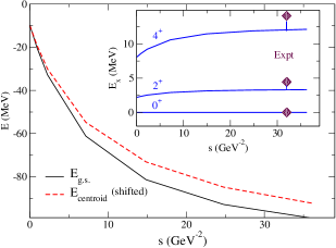
Figure 1: (Color online) Evolution under the similarity renormlization group of ground state energy of ¹²C (black solid line) and excitation energies of the first $2^{+}$, $4^{+}$ states (inset), where the (maroon) diamonds show the experimental values for comparison. The calculations were carried out in an $N_{\mathrm{max}}=8$ many-body space in a harmonic oscillator basis frequency of $\hbar\Omega=20$ MeV, using the Entem-Machleidt chiral effective interaction evaluated to N3LO. Also shown (red dashed line) is the evolution of the energy of the centroid, as defined in Eq. (3); the centroid energy is shifted down by 221.88 MeV to show it tracking the ground state energy.

As an example of the NCSM using SRG-evolved forces, I consider ¹²C in a Slater determinant (lab frame) basis built from single-particle harmonic oscillator states with $\hbar\Omega=20$ MeV, allowing up to $N_{\mathrm{max}}=8$ excitations; such a space allows one to exactly separate out spurious center-of-mass motion using the Palumbo-Glockle-Lawson method [21, 22]. The interaction was derived in chiral effective field theory in next-to-next-to-next-to-leading order [13] or N3LO; it was then evolved in relative momentum space via SRG (with the kinetic energy as the generator $\hat{G}$ in Eq. (1)) to various values of $s$, and then transformed to the lab frame via Talmi-Moshinsky-Brody brackets [14, 15, 16]. (The representation of the interaction in relative coordinates has a finite cut-off; in harmonic oscillator states it is typically truncated at 100-300 $\hbar\Omega$ [5], which corresponds to $N_{\mathrm{max}}\sim 100$-$300$. In the lab frame, the non-spurious many-body states are coupled to the ground state of center-of-mass motion. Thus the non-spurious Hamiltonian in a many-body basis in the lab frame is also finite, though $N_{\mathrm{max}}\sim 100$-$300$ is much larger than any configuration-interaction code can fully handle, and so the Hamiltonian in single-particle coordinates, or the lab frame, is always truncated.) Often one reinterprets the evolution in terms of a wavenumber cutoff, $\lambda=\frac{\sqrt{M_{N}}}{\hbar}s^{-1/4}$, which has units of fm^-1; here $M_{N}$ is the nucleon mass. Although $\lambda$ suggests the “resolution” of the renormalized interaction, I retain $s$ to emphasize the evolutionary nature of SRG, so that $s=0$ is the original or unevolved interaction; this corresponds to $\lambda=\infty$. The shell model calculations are carried out using the BIGSTICK code [23].

Fig. 1 shows how the ground state energy plunges as one goes from the bare force, $s=0$, to one evolved to $s$= 36.3 GeV^-2 which is equivalent to $\lambda=2.0$ fm^-1. While the ground state energy changes by nearly 90 MeV, the inset shows the excitation energies change hardly at all. Table 1 shows $\Delta E_{g.s.}=E_{g.s.}(s=0)-E_{g.s.}(s=36.3\,\mathrm{GeV}^{-2})$, the change in the ground state energy under SRG, for several different $p$-shell nuclides, including different $N_{\mathrm{max}}$ truncations.

Table 1: Changes in ground state energies and centroids for selected $p$-shell nuclides, including for different $N_{\mathrm{max}}$ truncations, under SRG evolution from $s=0$ ($\lambda=\infty$) to $s=36.3$ GeV^-2 ($\lambda=2.0$ fm^-1). Also shown is the overlap, $|\langle\Psi_{\mathrm{g.s.}}(s=36.3\,\mathrm{GeV}^{-2})|\Psi_{\mathrm{g.s.}}(s=0)\rangle|^{2}$ of the ground state wave function vectors in configuration space.

Nuclide	$N_{\mathrm{max}}$	$\Delta E_{g.s.}$	$\Delta E_{\mathrm{centroid}}$	overlap
		(MeV)	(MeV)
6Li	8	25.97	16.81	0.948
6Li	10	21.54	14.37	0.956
6Li	12	17.40	12.46	0.960
7Li	8	33.58	24.13	0.940
7Li	10	28.182	21.03	0.950
8Be	8	46.33	33.36	0.927
8Be	10	39.48	29.52	0.937
9Be	8	52.96	43.45	0.915
9Be	10	45.33	38.93	0.927
10B	8	62.88	55.40	0.896
12C	8	89.55	82.65	0.860

One can take this further; in the BIGSTICK code, as in all shell-model diagonalization codes, wave functions are represented as vectors, whose components are amplitudes in the basis of Slater determinants. Formally, under the unitary transformation induced by SRG, the interpretation of that basis evolves along with the Hamiltonian. But Table 1, which also gives the overlap $|\langle\Psi_{\mathrm{g.s.}}(s=36.3\,\mathrm{GeV}^{-2})|\Psi_{\mathrm{g.s.}}(s=0)\rangle|^{2}$, shows that the vectors change only a small amount. Of course, even small changes in the wave function can lead to large changes in specific matrix elements, particularly if there are large cancellations. But at a gross level, the largest effect of SRG evolution is to shift down the low-lying energies, with smaller changes to the wave functions in occupation space and to excitation energies.

While this is gratifying, and perhaps what we would most want from any effective theory, is there someway we can understand this?

Spectral distribution theory. To analyze what is happening under SRG, I turn to spectral distribution theory (SDT), sometimes also called statistical spectroscopy [18, 24, 25, 26]. The key idea of SDT is the use of the average over an $N$-dimensional many-body space ${\cal S}=\{|i\rangle\}$:

$$\langle\hat{R}\rangle^{({\cal S})}\equiv\frac{1}{N}\sum_{i\in{\cal S}}\langle i|\hat{R}|i\rangle$$ (2)

Note that this is not an expectation value; following practioners [25, 26, 27], a superscript $({\cal S})$ emphasizes this difference.

Traces are a powerful tool. By taking the trace of Eq. (1), and using the cyclic property of traces, one finds almost trivially that $\frac{d}{ds}\mathrm{tr}\,\hat{H}(s)=0$, as well as $\frac{d}{ds}\mathrm{tr}\,\hat{H^{2}}(s)=0$ and higher moments, proving that SRG, if carried out exactly, is a unitary transformation.

Remember, however, that in the version of SRG discussed here the Hamiltonian is evolved in relative coordinates and and when transformed to single-particle, lab-frame coordinates is very large and must be truncated. Thus, most calculations are carried out in a truncated model space ${\cal S}$, where the trace is not preserved. (The situation for in-medium SRG is different and not discussed here.) Nonetheless, one can consider the centroid, the average of the many-body Hamiltonian in ${\cal S}$ :

$$E_{\mathrm{centroid}}=\langle\hat{H}\rangle^{({\cal S})}.$$ (3)

Table 1 shows the change $\Delta{E}_{\mathrm{centroid}}=E_{\mathrm{centroid}}(s=0)-{E}_{\mathrm{centroid}}(s=36.3\,\mathrm{GeV}^{-2})$ for a selection of $p$-shell nuclides. Note that a significant fraction of the drop of the ground state energy comes from the shift in the centroid. This is shown in detail for ¹²C in Fig. 1, where the evolution of the centroid with $s$ tracks the evolution of the ground state energy; in that figure I’ve shifted the centroid down by 221.9 MeV so the tracking is more clear. In other words, a significant effect of SRG evolution is not only to shift downwards the low-lying eigenstates, but to shift all the states in the model space downwards.

One of the key tools of carrying out traces in SDT is to rewrite in terms of number operators. With that in mind, the $N_{\mathrm{max}}=8$ data in Table 1 has $\Delta{E}_{\mathrm{centroid}}\approx 0.6A(A-1)$ MeV. There is a small but nontrivial additional dependence on $T_{z}$. Furthermore, when scaled by $A(A-1)$, the evolution in $s$ of the centroids for fixed $N_{\mathrm{max}}$, shown in Fig. 1 for ¹²C (dashed line), all fall on the same curve. SDT expects this: there is a operator $\hat{N}(\hat{N}-1)$ and its coefficient evolves with $s$. Although this ‘universal’ curve does not have an obvious analytic form, one might calculate directly the evolution of the centroid in terms of number operators, including higher order terms.Note that while the bulk of the change in the ground state energy comes from the shift in the centroid, the remainder is non-trivial and is not ‘universal.’

The centroid is just the average of the diagonal elements in the model space. One can track the evolution in more detail by using a finer tool, configuration centroids. A configuration is the occupancy of different orbits, for example: $(0s_{1/2})^{2}(0p_{3/2})^{2}$, $(0s_{1/2})^{2}(0p_{3/2})^{1},(0p_{1/2})^{1}$, etc.. Then one can define a subspace, call the configuration partition but sometimes just the configuration, which is the set of all states described by the same orbital occupancies. It turns out to be easy to compute the trace of the Hamiltonian within any configuration partition so defined [26]. If we label configurations by $\alpha$ with a projection operator $\hat{P}_{\alpha}=\sum_{i\in\alpha}|i\rangle\langle i|$, then the configuration dimension is just $N_{\alpha}=\mathrm{tr}\,\hat{P}_{\alpha}$ and the configuration centroid is $\bar{E}_{\alpha}=N_{\alpha}^{-1}\mathrm{tr}\,\hat{P}_{\alpha}\hat{H}$. By subdividing the trace into configuration partitions, we can use configuration centroids to follow the evolution of the diagonal matrix elements.

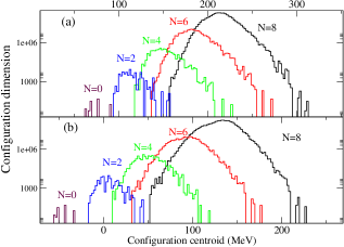
Figure 2: Evolution of configuration centroids for ¹²C under the similarity renormalization group, from $s=0$, or $\lambda=\infty$ (top panel) to $s=36.3\,\mathrm{GeV}^{-2}$ , or $\lambda=2.0\,\mathrm{fm}^{-1}$ (bottom panel). The abscissa is the configuration centroid, while the ordinate is the dimension of each configuration subspace. The two plots are shifted so their respective total centroids (3) are aligned. Here $N$ is the fixed number of excitations in harmonic oscillator many-body space, so that $N=4$ includes only 4 $\hbar\Omega$ excitation but no $0\hbar\Omega$, no $2\hbar\Omega$, etc. .

Fig. 2 plots the distribution of configurations centroids for ¹²C, both unevolved ($s=0$, top panel) and highly evolved (bottom panel) Hamiltonians, with the centroids combined into bins of width 2 MeV. The $y$-axis is the dimension of the binned configuration subspaces, on a log plot. The total centroid for each plot are aligned. Here $N$ is the number of excitations in the harmonic oscillator space. To be clear, here $N$ is fixed, not an upper limit; while CI calculations labeled by $N_{\mathrm{max}}$ include states with $N=N_{\mathrm{max}},N_{\mathrm{max}}-2,N_{\mathrm{max}}-4,\ldots$ ($\Delta N=2$ preserves parity), each curve in Fig. 2 is for all configurations of a single fixed $N$. Despite an overall shift of about 82 MeV in the centroids, the distribution of configuration centroids is remarkably unchanged. The main visible difference is the evolved configuration centroids are “stretched out.”

What about off-diagonal elements? Here I exploit another idea from SDT, that by using traces one can establish an inner product on operators [24]:

$$\left(\hat{H}_{1},\hat{H}_{2}\right)\equiv$$

$$\left\langle\left(\hat{H}_{1}-\langle\hat{H}_{1}\rangle^{({\cal S})}\right)\left(\hat{H}_{2}-\langle\hat{H}_{2}\rangle^{({\cal S})}\right)\right\rangle$$ (4)

$$=\langle\hat{H}_{1}\hat{H}_{2}\rangle^{({\cal S})}-\langle\hat{H}_{1}\rangle^{({\cal S})}\,\,\,\langle\hat{H}_{2}\rangle^{({\cal S})}.$$

With an inner product so defined, one has a metric on the space of Hamiltonians and can compare how close or distant two Hamiltonians are; the magnitude of a Hamiltonian, $\|\hat{H}\|=\sqrt{(\hat{H},\hat{H})}$, is its width, and the “angle” between two Hamiltonians by $\cos\theta=(\hat{H}_{1},\hat{H}_{2})\|\hat{H}_{1}\|^{-1}\|\hat{H}_{2}\|^{-1}$. Note that this definition of the metric is independent of the centroids, which is sensible as centroids affect only absolute energies and not excitation energies nor wave functions.

Using Eq. (1) and the cyclic property of traces,

$$\frac{d}{ds}\mathrm{tr}\,\hat{H}(s)\hat{G}=\mathrm{tr}\,[\hat{H}(s),\hat{G}]^{\dagger}[\hat{H}(s),\hat{G}].$$ (5)

But the righthand side is the trace of an operator of the form $\hat{A}^{\dagger}\hat{A}$, which manifestly has real and nonnegative eigenvalues and a real, nonnegative trace. Thus, under generic SRG, $\mathrm{tr}\,\hat{H}(s)\hat{G}$ can only increase; as the magnitudes of $\hat{H}(s)$ and, trivially, $\hat{G}$ are invariant, this means the “angle” defined by the inner product (4) between them can only get smaller and they become more and more parallel. Furthermore, this evolution stops when $[\hat{H}(s),\hat{G}]=0$, that is, the evolved Hamiltonian commutes with the generator. Thus SRG drives a Hamiltonian “towards” its generator. $\hat{H}(s)$ cannot become proportional to $\hat{G}$, as the eigenvalues, invariant under a unitary transformation, are different, but if one lets $s\rightarrow\infty$ they will have the same eigenvectors.

Interpretation using traces in the model space. Now let’s discuss these empirical results–the large, coherent shifts in low-lying energies, and the relatively modest changes in the wave function vectors–through the lens of spectral distribution theory, using traces as a fundamental tool to investigate what happens under the unitary transformation induced by SRG. To do so, one must pay attention to is the difference between taking traces in the full space and in the much smaller model space.

Let $\hat{H}$ be the original Hamiltonian in the full space, and let $\hat{H}^{\prime}=\hat{U}^{\dagger}\hat{H}\hat{U}$ be the transformed Hamiltonian. Since the full space is too large to work in, let the much smaller model space be ${\cal S}$ with a projection operator $\hat{P}_{\cal S}$.

The trace of any matrix (and of any power of that matrix) is preserved under unitary transformations: $\mathrm{tr}\,\hat{H}=\mathrm{tr}\,\hat{U}^{\dagger}\hat{H}\hat{U}=\mathrm{tr}\,\hat{H}^{\prime}$, and similarly $\mathrm{tr}\,\hat{H}^{2}=\mathrm{tr}\,(\hat{H}^{\prime})^{2}$. Let’s divide up the contributions to the trace of $\hat{H}^{2}$ into diagonal and off-diagonal pieces: $\mathrm{tr}\,\hat{H}^{2}=\sum_{i}H_{ii}^{2}+\sum_{i\neq j}H_{ij}^{2}$. If after a unitary transformation the matrix $\hat{H}^{\prime}$ is diagonal, then $\mathrm{tr}\,(\hat{H}^{\prime})^{2}$ has no off-diagonal contributions. Thus $\mathrm{tr}\,\hat{H}^{2}=\mathrm{tr}\,\hat{H}^{\prime 2}=\sum_{i}(H^{\prime})^{2}_{ii}\geq\sum_{i}H_{ii}^{2}$. That is, on average, the magnitude of the diagonal elements of the transformed matrix $\hat{H}^{\prime}$ must be larger than those of the original matrix $\hat{H}$.

Furthermore, the change in the diagonal matrix elements will generally be much larger than that of the off-diagonal matrix elements. How so? Even for sparse matrices, there will be many more off-diagonal matrix elements than diagonal. Suppose in an $N$-dimensional space there are $\sim N\times M$ non-zero off-diagonal matrix elements, so that $M/N\sim$ the sparsity. Further suppose the off-diagonal matrix elements all have roughly the same magnitude: call it $\gamma$. On average for every diagonal matrix element there are $\sim M$ non-zero matrix elements, and $\mathrm{tr}\,\hat{H}^{2}\sim\sum_{i}H_{ii}^{2}+NM\gamma^{2}$. Then on average $(H^{\prime}_{ii})^{2}\sim(H_{ii})^{2}+M\gamma^{2}$ so that the root-mean-square change in the diagonal matrix elements, $\delta H_{ii}\equiv\sqrt{(H^{\prime}_{ii})^{2}-(H_{ii})^{2}}\sim\sqrt{M}\,\gamma.$ Even for tiny sparsities, $M$ will be a large number. Hence the average changes of diagonal matrix elements will be substantially larger than the changes to the off-diagonal matrix elements.

This argument suggests that despite the large shift in the centroid in the model space, the changes to the off-diagonal matrix elements are much smaller. I argue this is true even when one is not fully diagonalizing but only applying a unitary transformation which “softens” the interaction. As further evidence, I use the metric introduced in Eq. (4). Fig. 3 graphically compares two Hamiltonian as the two vectors, with the magnitudes of each operator and the angle between them defined by (4), for four $p$-shell nuclides. I considered isospin zero many-body states; the results depend only weakly upon isospin. To focus on the actual evolution of the operators, I consider only the “interaction,” defined as $\hat{V}(s)=\hat{H}(s)-\hat{T}$, although such an interaction has components evolved from the original kinetic energy. The inner products were calculated using a publically available code [27]; because this code does not allow for $N_{\mathrm{max}}$ truncations, I instead truncated on the number of harmonic oscillator shells. I show the results for 7 major harmonic oscillator shells, that is, for maximum principal quantum number $N=6$, or up through the $3s$-$2d$-$1g$-$0i$ shell. The results, however, do not change very much as one goes from 5 to 7 major harmonic oscillator shells, and one can understand this as the higher excitations being nearly completely dominated by kinetic energy [28].

Fig. 3 shows the change in the interactions is modest. (Furthermore, although not included in Fig. 3, the angle between evolved and unevolved interactions in this space for $A=2,3$ is nearly identical to the cases shown.) This is in concordance with the previous empirical observation that under SRG evolution the change of the wave functions, as vectors in an abstract space of Slater determinants, is modest. Let me emphasize, however, that changes to the off-diagonal matrix elements are not negligible. If I approximate the SRG transformation by taking the unevolved Hamiltonian and simply swapping in the evolved configuration centroids, the shift in the ground state energy is overestimated by several MeV.

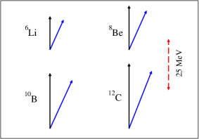
Figure 3: A representation of the evolution of interactions under SRG, as measured by the spectral distribution theory inner product, Eq. (4), for selected nuclides. The black, vertical arrows represent the unevolved interaction, at $s=0$ or $\lambda=\infty$, while the blue, tilted arrows are the interactions evolved to $s=36.3\,\mathrm{GeV}^{-2}$ or $\lambda=2.0\,\mathrm{fm}^{-1}$. Here the evolved interaction is defined as $\hat{V}(s)=\hat{H}(s)-\hat{T}$, where $\hat{T}$ is the kinetic energy. The red dashed line gives the scale. Although not shown, results for $A=2,3$ are very similar, although with smaller absolute magnitudes.

Eq. (5) proves that SRG evolves a Hamiltonian towards the generator. That proof, however, only applies in the full space. In the truncated model space, I find little change in the angle between the interaction and the kinetic energy, and in fact the angle increases, though by less than a degree.

Because the “full” Hamiltonian in the lab frame is generally far too large to be tractable, it must be truncated, which leads to loss of unitarity. But truncation is not the only cause of loss of unitarity. Three-body and higher-rank forces, induced by SRG [9, 18] also contribute to unitarity of the transformation. Previous work [29] as well as the success of the in-medium SRG [19, 20] has suggested the most important contributions of these many-body forces are those written as density- or state-dependent operators, especially those which contribute to the monopole terms [29], that is, the centroid and the configuration centroids. This is completely consistent with the results presented here.

Conclusions. Using traces or averages of operators in a many-body space, also called spectral distribution theory, is a powerful tool for understanding the evolution of nuclear forces under the similarity renormalization group. The primary effect of SRG is to simply to shift the model space centroid downwards. In contrast configuration centroids, or averages within occupancy-defined subspaces,are changed only a little relative to the total centroid. The inner product in SDT also allows one to look at off-diagonal matrix elements, which change only a modest amount under SRG. This picture–large, coherent shifts in the diagonal matrix elements and relatively much smaller changes to off-diagonal matrix elements–arises naturally when diagonalizing a Hamiltonian and is complementary to the conception of SRG “softening” the nuclear interaction. Finally, as the centroid and configuration centroids are written in terms of number operators, and the shift in the centroid is proportional to $A(A-1)$, I suggest one might compute separately the evolution of the centroid, not only as a function of $A(A-1)$ but also of higher powers of the number operator. Induced higher-particle-rank forces are important, and pieces proportional to powers of number operators account for the bulk of the effect [29].

I thank P. Navrǎtil for his code to generate the Entem-Machleidt N3LO force and apply SRG to it, and K. D. Launey for helpful discussions. This material is based upon work supported by the U.S. Department of Energy, Office of Science, Office of Nuclear Physics, under Award Number DE-FG02-03ER41272. This research used resources of the Argonne Leadership Computing Facility, which is a DOE Office of Science User Facility supported under Contract DE-AC02-06CH11357, and of the National Energy Research Scientific Computing Center, a DOE Office of Science User Facility supported by the Office of Science of the U.S. Department of Energy under Contract No. DE-AC02-05CH11231.

References

- Weinberg [1991] S. Weinberg, Nucl. Phys. B 363, 3 (1991).
- Van Kolck [1999] U. Van Kolck, Nuclear Physics A 645, 273 (1999).
- Machleidt and Entem [2011] R. Machleidt and D. R. Entem, Physics Reports 503, 1 (2011).
- Navrátil et al. [2000] P. Navrátil, J. Vary, and B. Barrett, Physical Review C 62, 054311 (2000).
- Barrett et al. [2013] B. R. Barrett, P. Navrátil, and J. P. Vary, Progress in Particle and Nuclear Physics 69, 131 (2013).
- Głazek and Wilson [1993] S. D. Głazek and K. G. Wilson, Phys. Rev. D 48, 5863 (1993).
- Wegner [1994] F. Wegner, Annalen der Physik 506, 77 (1994).
- Bogner et al. [2007] S. K. Bogner, R. J. Furnstahl, and R. J. Perry, Phys. Rev. C 75, 061001 (2007).
- Jurgenson et al. [2009] E. D. Jurgenson, P. Navrátil, and R. J. Furnstahl, Phys. Rev. Lett. 103, 082501 (2009).
- Bogner et al. [2010] S. Bogner, R. Furnstahl, and A. Schwenk, Progress in Particle and Nuclear Physics 65, 94 (2010).
- Stoks et al. [1994] V. Stoks, R. Klomp, C. Terheggen, and J. De Swart, Physical Review C 49, 2950 (1994).
- Wiringa et al. [1995] R. B. Wiringa, V. Stoks, and R. Schiavilla, Physical Review C 51, 38 (1995).
- Entem and Machleidt [2003] D. Entem and R. Machleidt, Physical Review C 68, 041001 (2003).
- Talmi et al. [1952] I. Talmi, R. Thieberger, K. Ford, E. Konopinski, M. Moshinsky, R. Lawson, M. Goeppert-Mayer, V. Balashov, V. Eltekov, A. Arima, et al., Helv. Phys. Acta 25, 185 (1952).
- Moshinsky [1959] M. Moshinsky, Nuclear Physics 13, 104 (1959).
- Brody and Moshinsky [1967] T. A. Brody and M. Moshinsky, (1967).
- Whitehead et al. [1977] R. R. Whitehead, A. Watt, B. J. Cole, and I. Morrison, Adv. Nuclear Phys. Vol. 9, pp 123-176 (1977).
- Launey et al. [2012] K. D. Launey, T. c. v. Dytrych, and J. P. Draayer, Phys. Rev. C 85, 044003 (2012).
- Tsukiyama et al. [2011] K. Tsukiyama, S. Bogner, and A. Schwenk, Physical review letters 106, 222502 (2011).
- Hergert et al. [2016] H. Hergert, S. Bogner, T. Morris, A. Schwenk, and K. Tsukiyama, Physics Reports 621, 165 (2016).
- Palumbo [1967] F. Palumbo, Nuclear Physics A 99, 100 (1967).
- Gloeckner and Lawson [1974] D. Gloeckner and R. Lawson, Physics Letters B 53, 313 (1974).
- Johnson et al. [2013] C. W. Johnson, W. E. Ormand, and P. G. Krastev, Computer Physics Communications 184, 2761 (2013).
- French [1967] J. B. French, Physics Letters B 26, 75 (1967).
- French [1983] J. B. French, Nuclear Physics A 396, 87 (1983).
- Wong [1986] S. S. M. Wong, Nuclear statistical spectroscopy, Vol. 7 (Oxford University Press, 1986).
- Launey et al. [2014] K. D. Launey, S. Sarbadhicary, T. Dytrych, and J. P. Draayer, Computer Physics Communications 185, 254 (2014).
- Shirokov et al. [2016] A. M. Shirokov, A. I. Mazur, I. A. Mazur, and J. P. Vary, Phys. Rev. C 94, 064320 (2016).
- Hagen et al. [2007] G. Hagen, T. Papenbrock, D. J. Dean, A. Schwenk, A. Nogga, M. Włoch, and P. Piecuch, Phys. Rev. C 76, 034302 (2007).