Strong Stability Preserving Integrating Factor Runge–Kutta Methods

Abstract. Strong stability preserving (SSP) Runge–Kutta methods are often desired when evolving in time problems that have two components that have very different time scales. Where the SSP property is needed, it has been shown that implicit and implicit-explicit methods have very restrictive time-steps and are therefore not efficient. For this reason, SSP integrating factor methods may offer an attractive alternative to traditional time-stepping methods for problems with a linear component that is stiff and a nonlinear component that is not. However, the strong stability properties of integrating factor Runge–Kutta methods have not been established. In this work we show that it is possible to define explicit integrating factor Runge–Kutta methods that preserve the desired strong stability properties satisfied by each of the two components when coupled with forward Euler time-stepping, or even given weaker conditions. We define sufficient conditions for an explicit integrating factor Runge–Kutta method to be SSP, namely that they are based on explicit SSP Runge–Kutta methods with non-decreasing abscissas. We find such methods of up to fourth order and up to ten stages, analyze their SSP coefficients, and prove their optimality in a few cases. We test these methods to demonstrate their convergence and to show that the SSP time-step predicted by the theory is generally sharp, and that the non-decreasing abscissa condition is needed in our test cases. Finally, we show that on typical total variation diminishing linear and nonlinear test-cases our new explicit SSP integrating factor Runge–Kutta methods out-perform the corresponding explicit SSP Runge–Kutta methods, implicit-explicit SSP Runge–Kutta methods, and some well-known exponential time differencing methods.

1 Introduction

When numerically solving a hyperbolic partial differential equation (PDE) of the form

$$U_{t}+f(U)_{x}=0,$$ (1)

the behavior of the numerical solution depends on properties of the spatial discretization combined with the time discretization. For smooth solutions, stability can be determined by analyzing the $L_{2}$ stability properties of the discretization applied to the linear problem. However, when dealing with a non-smooth solution, stability in the $L_{2}$ norm is not sufficient to ensure that the numerical solution will converge [52]. This is due to the presence of oscillations that prevents the approximation from converging uniformly. To ensure that the numerical method does not allow stability-destroying oscillations to form, we require that it satisfy stability properties in, e.g, the maximum norm or in the TV semi-norm.

Thus, to prove stability of numerical methods for nonlinear hyperbolic problems with discontinuous solutions, we need to analyze the nonlinear, non-inner-product stability properties of a highly nonlinear, complex spatial discretization combined with a high order time discretization. This is a difficult, sometimes untenable task. Instead, a method-of-lines formulation is generally followed, and a spatial discretization is developed that satisfies nonlinear, non-inner-product stability properties when coupled with the forward Euler time stepping method. In practice, higher order time discretizations are needed. Strong stability preserving (SSP) time-discretizations were created [68, 69] to allow the nonlinear non-inner product stability properties of the spatial discretizations coupled with forward Euler to be immediately extended to all SSP higher order time-discretizations.

1.1 Background

Linear stability theory is an indispensable tool used to establish the convergence of a numerical method when numerically solving PDEs. Linear stability is necessary and sufficient for convergence of a consistent linear numerical method when the PDE is linear [75]. When the PDE is nonlinear, if a numerical method is consistent and its linearization is $L_{2}$ stable and adequately dissipative, then convergence can be proved for sufficiently smooth problems [74]. However, discontinuous solutions often arise in the solution of hyperbolic conservation laws of the form (1), and when the solution has discontinuities, linear stability theory is no longer sufficient for convergence.

A famous example of this is that when the linearly $L_{2}$ stable second order Lax-Wendroff scheme is applied to Burgers’ equation, the method is nonlinearly unstable near stagnation points and does not converge [57]. This example demonstrates that to obtain convergence for a nonlinear PDE with a discontinuous solution, some kind of nonlinear stability is necessary in order to guarantee convergence.

Even in the linear case, $L_{2}$ stability is not enough for uniform convergence when dealing with solutions with discontinuities. For example, although a second order Lax-Wendroff scheme is strongly stable in the $L_{2}$ norm, when it is applied to a linear advection equation ($f(U)=aU$ in (1) above) with a step-function initial condition, the numerical solution will always have an overshoot or undershoot near the discontinuity [50]. Furthermore, this is true not only for the second order Lax-Wendroff but indeed any linear, consistent, finite difference scheme of at least second order accuracy will develop a an overshoot or undershoot that prevents uniform convergence [50].

These two examples show that $L_{2}$ linear stability is not the relevant property when we desire well-behaved numerical solutions of hyperbolic PDEs with discontinuous solutions. However, if we can prevent oscillations from forming by requiring stability in the maximum norm or the TV semi-norm, we can obtain uniform convergence [52]. Consequently, a tremendous amount of effort has been placed on the development of high order spatial discretizations which, when coupled with the forward Euler time stepping method, have the desired nonlinear stability properties for approximating discontinuous solutions of hyperbolic PDEs (see, e.g. [31, 61, 77, 13, 47, 78, 54]).

However, for actual computation, higher order time discretizations are usually needed. There is no guarantee that a spatial discretization that is strongly stable in some desired norm or semi-norm (e.g., $L_{\infty}$, or $TV$) for a nonlinear problem under forward Euler integration will possess the same nonlinear stability property when coupled with a linearly stable higher order time discretization. Strong stability preserving methods were created to address this need.

1.2 SSP methods

Explicit strong stability preserving (SSP) Runge–Kutta methods were first developed in [68, 69] for use in conjunction with total variation diminishing (TVD) spatial discretizations for hyperbolic conservation laws (1) with discontinuous solutions. These spatial discretizations of $f(U)_{x}$ ensure that when the resulting semi-discretized system of ordinary differential equations (ODEs)

$$u_{t}=F(u),$$ (2)

is evolved in time using the forward Euler method, a strong stability property

$$\|u^{n+1}\|=\|u^{n}+\Delta tF(u^{n})\|\leq\|u^{n}\|$$ (3)

is satisfied, under some step size restriction

$$0\leq\Delta t\leq\Delta t_{\textup{FE}}.$$ (4)

These TVD spatial discretizations are designed to satisfy the strong stability property

$$\|u^{n+1}\|\leq\|u^{n}\|$$ (5)

when coupled with the forward Euler time discretization. However, in actuality a higher order time integrator is desired, for both accuracy and linear stability reasons. If we can re-write a higher order time discretization as a convex combination of forward Euler steps, we can ensure that any convex functional property (5) that is satisfied by the forward Euler method will still be satisfied by the higher order time discretization, perhaps under a different time-step.

For example, we can write an $s$-stage explicit Runge–Kutta method in Shu-Osher form [28]:

$$u^{(0)} = u^{n},$$

$$u^{(i)} = \sum_{j=0}^{i-1}\left(\alpha_{i,j}u^{(j)}+\Delta t\beta_{i,j}F(u^{(j)})\right),\;\;\;\;i=1,...,s$$ (6)

$$u^{n+1} = u^{(s)}.$$

Note that for consistency, we must have $\sum_{j=0}^{i-1}\alpha_{i,j}=1$. If all the coefficients $\alpha_{i,j}$ and $\beta_{i,j}$ are non-negative, and a given $\alpha_{i,j}$ is zero only if its corresponding $\beta_{i,j}$ is zero, then each stage can be rearranged into a convex combination of forward Euler steps

$$\|u^{(i)}\|=\left\|\sum_{j=0}^{i-1}\left(\alpha_{i,j}u^{(j)}+\Delta t\beta_{i,j}F(u^{(j)})\right)\right\|\leq\sum_{j=0}^{i-1}\alpha_{i,j}\,\left\|u^{(j)}+\Delta t\frac{\beta_{i,j}}{\alpha_{i,j}}F(u^{(j})\right\|\leq\|u^{n}\|,$$

where the final inequality follows from (3) and (4) , provided that the time-step satisfies

$$\Delta t\leq\min_{i,j}\frac{\alpha_{i,j}}{\beta_{i,j}}\Delta t_{\textup{FE}}.$$ (7)

(Note that if any of the $\beta$’s are equal to zero, the corresponding ratio is considered infinite).

It is clear from this example that whenever we can re-write an explicit Runge–Kutta method as a convex combination of forward Euler steps, the forward Euler condition (3) will be preserved by the higher-order time discretizations, under the time-step restriction $\Delta t\leq\mathcal{C}\Delta t_{\textup{FE}}$ where $\mathcal{C}=\min_{i,j}\frac{\alpha_{i,j}}{\beta_{i,j}}$. As long as $\mathcal{C}>0$, the method is called strong stability preserving (SSP) with SSP coefficient $\mathcal{C}$ [68].

This form also ensures internal stage strong stability, i.e., $\|u^{(i+1)}\|\leq\|u^{(i)}\|$ at each stage $i$ of the time-stepping, under the same time-step restriction. The internal stage monotonicity property is important in simulations that involve pressure, density, or water height, in which a negative value even at the intermediate stage is not acceptable as it may not allow the simulation to proceed [32]. Positivity preserving limiters that prevent this from occurring are typically designed and proved for use with a forward Euler time-stepping and thus naturally extend to SSP time stepping methods with internal stage monotonicity [36, 87, 89, 90].

We observe that in the original papers [68, 69], the term $\|\cdot\|$ in Equation (3) above represented the total variation semi-norm. In general, though, the strong stability preservation property holds for any semi-norm, norm, or convex functional, as determined by the design of the spatial discretization. The only requirements are that the forward Euler condition (3) holds, and that the time-discretization can be decomposed into a convex combination of forward Euler steps with $\mathcal{C}>0$, as above.

Clearly, this convex combination condition is a sufficient condition for strong stability preservation. In fact, it has been shown that it is also necessary for strong stability preservation [28, 45, 72]. This means that if a method cannot be decomposed into a convex combination of forward Euler steps, then we can always find some ODE with some initial condition such that the forward Euler condition is satisfied but the method does not satisfy the strong stability condition for any positive time-step [28]. The observation that there are significant connections between SSP theory and contractivity theory [21, 22, 34, 35] has led to many results on SSP methods as well as development of new optimal and efficient SSP methods [23, 41, 40].

It is not always possible to decompose a method into convex combinations of forward Euler steps where $\mathcal{C}>0$. In fact in [45, 66] it was shown that explicit SSP Runge–Kutta methods cannot exist for order $p>4$. Furthermore, the value of $\mathcal{C}$ determines in large part what the size of an allowable time-step will be, and so we seek methods that have the largest possible SSP coefficient. Of course, a more important quantity is the total cost of the time evolution, which is related to the allowable time step relative to the number of function evaluations at each time-step. To allow us to compare the efficiency of explicit methods of a given order, we define the effective SSP coefficient $\mathcal{C}_{\textup{eff}}=\frac{\mathcal{C}}{s}$ where $s$ is the number of stages (typically the number of function evaluations). Unfortunately, all explicit $s$-stage Runge–Kutta methods have an SSP bound $\mathcal{C}\leq s$, and therefore $\mathcal{C}_{\textup{eff}}\leq 1$ [28]. Even worse, this upper bound is not usually attained. However, many efficient explicit SSP Runge–Kutta methods have been found, as we discuss in Section 2.

For smooth problems it is usually the case that implicit methods (or implicit treatment of stiff terms) can remove the time-step restriction needed for stability. In such cases, where the timestep is limited by a linear stability requirement or by an inner-product norm nonlinear stability there are well-known classes of implicit methods (e.g. A-stable, L-stable, B-stable) that allow the use of arbitrarily large timesteps. This is not the case for time discretizations of order $p>1$ where the time-step is limited by SSP considerations. For first order ($p=1$) it can be shown that if the spatial discretization is strongly stable in some norm under forward Euler time integration, then the fully discrete solution will also be strongly stable, in the same norm, for the implicit Euler method, without any timestep restriction [37, 34]. However, any general linear method of order $p>1$ can only be SSP under some finite timestep [71]. Worse yet, the timestep restrictions for implicit and implicit-explicit (IMEX) SSP methods are not dramatically larger than those for explicit methods, with the observed bound of $\mathcal{C}\leq 2s$, and therefore $\mathcal{C}_{\textup{eff}}\leq 2$ [51, 23, 41, 16].

SSP methods are widely used in the solution of hyperbolic PDEs, with discontinuous solutions, where linear $L_{2}$ stability is not enough to ensure convergence. They have been paired with many spatial discretizations that were specially designed for hyperbolic PDEs. Some of these spatial discretization approaches involve numerical methods that directly incorporate a non-oscillatory approach, such as ENO [9, 18, 3] and WENO [5, 10, 80, 20, 48, 4, 85, 62] methods, in a finite difference or finite element setting. These methods are typically designed and their properties proved with a forward Euler time-stepping, and rely on the SSP time-discretization mechanism to extend to higher order in time. Other approaches include limiters applied to finite difference or discontinuous Galerkin methods [14]. These limiters may enforce a total variation diminishing (TVD) [77] or total variation bounded (TVB) [67, 13] solution, or be used to ensure the numerical solution is maximum principle preserving [86, 88], or positivity preserving [87, 89, 90]. In these cases, SSP methods have proven particularly popular because for each new limiter proposed proofs of the desired property are generated for the method coupled with the first order forward Euler time-discretization. Once again, the SSP time-discretization mechanism is needed to extend the results on these limiters to higher order in time.

For spectral and pseudospectral methods, Reddy and Trefethen [65] explored the fact that eigenvalue stability is insufficient to ensure stable simulations, and discussed the difficulties in a fully-discrete stability analysis. Gottlieb and Tadmor [26] proved stability of spectral approximations for the forward Euler method; This is the approach commonly used in spectral methods simulations [33]. The work of Levy and Tadmor [53] shows the challenges of going from analysis of semi-discrete stability to fully discrete stability, as they analyzed the strong stability of Runge–Kutta schemes (including the first order forward Euler method) for linear problems. Gottlieb, Shu, and Tadmor later showed that the stability of the forward Euler method for any linear coercive approximations [53] could be easily extended using SSP analysis to a much larger class of Runge-Kutta methods. Furthermore, the SSP approach guarantees stability for much larger CFL numbers than the stability analysis in [53]. When using spectral methods on nonlinear problems, regularization using filtering [25, 33] or specially designed viscosity [56, 79, 55, 33] is needed for the simulation to be stable. The stabilization properties of these techniques are proven, usually, first on the semi-discrete form, and only then for the fully discrete form, in conjunction with a forward Euler step; the SSP time-stepping mechanism allows it to be preserved for higher order methods [33, 32].

In addition, SSP time-stepping methods have been paired with other spatial discretizations, including level set methods [64, 9, 19, 11, 15, 38], spectral finite volume methods [76, 12], and spectral difference methods [82, 83]. Examples of application areas where SSP time-stepping methods have been used include: compressible flow [82], incompressible flow [63], viscous flow [76], two-phase flow [9, 5], relativistic flow [18, 3, 85], cosmological hydrodynamics [20], magnetohydrodynamics [4], radiation hydrodynamics [58], two-species plasma flow [48], atmospheric transport [12], large-eddy simulation [62], Maxwell’s equations [14], semiconductor devices [10], lithotripsy [80], geometrical optics [15], and Schrodinger equations [11, 38].

1.3 SSP integrating factor Runge–Kutta methods

In this work, we are interested in a semi-discretized problem of the form

$$u_{t}=Lu+N(u)$$

where each component satisfies a forward Euler condition

$$\|u^{n}+\Delta tLu^{n}\|\leq\|u^{n}\|\;\;\;\mbox{for}\;\;\;\Delta t\leq\tilde{\Delta t_{\textup{FE}}}$$

and

$$\|u^{n}+\Delta tN(u^{n})\|\leq|\ u^{n}\|\;\;\;\mbox{for}\;\;\;\Delta t\leq{\Delta t_{\textup{FE}}},$$

(where $\|\cdot\|$ is some convex functional needed for non-linear, non-inner-product stability). In the cases of interest, $\tilde{\Delta t_{\textup{FE}}}<<{\Delta t_{\textup{FE}}}$, so that $L$ is a linear operator that significantly restricts the allowable time-step. As mentioned above, when the SSP properties are a concern, using an implicit-explicit (IMEX) scheme does not significantly alleviate the allowable time-step [16]. This motivates our investigation of integrating factor methods, where the linear component $Lu$ is handled exactly, and then the time-step restriction is, at worst, $\Delta t\leq{\Delta t_{\textup{FE}}}$ coming from the the nonlinear component $N(u)$. In this work, we discuss the conditions under which this process guarantees that the strong stability property (5) is preserved. In particular, we show that if we step the transformed problem forward using an SSP Runge–Kutta method where the abscissas (i.e. the time-levels approximated by each stage) are non-decreasing, we obtain a method that preserves the desired strong stability property. It is important to note that the efficient use of the proposed methods will depend heavily on the cost of computation of the matrix exponential. This area of research, although outside the scope of this work, will be crucial for the practical implementation of the SSP integrating factor Runge–Kutta methods described in this paper.

The paper is structured as follows: In Section 2 we review some known optimal and optimized explicit SSP Runge–Kutta methods of orders $p\leq 4$ and give the SSP coefficients and effective SSP coefficients of the optimal methods in this class. In Section 3 we describe explicit integrating factor (also known as Lawson type) Runge–Kutta (IFRK) methods [49]. We prove that when IFRK methods are based on explicit SSP Runge–Kutta methods with non-decreasing abscissas, they preserve the strong stability property. We also show an example that demonstrates that when using an IFRK method based on an explicit SSP Runge–Kutta method that has decreasing abscissas, the SSP property is violated. In Section 4 we formulate the optimization problem that will enable us to find optimized explicit SSP Runge–Kutta methods that have non-decreasing abscissas, and in Section 5 we present some optimized methods in this class and their SSP coefficients and effective SSP coefficients. We also prove the optimality of one of the methods in this class. In Section 6 we present numerical examples that show how our explicit SSP integrating factor Runge–Kutta (eSSPIFRK) methods perform on typical test cases compared to explicit, implicit-explicit (IMEX), and exponential time differencing (ETD) methods. We also compare the linear stability properties of these methods.

In Section 7 we conclude that the newly developed SSP theory for integrating factor Runge–Kutta methods provides a provable bound on the allowable time-step (which is often sharp in practice) for preservation of the nonlinear non-inner-product stability properties. Moreover, the newly developed methods demonstrate a significantly larger allowable SSP step-size than standard methods including the exponential time-differencing methods of Cox and Matthews [17], SSP IMEX methods [16], standard explicit SSP Runge–Kutta methods [28], as well as the Runge–Kutta methods of Kinnmark and Grey [44].

Note: The following acronyms and notations are used in this work:

IFRK	integrating factor Runge–Kutta method.
SSP	strong stability preserving.
eSSPRK	explicit SSP Runge–Kutta method.
eSSPRK+	explicit SSP Runge–Kutta method with non-decreasing abscissas.
eSSPKG	explicit SSP Kinnmark and Gray method.
eSSPRK+	explicit SSP Kinnmark and Gray method with
	non-decreasing abscissas.
eSSPIFRK	explicit SSP integrating factor Runge–Kutta method.
(s,p)	number of stages $s$ and order $p$.
IMEX	implicit-explicit additive method.
ETD	exponential time-differencing methods.

2 A review of explicit SSP Runge–Kutta methods

SSP Runge–Kutta methods guarantee the strong stability (in any norm, semi-norm, or convex functional) of the numerical solution of any ODE provided only that the forward Euler condition (3) is satisfied under a time step restriction (4). This requirement leads to severe restrictions on the allowable order of SSP methods, and the allowable time step $\Delta t\leq\mathcal{C}\Delta t_{\textup{FE}}.$ These methods have been extensively studied, e.g., in [21, 22, 23, 28, 29, 30, 34, 35, 37, 40, 41, 42, 43, 46, 66]. In this section, we review some popular and efficient explicit SSP Runge–Kutta methods, and present the SSP coefficients of optimized methods of up to ten stages and fourth order.

In the original papers on SSP time-stepping methods (there called TVD time-stepping) [68, 69], the authors presented the first explicit SSP Runge–Kutta methods. These methods were second and third order with SSP coefficient $\mathcal{C}=1$ ($\mathcal{C}_{\textup{eff}}=\frac{1}{2}$ and $\mathcal{C}_{\textup{eff}}=\frac{1}{3}$, respectively), and were proven optimal [29]. We use the notation eSSPRK(s,p) to denote an explicit SSP Runge–Kutta method with $s$ stages and of order $p$.

eSSPRK(2,2):

$$u^{(1)} = u^{n}+\Delta tF(u^{n})$$

$$u^{n+1} = \frac{1}{2}u^{n}+\frac{1}{2}\left(u^{(1)}+\Delta tF(u^{(1)})\right),$$ (8)

eSSPRK(3,3):

$$u^{(1)} = u^{n}+\Delta tF(u^{n})$$

$$u^{(2)} = \frac{3}{4}u^{n}+\frac{1}{4}\left(u^{(1)}+\Delta tF(u^{(1)})\right)$$

$$u^{n+1} = \frac{1}{3}u^{n}+\frac{2}{3}\left(u^{(2)}+\Delta tF(u^{(2)})\right).$$ (9)

Method (2) has been extensively used and is known as the Shu-Osher method.

No four stage fourth order explicit Runge–Kutta methods exist with a positive SSP coefficient [29, 66]. However, fourth order methods with more than four stages ($s>p$) do exist.

eSSPRK(5,4): Found by Spiteri and Ruuth [73]

$$u^{(1)} = u^{n}+0.391752226571890\Delta tF(u^{n})$$

$$u^{(2)} = 0.444370493651235u^{n}+0.555629506348765u^{(1)}+0.368410593050371\Delta tF(u^{(1)})$$

$$u^{(3)} = 0.620101851488403u^{n}+0.379898148511597u^{(2)}+0.251891774271694\Delta tF(u^{(2)})$$

$$u^{(4)} = 0.178079954393132u^{n}+0.821920045606868u^{(3)}+0.544974750228521\Delta tF(u^{(3)})$$

$$u^{n+1} = 0.517231671970585u^{(2)}+0.096059710526147u^{(3)}+0.063692468666290\Delta tF(u^{(3)})$$

$$+0.386708617503268u^{(4)}+0.226007483236906\Delta tF(u^{(4)})\,,$$

has $\mathcal{C}=1.508$ ($\mathcal{C}_{\textup{eff}}=0.302$).

eSSPRK(10,4): Found by Ketcheson [40], has a low-storage formulation:

$$u^{(1)} = u^{n}+\frac{1}{6}\Delta tF(u^{n})$$

$$u^{(i+1)} = u^{(i)}+\frac{1}{6}\Delta tF(u^{(i)})\;\;\;i=1,2,3$$

$$u^{(5)} = \frac{3}{5}u^{n}+\frac{2}{5}\left(u^{(4)}+\frac{1}{6}\Delta tF(u^{(4)})\right)$$

$$u^{(i+1)} = u^{(i)}+\frac{1}{6}\Delta tF(u^{(i)})\;\;\;i=5,6,7,8$$

$$u^{n+1} = \frac{1}{25}u^{n}+\frac{9}{25}\left(u^{(4)}+\frac{1}{6}\Delta tF(u^{(4)})\right)+\frac{3}{5}\left(u^{(9)}+\frac{1}{6}\Delta tF(u^{(9)})\right)\,,$$

has $\mathcal{C}=6$ ($\mathcal{C}_{\textup{eff}}=0.6$).

	2	3	4
1	-	-	-
2	1.0000	-	-
3	2.0000	1.0000	-
4	3.0000	2.0000	-
5	4.0000	2.6506	1.5082
6	5.0000	3.5184	2.2945
7	6.0000	4.2879	3.3209
8	7.0000	5.1071	4.1459
9	8.0000	6.0000	4.9142
10	9.0000	6.7853	6.0000

Table 1: SSP coefficients of the optimized eSSPRK(s,p) methods [28].

	2	3	4
1	-	-	-
2	0.5000	-	-
3	0.6667	0.3333	-
4	0.7500	0.5000	-
5	0.8000	0.5301	0.3016
6	0.8333	0.5864	0.3824
7	0.8571	0.6126	0.4744
8	0.8750	0.6384	0.5182
9	0.8889	0.6667	0.5460
10	0.9000	0.6785	0.6000

Table 2: Effective SSP coefficients of the optimized eSSPRK(s,p) methods [28].

In Table 2 we present the SSP coefficients of optimized explicit SSP Runge–Kutta methods of up to $s=10$ stages and order $p=4$, and in Table 2 the corresponding effective SSP coefficients. Unfortunately, no methods of order $p\geq 5$ with positive SSP coefficients can exist [45, 66].

3 Explicit SSP Runge–Kutta schemes for use with integrating factor methods

We consider a problem of the form

$$u_{t}=Lu+N(u)$$ (10)

with a linear constant coefficient component $Lu$ and a nonlinear component $N(u)$. The case we are interested in is when some strong stability condition is known for the forward Euler step of the nonlinear component $N(u)$

$$\|u^{n}+\Delta tN(u^{n})\|\leq\|u^{n}\|\qquad\mbox{for}\qquad\Delta t\leq\Delta t_{\textup{FE}}$$ (11)

while taking a forward Euler step using the linear component $Lu$ results in the strong stability condition

$$\|u^{n}+\Delta tLu^{n}\|\leq\|u^{n}\|\qquad\mbox{for}\qquad\Delta t\leq\tilde{\Delta t}_{\textup{FE}}$$ (12)

where $\tilde{\Delta t}_{\textup{FE}}<<\Delta t_{\textup{FE}}$. In such cases, stepping forward using an explicit SSP Runge–Kutta method, or even an implicit or an implicit-explicit (IMEX) SSP Runge–Kutta method will result in severe constraints on the allowable time-step [51, 41, 23, 28, 16].

An alternative methodology that may alleviate the restriction on the allowable time-step involves solving the linear part exactly using an integrating factor approach

$$e^{-Lt}u_{t}-e^{-Lt}Lu=e^{-Lt}N(u)$$

$$\left(e^{-Lt}u\right)_{t}=e^{-Lt}N(u).$$

A transformation of variables $w=e^{-Lt}u$ gives the ODE system

$$w_{t}=e^{-Lt}N(e^{Lt}w)=G(w),$$ (13)

which can then be evolved forward in time using, for example, an explicit Runge–Kutta method of the form (1.2). For each stage $u^{(i)}$, which corresponds to the solution at time $t_{i}=t^{n}+c_{i}\Delta t$ (where each $c_{i}$ is the abscissa of the method at the $i$th stage), the corresponding integrating factor Runge–Kutta method becomes

$$e^{-Lt_{i}}u^{(i)}=\sum_{j=0}^{i-1}\left(\alpha_{i,j}e^{-Lt_{j}}u^{(j)}+\Delta t\beta_{i,j}e^{-Lt_{j}}N(u^{(j)})\right),$$

or

$$u^{(i)} = \sum_{j=0}^{i-1}\left(\alpha_{i,j}e^{L(t_{i}-t_{j})}u^{(j)}+\Delta t\beta_{i,j}e^{L(t_{i}-t_{j})}N(u^{(j)})\right)$$

$$= \sum_{j=0}^{i-1}\left(\alpha_{i,j}e^{L(c_{i}-c_{j})\Delta t}u^{(j)}+\Delta t\beta_{i,j}e^{L(c_{i}-c_{j})\Delta t}N(u^{(j)})\right).$$

In the following results we establish the SSP properties of this approach.

Theorem 1.

If a linear operator $L$ satisfies (12) for some value of $\tilde{\Delta t}_{\textup{FE}}>0$, then

$$\|e^{\tau L}u^{n}\|\leq\|u^{n}\|\;\;\;\;\forall\;\tau\geq 0.$$ (14)

Proof.

The Taylor series expansion of $e^{z}$ can be written as

$$e^{z}=\sum_{j=0}^{\infty}\gamma_{j}(r)\left(1+\frac{z}{r}\right)^{j}\;\;\;\mbox{where}\;\;\gamma_{j}=\frac{r^{j}}{j!}e^{-r}$$

where the coefficients $\gamma_{j}$ are clearly nonnegative for all values of $r\geq 0$. These coefficients sum to one because

$$\sum_{j=0}^{\infty}\gamma_{j}=\sum_{j=0}^{\infty}\frac{r^{j}}{j!}e^{-r}=e^{-r}\sum_{j=0}^{\infty}\frac{r^{j}}{j!}=e^{-r}e^{r}=1.$$

Using this we can show that $e^{\tau L}u^{n}$ can be written as a convex combination of forward Euler steps with a modified time-step $\frac{\tau}{r}$, so that

$$\|e^{\tau L}u^{n}\| = \left\|\sum_{j=0}^{\infty}\gamma_{j}(r)\left(1+\frac{\tau}{r}L\right)^{j}u^{n}\right\|$$

$$\leq \sum_{j=0}^{\infty}\gamma_{j}(r)\left\|\left(1+\frac{\tau}{r}L\right)^{j}u^{n}\right\|$$

$$\leq \sum_{j=0}^{\infty}\gamma_{j}(r)\left\|u^{n}\right\|\leq\left\|u^{n}\right\|\;\;\mbox{for any $0\leq\tau\leq r\tilde{\Delta t}_{\textup{FE}}$}.$$

As this is true for any value of $r\geq 0$, we have

$$\|e^{\tau L}u^{n}\|\leq\|u^{n}\|\;\;\;\;\forall\tau\geq 0.$$

Note that a negative value of $\tau$ is not allowed here. ∎

Remark 1.

The thm above deals with the case that (12) is satisfied for some value of $\tilde{\Delta t}_{\textup{FE}}>0$. However, requiring $L$ to satisfy only condition (14) is sufficient for the integrating factor Runge–Kutta method to be SSP. In the following results, therefore, we only require the condition (14), which is a weaker condition than (12).

Corollary 1.

Given a linear operator $L$ that satisfies (14) and a (possibly nonlinear) operator $N(u)$ that satisfies (11) for some value of ${\Delta t}_{FE}>0$, we have

$$\|e^{\tau L}(u^{n}+\Delta tN(u^{n}))\|\leq\|u^{n}\|\;\;\;\;\forall\Delta t\leq\Delta t_{\textup{FE}},\;\;\;\mbox{provided that}\;\;\tau\geq 0.$$ (15)

Proof.

Separate the term $e^{\tau L}(u^{n}+\Delta tN(u^{n}))$ to two steps:

$$y^{(1)} = u^{n}+\Delta tN(u^{n})$$

$$y^{(2)} = e^{\tau L}y^{(1)}$$

Clearly, from (14) we have

$$\|y^{(2)}\|=\|e^{\tau L}y^{(1)}\|\leq\|y^{(1)}\|$$

for any $\tau\geq 0$. Now, from (11) we also have

$$\|y^{(1)}\|=\|u^{n}+\Delta tN(u^{n})\|\leq\|u^{n}\|\;\;\;\forall\Delta t\leq\Delta t_{\textup{FE}}.$$

Putting these two together we obtain the desired result. ∎

The following thm describes the conditions under which an integrating factor Runge–Kutta method is strong stability preserving.

Theorem 2.

Given a linear operator $L$ that satisfies (14) and a (possibly nonlinear) operator $N(u)$ that satisfies (11) for some value of ${\Delta t}_{FE}>0$, and a Runge–Kutta integrating factor method of the form

$$u^{(0)} = u^{n},$$

$$u^{(i)} = \sum_{j=0}^{i-1}e^{L(c_{i}-c_{j})\Delta t}\left(\alpha_{i,j}u^{(j)}+\Delta t\beta_{i,j}N(u^{(j)})\right),\;\;\;\;i=1,...,s$$ (16)

$$u^{n+1} = u^{(s)}$$

where $0=c_{1}\leq c_{2}\leq...\leq c_{s}$, then $u^{n+1}$ obtained from (2) satisfies

$$\|u^{n+1}\|\leq\|u^{n}\|\;\;\;\forall\Delta t\leq\mathcal{C}\Delta t_{\textup{FE}}.$$ (17)

Proof.

We observe that for each stage of (2)

$$\|u^{(i)}\| = \left\|\sum_{j=0}^{i-1}e^{L(c_{i}-c_{j})\Delta t}\left(\alpha_{i,j}u^{(j)}+\Delta t\beta_{i,j}N(u^{(j)})\right)\right\|$$

$$\leq \sum_{j=0}^{i-1}\left\|e^{L(c_{i}-c_{j})\Delta t}\left(\alpha_{i,j}u^{(j)}+\Delta t\beta_{i,j}N(u^{(j)})\right)\right\|$$

$$\leq \sum_{j=0}^{i-1}\alpha_{i,j}\left\|e^{L(c_{i}-c_{j})\Delta t}\left(u^{(j)}+\Delta t\frac{\beta_{i,j}}{\alpha_{i,j}}N(u^{(j)})\right)\right\|$$

where the last inequality follows from Corollary 1, as long as $c_{i}-c_{j}\geq 0$ and $\Delta t\frac{\beta_{i,j}}{\alpha_{i,j}}\leq\Delta t_{\textup{FE}}$. This establishes the result of the thm. Furthermore, this proof ensures that these methods have internal stage strong stability as well, i.e. $\|u^{(i+1)}\|\leq\|u^{(i)}\|$ at each stage $i$ of the time-stepping, under the same time-step restriction. ∎

Remark 2.

It is possible to preserve the strong stability property even with decreasing abscissas, provided that whenever the term $c_{i}-c_{j}$ is negative, the operator $L$ is replaced by an operator $\tilde{L}$ that satisfies the condition

$$\|e^{-\tau\tilde{L}}u^{n}\|\leq\|u^{n}\|\;\;\;\;\forall\;\tau\geq 0.$$

For hyperbolic partial differential equations, this is accomplished by using the spatial discretization that is stable for the downwinded analog of the operator. This approach is similar to the one employed in the classical SSP literature, where negative coefficients $\beta_{i,j}$ may be allowed if the corresponding operator is replaced by a downwinded operator [29, 30, 43].

Example: To demonstrate the practical importance of this thm, consider the partial differential equation

$$u_{t}+10u_{x}+\left(\frac{1}{2}u^{2}\right)_{x} =0\hskip 54.2025ptu(0,x)=\begin{cases}1,&\text{if }0\leq x\leq 1/2\\ 0,&\text{if }x>1/2\end{cases}$$

on the domain $[0,1]$ with periodic boundary conditions. We discretize the spatial grid with $400$ points and use a first-order upwind difference to semi-discretize the linear term $Lu\approx-10u_{x}$, and a fifth order WENO finite difference for the nonlinear terms $N(u)\approx-\left(\frac{1}{2}u^{2}\right)_{x}$. For the time discretization, we use the integrating factor method based on the explicit eSSPRK(3,3) Shu-Osher method (2):

$$u^{(1)} = e^{L\Delta t}u^{n}+e^{L\Delta t}\Delta tN(u^{n})$$

$$u^{(2)} = \frac{3}{4}e^{\frac{1}{2}L\Delta t}u^{n}+\frac{1}{4}e^{-\frac{1}{2}L\Delta t}u^{(1)}+\frac{1}{4}e^{-\frac{1}{2}L\Delta t}\Delta tN(u^{(1)})$$

$$u^{n+1} = \frac{1}{3}e^{L\Delta t}u^{n}+\frac{2}{3}e^{\frac{1}{2}L\Delta t}u^{(2)}+\frac{2}{3}e^{\frac{1}{2}L\Delta t}\Delta tN(u^{(2)}).$$ (18)

The appearance of exponentials with negative exponents is due to the fact that (2) has decreasing abscissas. For comparison we also use a IFRK(3,3) method based on an explicit SSP Runge–Kutta method with non-decreasing abscissas, denoted eSSPRK${}^{+}(3,3)$ (which will be presented in (3))

$$u^{(1)} = \frac{1}{2}e^{\frac{2}{3}\Delta tL}u^{n}+\frac{1}{2}e^{\frac{2}{3}\Delta tL}\left(u^{n}+\frac{4}{3}\Delta tN(u^{n})\right)$$

$$u^{(2)} = \frac{2}{3}e^{\frac{2}{3}\Delta tL}u^{n}+\frac{1}{3}\left(u^{(1)}+\frac{4}{3}\Delta tN(u^{(1)})\right)$$

$$u^{n+1} = \frac{59}{128}e^{\Delta tL}u^{n}+\frac{15}{128}e^{\Delta tL}\left(u^{n}+\frac{4}{3}\Delta tN(u^{n})\right)$$

$$+\frac{27}{64}e^{\frac{1}{3}\Delta tL}\left(u^{(2)}+\frac{4}{3}\Delta tN(u^{(2)})\right).$$

The eSSPRK${}^{+}(3,3)$ method this integrating factor is based on has SSP coefficient $\mathcal{C}=\frac{3}{4}$, which is smaller than the $\mathcal{C}=1$ of the Shu-Osher method (2), due to the restriction on the non-decreasing abscissas. thm 2 above tells us that the IFRK method (3) will be SSP while the IFRK method (3) based on the Shu-Osher method (2) will not be.

We selected different values of $\Delta t$ and used each one to evolve the solution 25 time steps using the IFRK methods (3) and (3). We calculated the maximal rise in total variation over each stage for 25 time steps. In Figure 1 we show the $log_{10}$ of the maximal rise in total variation vs. the value of $\lambda=\frac{\Delta t}{\Delta x}$ of the evolution using (3) (in blue) and using (3) (in red). We observe that the results from method (3) have a large maximal rise in total variation even for very small values of $\lambda$, while the results from (3) maintain a small maximal rise in total variation up to $\lambda\approx 0.8$.

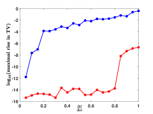
Figure 1: Total variation behavior of the evolution over 25 time-steps using the integrating factor methods (3) (blue dots) and (3) (red stars).

This example clearly illustrates that basing an IFRK method on an explicit SSP Runge–Kutta method is not enough to ensure the preservation of a strong stability property. In this case, we must use the non-decreasing abscissa condition in thm (2) to ensure that the strong stability property is preserved.

4 Formulating the optimization problem

Our aim is to find eSSPRK(s,p) methods to evolve an equation of the form (2) which have non-decreasing abscissas and largest SSP coefficient $\mathcal{C}$. We denote these methods eSSPRK⁺(s,p). These methods can then be used to produce an integrating factor method (2) that has a guarantee of nonlinear stability, as we showed in Section 3 above. Following the approach developed by Ketcheson [40], we formulate an optimization problem similar to the one used for explicit SSP Runge-Kutta methods [28] but with one additional constraint.

Although the SSP coefficient $\mathcal{C}$ is most easily seen in Shu-Osher form, constructing the optimization problem is easier when the method is written in Butcher form:

$$u^{(i)} = u^{n}+\Delta t\sum_{j=1}^{i-1}a_{ij}F(u^{(j)})\;\;\;\;(1\leq i\leq s)$$ (20)

$$u^{n+1} = u^{n}+\Delta t\sum_{j=1}^{s}b_{j}F(u^{(j)}).$$

We can put all the $a_{ij}$ values into a matrix $\mathbf{A}$ and all the $b_{j}$ into a vector $\mathbf{b}$. Then we define the vector of abscissas $\mathbf{c}=\mathbf{A}\mathbf{e}$, where $\mathbf{e}$ is the vector of ones of the appropriate length. We rewrite (20) in vector form

$$Y=\mathbf{e}u^{n}+\Delta t\mathbf{S}F(Y)$$

where $\mathbf{S}$ is the square matrix defined by:

$$\mathbf{S}=\left(\begin{array}[]{ll}\mathbf{A}&0\\ \mathbf{b}^{T}&0\\ \end{array}\right).$$

We add $r\mathbf{S}Y$ to each side to obtain

$$\left(I+r\mathbf{S}\right)Y=\mathbf{e}u^{n}+r\mathbf{S}\left(Y+\frac{\Delta t}{r}F(Y)\right)\quad\Rightarrow\quad Y=\mathbf{R}(\mathbf{e}u^{n})+\mathbf{P}\left(Y+\frac{\Delta t}{r}F(Y)\right),$$

for $\mathbf{R}=\left(I+r\mathbf{S}\right)^{-1}$ and $\mathbf{P}=r\mathbf{R}\mathbf{S}.$ Clearly, if $\mathbf{R}\mathbf{e}$ and $\mathbf{P}$ have all non-negative components, we have a convex combination of forward Euler steps. Therefore, the strong stability property (5) will be preserved under the modified time-step restriction $\Delta t\leq r\Delta t_{\textup{FE}}$.

As discussed in [28], the goal is to maximize the value of $r$ subject to the constraints

$$\left(I+r\mathbf{S}\right)^{-1}\mathbf{e}\geq 0$$ (21a)

$$r\left(I+r\mathbf{S}\right)^{-1}\mathbf{S}\geq 0$$ (21b)

$$\tau_{k}(\mathbf{A},\mathbf{b})=0\;\;\;\mbox{for}\;\;\;k=1,...,P,$$ (21c)

Where in the inequalities are all component wise and $$\tau_{k}$$ in (21c) are the order conditions.

In addition to the constraints (21a) – (21c), we must also add the condition that the abscissas are non-decreasing

$$c_{1}\leq c_{2}\leq\dots\leq c_{s}\leq 1.$$ (21d)

Solving this optimization problem will generate an explicit SSP Runge–Kutta method with coefficients $\mathbf{A}$ and $\mathbf{b}$ such that the abscissas are non-decreasing, with a SSP coefficient $\mathcal{C}=r$.

4.1 Order conditions

The equality constraints (21c) for the optimization problem above come from the order conditions, which were derived in [8]. Below are the order conditions for methods up to fourth order. For first order a method must satisfy the consistency condition:

$$\mathbf{b}^{T}\mathbf{e} =1.$$

In addition to this condition second order methods must also satisfy:

$$\mathbf{b}^{T}\mathbf{c} =\frac{1}{2}.$$

There are two more order conditions required to obtain third order:

$$\mathbf{b}^{T}\left(\mathbf{c}\cdot\mathbf{c}\right) =\frac{1}{3}, \mathbf{b}^{T}\mathbf{A}\mathbf{c}=\frac{1}{6}.$$

For fourth order four additional conditions must be satisfied:

$$\mathbf{b}^{T}\left(\mathbf{c}\cdot\mathbf{c}\cdot\mathbf{c}\right)=\frac{1}{4},\;\;\;\mathbf{b}^{T}\left(\mathbf{c}\cdot\mathbf{A}\mathbf{c}\right)=\frac{1}{8},\;\;\;\mathbf{b}^{T}\mathbf{A}\left(\mathbf{c}\cdot\mathbf{c}\right)=\frac{1}{12},\;\;\;\mathbf{b}^{T}\mathbf{A}^{2}\mathbf{c}=\frac{1}{24}.\;\;\;$$

Note that $(\mathbf{a}\cdot\mathbf{b})$ denotes element-wise multiplication. We do not present the order conditions past fourth order since there are no explicit SSP Runge–Kutta methods greater than fourth order.

5 Optimal and optimized methods

The optimization problem above was implemented in Matlab (as in [40, 42, 41]), and used to find optimized eSSPRK⁺ methods of up to ten stages and fourth order. These methods have non-decreasing abscissas and so can be used as a basis for explicit SSP integrating factor Runge–Kutta (eSSPIFRK) methods.

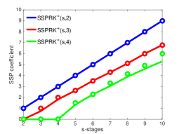
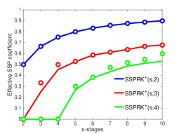
Figure 2: SSP coefficient (left) and effective SSP coefficient (right) for orders for $p=2$ (blue), $p=3$ (red) and $p=4$ (green) methods. The circles indicate the SSP coefficient of the optimized eSSPRK methods while the lines are the SSP coefficients of the optimized eSSPRK⁺ methods.

The SSP coefficients and effective SSP coefficients of the optimized eSSPRK⁺ methods are listed in Tables 4 and 4. The SSP coefficients of this family of methods are compared to those of the optimized eSSPRK methods with no constraint on the abscissas in Figure 2, where the circles indicate the SSP coefficient of the optimized explicit SSPRK methods while the lines are the SSP coefficients of the optimized explicit SSPRK⁺ methods.

We observe that the optimal second order methods we found have the same SSP coefficients as the previously known SSP Runge–Kutta methods. This is not surprising as the abscissas of those optimal methods are non-decreasing, so our optimization routine found the previously known optimal methods. These eSSPRK⁺(s,2) methods have SSP coefficient $\mathcal{C}=s-1$ and effective SSP coefficient $\mathcal{C}_{\textup{eff}}=\frac{s-1}{s}$. In Section 5.2 we give the coefficients for these methods in both Shu-Osher form and Butcher form and show that the abscissas are indeed non-decreasing.

In the third order case, the additional requirement that the abscissas be non-decreasing results in smaller SSP coefficients than the typical explicit SSP Runge–Kutta methods. For example, the optimal eSSPRK(3,3) Shu-Osher method (2) has SSP coefficient $\mathcal{C}=1$ while the optimal eSSPRK⁺(3,3) method has SSP coefficient $\mathcal{C}=\frac{3}{4}$, as we will prove in Section 5.3. This loss in the SSP coefficient is also evident for the eSSPRK⁺(4,3) method ($\mathcal{C}=\frac{20}{11}$) compared to the eSSPRK(4,3) method ($\mathcal{C}=2$). However, as we add more stages the impact of the additional requirement of non-decreasing abscissas becomes negligible and the SSP coefficients of the eSSPRK⁺(s,3) methods are very close to those of the standard eSSPRK(s,3) methods, as seen in Figure 2.

	2	3	4
1	-	-	-
2	1.0000	-	-
3	2.0000	0.7500	-
4	3.0000	1.8182	-
5	4.0000	2.6351	1.3466
6	5.0000	3.5184	2.2738
7	6.0000	4.2857	3.0404
8	7.0000	5.1071	3.8926
9	8.0000	6.0000	4.6048
10	9.0000	6.7853	5.2997

Table 3: SSP coefficients of the optimized eSSPRK⁺(s,p) methods.

	2	3	4
1	-	-	-
2	0.5000	-	-
3	0.6667	0.2500	-
4	0.7500	0.4545	-
5	0.8000	0.5270	0.2693
6	0.8333	0.5864	0.3790
7	0.8571	0.6122	0.4343
8	0.8750	0.6384	0.4866
9	0.8889	0.6667	0.5116
10	0.9000	0.6785	0.5300

Table 4: Effective SSP coefficients of the optimized eSSPRK⁺(s,p) methods..

In the fourth order case, the SSP coefficient of the optimized eSSPRK⁺ are certainly smaller than those of the corresponding eSSPRK methods. In fact, this does not significantly improve as we increase the number of stages. Notably, the optimal eSSPRK(10,4) method found by Ketcheson [40] has an SSP coefficient of $\mathcal{C}=6$ while the corresponding eSSPRK⁺(10,4) method has SSP coefficient $\mathcal{C}=5.3$, a reduction of over 10%. An exception to this is the optimized eSSPRK⁺(6,4) method in which the non-descreasing abscissa requirement results in only a $1\%$ reduction of the SSP coefficient compared to the eSSPRK(6,4).

5.1 Sub-optimal explicit SSP Kinnmark and Gray Runge–Kutta methods with non-decreasing abscissas

In [44], Kinnmark and Gray presented a set of Runge–Kutta methods for linear problems. More precisely, they presented the linear stability polynomials for these methods. These methods were designed for use with problems that require a linear stability polynomials that include a large area of the imaginary axis. It is interesting to investigate what types of SSP coefficients the methods described in [44] can have. To do so, we modified our code that finds SSP Runge–Kutta methods of $s$ stages and order $p$ to include the linear stability polynomials of Kinnmark and Gray and used this code to find optimized SSP methods with $(s,p)=(3,3),(5,3),(6,4)$. We call these eSSPKG(s,p) methods and present their SSP coefficients and a comparison to the corresponding eSSPRK(s,p) methods in Table 5. All explicit SSP Runge–Kutta methods of $s=p=3$ have the same stability polynomial, so that the Kinnmark and Gray methods eSSPKG(3,3) have the same linear stability region as eSSPRK(3,3). Although the SSP coefficients of the other SSP Kinnmark and Gray methods are smaller than those of the typical SSP Runge–Kutta methods, they may be used if the linear stability regions of Kinnmark and Gray are of interest. Note that the approach of optimizing an SSP method for a given linear stability region was originally done by [46]. For comparison, we provide the linear stability regions in Figure 3. We observed that, as expected, the Kinnmark Gray methods have larger imaginary axis stability, but smaller overall regions.

Next, we added the requirement that the abscissas are non-decreasing to find optimized SSPKG+(s,p) methods for $(s,p)=(3,3),(5,3),(6,4)$, and compare their SSP coefficients to those of the SSPRK+(s,p), also in Table 5. These methods are suitable for use with Lawson-type integrating factor methods. In Figure 3 we show the linear stability regions of the $(s,p)=(5,3)$ and $(s,p)=(6,4)$ methods, as well. We test the SSPKG methods as well as their use within the integrating factor approach in Example 3, where we see that their allowable time-step for preserving the TVD properties of a simple benchmark method are generally smaller than those of the SSPRK+ methods and the SSPRKIF methods.

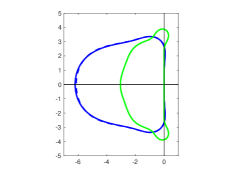
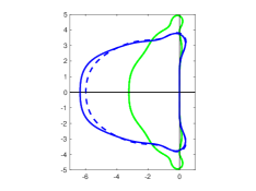
Figure 3: Linear stability region of the Kinnmark and Gray methods (in green) compared to the eSSPRK method (blue solid line) and the eSSPRK+ method (blue dashed line). Left: method with $(s,p)=(5,3)$; Right: method with $(s,p)=(6,4)$.

method	$\mathcal{C}$	method	$\mathcal{C}$
eSSPRK(5,3)	2.6506	eSSPRK+(5,3)	2.6351
eSSPKG(5,3)	1.0000	eSSPKG+(5,3)	0.8750
eSSPRK(6,4)	2.2945	eSSPRK+(6,4)	2.2738
eSSPKG(6,4)	0.9904	eSSPKG+(6,4)	0.7851

Table 5: SSP coefficients of the optimized SSP Runge–Kutta methods designed for the Kinnmark and Gray stability regions (eSSPKG methods, in bold) compared to typical SSP Runge–Kutta methods (eSSPRK methods), with (right column) and without (left column) non-decending abscissas.

5.2 Optimal second order explicit SSP Runge–Kutta methods with non-decreasing abscissas

We mentioned above that the optimal eSSPRK(s,2) methods have non-decreasing coefficients. In this section we review these methods, first presented in [30], and show that the abscissas are in fact increasing. These methods can be written in Shu-Osher form (where $u^{(0)}=u^{n}$) :

$$\begin{split}u^{(i)}&=u^{(i-1)}+\frac{\Delta t}{s-1}F(u^{(i-1)}),\quad i=1,\dots,s-1\\ u^{(s)}&=\frac{1}{s}u^{0}+\frac{s-1}{s}\left(u^{(s-1)}+\frac{\Delta t}{s-1}F(u^{(s-1)})\right)\\ u^{n+1}&=u^{(s)}.\end{split}$$

In Butcher form, this becomes

$$\mathbf{A}=\begin{bmatrix}0&0&0&\dots&0&0\\ \frac{1}{s-1}&0&0&\dots&0&0\\ \frac{1}{s-1}&\frac{1}{s-1}&0&\dots&0&0\\ \vdots&\ddots&\ddots&\ddots&\vdots&\vdots\\ \frac{1}{s-1}&\frac{1}{s-1}&\frac{1}{s-1}&\frac{1}{s-1}&0&0\\ \frac{1}{s-1}&\frac{1}{s-1}&\frac{1}{s-1}&\frac{1}{s-1}&\frac{1}{s-1}&0\end{bmatrix},\;\;\mathbf{b}^{T}=\begin{bmatrix}\frac{1}{s}\\ \frac{1}{s}\\ \frac{1}{s}\\ \vdots\\ \frac{1}{s}\\ \frac{1}{s}\\ \end{bmatrix}\;,$$

with abscissas

$$\mathbf{c}^{T}=\left[0,\frac{1}{s-1},\frac{2}{s-1},\dots\frac{s-2}{s-1},1\right].$$

Clearly, these optimal explicit SSP Runge–Kutta methods have increasing abscissas, and are therefore suitable use with an integrating factor approach to create eSSPIFRK methods.

5.3 Optimized third order explicit SSP Runge–Kutta methods with non-decreasing abscissas

Theorem 3.

The eSSPRK⁺(3,3) method given by

$$u^{(1)} = \frac{1}{2}u^{n}+\frac{1}{2}\left(u^{n}+\frac{4}{3}\Delta tF(u^{n})\right)$$

$$u^{(2)} = \frac{2}{3}u^{n}+\frac{1}{3}\left(u^{(1)}+\frac{4}{3}\Delta tF(u^{(1)})\right)$$

$$u^{n+1} = \frac{59}{128}u^{n}+\frac{15}{128}\left(u^{(1)}+\frac{4}{3}\Delta tF(u^{(1)})\right)+\frac{27}{64}\left(u^{(2)}+\frac{4}{3}\Delta tF(u^{(2)})\right).$$ (22)

is strong stability preserving with SSP coefficient $\mathcal{C}=\frac{3}{4}$ and is optimal among all eSSPRK⁺(3,3) methods.

Proof.

This method is given in its canonical Shu-Osher form. Clearly, we have a convex combination of forward Euler steps with time-step $\frac{4}{3}\Delta t$ and so this method is SSP with $\mathcal{C}=\frac{3}{4}$.

To show that this is optimal among all possible eSSPRK⁺(3,3) methods, we follow along the lines of the proof in [28]. We assume that $\mathcal{C}>\frac{3}{4}$, which means that $\frac{\alpha_{ij}}{\beta_{ij}}>\frac{3}{4}$ or

$$\alpha_{ij}>\frac{3}{4}\beta_{ij}\quad\mbox{for any}\quad i,j,$$

and proceed with a proof by contradiction.

First, recall that we can transform between the Shu-Osher coefficients $\alpha,\beta$ and the Butcher array coefficients $\mathbf{A}$ and $\mathbf{b}$ as follows:

$$\begin{split}a_{21}=&\beta_{10},\;\;a_{31}=\beta_{20}+\alpha_{21}\beta_{10},\;\;a_{32}=\beta_{21}\\ b_{1}=&\alpha_{32}\alpha_{21}\beta_{10}+\alpha_{31}\beta_{10}+\alpha_{32}\beta_{20}+\beta_{30},\;\;b_{2}=\alpha_{32}\beta_{21}+\beta_{31},\;\;b_{3}=\beta_{32}\\ c_{1}=&0,\;\;c_{2}=a_{21},\;\;c_{3}=a_{31}+a_{32}.\\ \end{split}$$

Note that for the method to be SSP, the coefficients must all be non-negative. If the abscissas are non-decreasing, there are two possible cases: $c_{2}=c_{3}$ and $c_{2}<c_{3}$. We consider each of these cases separately.

[Case (a)] If the abscissas are equal, they must be $c_{2}=c_{3}=\frac{2}{3}$. The coefficients in this case satisfy

$$a_{21}=\frac{2}{3},\;\;a_{31}=\frac{2}{3}-\frac{1}{4\omega},\;\;a_{32}=\frac{1}{4\omega},\;\;b_{1}=\frac{1}{4},\;\;b_{2}=\frac{3}{4}-\omega,\;\;b_{3}=\omega$$

for parameter $\omega$. The assumption that $\alpha_{ij}>\frac{3}{4}\beta_{ij}$ and the non-negativity assumption on the coefficients results in

$$b_{2}=\alpha_{32}\beta_{21}+\beta_{31}\geq\alpha_{32}\beta_{21}>\frac{3}{4}\beta_{32}\beta_{21}=\frac{3}{4}b_{3}a_{32}=\frac{3}{16}\implies\omega<\frac{9}{16}.$$

On the other hand,

$$a_{31}=\beta_{20}+\alpha_{21}\beta_{10}\geq\alpha_{21}\beta_{10}>\frac{3}{4}\beta_{21}\beta_{10}=\frac{3}{4}a_{32}a_{21}=\frac{3}{4}\frac{1}{4\omega}\frac{2}{3}=\frac{1}{8\omega}$$

so that

$$\frac{2}{3}-\frac{1}{4\omega}>\frac{1}{8\omega}\implies\omega>\frac{9}{16},$$

which contradicts the bound on $\omega$ above.

[Case (b)] If the two abscissas are not equal, and we require non-decreasing abscissas, we must have $c_{2}<c_{3}$. In this case, the coefficients are given by a two parameter system, where the parameters are the abscissas $c_{2}$ and $c_{3}$.

$$a_{21}=c_{2},\;\;a_{31}=\frac{3c_{2}c_{3}(1-c_{2})-c_{3}^{2}}{c_{2}(2-3c_{2})},\;\;a_{32}=\frac{c_{3}(c_{3}-c_{2})}{c_{2}(2-3c_{2})}$$

$$b_{1}=1+\frac{2-3(c_{2}+c_{3})}{6c_{2}c_{3}},\;\;b_{2}=\frac{3c_{3}-2}{6c_{2}(c_{3}-c_{2})},\;\;b_{3}=\frac{2-3c_{2}}{6c_{3}(c_{3}-c_{2})}.$$

The requirement that $c_{2}<c_{3}$ and that both $b_{2}$ and $b_{3}$ are non-negative gives

$$\begin{split}b_{2}=&\frac{3c_{3}-2}{6c_{2}(c_{3}-c_{2})}\geq 0\implies c_{3}\geq\frac{2}{3}\\ b_{3}=&\frac{2-3c_{2}}{6c_{3}(c_{3}-c_{2})}\geq 0\implies c_{2}\leq\frac{2}{3}.\\ \end{split}$$

Now begin with $a_{31}=\beta_{20}+\alpha_{21}\beta_{10}$, and recall that $\alpha_{21}>\frac{3}{4}\beta_{21}$ and $\beta_{10}=a_{21}=c_{2}$ and $\beta_{21}=a_{32}$, so that

$$a_{31}>\frac{3}{4}\beta_{21}c_{2}=\frac{3}{4}a_{32}c_{2}\implies c_{3}-a_{32}>\frac{3}{4}a_{32}c_{2}\implies c_{3}>a_{32}\left(1+\frac{3}{4}c_{2}\right)$$

which requires $a_{32}<\frac{c_{3}}{\left(1+\frac{3}{4}c_{2}\right)}$.

Using the definition of $a_{32}$, this means

$$\frac{c_{3}(c_{3}-c_{2})}{c_{2}(2-3c_{2})}<\frac{c_{3}}{\left(1+\frac{3}{4}c_{2}\right)}\implies c_{3}<\frac{3c_{2}-\frac{9}{4}c_{2}^{2}}{\left(1+\frac{3}{4}c_{2}\right)}.$$

Next, we look use the fact that $\beta_{31}\geq 0$ to obtain

$$b_{2}=\alpha_{32}\beta_{21}+\beta_{31}\geq\alpha_{32}\beta_{21}>\frac{3}{4}b_{3}a_{32}\implies a_{32}<\frac{4}{3}\frac{b_{2}}{b_{3}}=\frac{4}{3}\frac{c_{3}(3c_{3}-2)}{c_{2}(2-3c_{2})}.$$

Now we use $a_{32}=\frac{c_{3}(c_{3}-c_{2})}{c_{2}(2-3c_{2})}$ to conclude that

$$\frac{c_{3}(c_{3}-c_{2})}{c_{2}(2-3c_{2})}<\frac{4}{3}\frac{c_{3}(3c_{3}-2)}{c_{2}(2-3c_{2})}\implies c_{3}>-\frac{1}{3}c_{2}+\frac{8}{9}.$$

We now have two statements that need to be simultaneously true

$$c_{3}<\frac{3c_{2}-\frac{9}{4}c_{2}^{2}}{\left(1+\frac{3}{4}c_{2}\right)}\;\;\mbox{and}\;\;c_{3}>-\frac{1}{3}c_{2}+\frac{8}{9}$$

which means that we must have

$$-\frac{1}{3}c_{2}+\frac{8}{9}<\frac{3c_{2}-\frac{9}{4}c_{2}^{2}}{\left(1+\frac{3}{4}c_{2}\right)}\implies(3c_{2}-2)^{2}<0$$

however this is a contradiction because $(3c_{2}-2)^{2}$ is always greater than or equal to zero. This means that our original assumption was not correct, and that if $c_{2}<c_{3}$ we cannot have $\mathcal{C}>\frac{3}{4}$. ∎

5.4 Recommended SSP Runge–Kutta methods for use with integrating factor methods

The optimal second order methods eSSPRK⁺(s,2) listed above have sparse Shu-Osher representations and a general formula. However, for the optimized third and fourth order methods, we do not have a general formula. In this section we list a few of the optimized third and fourth order methods. The coefficients of all the methods we found can be downloaded as .mat files from our github repository [27].

eSSPRK⁺(4,3) This method has rational coefficients and sparse Shu-Osher matrices:

$$u^{(1)} = u^{n}+\frac{11}{20}\Delta tF(u^{n})$$

$$u^{(2)} = \frac{3}{8}u^{n}+\frac{5}{8}\left(u^{(1)}+\frac{11}{20}\Delta tF(u^{(1)})\right)$$

$$u^{(3)} = \frac{4}{9}u^{n}+\frac{5}{9}\left(u^{(2)}+\frac{11}{20}\Delta tF(u^{(2)})\right)$$

$$u^{n+1} = \frac{111}{1331}u^{n}+\frac{260}{1331}\left(u^{n}+\frac{11}{20}\Delta tF(u^{n})\right)+\frac{960}{1331}\left(u^{(3)}+\frac{11}{20}\Delta tF(u^{(3)})\right)$$

The abscissas are $c_{1}=0,c_{2}=\frac{11}{20},c_{3}=c_{4}=\frac{11}{16}$. This method has $\mathcal{C}=\frac{20}{11}$.

When many stages are required for a high order computation, the amount of storage, particularly for large simulations, may become prohibitive. Low storage methods are of great interest in such cases. Low storage Runge–Kutta methods were considered in [84, 39, 81]. More recently, Ketcheson [40] developed many low-storage SSP methods and showed that some of the most efficient methods in terms of the SSP coefficient are also efficient in terms of storage. This method is low-storage in the sense of [40], as many of the storage registers can be overwritten during the implementation, assuming one is willing to recompute $F(u^{i})$ when needed [40, 28]. Due to the structure of the Shu-Osher matrices, only two memory registers are required for this method, rather than the full $s+1=5$ that would be needed for a naive implementation.

eSSPRK⁺(9,3) This method has $\mathcal{C}=6$ and features rational coefficients and sparse Shu-Osher matrices:

$$\begin{split}u^{(0)}=&u^{n}\\ u^{(i)}=&u^{(i-1)}+\frac{1}{6}\Delta tF(u^{(i-1)})\;\;\mbox{for}\;i=1,...,4\\ u^{(5)}=&\frac{1}{5}u^{n}+\frac{4}{5}\left(u^{(4)}+\frac{1}{6}\Delta tF(u^{(4)})\right)\\ u^{(6)}=&\frac{1}{4}\left(u^{n}+\frac{1}{6}\Delta tF(u^{n})\right)+\frac{3}{4}\left(u^{(5)}+\frac{1}{6}\Delta tF(u^{(5)})\right)\\ u^{(7)}=&\frac{1}{3}u^{(2)}+\frac{2}{3}\left(u^{(6)}+\frac{1}{6}\Delta tF(u^{(6)})\right)\\ u^{(8)}=&u^{(7)}+\frac{1}{6}\Delta tF(u^{(7)})\\ u^{n+1}=&u^{(8)}+\frac{1}{6}\Delta tF(u^{(8)}).\end{split}$$

The abscissas are $c_{1}=0,c_{2}=\frac{1}{6},c_{3}=\frac{2}{6},c_{4}=\frac{3}{6},c_{5}=c_{6}=c_{7}=c_{8}=\frac{4}{6},c_{9}=\frac{5}{6}$, which simplifies the computation of the matrix exponential, as only one needs to be computed.

This method is also efficient in terms of memory as it may be implemented with only three storage registers (assuming one is willing to compute $F(u^{i})$ twice). Although this is not a low-storage method in the sense of [40], i.e., it requires more than two registers, we do not require the full $s+1=10$ storage registers naively needed for implementing this method, but only three.

For fourth order methods, we no longer have rational coefficients.

eSSPRK⁺(5,4) This method has SSP coefficient $\mathcal{C}=r=1.346586417284006$, and non-decreasing abscissas $c_{1}=0,\quad c_{2}\approx 0.4549,\quad c_{3}=c_{4}\approx 0.5165,\quad c_{5}\approx 0.9903$:

$$u^{(1)} = 0.387392167970373\;u^{n}+0.612607832029627\left(u^{n}+\frac{\Delta t}{r}F(u^{n})\right)$$

$$u^{(2)} = 0.568702484115635\;u^{n}+0.431297515884365\left(u^{(1)}+\frac{\Delta t}{r}\Delta tF(u^{(1)})\right)$$

$$u^{(3)} = 0.589791736452092\;u^{n}+0.410208263547908\left(u^{(2)}+\frac{\Delta t}{r}F(u^{(2)})\right)$$

$$u^{(4)} = 0.213474206786188\;u^{n}+0.786525793213812\left(u^{(3)}+\frac{\Delta t}{r}F(u^{(3)})\right)$$

$$u^{n+1} = 0.270147144537063\;u^{n}+0.029337521506634\left(u^{n}+\frac{\Delta t}{r}F(u^{n})\right)$$

$$+ 0.239419175840559\left(u^{(1)}+\frac{\Delta t}{r}\Delta tF(u^{(1)})\right)+0.227000995504038\left(u^{(3)}+\frac{\Delta t}{r}F(u^{(3)})\right)$$

$$+ 0.234095162611706\left(u^{(4)}+\frac{\Delta t}{r}F(u^{(4)})\right).$$

eSSPRK⁺(6,4) This method has SSP coefficient $\mathcal{C}=r=2.273802749301517$, and non-decreasing abscissas $c_{1}=0,\quad c_{2}\approx 0.4398,\quad c_{3}\approx 0.4515,\quad c_{4}=c_{5}\approx 0.5461,\quad c_{6}\approx.0.9859$:

$$u^{(1)} = u^{n}+\frac{\Delta t}{r}F(u^{n})$$

$$u^{(2)} = 0.486695314011133u^{n}+0.513304685988867\;\left(u^{(1)}+\frac{\Delta t}{r}\Delta tF(u^{(1)})\right)$$

$$u^{(3)} = 0.387273961537322\;u^{n}+0.612726038462678\;\left(u^{(2)}+\frac{\Delta t}{r}F(u^{(2)})\right)$$

$$u^{(4)} = 0.419340376206590\;u^{n}+0.048271190433595\;\left(u^{n}+\frac{\Delta t}{r}F(u^{n})\right)+$$

$$0.532388433359815\left(u^{(3)}+\frac{\Delta t}{r}F(u^{(3)})\right)$$

$$u^{(5)} = u^{(4)}+\frac{\Delta t}{r}F(u^{(4)})$$

$$u^{n+1} = 0.122021674306995\;u^{n}+0.104714614292281\;\left(u^{(1)}+\frac{\Delta t}{r}\Delta tF(u^{(1)})\right)+$$

$$0.316675962670361\;\left(u^{(2)}+\frac{\Delta t}{r}\Delta tF(u^{(2)})\right)+0.057551178672633\;\left(u^{(4)}+\frac{\Delta t}{r}\Delta tF(u^{(4)})\right)+$$

$$0.399036570057730\;\left(u^{(5)}+\frac{\Delta t}{r}\Delta tF(u^{(5)})\right).$$

6 Numerical Results

In this section, we test the explicit SSP integrating factor Runge–Kutta (eSSPIFRK) methods based on eSSPRK⁺ methods presented in Section 5 for convergence and SSP properties. First, we test these methods for convergence on a nonlinear system of ODEs to confirm that the new methods exhibit the desired orders. Next, we study the behavior of these methods in terms of their allowable time-step on linear and nonlinear problems with spatial discretizations that are provably total variation diminishing (TVD). While the utility of SSP methods goes well beyond its initial purpose of preserving the TVD properties of the spatial discretization coupled with forward Euler, the simple TVD test in this section has been used extensively because it tends to demonstrate the sharpness of the SSP time-step.

Remark 3.

The cost of computation of the matrix exponential is a major factor that will determine the efficiency of these methods in practice. There are several approaches that can be taken here. The first and simplest approach is that the approximation of the matrix exponential be done by evolving $u^{\prime}=Lu$ (where $u$ is a matrix and $u^{0}=I$) numerically up to $t=\Delta t$ using an explicit SSP RK method with a sufficiently small stepsize as in [59] (a more recent approach combines this idea with a scale and square method [2]). This is not inefficient when performed only once per simulation, which is all that is required when $L$ is a constant coefficient operator. However, when storage is a consideration, and matrix-free approaches are desired, there are a number of other efficient approaches that have been proposed, and are under active consideration by several research groups working on exponential time differencing methods. Many of these methods produce the action of a matrix exponential at a cost less than the cost of an implicit solve. The reader is referred to the work of [2], the EXPOKIT software [70], the phipm adaptive method in [60], and the KIOPS method of Tokman [24]. Although this active area of research is outside the scope of our paper, it is of great interest as it will be necessary bringing the SSPIFRK methods presented in this paper into practical use.

6.1 Example 1: Convergence study

To verify the order of convergence of these methods we test their performance on a nonlinear system of ODEs

$$u_{1}^{\prime} = u_{2}$$

$$u_{2}^{\prime} = (-u_{1}+(1-u_{1}^{2})u_{2})$$

known as the van der Pol problem. We split the problem in two different ways into a linear part $Lu$ and a nonlinear part $N(u)$ given by:

$$\mbox{(a)}\;\;\;L=\left(\begin{array}[]{rr}0&1\\ -1&1\\ \end{array}\right),\;\;\;N(\mathbf{u})=\left(\begin{array}[]{c}0\\ -u_{1}^{2}u_{2}\end{array}\right)$$

and

$$\mbox{(b)}\;\;\;L=\left(\begin{array}[]{rr}0&1\\ -1&0\\ \end{array}\right),\;\;\;N(\mathbf{u})=\left(\begin{array}[]{c}0\\ (1-u_{1}^{2})u_{2}\end{array}\right)$$

We use initial conditions $\mathbf{u}_{0}=(2;0)$, and run the problem to final time $T_{final}=0.50$, with $\Delta t=0.02,0.04,0.06,0.08,0.10$. The exact solution (for error calculation) was calculated by MATLAB’s ODE45 routine with tolerances set to AbsTol=$10^{-15}$ and RelTol=$10^{-15}$. For each splitting, we tested all the methods represented in Table 4 above and calculated the slopes of the orders by MATLAB’s polyfit function; we found that they all exhibit the expected order of convergence. Due to space constraints, we show only a representative selection in Figure 4.

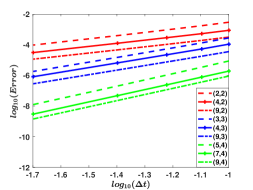
Figure 4: Example 1. The second order methods are in red, third order in blue, and fourth order in green. The eSSPIFRK methods with $(s,p)=(2,2),(3,3),(5,4)$ have a dashed line, those with $(s,p)=(4,2),(4,3),(7,4)$ have a solid line, and those with $s=9$ have a dot-dash line. On the left is splitting (a) while on the right is splitting (b).

While the splitting affects the magnitude of the errors, we see that the order of the errors is not affected. As expected, the error constants are smaller for methods with more stages.

Note that we used a van der Pol problem that is not highly oscillatory. This is because we wish to avoid the order reduction that is known to occur with integrating factor methods. This convergence study purposely avoids this issue in order to test the formal convergence of the generated methods.

6.2 Example 2: Accuracy study

Consider the

$$u_{t}+10u_{x}+\left(\frac{1}{2}u^{2}\right)_{x} =0\hskip 54.2025ptu(0,x)=e^{\sin(2\pi x)}$$ (23)

on the domain $0\leq x\leq 1$. We use a first order upwind finite difference to spatially discretize the linear advection term and the fifth order WENO for the nonlinear term. We use $64$ points in space and the globalorder.m script in the package EXPINT [7, 6] with its built-in exponential time-differencing (ETD) Runge–Kutta methods of orders $p=2,3,4$ (the schemes by Cox and Matthews called ETDRK2, ETDRK3, and ETDRK4 in EXPINT) and our eSSPIFRK methods with $(s,p)=(2,2),(3,3),(5,4)$. The globalorder.m script uses MATLAB’s embedded ODE15s with $AbsTol=10^{-15}$ and $RelTol=5\times 10^{-14}$ to compute the highly accurate reference solution. In Figure 5 (left) we observe that the eSSPIFRK methods are competitive with the ETD methods in terms of accuracy. Despite the fact that we see order reduction in the third and fourth order eSSPIFRK methods, the accuracy of these methods is comparable to that of the corresponding ETD method.

A comparison of the CPU times needed for a given level of accuracy in Figure 5 (right) reveals that the ETD methods are generally somewhat more efficient on this smooth problem. However, we will see below that the ETD methods in fact require inefficiently small time-steps for nonlinear stability in problems with discontinuities that are of interest to us.

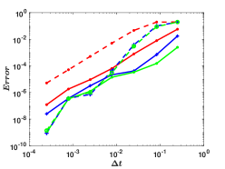
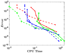
Figure 5: Example 2. The second order methods are in red, third order in blue, and fourth order in green, dashed lines represent the ETD methods while solid lines are the eSSPIFRK methods.

6.3 Example 3: Sharpness of SSP time-step for a linear problem

We consider the linear advection equation with a step function initial condition:

$$u_{t}+au_{x}+u_{x} =0\hskip 54.2025ptu(0,x)=\begin{cases}1,&\text{if }\frac{1}{4}\leq x\leq\frac{3}{4}\\ 0,&\text{else }\end{cases}$$

on the domain $[0,1]$ with periodic boundary conditions. We use a first-order forward difference for each of the spatial derivatives to semi-discretize this problem on a grid of $0\leq x\leq 1$ with 1000 points in space and evolve it ten time-steps forward.

It is known that this spatial discretization when coupled with forward Euler is TVD, under the time-step restriction $\tilde{\Delta t}_{\textup{FE}}=\frac{1}{a}\Delta x$ for the term $Lu\approx au_{x}$, and the restriction $\Delta t_{\textup{FE}}=\Delta x$ for the term $N(u)\approx u_{x}$.

We measure the total variation of the numerical solution at each stage (to ensure internal stage monotonicity), and compare it to the total variation at the previous stage. We are interested in the size of time-step $\Delta t$ at which the total variation begins to rise. We refer to this value as the observed TVD time-step $\Delta t^{TVD}_{obs}$. We compare this value with the expected TVD time-step dictated by the theory. We call the SSP coefficient corresponding to the value of the observed TVD time-step the observed SSP coefficient $\mathcal{C}_{obs}$. Note that the expected TVD time-step $\Delta t_{\textup{FE}}=\Delta x$, so that

$$\mathcal{C}_{obs}=\frac{\Delta t^{TVD}_{obs}}{\Delta t_{\textup{FE}}}=\frac{\Delta t^{TVD}_{obs}}{\Delta x}=\lambda^{TVD}_{obs}.$$

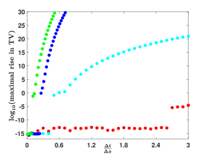
Figure 6: Example 3: Linear advection with a step function initial condition and $a=10$. The eSSPRK(5,3) method is in blue, the eSSPKG(5,3) in green, the IMEXSSP(5,3,$K=0.1$) method in cyan, and the eSSPIFRK(5,3) in red.

6.3.1 Comparison of integrating methods for wavespeed $a=10$

First we consider this problem with wavespeed $a=10$. In Figure 6, we show the observed maximal rise in total variation (on the y-axis) when this equation is evolved forward by a variety of methods using different values of the Courant number $\lambda=\frac{\Delta t}{\Delta x}$ (on the x-axis).

Two methods, eSSPRK(5,3) (blue) from [28] and eSSPKG(5,3) (green) generated in this work, treat the two spatial terms in the same manner. In other words, they evolve the linear advection problem with wavespeed $(1+a)=11$. As expected, the observed time-step before the total variation begins to rise is given by the SSP coefficient scaled by the wavespeed. Our numerical results (represented in Figure 6) show that the eSSPRK(5,3) method has an allowable Courant number $\lambda^{TVD}_{obs}=\frac{\mathcal{C}}{11}=\frac{2.6506}{11}=0.2409$ before the maximal total variation begins to rise. On the other hand, the SSP Kinnmark and Gray method eSSPKG(5,3) has a smaller allowable value of $\lambda^{TVD}_{obs}=\frac{\mathcal{C}}{11}=\frac{1}{11}=0.0909$ before the maximal total variation begins to rise.

Next, we turn our attention to IMEX methods. As shown in [16] both the implicit and explicit terms have to be SSP, and the wavespeed impacts the size of the allowable SSP time-step, even though the fast wave is treated implicitly. We use the SSP implicit-explicit IMEX(5,3,$K=0.1$) method (in cyan) where the slow wave $u_{x}$ is treated explicitly and the fast wave $10u_{x}$ is treated implicitly. We use the IMEX(5,3,$K=0.1$) method found in [16], which is specially optimized in terms of the allowable SSP time-step for the value of $K=\frac{1}{a}=0.1$. This method has a $\mathcal{C}=0.407$ for the value $a=10$. As predicted, the observed time-step before the total variation begin to rise is $\lambda^{TVD}_{obs}=\frac{\mathcal{C}}{10}=0.407$. We see here that using an IMEX SSP method where the fast moving wave is treated implicitly does not give us much benefit when we are concerned with the TVD behavior of the scheme: it allows us only an increase of 69% in time-step, at the major cost of an implicit solve.

Finally, we use the eSSPIFRK(5,3) method (in red) resulting from using our eSSPRK+(5,3) method in formulation (2) where $N(u)=-Du$ and $Lu=-10Du$. This method has a SSP coefficient $\mathcal{C}=2.635$ for any value of $a$ and indeed we observe that the allowable time-step before we see a rise in the total variation is $\Delta t^{TVD}_{obs}=\frac{\mathcal{C}}{\Delta x}$. This means that the largest allowable time-step for the eSSPIFRK(5,3) is more than ten times larger than that for the eSSPRK(5,3), and more than six times larger than for the IMEX method. Additionally, this result is produced without much additional cost, as the few matrix exponentials needed are pre-computed once for the entire simulation. Results of the allowable SSP values for more methods are presented in Table 8 below.

6.3.2 Considering different wavespeeds

The main advantage of the SSP integrating factor Runge–Kutta schemes is that the allowable SSP time-step is not impacted by the wavespeed. In this section, we show how the new eSSPIFRK methods perform equally well for different wavespeeds, and how other methods (including IMEX methods) do not.

Using $a=0$, we verify the expected TVD time-step for most of the methods considered (Table 6). However, we observed that for the methods eSSPIFRK(3,3) and eSSPIFRK(5,4), $\mathcal{C}_{obs}>\mathcal{C}$. For the eSSPIFRK(3,3) method, $\mathcal{C}=\frac{3}{4}$ but the observed value is $\mathcal{C}_{obs}=1$. This is easy to understand because for this linear problem with no exponential component ($a=0$), all methods with the same number of stages as order ($s=p$) are equivalent. Thus, for this special case, our eSSPIFRK(3,3) method can be re-arranged into the eSSPRK(3,3) Shu-Osher method, and we observe the expected TVD time-step for that method. A similar phenomenon occurs for the eSSPIFRK(5,4) method. In this case, we can write the stability polynomial of each stage recursively. If we look at the stability polynomial $P(z)$ of the fourth stage, we observe that its third derivative becomes negative at $z=1.5594$, which is precisely the observed TVD time-step for this method. When we look into the stages to see where the rise in TV occurs, we see that it first happens in the fourth stage of the first time-step.

Method	$\mathcal{C}$	$\lambda^{TVD}_{obs}$
		for $a=0$	$a=1.0$	$a=10$	$a=20$
eSSPIFRK(2,2)	1	1	1	1	1
eSSPIFRK(9,2)	8	8	8	8	8
eSSPIFRK(3,3)	3/4	1	3/2	3/2	3/2
eSSPIFRK(4,3)	20/11	20/11	20/11	20/11	20/11
eSSPIFRK(9,3)	6	6	6	6	6
eSSPIFRK(5,4)	1.346	1.5594	2.158	2.158	2.158
eSSPIFRK(6,4)	2.273	2.273	2.273	2.273	2.273
eSSPIFRK(9,4)	4.306	4.306	4.306	4.306	4.306

Table 6: The observed SSP coefficient compared to the predicted SSP coefficient for Example 3 with various wavespeeds $a$. The value of $a$ does not negatively impact the observed SSP coefficient.

Next, we consider various values of $a>0$. The results in Table 6 confirm that the value of $a$ does not negatively impact the observed SSP coefficient for this linear example. In these cases too, we observe that for most methods the SSP condition is sharp, i.e, $\mathcal{C}_{obs}=\mathcal{C}$ for all values of $a$. The observed TVD time-step for eSSPIFRK(3,3) and eSSPIFRK(5,4) are, once again, larger than expected. For the eSSPIFRK(3,3) method $\mathcal{C}_{obs}=\frac{3}{2}$ is a result of the rise in TV from the first stage, which has a step-size $\frac{2}{3}\Delta t$.

Finally, we compare the eSSPIFRK(4,3) method to the explicit SSP Runge–Kutta method and to IMEX methods. Table 7 shows that the value of $a$ does not negatively impact the observed SSP coefficient for the eSSPIFRK method. When the eSSPRK(4,3) method is applied to the linear advection problem with wavespeed $a+1$, the observed SSP coefficient matches the predicted

$$\lambda^{TVD}_{obs}=\frac{\mathcal{C}_{obs}}{a+1}=\frac{\mathcal{C}}{a+1}=\frac{2}{a+1}$$

as shown in Table 7. We also show the observed SSP coefficient for the SSP IMEX methods IMEXSSP(4,3,K) from [16]. These methods have SSP explicit and implicit parts and were optimized for the SSP step size for each value of $K=\frac{1}{a}$ in [16]. As we expect from SSP theory, the observed value of $\lambda$ before a rise in total variation occurs decays linearly as the wavespeed $a$ rises.

Method	$\lambda^{TVD}_{obs}$
	$a=0$	$a=1.0$	$a=2$	$a=10$	$a=20$	$a=100$
eSSPIFRK(4,3)	1.818	1.818	1.818	1.818	1.818	4.200
SSPIMEX(4,3,K )	2.000	1.476	1.192	0.310	0.162	0.033
eSSPRK(4,3)	2.000	1.000	0.666	0.181	0.0952	0.019

Table 7: The observed SSP coefficients for an eSSPIFRK method, IMEX method, and explicit Runge–Kutta method for Example 3 with various wavespeeds $a$. The value of $a$ does not negatively impact the observed SSP coefficient for the eSSPIFRK method, but it does for the IMEX and the explicit Runge–Kutta methods.

6.3.3 Comparison to linear stability properties

In Figure 6 we notice that for each method, as the Courant number $\lambda=\frac{\Delta t}{\Delta x}$ gets large enough, the maximal rise in total variation jumps up. For some methods, this happens for very small values of $\lambda$, while for others, it happens when $\lambda$ is larger. It is interesting to see how this $\lambda^{TVD}$ allowable for the TVD property compares to the CFL number $\lambda^{L_{2}}$ allowed for linear stability for this problem. Once again, we use $a=10$ and compare the allowable time-step for linear stability and the allowable predicted and observed TVD time-step in Table 8. We evaluate the allowable time-step for linear stability of a given method for this particular problem by calculating the stability polynomial for these operators and determining at which value of $\lambda^{L_{2}}$ the $L_{2}$ norm of the resulting matrix becomes greater than one.

We notice that linear stability does not provide any prediction on the TVD behavior of these methods. The most striking example of this is when looking at the IMEX methods; in terms of linear stability, these can clearly eliminate the constraint coming from the fast wave (e.g., IMEXSSP(3,3,$K=\infty$)), and provide a large region of linear stability. However, this method fails to be SSP for any positive time-step. Even a specially designed and optimized SSP IMEX method did not even double the allowable time-step for TVD.

These results underscore the fact that when solving problems with discontinuities, the relevant time step restriction is dictated by $\lambda^{TVD}$ rather than $\lambda^{L_{2}}$. The most notable result from this table is that all the integrating factor methods have a very large $L_{2}$ linear stability region for this problem. In fact, we tested them up to $\lambda=27$, which is ten times larger than the largest allowable time-step for TVD, and they were still stable at this value. Clearly, the integrating approach has advantages for linear stability as well as for strong stability preservation.

We also note from the results in Table 8 that although the Kinnmark and Gray methods are designed to have larger imaginary axis linear stability regions, for our problem this does not give them an advantage even for linear stability. This is easily understood when we consider that the eigenvalues of our differentiation operator are a circle in the complex plane, and so the linear stability regions of the regular eSSPRK methods are better suited than those of the eSSPKG methods of Kinnmark and Gray (as seen in Figure 3).

Method	$\lambda^{L_{2}}_{obs}$	$\lambda^{TVD}_{pred}$	$\lambda^{TVD}_{obs}$
eSSPRK(3,3)	0.114	1/11	0.090
eSSPKG(3,3)	0.114	1/11	0.090
eSSPRK+(3,3)	0.114	3/44	0.090
eSSPKG+(3,3)	0.114	1/11	0.090
IMEXSSP(3,3,$K=0.1$))	0.448	0.149	0.236
IMEXSSP(3,3,$K=\infty$))	1.198	0.000	0.000
eSSPIFKG(3,3)	*	0.750	1.500
eSSPIFRK(3,3)	*	0.750	1.500
eSSPRK(5,3)	0.260	0.240	0.240
eSSPKG(5,3)	0.138	1/11	0.090
eSSPRK+(5,3)	0.261	0.239	0.239
eSSPKG+(5,3)	0.138	1/11	0.090
IMEXSSP(5,3,$K=0.1$)	0.683	0.407	0.407
eSSPIFKG(5,3)	*	0.875	1.487
eSSPIFRK(5,3)	*	2.635	2.635
eSSPRK(6,4)	0.273	0.208	0.208
eSSPKG(6,4)	0.146	1/11	0.090
eSSPRK+(6,4)	0.270	0.206	0.206
eSSPKG+(6,4)	0.146	0.071	0.090
eSSPIFKG(6,4)	*	0.785	1.805
eSSPIFRK(6,4)	*	2.273	2.273

Table 8: The values of the observed CFL number $\lambda^{L_{2}}=\frac{\Delta t}{\Delta x}$ required for $L_{2}$ linear stability for Example 3: $u_{t}+u_{x}+10u_{x}=0$, compared to the predicted and observed values $\lambda^{TVD}$. An * indicates that these methods were linearly $L_{2}$ stable for the largest values tested, $\lambda\leq 27$.

6.4 Example 4: Sharpness of SSP time-step for a nonlinear problem

Consider the equation:

$$u_{t}+au_{x}+\left(\frac{1}{2}u^{2}\right)_{x} =0\hskip 54.2025ptu(0,x)=\begin{cases}1,&\text{if }0\leq x\leq 1/2\\ 0,&\text{if }x>1/2\end{cases}$$

on the domain $[0,1]$ with periodic boundary conditions. We used a first-order upwind difference to semi-discretize this linear term, and a fifth order WENO finite difference for the nonlinear terms. We solved this problem on a spatial grid with 400 points and evolved it forward 25 time steps using $\Delta t=\lambda\Delta x$. We measured the total variation at each stage, and calculated the maximal rise in total variation over each stage for these 25 time steps.

In Figure 7 (left) we use the value of $a=5$ and graph the $log_{10}$ of the maximal rise in total variation versus the ratio $\lambda=\frac{\Delta t}{\Delta x}$. We observe that our eSSPIFRK(3,3) method (3) maintains a very small maximal rise in total variation until close to $\lambda=0.8$, while the fully explicit third order Shu-Osher method begins to feature a large rise in total variation for a much smaller value of $\lambda=.15\approx\frac{1}{1+a}$. In contrast, the three-stage third order ETD Runge–Kutta [17] and the integrating factor method based on the Shu-Osher method (3) both have a maximal rise in total variation that increases rapidly with $\lambda$.

In Figure 7 (right) we show a similar study using wavespeed $a=10$ and fourth order methods. versus the ratio $\lambda=\frac{\Delta t}{\Delta x}$. We observe that our eSSPIFRK(5,4), eSSPIFRK(6,4), and eSSPIFRK(9,4) methods maintain a very small maximal rise in total variation until close to $\lambda=1.06,1.21,2.41$, respectively. In comparison, the SSP IMEX (5,4) method features an observed $\lambda$ value of $\lambda_{obs}=.25$, the fully explicit SSPRK(10,4) has $\lambda_{obs}=0.58$, and the maximal total variation from the simulation using the ETDRK4 method starts rising rapidly from the smallest value of $\lambda$.

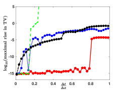
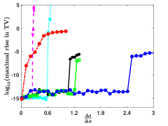
Figure 7: Example 4. Left: $a=5$. The red solid line is the eSSPIFRK(3,3) method, the blue dotted line is the IFRK method based on the eSSPRK(3,3) Shu-Osher method, the black dash-dot line is the ETDRK3 method, and the green dashed line is the third order explicit eSSPRK(3,3) Shu-Osher method. Right: $a=10$. The dashed magenta line with x markers is the SSP IMEX (5,4) method. The dash-dot red line with filled circle markers is the ETDRK4 method. The dotted cyan line with + markers is the SSPRK(10,4) method by Ketcheson The solid lines are the SSPIFRK methods: the black line with star markers for (5,4), green line with square markers for (6,4) and blue line with circle markers for (9,4).

7 Conclusions

This is the first work to consider strong stability preserving integrating factor Runge–Kutta methods. In this work we presented sufficient conditions for preservation of strong stability for integrating factor Runge–Kutta methods. These eSSPIFRK methods are based on eSSPRK methods with non-decreasing abscissas. We used these conditions to develop an optimization problem which we used to find such eSSPRK⁺ methods. We then showed that these eSSPIFRK methods perform in practice as expected, significantly out-performing the implicit-explicit (IMEX) SSP Runge–Kutta methods and the ETD methods of Cox and Matthews on problems that require the SSP property.

Acknowledgment. This publication is based on work supported by AFOSR grant FA9550-15-1-0235. The authors thank David Ketcheson and the anonymous referees for their helpful remarks on this work.

References

- [1]
- [2] A.H. Al Mohy and N.J. Higham, Computing the action of the matrix exponential of a matrix, with an application to exponential integrators, SIAM Journal on Scientific Computing 33(2) (2011), pp. 488–511.
- [3] L. Baiotti, I. Hawke, P.J. Montero, F. Loffler, L. Rezzolla, N. Stergioulas, J.A. Font and E. Seidel. Three-dimensional relativistic simulations of rotating neutron-star collapse to a Kerr black hole. Physical Review D 71 (2005), pp. 24–35.
- [4] J. Balbás and E. Tadmor. A central differencing simulation of the Orszag-Tang vortex system, IEEE Transactions on Plasma Science 33 (2005), pp.470–471.
- [5] E. Bassano, Numerical simulation of thermo-solutal-capillary migration of a dissolving drop in a cavity, International Journal for Numerical Methods in Fluids 41 (2003), pp. 765–788.
- [6] H. Berland, B. Skaflestad, and W. M. Wright, Expint – a MATLAB package for exponential integrators, 2005.
- [7] H. Berland, B. Skaflestad, and W. M. Wright, Expint – a MATLAB package for exponential integrators, ACM Transactions in Mathematical Software, 33 (2007).
- [8] J.C. Butcher, The numerical analysis of ordinary differential equations: Runge-Kutta and general linear methods, Wiley-Interscience New York, NY, USA 1987
- [9] R. Caiden, R.P. Fedkiw and C. Anderson, A numerical method for two-phase flow consisting of separate compressible and incompressible regions, Journal of Computational Physics 166 (2001), pp. 1–27.
- [10] J. Carrillo, I.M. Gamba, A. Majorana and C.-W. Shu, A WENO-solver for the transients of Boltzmann-Poisson system for semiconductor devices: performance and comparisons with Monte Carlo methods, Journal of Computational Physics 184 (2003), pp. 498–525.
- [11] L.-T. Cheng, H. Liu and S. Osher, Computational high-frequency wave propagation using the level set method, with applications to the semi-classical limit of Schrodinger equations, Communications in Mathematical Sciences 1 (2003), pp. 593–621.
- [12] V. Cheruvu, R.D. Nair and H.M. Tufo, A spectral finite volume transport scheme on the cubed-sphere, Applied Numerical Mathematics 57 (2007), pp. 1021–1032.
- [13] B. Cockburn and C.-W. Shu, TVB Runge-Kutta local projection discontinuous Galerkin finite element method for conservation laws II: general framework, Mathematics of Computation 52 (1989), pp. 411–435.
- [14] B. Cockburn, F. Li and C.-W. Shu, Locally divergence-free discontinuous Galerkin methods for the Maxwell equations, Journal of Computational Physics 194 (2004), pp. 588–610.
- [15] B. Cockburn, J. Qian, F. Reitich and J. Wang, An accurate spectral/discontinuous finite-element formulation of a phase-space-based level set approach to geometrical optics, Journal of Computational Physics 208 (2005), pp. 175–195.
- [16] S. Conde, S. Gottlieb, Z. Grant, J.N. Shadid, Implicit and Implicit-Explicit Strong Stability Preserving Runge Kutta Methods with High Linear Order, Journal of Scientific Computing 73(2) (2017), pp. 667–690.
- [17] S. Cox and P. Matthews, Exponential time differencing for stiff systems, Journal of Computational Physics, 176 (2002), pp. 430–455.
- [18] L. Del Zanna and N. Bucciantini, An efficient shock-capturing central-type scheme for multidimensional relativistic flows: I. hydrodynamics, Astronomy and Astrophysics 390 (2002), pp. 1177–1186.
- [19] D. Enright, R. Fedkiw, J. Ferziger and I. Mitchell. A hybrid particle level set method for improved interface capturing. Journal of Computational Physics, 183:83–116, 2002.
- [20] L.-L. Feng, C.-W. Shu and M. Zhang, A hybrid cosmological hydrodynamic/n-body code based on a weighted essentially nonoscillatory scheme, The Astrophysical Journal 612 (2004), pp. 1–13.
- [21] L. Ferracina and M.N. Spijker, Stepsize restrictions for the total-variation-diminishing property in general Runge-Kutta methods, SIAM Journal of Numerical Analysis 42 (2004), pp. 1073-1093.
- [22] L. Ferracina and M.N. Spijker, An extension and analysis of the Shu-Osher representation of Runge-Kutta methods, Mathematics of Computation 249(2005), pp. 201–219.
- [23] L. Ferracina and M.N. Spijker, Strong stability of singly-diagonally-implicit Runge-Kutta methods, Applied Numerical Mathematics 2008
- [24] S. Gaudreault, G. Rainwater, M. Tokman, KIOPS: A fast adaptive Krylov subspace solver for exponential integrators, arXiv:1804.05126 [math.NA] (2018).
- [25] D. Gottlieb and J.S. Hesthaven, Spectral methods for hyperbolic problems, Journal of Computational and Applied Mathematics, 128 (2001), pp. 83-131.
- [26] D. Gottlieb and E. Tadmor The CFL condition for spectral approximations to hyperbolic initial-boundary value problems, Mathematics of Computation 56 (1991), pp. 565–588.
- [27] S. Gottlieb, Z. Grant, and L. Isherwood, Optimized strong stability preserving integrating factor Runge–Kutta methods. https://github.com/SSPmethods/SSPIFRK-methods.
- [28] S. Gottlieb, D. I. Ketcheson, and C.-W. Shu, Strong Stability Preserving Runge–Kutta and Multistep Time Discretizations, World Scientific Press, 2011.
- [29] S. Gottlieb and C.-W. Shu, Total variation diminishing Runge–Kutta methods, Mathematics of Computation, 67 (1998), pp. 73–85.
- [30] S. Gottlieb, C.-W. Shu, and E. Tadmor, Strong Stability Preserving High-Order Time Discretization Methods, SIAM Review, 43 (2001), pp. 89–112.
- [31] A. Harten, High resolution schemes for hyperbolic conservation laws, Journal of Computational Physics, 49 (1983), pp. 357–393.
- [32] J.S. Hesthaven, Numerical methods for conservation laws: From analysis to algorithms, SIAM Publishing, Philadelphia (2017).
- [33] J.S. Hesthaven, S. Gottlieb, and D. Gottlieb, Spectral Methods for Time Dependent Problems, Cambridge Monographs on Applied and Computational Mathematics (No. 21) Cambridge University Press (2006).
- [34] I. Higueras, On strong stability preserving time discretization methods, Journal of Scientific Computing 21 (2004), pp. 193–223.
- [35] I. Higueras, Representations of Runge-Kutta methods and strong stability preserving methods, SIAM Journal on Numerical Analysis 43 (2005), pp. 924–948.
- [36] X. Y. Hu, N. A. Adams, and C.-W. Shu, Positivity-preserving method for high-order conservative schemes solving compressible Euler equations, Journal of Computational Physics 242 (2013), pp. 169–180.
- [37] W. Hundsdorfer, S.J. Ruuth and R.J. Spiteri, Monotonicity-preserving linear multistep methods, SIAM Journal on Numerical Analysis 41 (2003), pp. 605–623.
- [38] S. Jin, H. Liu, S. Osher and Y.-H.R. Tsai, Computing multivalued physical observables for the semiclassical limit of the Schrodinger equation, Journal of Computational Physics 205 (2005), pp. 222–241.
- [39] C.A. Kennedy, M.H. Carpenter, and R.M. Lewis, Low-storage explicit Runge–Kutta schemes for the compressible Navier-Stokes equations, Applied Numerical Mathematics 35 (2000), pp. 177-219.
- [40] D. I. Ketcheson, Highly efficient strong stability preserving Runge–Kutta methods with low-storage implementations, SIAM Journal on Scientific Computing, 30 (2008), pp. 2113–2136.
- [41] D.I. Ketcheson, C.B. Macdonald and S. Gottlieb, Optimal implicit strong stability preserving Runge-Kutta methods, Applied Numerical Mathematics 52 (2009), pp. 373–392.
- [42] D. I. Ketcheson, Computation of optimal monotonicity preserving general linear methods, Mathematics of Computation 78 (2009), pp. 1497–1513.
- [43] D. I. Ketcheson, Step sizes for strong stability preservation with downwind-biased operators, SIAM Journal on Numerical Analysis 49 (4) (2011), pp. 1649–1660.
- [44] Kinnmark and Gray, One step integration methods with maximum stability regions, Mathematics and Computers in Simulation 26 (2) (1984), pp. 87–92.
- [45] J. F. B. M. Kraaijevanger, Contractivity of Runge–Kutta methods, BIT, 31 (1991), pp. 482–528.
- [46] E.J. Kubatko, B. A. Yeager, and D. I. Ketcheson, Optimal strong-stability-preserving Runge Kutta time discretizations for discontinuous Galerkin methods, Journal of Scientific Computing 60(2) (2014), pp. 313–344.
- [47] A. Kurganov and E. Tadmor, New high-resolution schemes for nonlinear conservation laws and convection-diffusion equations, Journal of Computational Physics 160 (2000), pp. 241–282.
- [48] S. Labrunie, J. Carrillo and P. Bertrand, Numerical study on hydrodynamic and quasi-neutral approximations for collisionless two-species plasmas, Journal of Computational Physics 200 (2004), pp. 267–298.
- [49] J. D. Lawson, Generalized Runge-Kutta Processes for Stable Systems with Large Lipschitz Constants, SIAM Journal on Numerical Analysis, 4(3) (1967), pp. 372–380.
- [50] P.D. Lax, Gibbs Phenomena, Journal of Scientific Computing, 28 (2006), pp. 445–449.
- [51] H.W.J. Lenferink, Contractivity-preserving implicit linear multistep methods, Mathematics of Computation 56 (1991), pp. 177–199.
- [52] R. J. LeVeque, Numerical Methods for Conservation Laws, ETH Lectures in Mathematics Series, Birkhauser-Verlag, (1990).
- [53] D. Levy and E. Tadmor, From Semi-Discrete to Fully-Discrete: The Stability of Runge-Kutta Schemes by the Energy Method, SIAM Review, 40(1) (1998), pp. 40–73.
- [54] X.-D. Liu, S. Osher and T. Chan, Weighted essentially non-oscillatory schemes, Journal of Computational Physics 115(1) (1994), pp. 200–212.
- [55] H. Ma, Chebyshev–Legendre super spectral viscosity method for nonlinear conservation laws, SIAM Journal on Numerical Analysis 35(3) (1998), pp. 893–908.
- [56] Y. Maday and E. Tadmor, Analysis of the spectral vanishing viscosity method for periodic conservation laws, SIAM Journal on Numerical Analysis 26 (1989), pp. 854-870.
- [57] A. Majda and S. Osher, A systematic approach for correcting nonlinear instabilities. the Lax-Wendroff scheme for scalar conservation laws, Numerische Mathematik 30 (1978), pp. 429–452.
- [58] A. Mignone, The dynamics of radiative shock waves: linear and nonlinear evolution, The Astrophysical Journal 626 (2005), pp. 373–388.
- [59] G. Golub and C. Van Loan, Nineteen Dubious Ways to Compute the Exponential of a Matrix, Twenty-Five Years Later. SIAM Review 45 (2003), pp. 801–836.
- [60] J. Niesen and W.M. Wright, Algorithm 919: A Krylov subspace algorithm for evaluating the -functions appearing in exponential integrators, ACM Transactions on Mathematical Software 38(3) (2012), pp. 22.
- [61] S. Osher and S. Chakravarthy, High resolution schemes and the entropy condition, SIAM Journal on Numerical Analysis 21 (1984), pp. 955–984.
- [62] C. Pantano, R. Deiterding, D.J. Hill and D.I. Pullin, A low numerical dissipation patch-based adaptive mesh refinement method for large-eddy simulation of compressible flows, Journal of Computational Physics 221 (2007), pp. 63–87.
- [63] S. Patel and D. Drikakis, Effects of preconditioning on the accuracy and efficiency of incompressible flows, International Journal for Numerical Methods in Fluids 47 (2005), pp. 963–970.
- [64] D. Peng, B. Merriman, S. Osher, H. Zhao and M. Kang, A PDE-based fast local level set method, Journal of Computational Physics 155 (1999), pp. 410–438.
- [65] S. C.Reddy and L. N.Trefethen, Lax stability of fully discrete spectral methods via stability regions and pseudo-eigenvalues, Computer Methods in Applied Mechanics and Engineering 80(1 3) (1990), pp. 147–164.
- [66] S. J. Ruuth and R. J. Spiteri, Two barriers on strong-stability-preserving time discretization methods, Journal of Scientific Computation, 17 (2002), pp. 211–220.
- [67] C.-W. Shu, TVB uniformly high-order schemes for conservation laws, Mathematics of Computation 49 (1987), pp. 105–121.
- [68] C.-W. Shu, Total-variation diminishing time discretizations, SIAM Journal on Scientific Statistical Computing 9 (1988), pp. 1073–1084.
- [69] C.-W. Shu and S. Osher, Efficient implementation of essentially non-oscillatory shock-capturing schemes, Journal of Computational Physics 77 (1988), pp. 439–471.
- [70] R.B. Sidje, EXPOKIT: A software package for computing matrix exponentials, ACM Transactions on Mathematical Software 24(1) (1998), pp. 130–156.
- [71] M.N. Spijker, Contractivity in the numerical solution of initial value problems, Numerische Mathematik 42 (1983), pp. 271–290.
- [72] M. Spijker, Stepsize conditions for general monotonicity in numerical initial value problems, SIAM Journal on Numerical Analysis, 45 (2008), pp. 1226–1245.
- [73] R. J. Spiteri and S. J. Ruuth, A new class of optimal high-order strong-stability-preserving time discretization methods, SIAM Journal on Numerical Analysis, 40 (2002), pp. 469–491.
- [74] G. Strang, Accurate partial difference methods II: nonlinear problems, Numerische Mathematik 6 (1964), pp. 37–46.
- [75] J.C. Strikwerda, Finite Difference Schemes and Partial Differential Equations, Cole Mathematics Series. Wadsworth and Brooks, California, 1989.
- [76] Y. Sun, Z.J. Wang and Y. Liu, Spectral (finite) volume method for conservation laws on unstructured grids VI: Extension to viscous flow., Journal of Computational Physics, 215 (2006), pp. 41–58.
- [77] P.K. Sweby, High resolution schemes using flux limiters for hyperbolic conservation laws, SIAM Journal on Numerical Analysis 21 (1984), pp. 995–1011.
- [78] E. Tadmor, Advanced Numerical Approximation of Nonlinear Hyperbolic Equations,” Lectures Notes from CIME Course Cetraro, Italy, 1997, pp 1–150 in Approximate solutions of nonlinear conservation laws, Number 1697 in Lecture Notes in Mathematics. Springer-Verlag, 1998,
- [79] E. Tadmor, Shock capturing by the spectral viscosity method, Computer Methods in Applied Mechanics and Engineering 80 (1990), pp. 197-208.
- [80] M. Tanguay and T. Colonius, Progress in modeling and simulation of shock wave lithotripsy, In Fifth International Symposium on cavitation (CAV2003), OS-2-1-010, 2003.
- [81] P.J. van der Houwen, Explicit Runge–Kutta formulas with increased stability boundaries, Numerische Mathematik 20 (1972), pp. 149-164.
- [82] Z.J. Wang and Y. Liu, The spectral difference method for the 2D Euler equations on unstructured grids, In 17th AIAA Computational Fluid Dynamics Conference, AIAA, 2005.
- [83] Z.J. Wang, Y. Liu, G. May and A. Jameson, Spectral difference method for unstructured grids II: Extension to the Euler equations, Journal of Scientific Computing 32(1) (2007), pp. 45–71.
- [84] J. H. Williamson, Low storage Runge–Kutta schemes, Journal of Computational Physics, 35 (1980), pp. 48-56.
- [85] W. Zhang and A.I. MacFayden, RAM: A relativistic adaptive mesh refinement hydrodynamics code, The Astrophysical Journal Supplement Series 164 (2006), pp. 255–279.
- [86] X. Zhang and C.-W. Shu, On maximum-principle-satisfying high order schemes for scalar conservation laws, Journal of Computational Physics 229 (2010), pp. 3091–3120.
- [87] X. Zhang and C.-W. Shu, On positivity-preserving high order discontinuous Galerkin schemes for compressible Euler equations on rectangular meshes. Journal of Computational Physics 229 (2010), pp. 8918–8934.
- [88] X. Zhang and C.-W. Shu, Maximum-principle-satisfying and positivity-preserving high-order schemes for conservation laws: survey and new developments, Proceedings of the Royal Society A 467 (2011), pp. 2752–2776.
- [89] X. Zhang and C.-W. Shu, Positivity-preserving high order discontinuous Galerkin schemes for compressible Euler equations with source terms, Journal of Computational Physics 230 (2011), pp. 1238–1248.
- [90] X. Zhang and C.-W. Shu, Positivity-preserving high order finite difference WENO schemes for compressible Euler equations, Journal of Computational Physics 231 (2012), pp. 2245–2258.