Strong and radiative decays of excited vector mesons and predictions for a new $\phi(1930)$ resonance

Abstract

We study the phenomenology of two nonets of excited vector mesons, $\{\rho(1450)$, $K^{\ast}(1410)$, $\omega(1420)$, $\phi(1680)\}$ and $\{\rho(1700),$ $K^{\ast}(1680),\omega(1650),$ $\phi(???)\},$ which (roughly) correspond to radially excited $2^{3}S_{1}$ and to orbitally excited $1^{3}D_{1}$ vector mesons. We evaluate the strong and radiative decays of these mesons into pseudoscalar and ground-state vector mesons by using an effective relativistic QFT model based on flavour symmetry. We compare decay widths and branching ratios with various experimental results listed in the PDG. An overall agreement of theory with experiment reinforces the standard quark-antiquark assignment of the resonances mentioned above. Predictions for not yet measured quantities are also made. In particular, we shall also make predictions for the not-yet discovered $s\bar{s}$ state of the $1^{3}D_{1}$ nonet, denoted as $\phi(???)$. Its mass can be estimated to be about $1930$ MeV, hence we shall call this putative state $\phi(1930).$ Its main decays are into $KK^{\ast}(892)$ (about $200$ MeV) and $KK$ (about $100$ MeV). Since this state couples also to $\gamma\eta,$ it can be searched in the near future in the photoproduction-based experiments GlueX and CLAS12 at Jefferson Lab.

1 Introduction

Strong interactions are described by Quantum Chromodynamics (QCD). While the degrees of freedom of the QCD Lagrangian are elementary ‘colored’ quarks and gluons, the physical spectrum listed in the PDG [1] consists of ‘white’ hadrons. Hadrons are, in general, bound states of quarks and gluons and are further classified into mesons (bosonic hadrons) and baryons (fermionic hadrons).

The vast majority of mesons consists of ‘conventional’ quark-antiquark states, see the results of the quark model in Ref. [2], but nowadays experimental evidence for non-conventional mesons is mounting, e.g. Refs. [3, 4]. Some known resonances in the low-energy sector might be predominately four-quark state, e.g. Ref. [5], or gluonic, e.g. Ref. [6]; in the energy region of charmonium and bottomonium masses many resonances, the so-called $X,$ $Y$ and $Z$ states, have been found [7]. Similarly, conventional baryons are three-quark states [8], but pentaquark states have been also recently discovered [9].

In this work we concentrate on the light mesonic sector by studying the phenomenology (in particular, strong and radiative decays) of two types of excited quark-antiquark vector mesons. The firm understanding of conventional $\bar{q}q$ states is necessary to look for further non-conventional states with the same quantum numbers. Moreover, the general status of excited states is rather poorly understood and improvement is needed, see the quark model review in the PDG [10]. Excited vector mesons (for some previous theoretical studies on them, see Refs. [11, 12, 13, 14, 15]) are especially interesting in this context for various reasons:

(i) The ground-state vector mesons {$\rho(770),$ $K^{\ast}(892),$ $\phi(1020),$ $\omega(782)$} are very well known and represent an excellent example of an ideal $\bar{q}q$ nonet. The non-relativistic quantum numbers are $(n,L,S)=(1,0,1)$ ($n$ being the principal quantum number, $L$ the spacial angular momentum, and $S$ the spin), hence, in the non-relativistic spectroscopic notation one has $n$ ${}^{2S+1}L_{J}=1$ ${}^{3}S_{1}$ and in the relativistic notation $J^{PC}=1^{--}.$ Considering that the nonet of pseudoscalar meson is special due to the importance of spontaneous symmetry breaking and the axial anomaly, one may say that ground-state vector mesons are the lightest ideal $\bar{q}q$ objects.

(ii) Two types of excited vector mesons have been experimentally measured. Although data need improvement, there is enough information on masses and decays to undertake a systematic analysis. One nonet corresponds (predominantly) to the radial excitation, with the quantum numbers $(n,L,S)=(2,0,1)$ (spectroscopic notation $2^{3}S_{1},$ relativistic notation $J^{PC}=1^{--});$ the associated states are {$\rho(1450)$, $K^{\ast}(1410)$, $\omega(1420)$, $\phi(1680)$}. [Note, there are only two nonets of states with $n=2$ listed in the PDG. Besides vector mesons, a tentative assignment is done also for excited pseudoscalar mesons with $(n,L,S)=(2,0,0),$ for details and references see the recent work in Ref. [16].] The second nonet corresponds (predominantly) to the orbital excitation, i.e. it has quantum numbers $(n,L,S)=(1,2,1)$ (spectroscopic notation $1^{3}D_{1},$ relativistic notation still $J^{PC}=1^{--}$). The associated states are {$\rho(1700)$, $K^{\ast}(1680)$, $\omega(1650)$, $\phi(???)$}. It should be stressed from the very beginning that the physical resonances listed above do not correspond exactly to the mentioned non-relativistic quark-antiquark configurations, but can arise from mixing of them (moreover, a dressing of meson-meson pairs also takes place). Hence we should regard the previous assignment as indicating the predominant contribution.

(iii) The state $\phi(???)$ belonging to the nonet of orbitally excited $1^{3}D_{1}$ states has not yet been observed. It is the last missing state of that nonet, hence the empty space in Table II of Ref. [10]. Its mass can be estimated by the mass differences between the two nonets described above, obtaining $m_{\phi(???)}-m_{\phi(1680)}\simeq$ $m_{\rho(1700)}-m_{\rho(1450)}\simeq 250$ MeV, thus we expect that $\phi(???)$ has a mass of about $1930$ MeV and we therefore postulate the existence of a new resonance, denoted $\phi(1930)$ (note, the value $1930$ MeV is not far from the old quark model prediction of $1880$ MeV [2]).

In this work, we study the decays of the excited vector mesons {$\rho(1450)$, $K^{\ast}(1410)$, $\omega(1420)$, $\phi(1680)$} and {$\rho(1700)$, $K^{\ast}(1680)$, $\omega(1650)$, $\phi(???)\equiv\phi(1930)$} by using a quantum field theoretical (QFT) approach whose d.o.f. are mesons. The fields entering in our model correspond to these resonances and hence roughly, but not exactly, to the quark-antiquark configurations $2^{3}S_{1}$ and $1^{3}D_{1}$ predicted by the quark model (as discussed above mixing is possible). Indeed, a direct link of our vector fields to an underlying microscopic wave function of the quarks is not possible and also not necessary (details later on). The Lagrangian of the model is constructed under the requirement of flavour symmetry (i.e., the invariance under the rotation of the quarks $u,$ $d$, and $s,$ a well proven approximate symmetry of QCD), as well as invariance under parity $P$ and charge conjugation $C$. Indeed, flavour symmetry is present in various approaches of low-energy QCD, such as chiral perturbation theory [17, 18], linear sigma models [19, 20, 21, 22, 23], and also Bethe-Salpeter approaches [24, 25]. Namely, even after spontaneous symmetry breaking (SSB), flavour symmetry is still manifest. The use of flavour symmetric mesonic QFT models, on which our approach is based, has proven to be successful in the past in studies on decays of mesonic multiplets, such as the well-known tensor mesons [26], the pseudovector mesons [27], the pseudotensor mesons [28], and also the more difficult scalar mesons (in which the scalar glueball leaks in) [29, 30]. Here, we shall follow the very same methodology of those works.

To be more specific, we write a Lagrangian that contains the two nonets of excited vector mesons previously mentioned as well as their main decay products: the ground-state vector mesons and pseudoscalar mesons. Moreover, in a second step, we shall also include the photon for radiative decays. When dominant terms in the large-$N_{c}$ expansion are kept, the number of parameter of our Lagrangian is rather small: 4 parameters (2 for each nonet) which allow to calculate a large number of decay rates (about 64 decay rates, 32 per each nonet). As a result, we can check the status of the quark-antiquark assignment for these states and make predictions for decay rates which are poorly known or have not yet been measured. In the PDG there are also many branching ratios which can be compared to our results. We shall find that the overall interpretation as $\bar{q}q$ states is satisfactory, but some points deserve further clarification and more data is needed (fortunately, the experiments GlueX and CLAS12 start operation soon). Then, as a last important step, we will make predictions for the yet undiscovered $\bar{s}s$ state $\phi(???)\equiv\phi(1930)$.

The paper is organized as follows: in Sec. 2 we present the fields of the model, the Lagrangian, the theoretical expressions for the decay widths, as well as the determination of the parameters. Then, in Sec. 3 we present the results (separately for each excited nonet) of the decay widths and compare them to the experimental results. In particular, we shall also discuss various decay ratios. In Sec. 5 we summarize our results and present our outlook, in particular in connection with the putative and yet undiscovered state $\phi(1930)$. Various details are relegated to the appendices.

2 The Model

We use an effective relativistic Quantum Field Theoretical model based on flavour symmetry. The d.o.f. are mesonic fields, which correspond to quark-antiquark states. In this section, we first present the fields of the model and their assignment, then we show the Lagrangian and finally the expressions of the strong and radiative decay widths.

2.1 The fields of the model

As a first step, we introduce four nonets of mesons, which are given in terms of matrices. Intuitively, each matrix corresponds to the following quark-antiquark content:

$$\frac{1}{\sqrt{2}}\left(\begin{array}[c]{lcr}\bar{u}u&\bar{d}u&\bar{s}u\\ \bar{u}d&\bar{d}d&\bar{s}d\\ \bar{u}s&\bar{d}s&\bar{s}s\end{array}\right)\text{ .}$$ (1)

Although strictly speaking only the relativistic notation $J^{PC}$ is relevant in a relativistic QFT treatment, we shall also keep track of the non-relativistic notation for these multiplets, which should be heuristically understood as the dominant contribution in the (in our approach invisible) microscopic wave function of the quark and the antiquark pairs. In this way, a link with the quark model results -although approximate- is possible and allows for a better intuitive understanding of these states. The explicit form of the matrices for the nonet of pseudoscalar mesons, the nonet of ground-state vector mesons, and two nonets of excited vector mesons read:

$$P=\frac{1}{\sqrt{2}}\left(\begin{array}[c]{lcr}\frac{\eta_{N}+\pi^{0}}{\sqrt{2}}&\pi^{+}&K^{+}\\ \pi^{-}&\frac{\eta_{N}-\pi^{0}}{\sqrt{2}}&K^{0}\\ K^{-}&\bar{K}^{0}&\eta_{S}\end{array}\right)\text{ ; }V^{\mu}=\frac{1}{\sqrt{2}}\left(\begin{array}[c]{lcr}\frac{\omega^{\mu}+\rho^{\mu 0}}{\sqrt{2}}&\rho^{\mu+}&K_{i}^{\mu\star+}\\ \rho^{\mu-}&\frac{\omega^{\mu}-\rho^{\mu 0}}{\sqrt{2}}&K^{\mu\star 0}\\ K^{\mu\star-}&\bar{K}^{\mu\star 0}&\phi^{\mu}\end{array}\right)\text{ ; }$$ (2)

$$V_{E}^{\mu}=\frac{1}{\sqrt{2}}\left(\begin{array}[c]{lcr}\frac{\omega_{E}^{\mu}+\rho_{E}^{\mu 0}}{\sqrt{2}}&\rho_{E}^{\mu+}&K_{E}^{\mu\star+}\\ \rho_{E}^{\mu-}&\frac{\omega_{E}^{\mu}-\rho_{E}^{\mu 0}}{\sqrt{2}}&K_{E}^{\mu\star 0}\\ K_{E}^{\mu\star-}&\bar{K}_{E}^{\mu\star 0}&\phi_{E}^{\mu}\end{array}\right)\text{ ; }V_{D}^{\mu}=\frac{1}{\sqrt{2}}\left(\begin{array}[c]{lcr}\frac{\omega_{D}^{\mu}+\rho_{D}^{\mu 0}}{\sqrt{2}}&\rho_{D}^{\mu+}&K_{D}^{\mu\star+}\\ \rho_{D}^{\mu-}&\frac{\omega_{D}^{\mu}-\rho_{D}^{\mu 0}}{\sqrt{2}}&K_{D}^{\mu\star 0}\\ K_{D}^{\mu\star-}&\bar{K}_{D}^{\mu\star 0}&\phi_{D}^{\mu}\end{array}\right)\text{ .}$$ (3)

(For the explicit quark-antiquark microscopic current leading to these fields, see Ref. [28]). The matrix $P$ describes the nonet of pseudoscalar mesons corresponding to the states $\{\pi,K,\eta\equiv\eta(547),\eta^{\prime}\equiv\eta^{\prime}(958)\}.$ Namely, the two fields denoted as $\eta_{N}$ and $\eta_{S}$ in Eq. (2) mix and generate the physical fields $\eta$ and $\eta^{\prime}$:

$$\eta_{N}=\eta\cos\theta_{P}-\eta^{\prime}\sin\theta_{P}\text{ and }\eta_{S}=\eta\sin\theta_{P}-\eta^{\prime}\cos\theta_{P}\text{ .}$$ (4)

The mixing angle $\theta_{P}$ is set to $-42^{\circ}$ [31]. Using other values in the range ($-40^{\circ},$ $-45^{\circ}$), e.g. Refs. [22, 32, 33], would affect only marginally our results. In the non-relativistic notation, this nonet corresponds (predominantly) to $(n,L,S)=(1,0,0),$ hence to $n$ ${}^{2S+1}L_{J}=1$ ${}^{1}S_{0}$. The relativistic notation is $J^{PC}=0^{-+}.$

The nonet of ground-state vector mesons, denoted as $V^{\mu}$, is associated to the resonances $\{\rho(770),$ $K^{\ast}(892),$ $\phi(1020),$ $\omega(782)\}$. Actually, also the bare fields $\omega=\sqrt{1/2}(\bar{u}u+\bar{d}d)$ and $\phi=\bar{s}s$ entering in Eq. (2) mix, but the mixing is sufficiently small to be neglected (about $-3^{\circ},$ [10]); then, $\omega(782)$ is regarded as purely nonstrange and $\phi(1020)$ as purely strange. The nonrelativistic quantum numbers are $(n,L,S)=(1,0,1),$ hence $n$ ${}^{2S+1}L_{J}=1$ ${}^{3}S_{1}$. Relativistically: $J^{PC}=1^{--}.$

Finally, we turn to the excited vector mesons. The matrix $V_{E}^{\mu}$ describes the first nonet of excited vector mesons that we assign to the states {$\rho(1450)$, $K^{\ast}(1410),$ $\omega(1420),$ $\phi(1680)$}. As for vector mesons, we neglect the isoscalar mixing, hence $\omega(1420)$ is purely nonstrange ($\sqrt{1/2}(\bar{u}u+\bar{d}d)$ ) and $\phi(1680)$ purely strange, $\bar{s}s$. This nonet corresponds to (predominantly but not identically) radially excited vector mesons with the non-relativistic quantum numbers $(n,L,S)=(2,0,1),$ hence $n$ ${}^{2S+1}L_{J}=2$ ${}^{3}S_{1}$. Relativistically: $J^{PC}=1^{--}$ (just as the ground-state vector mesons). Note, the state $K^{\ast}(1410)$ has been clearly seen in the recent lattice studies of Ref. [34] while $\omega(1420)$ and $\phi(1680)$ have been observed in the lattice studies of Ref. [35, 36].

The matrix $V_{D}^{\mu}$ describes the second nonet of excited vectors: {$\rho(1700)$, $K^{\ast}(1680)$, $\omega(1650)$, $\phi(???)$}. Also here, the isoscalar mixing is neglected. Non relativistically, this nonet corresponds (always predominantly) to orbitally excited vector mesons with $(n,L,S)=(1,2,1),$ hence $n$ ${}^{2S+1}L_{J}=1$ ${}^{3}D_{1}$. Relativistically: $J^{PC}=1^{--}.$ The $\bar{s}s$ state in the $1^{3}D_{1}$ nonet, denoted as $\phi(???)$, has not yet been experimentally seen. By using our model, we make predictions for this resonance. In order to include this state into our calculation, we have to estimate its mass. In Table 1 we present the masses of the known members of the two nonets. It is visible that the mass difference between radially and orbitally excited vector mesons are approximately the same for all states. The reason for that is the same type of strong dynamics describing these mesons and their masses.

$V_{E}$ $\rho(1450)$ $K^{\ast}(1410)$ $\omega(1420)$ $\phi(1680)$ $V_{D}$ $\rho(1700)$ $K^{\ast}(1680)$ $\omega(1650)$ $\phi(???)$ Difference $250$ MeV $270$ MeV $230$ MeV ?

Table 1: Mass differences between the members of the two nonets of excited vector mesons.

Hence, we can estimate the mass of $\phi(???)$ as:

$$m_{\phi(???)}\simeq(m_{\phi(1680)}+250\pm 20)\text{ MeV}=1930\pm 20\text{ MeV}.$$ (5)

From now on we shall call this hypothetical state

$$\phi(???)\equiv\phi(1930)\text{ .}$$

All the fields have precise transformations under parity $P,$ charge conjugation $C,$ and flavour symmetry $U(3)_{V},$ which are summarized in Table 2.

Parity ($P$) Charge conjugation ($C$) Flavor ($U\left(3\right)_{V}$) $P$ $-P(t,-\vec{x})$ $P^{t}$ $UPU^{\dagger}$ $V^{\mu}$ $V_{\mu}(t,-\vec{x})$ $-\left(V^{\mu}\right)^{t}$ $UV^{\mu}U^{\dagger}$ $V_{E}^{\mu}$ $V_{E,\mu}(t,-\vec{x})$ $-\left(V_{E}^{\mu}\right)^{t}$ $UV_{E}^{\mu}U^{\dagger}$ $V_{D}^{\mu}$ $V_{D,\mu}(t,-\vec{x})$ $-\left(V_{D}^{\mu}\right)^{t}$ $UV_{D}^{\mu}U^{\dagger}$

Table 2: Transformation properties of the nonets under charge, parity, and flavour transformations. Notice that the parity transformation for vector states is obtained by lowering the Lorentz index.

2.2 The Lagrangian

The Lagrangian of the model is obtained by properly coupling the matrices listed above and by requiring invariance under $P,$ $C,$ and $U(3)_{V}.$ It explicitly reads:

$$\mathcal{L}=\mathcal{L}_{EPP}+\mathcal{L}_{DPP}+\mathcal{L}_{EVP}+\mathcal{L}_{DVP}$$ (6)

where

$$\mathcal{L}_{EPP} =ig_{EPP}Tr\left([\partial^{\mu}P,V_{E,\mu}]P\right)\text{ ,\quad}\mathcal{L}_{DPP}=ig_{DPP}Tr\left([\partial^{\mu}P,V_{D,\mu}]P\right)\text{ ,}$$ (7)

$$\mathcal{L}_{EVP} =g_{EVP}Tr\left(\tilde{V}_{E}^{\mu\nu}\{V_{\mu\nu},P\}\right)\text{ ,}\quad\mathcal{L}_{DVP}=g_{DVP}Tr\left(\tilde{V}_{D}^{\mu\nu}\{V_{\mu\nu},P\}\right)\text{ .}$$ (8)

The terms contain various processes: $\mathcal{L}_{EPP}$ describes the decay $V_{E}\rightarrow PP,$ $\mathcal{L}_{DPP}$ the decay $V_{D}\rightarrow PP,$ $\mathcal{L}_{EVP}$ the decay $V_{E}\rightarrow VP$, and finally $\mathcal{L}_{DVP}$ the decay $V_{D}\rightarrow VP.$ The notation $[A,B]=AB-BA$ stands for the usual commutator and $\{A,B\}=AB+BA$ for the anticommutator. Moreover, the dual fields have been defined in the standard way:

$$\tilde{V}_{E}^{\mu\nu}=\frac{1}{2}\epsilon^{\mu\nu\alpha\beta}(\partial_{\alpha}V_{E,\beta}-\partial_{\beta}V_{E,\alpha})\text{ ,}$$ (9)

$$\tilde{V}_{D}^{\mu\nu}=\frac{1}{2}\epsilon^{\mu\nu\alpha\beta}(\partial_{\alpha}V_{D,\beta}-\partial_{\beta}V_{D,\alpha})\text{ .}$$ (10)

For every term of the Lagrangian there is a corresponding coupling constant: $g_{EPP},$ $g_{DPP},$ $g_{EVP},$ $g_{DVP}$, hence the model contains four parameters. To fix them we use some of the experimental data taken from PDG, see Sec. 3.1. The extended forms of the interaction terms are presented in Appendix A.

Finally, we shall also study the radiative decays of the type $V\rightarrow\gamma P$. To this end, we need to perform the following replacement of the vector field strength tensor as (see e.g. Ref. [37]):

$$V_{\mu\nu}\rightarrow V_{\mu\nu}+\frac{e_{0}}{g_{\rho}}QF_{\mu\nu}\text{ ,}$$ (11)

where $F_{\mu\nu}$ is the field strength tensor for photons, $e_{0}=\sqrt{4\pi\alpha}$ (with $\alpha\approx 1/137$) is the electric charge of the proton, $g_{\rho}=5.5\pm 0.5$ is the $\rho\pi\pi$ coupling constant, and $Q=diag\{2/3,-1/3,-1/3\}$ is the matrix with the charges of the quarks. Note, radiative decays do not necessitate any new parameter. For more details, see Appendix B.

Next, we discuss three important theoretical aspects and further developments/improvements of our model.

(i) Large-$N_{c}$ suppressed terms. In our framework, all the nonets are interpreted as $\bar{q}q$ states, hence the coupling constants $g_{EPP},g_{DPP},g_{EVP},g_{DVP}$ scale as $1/\sqrt{N_{c}}$ and are dominant in the large-$N_{c}$ expansion [38] (for a review, see Ref. [39]). For instance, for what concerns the decay, $\tilde{V}_{E}^{\mu\nu}\rightarrow VP$ further flavour-symmetric terms which are suppressed in the large-$N_{c}$ limit have the form

$$Tr\left(\tilde{V}_{E}^{\mu\nu}\right)Tr\left(V_{\mu\nu}P\right)\text{ and }Tr\left(\tilde{V}_{E}^{\mu\nu}\right)Tr\left(V_{\mu\nu}\right)Tr\left(P\right)$$ (12)

(similarly, for $\tilde{V}_{D}^{\mu\nu}\rightarrow VP$). The corresponding coupling constants are proportional to $1/N_{c}^{3/2}$ and $1/N_{c}^{5/2}$, respectively. At the present level of accuracy of the experimental data, these terms can be safely neglected. Once more precise data will be available, they can be included. Note, such terms do not exist for the $V_{E}\rightarrow PP$ and $V_{D}\rightarrow PP$ because of the anticommutator (in turn, this is the reason why $\omega_{E,D}\rightarrow\pi\pi$ and $\phi_{E,D}\rightarrow\pi\pi$ vanish).

(ii) Flavour breaking terms. There are terms which break explicitly flavour symmetry, such as

$$iTr\left(\tilde{\lambda}[\partial^{\mu}P,V_{E,\mu}]P\right)\text{ ,}$$ (13)

where $\tilde{\lambda}\propto diag\{0,m_{d}-m_{u},m_{s}-m_{u}\}$ is proportional to the mass differences. Typically, $m_{d}-m_{u}$ can be safely neglected, but $m_{s}-m_{u}$ can be non-negligible (in Refs. [29, 30] there is a contribution of about $10$ $\%$ from such a term). Also in this case, these effects are not taken into account here because the precision of data would not allow to constrain them. Note, one could also write down terms which break flavour symmetry and are subleading in the large-$N_{c}$ expansions, but they are doubly suppressed and neglected in the present work.

(iii) Mixing between excited vectors. Within our treatment, the mesonic fields correspond directly to the physical fields. Indeed, one could start with two nonets of fields $V_{E,bare}^{\mu}$ and $V_{D,bare}^{\mu}$ which correspond to purely radially excited ($2^{3}S_{1}$) and orbitally excited ($1^{3}D_{1}$) mesons, respectively. In this case, one would write down a Lagrangian analogous to the one of Eqs. (7)-(8), where however the coupling should be named differently: $g_{EPP}^{bare},g_{DPP}^{bare},g_{EVP}^{bare},g_{DVP}^{bare}$. In addition, one should add the mixing term between the bare configurations:

$$\delta_{mix}Tr[V_{E,bare,\mu}V_{D,bare}^{\mu}]\text{ .}$$ (14)

Then, one should perform the usual $O(2)$ rotation:

$$V_{E,\mu} =V_{E,bare,\mu}\cos\theta_{ED}+V_{D,bare}^{\mu}\sin\theta_{ED}\text{ ,}$$ (15)

$$V_{D,\mu} =-V_{E,bare,\mu}\sin\theta_{ED}+V_{D,bare}^{\mu}\cos\theta_{ED}\text{ .}$$ (16)

The previous equations are valid in the flavour limit because all the members of the nonet rotate with the same mixing angle. In terms of the physical $V_{E,\mu}$ and $V_{D,\mu}$ no mixing is present. For instance, the coupling constants $g_{EPP}$ reads in terms of the bare couplings as:

$$g_{EPP}=g_{EPP}^{bare}\cos\theta_{ED}+g_{EPP}^{bare}\sin\theta_{ED}\text{ ;}$$ (17)

similar relations hold for the other coupling constants. The important point is that, once we have performed the rotation, the fields $V_{E}$ and $V_{D}$ correspond to the physical ones and the mixing angle $\theta_{ED}$ cannot be determined as long as flavour symmetry is valid (in fact, it completely disappears from all physical quantities). This is why, by no loss of generality, we did not include any mixing term in our Lagrangian of Eqs. (7)-(8). Thus, while we cannot state that the physical fields have a certain microscopic wave function, our analysis is more general in the sense that the fields of our model are already a mixture of the bare quark-model configurations. Even we do not expect $\theta_{ED}$ to be large, our analysis is independent on its precise value. Indeed, the only way to render the mixing of bare configurations visible is to include violations of flavour symmetry discussed above in point (ii). In that way, different mixing angles would emerge and one could not “rotate away” the mixing. Such deviations are anyhow expected to be small, as the splitting of the masses in Table 2 shows (similar mass differences between the corresponding members of the multiplets) .

In conclusion, the (here neglected) effects (i), (ii), and (iii) show how to potentially improve the present model in a systematic way. This is left as a work for the future.

2.3 Decay widths: theoretical expressions

The tree-level decay widths for a resonance $R=V_{E}\equiv E$ or $R=V_{D}\equiv D$ can be calculated by performing a standard QFT calculation. The results for the three channels that we consider (pseudoscalar-pseudoscalar ($PP$), vector-pseudoscalar ($VP$), and photon-pseudoscalar ($\gamma P$)) read explicitly:

$$\Gamma_{R\rightarrow PP}=s_{RPP}\frac{|\vec{k}|^{3}}{6\pi m_{R}^{2}}\left(\frac{g_{RPP}}{2}\lambda_{RPP}\right)^{2}\text{ ,}$$ (18)

$$\Gamma_{R\rightarrow VP}=s_{RVP}\frac{|\vec{k}|^{3}}{12\pi}\left(\frac{g_{RVP}}{2}\lambda_{RVP}\right)^{2}\text{ ,}$$ (19)

$$\Gamma_{R\rightarrow\gamma P}=\frac{|\vec{k}|^{3}}{12\pi}\left(\frac{g_{RVP}}{2}\frac{e_{0}}{g_{\rho}}\lambda_{R\gamma P}\right)^{2}\text{ ,}$$ (20)

where

$$|\vec{k}|=\frac{\sqrt{m_{R}^{4}+(m_{A}^{2}-m_{B}^{2})^{2}-2(m_{A}^{2}+m_{B}^{2})m_{R}^{2}}}{2m_{R}}$$ (21)

is the modulus of the three-momentum of the outgoing particles. Moreover, $m_{R}$ refers to the mass of the decaying resonance, while $m_{A}$ and $m_{B}$ to the masses of decay products. In Tables 3, 4, and 5 we report the flavour degeneracy coefficients $s_{RPP},$ $s_{RVP}$ as well as the Clebsch-Gordon coefficients $\lambda_{RPP},$ $\lambda_{RVP},$ $\lambda_{R\gamma P}$ arising from the explicit evaluation of traces (see Appendix A).

Decay channel Symmetry factor, Eq. (18) Amplitude, Eq. (18) $V_{E}\rightarrow PP$ $V_{D}\rightarrow PP$ $s_{EPP}=s_{DPP}$ $\lambda_{EPP}=\lambda_{DPP}$ $\rho(1450)\rightarrow\bar{K}K$ $\rho(1700)\rightarrow\bar{K}K$ $2$ $\frac{1}{2}$ $\rho(1450)\rightarrow\pi\pi$ $\rho(1700)\rightarrow\pi\pi$ $1$ $1$ $K^{\ast}(1410)\rightarrow K\pi$ $K^{\ast}(1680)\rightarrow K\pi$ $3$ $\frac{1}{2}$ $K^{\ast}(1410)\rightarrow K\eta$ $K^{\ast}(1680)\rightarrow K\eta$ $1$ $\frac{1}{2}(\cos\theta_{p}-\sqrt{2}\sin\theta_{p})$ $K^{\ast}(1410)\rightarrow K\eta^{\prime}$ $K^{\ast}(1680)\rightarrow K\eta^{\prime}$ $1$ $\frac{1}{2}(\sqrt{2}\cos\theta_{p}+\sin\theta_{p})$ $\omega(1420)\rightarrow\bar{K}K$ $\omega(1650)\rightarrow\bar{K}K$ $2$ $\frac{1}{2}$ $\phi(1680)\rightarrow\bar{K}K$ $\phi(1930)\rightarrow\bar{K}K$ $2$ $\frac{1}{\sqrt{2}}$

Table 3: All symmetry factors and the amplitude’s coefficents of Eq. (18). They can be extracted from the Lagrangian of Eq. (7), whose expanded form is presented in Appendix A.

Decay channel Symmetry factor, Eq. (19) Amplitude, Eq. (19) $V_{E}\rightarrow VP$ $V_{D}\rightarrow VP$ $s_{EVP}=s_{DVP}$ $\lambda_{EVP}=\lambda s_{DVP}$ $\rho(1450)\rightarrow\omega\pi$ $\rho(1700)\rightarrow\omega\pi$ $1$ $\frac{1}{2}$ $\rho(1450)\rightarrow K^{\ast}(892)K$ $\rho(1700)\rightarrow K^{\ast}(892)K$ $4$ $\frac{1}{4}$ $\rho(1450)\rightarrow\rho(770)\eta$ $\rho(1700)\rightarrow\rho(770)\eta$ $1$ $\frac{1}{2}\cos\theta_{p}$ $\rho(1450)\rightarrow\rho(770)\eta^{\prime}$ $\rho(1700)\rightarrow\rho(770)\eta^{\prime}$ $1$ $\frac{1}{2}\sin\theta_{p}$ $K^{\ast}(1410)\rightarrow K\rho$ $K^{\ast}(1680)\rightarrow K\rho$ $3$ $\frac{1}{4}$ $K^{\ast}(1410)\rightarrow K\phi$ $K^{\ast}(1680)\rightarrow K\phi$ $1$ $\frac{1}{2\sqrt{2}}$ $K^{\ast}(1410)\rightarrow K\omega$ $K^{\ast}(1680)\rightarrow K\omega$ $1$ $\frac{1}{4}$ $K^{\ast}(1410)\rightarrow K^{\ast}(892)\pi$ $K^{\ast}(1680)\rightarrow K^{\ast}(892)\pi$ $3$ $\frac{1}{4}$ $K^{\ast}(1410)\rightarrow K^{\ast}(892)\eta$ $K^{\ast}(1680)\rightarrow K^{\ast}(892)\eta$ $1$ $\frac{1}{4}(\cos\theta_{p}+\sqrt{2}\sin\theta_{p})$ $K^{\ast}(1410)\rightarrow K^{\ast}(892)\eta^{\prime}$ $K^{\ast}(1680)\rightarrow K^{\ast}(892)\eta^{\prime}$ $2$ $\frac{1}{4}(\sqrt{2}\cos\theta_{p}-\sin\theta_{p})$ $\omega(1420)\rightarrow\rho\pi$ $\omega(1650)\rightarrow\rho\pi$ $3$ $\frac{1}{2}$ $\omega(1420)\rightarrow K^{\ast}(892)K$ $\omega(1650)\rightarrow K^{\ast}(892)K$ $4$ $\frac{1}{4}$ $\omega(1420)\rightarrow\omega(782)\eta$ $\omega(1650)\rightarrow\omega(782)\eta$ $1$ $\frac{1}{2}\cos\theta_{p}$ $\omega(1420)\rightarrow\omega(782)\eta^{\prime}$ $\omega(1650)\rightarrow\omega(782)\eta^{\prime}$ $1$ $\frac{1}{2}\sin\theta_{p}$ $\phi(1680)\rightarrow K\bar{K}^{\ast}$ $\phi(1930)\rightarrow K\bar{K}^{\ast}$ $4$ $\frac{1}{2\sqrt{2}}$ $\phi(1680)\rightarrow\phi(1020)\eta$ $\phi(1930)\rightarrow\phi(1020)\eta$ $1$ $\frac{1}{\sqrt{2}}\sin\theta_{p}$ $\phi(1680)\rightarrow\phi(1020)\eta^{\prime}$ $\phi(1930)\rightarrow\phi(1020)\eta^{\prime}$ $1$ $\frac{1}{\sqrt{2}}\cos\theta_{p}$

Table 4: All symmetry factors and the amplitude’s coefficents of Eq. (19). They can be extracted from the Lagrangian of Eq. (8), whose expanded form is presented in Appendix A.

Decay channel Amplitude, Eq. (20) $V_{E}\rightarrow\gamma P$ $V_{D}\rightarrow\gamma P$ $\lambda_{E\gamma P}=\lambda_{D\gamma P}$ $\rho(1450)\rightarrow\gamma\pi$ $\rho(1700)\rightarrow\gamma\pi$ $\frac{1}{6}$ $\rho(1450)\rightarrow\gamma\eta$ $\rho(1700)\rightarrow\gamma\eta$ $\frac{1}{2}\cos\theta_{p}$ $\rho(1450)\rightarrow\gamma\eta^{\prime}$ $\rho(1700)\rightarrow\gamma\eta^{\prime}$ $\frac{1}{2}\sin\theta_{p}$ $K^{\ast}(1410)\rightarrow\gamma K$ $K^{\ast}(1680)\rightarrow\gamma K$ $\frac{1}{3}$ $\omega(1420)\rightarrow\gamma\pi$ $\omega(1650)\rightarrow\gamma\pi$ $\frac{1}{2}$ $\omega(1420)\rightarrow\gamma\eta$ $\omega(1650)\rightarrow\gamma\eta$ $\frac{1}{6}\cos\theta_{p}$ $\omega(1420)\rightarrow\gamma\eta^{\prime}$ $\omega(1650)\rightarrow\gamma\eta^{\prime}$ $\frac{1}{6}\cos\theta_{p}$ $\phi(1680)\rightarrow\gamma\eta$ $\phi(1930)\rightarrow\gamma\eta$ $\frac{1}{3}\sin\theta_{p}$ $\phi(1680)\rightarrow\gamma\eta^{\prime}$ $\phi(1930)\rightarrow\gamma\eta^{\prime}$ $\frac{1}{3}\cos\theta_{p}$

Table 5: Amplitude’s coefficients of Eq. (20) extracted from Eq. (8) together with the shift of Eq. (11).

The inclusion of loops and the evaluation of the positions of the poles would allow to go beyond tree-level; this is also left as an outlook. For the decays that we will examine, the ratio ‘width’/‘mass’ ($\Gamma/M$) is safely below 1, ensuring that loop corrections do not change much the tree-level results [40]. Yet, the study of the pole trajectories and the eventual generation of additional poles (a typical QFT phenomenon that occurs when the coupling strength is strong enough, e.g. Refs. [41, 42, 43, 44]) are surely interesting and could be addressed within our framework at a later stage.

3 Results

In this section we present the results. First, in Sec. 3.1 we determine the parameters of the model by using some selected data from PDG. Then, in Sec. 3.2 we concentrate on the results for the decays of the states {$\rho(1450),K^{\ast}(1410),\omega(1420),\phi(1680)$} and in Sec. 3.3 for the states {$\rho(1700)$, $K^{\ast}(1680)$, $\omega(1650)$, $\phi(???)\equiv\phi(1930)$}. In both cases we shall present summarizing tables and compare to additional ratios quoted in the PDG. When referring to a particular experiment, we shall use the notation of the PDG (first author and year in which the corresponding publication appeared).

3.1 Determination of the coupling constants

In order to determine the coupling constants one has to choose some well-known four experimental values (two for each nonet). At present a full fit to all experimental values does not seem the best procedure. In some cases, some observables were measured by a single experiment, in other cases different experimental results are not compatible with each other. Hence, the choice of 4 rather stable experimental results seems the best strategy to fix our four parameters. Later on, it will be possible to compare the results to partial widths and to quite many ratios between partial widths, see Secs. 3.2 and 3.3.

For what concerns $g_{EPP}$ and $g_{EVP},$ we use the following experimental data taken from PDG [1]:

$$\Gamma_{K^{\ast}(1410)\rightarrow K\pi}^{exp} =15.3\pm 3.3\text{ MeV}$$ (22)

$$\Gamma_{\phi(1680)}^{tot,exp} =150\pm 50\text{ MeV}$$ (23)

We do so because the decay $K^{\ast}(1410)\rightarrow K\pi$ is well known and the width of the rather narrow resonance $\phi(1680)$ is the sum of few decay channels, all of them also described by our model: $\phi(1680)\rightarrow K^{\ast}(892)K$, $\phi(1680)\rightarrow\phi(1020)\eta$, and $\phi(1680)\rightarrow\bar{K}K.$ Moreover, $\phi(1680)\rightarrow K^{\ast}(892)K$ is reported by the PDG to be dominant: this property fits very well with our results (details in the next subsection). Upon minimizing the function:

$$F_{E}(g_{EPP},g_{EVP}) =\left(\frac{\Gamma_{K^{\ast}(1410\rightarrow K\pi)}-\Gamma_{K^{\ast}(1410)\rightarrow K\pi}^{\exp}}{\delta\Gamma_{K^{\ast}(1410)\rightarrow K\pi}^{exp}}\right)^{2}$$

$$+\left(\frac{\Gamma_{\phi(1680)\rightarrow K^{\ast}(892)K}+\Gamma_{\phi(1680)\rightarrow\phi(1020)\eta}+\Gamma_{\phi(1680)\rightarrow\bar{K}K}-\Gamma_{\phi(1680)}^{tot,\exp}}{\delta\Gamma_{\phi(1680)}^{tot,exp}}\right)^{2}$$ (24)

we obtain:

$$g_{EPP}=3.66\pm 0.4\text{ and }g_{EVP}=18.4\pm 3.8\text{ }.$$ (25)

Similarly, in order to determine the coupling constants $g_{DPP}$ and $g_{DVP}$ we need to choose two experimental values. For consistency, we use the results of the experiments ASTON 84 [51] and ASTON 88 [45] in connection to the rather well known resonance $K^{\ast}(1680)$. The values that we will use are also in agreement with the fit of PDG, see below. The first quantity that we use is the $K\rho$ to $K\pi$ ratio

$$\left.\frac{\Gamma_{K^{\ast}(1680)\rightarrow K\rho}}{\Gamma_{K^{\ast}(1680)\rightarrow K\pi}}\right|_{\exp}=1.2\pm 0.4\text{ by ASTON 84 \cite[cite]{[\@@bibref{}{Aston84}{}{}]}, }$$ (26)

which basically fixes the ratio $g_{DVP}/g_{DPP}$. Note, the fit done by the PDG [1] reads $0.81_{-0.09}^{+0.14}$ and is compatible with ASTON 84. Next, we use the decay width $\Gamma_{K^{\ast}(1680)\rightarrow K\pi}$, obtained by the two following quantities:

$$\left.\frac{\Gamma_{K^{\ast}(1680)\rightarrow K\pi}}{\Gamma_{K^{\ast}(1680)}^{tot}}\right|_{\exp}=0.388\pm 0.036\text{ and}\left.\text{ }\Gamma_{K^{\ast}(1680)}^{tot}\right|_{\exp}=205\pm 50\text{ MeV by ASTON\ 88 \cite[cite]{[\@@bibref{}{Aston88}{}{}]}, }$$ (27)

out of which:

$$\left.\Gamma_{K^{\ast}(1680)\rightarrow K\pi}\right|_{\exp}=79\pm 21\text{ MeV from ASTON 88 \cite[cite]{[\@@bibref{}{Aston88}{}{}]}.}$$ (28)

Note, the PDG quotes the fit $\Gamma_{K^{\ast}(1680)\rightarrow K\pi}/\Gamma_{K^{\ast}(1680)}^{tot}=0.387\pm 0.026$, which is basically the value determined in ASTON 88. The full width quoted by the PDG reads $322\pm 110$ MeV (as average) and is also compatible with ASTON 88. Finally, by using Eqs. (26) and (28) and performing the standard minimization of

$$F_{D}(g_{DPP},g_{DVP}) =\left(\frac{\frac{\Gamma_{K^{\ast}(1680)\rightarrow K\rho}}{\Gamma_{K^{\ast}(1680)\rightarrow K\pi}}-\left(\frac{\Gamma_{K^{\ast}(1680)\rightarrow K\rho}}{\Gamma_{K^{\ast}(1680)\rightarrow K\pi}}\right)^{\exp}}{\delta\left(\frac{\Gamma_{K^{\ast}(1680)\rightarrow K\rho}}{\Gamma_{K^{\ast}(1680)\rightarrow K\pi}}\right)}\right)^{2}$$

$$+\left(\frac{\Gamma_{K^{\ast}(1680)\rightarrow K\pi}-\Gamma_{K^{\ast}(1680)\rightarrow K\pi}^{\exp}}{\delta\Gamma_{K^{\ast}(1680)\rightarrow K\pi}}\right)^{2}$$ (29)

we obtain:

$$g_{DPP}=7.15\pm 0.94\text{ and }g_{DVP}=16.5\pm 3.5\text{ .}$$ (30)

For further details on the used approach for the determination of the parameters and for the subsequent error propagation, see Appendix C. Note, in calculating the errors of the coupling constants of  Eqs. (25) and (30) we did not consider the uncertainties on the masses.

3.2 Results for the nonet {$\rho(1450)$, $K^{\ast}(1410)$, $\omega(1420)$, $\phi(1680)$}

Decay process $V_{E}\rightarrow PP$ Theory [MeV] Experiment [MeV] $\rho(1450)\rightarrow\bar{K}K$ $6.6\pm 1.4$ $<$ $6.7\pm 1.0$ by DONANCHIE 91 [48] $\rho(1450)\rightarrow\pi\pi$ $30.8\pm 6.7$ $\sim$ $27\pm 4,$ seen by CLEGG 94 [46] $K^{\ast}(1410)\rightarrow K\pi$ $15.3\pm 3.3$ $15.3\pm 3.3$ by PDG $K^{\ast}(1410)\rightarrow K\eta$ $6.9\pm 1.5$ not listed in PDG $K^{\ast}(1410)\rightarrow K\eta^{\prime}$ $\approx 0$ not listed in PDG $\omega(1420)\rightarrow\bar{K}K$ $5.9\pm 1.3$ not listed in PDG $\phi(1680)\rightarrow\bar{K}K$ $19.8\pm 4.3$ seen by BUON 82 [54]

Table 6: Decays widths of (predominantly) radially excited vector mesons into two pseudoscalar mesons ($V_{E}\rightarrow PP$).

Decay process $V_{E}\rightarrow VP$ Theory [MeV] Experiment [MeV] $\rho(1450)\rightarrow\omega\pi$ $74.7\pm 31.0$ $\sim 84\pm 13$ seen by CLEGG 94 [46] $\rho(1450)\rightarrow K^{\ast}(892)K$ $6.7\pm 2.8$ possibly seen by COAN 04 [70] $\rho(1450)\rightarrow\rho(770)\eta$ $9.3\pm 3.9$ $<16.0\pm 2.4$ by Donnachie 91 [48] $\rho(1450)\rightarrow\rho(770)\eta^{\prime}$ $\approx 0$ not listed in PDG $K^{\ast}(1410)\rightarrow K\rho$ $12.0\pm 5.0$ $<16.2\pm 1.5$ by PDG $K^{\ast}(1410)\rightarrow K\phi$ $\approx 0$ not listed in PDG $K^{\ast}(1410)\rightarrow K\omega$ $3.7\pm 1.5$ not listed in PDG $K^{\ast}(1410)\rightarrow K^{\ast}(892)\pi$ $28.8\pm 12.0$ $>93\pm 8$ by PDG $K^{\ast}(1410)\rightarrow K^{\ast}(892)\eta$ $\approx 0$ not listed in PDG $K^{\ast}(1410)\rightarrow K^{\ast}(892)\eta^{\prime}$ $\approx 0$ not listed in PDG $\omega(1420)\rightarrow\rho\pi$ $196\pm 81$ dominant, $\Gamma_{tot}=(180-250)$ by PDG $\omega(1420)\rightarrow K^{\ast}(892)K$ $2.3\pm 1.0$ not listed in PDG $\omega(1420)\rightarrow\omega(782)\eta$ $4.9\pm 2.0$ not listed in PDG $\omega(1420)\rightarrow\omega(782)\eta^{\prime}$ $\approx 0$ not listed in PDG $\phi(1680)\rightarrow K\bar{K}^{\ast}$ $110\pm 46$ dominant, $\Gamma_{tot}=150\pm 50$ by PDG $\phi(1680)\rightarrow\phi(1020)\eta$ $12.2\pm 5.1$ seen by ACHASOV 14 [63] $\phi(1680)\rightarrow\phi(1020)\eta^{\prime}$ $\approx 0$ not listed in PDG

Table 7: Decays widths of (predominantly) radially excited vector mesons into a pseudoscalar mesons and a ground-state vector meson ($V_{E}\rightarrow VP$).

Decay process $V_{E}\rightarrow\gamma P$ Theory [MeV] Experiment [MeV] $\rho(1450)\rightarrow\gamma\pi$ $0.072\pm 0.042$ not listed $\rho(1450)\rightarrow\gamma\eta$ $0.23\pm 0.14$ $\sim 0.2-1.5,$ see text. $\rho(1450)\rightarrow\gamma\eta^{\prime}$ $0.056\pm 0.033$ not listed $K^{\ast}(1410)\rightarrow\gamma K$ $0.18\pm 0.11$ seen, $<0.0529$ MeV PDG+ Alavi-Harati 02B [62] $\omega(1420)\rightarrow\gamma\pi$ $0.60\pm 0.36$ $1.90\pm 0.75,$ see text. $\omega(1420)\rightarrow\gamma\eta$ $0.023\pm 0.014$ not listed $\omega(1420)\rightarrow\gamma\eta^{\prime}$ $0.0050\pm 0.0030$ not listed $\phi(1680)\rightarrow\gamma\eta$ $0.14\pm 0.09$ seen $\phi(1680)\rightarrow\gamma\eta^{\prime}$ $0.076\pm 0.045$ not listed

Table 8: Decay widths of (predominantly) radially excited vector mesons into a photon and a pseudoscalar meson ($V_{E}\rightarrow\gamma P$).

In Tables 6, 7, and 8 we report the results for the decays of $\{\rho(1450),K^{\ast}(1410),\omega(1420),\phi(1680)\}$ into $PP,$ $VP$ and $\gamma P$ pairs. An overall agreement of theory with data is visible: theoretically large decays are clearly seen in experiments, while theoretically small decays were generally not seen. These results show that the understanding of this nonet as a regular $\bar{q}q$ is quite stable. Yet, there are some quantities which deserve more detailed comments, see below. Namely, besides partial widths, the PDG reports experimental results about ratios of different decay channels.

(i) Resonance $\rho(1450),$ strong decays. For what concerns $\rho(1450)$ various ratios can be checked. The $\pi\pi/\omega\pi$ ratio has been determined in Ref. CLEGG 94 [46]:

$$\left.\frac{\Gamma_{\rho(1450)\rightarrow\pi\pi}}{\Gamma_{\rho(1450)\rightarrow\omega\pi}}\right|_{\exp}\sim 0.32\text{ by CLEGG 94 \cite[cite]{[\@@bibref{}{Clegg94}{}{}]}.}$$ (31)

The corresponding theoretical $0.41\pm 0.20$ agrees well with CLEGG 94. Note, this ratio depends on the ratio of coupling constant $g_{EPP}/g_{EVP}$ and therefore represents an independent confirmation of this quantity. Along the same line, the ratio

$$\left.\frac{\Gamma_{\rho(1450)\rightarrow\pi\pi}}{\Gamma_{\rho(1450)\rightarrow\eta\rho}}\right|_{\exp}=1.3\pm 0.4\text{ AULCHENKO 15 \cite[cite]{[\@@bibref{}{Aulchenko15}{}{}]}}$$ (32)

is in qualitative agreement with the theoretical value of $3.3\pm 1.6.$ Going on, the upper limit for the ratio

$$\left.\frac{\Gamma_{\rho(1450)\rightarrow KK}}{\Gamma_{\rho(1450)\rightarrow\omega\pi}}\right|_{\exp}<0.08\text{ DONNACHIE 91 \cite[cite]{[\@@bibref{}{Donnachie91}{}{}]}}$$ (33)

is also compatible with the theoretical value of $0.088\pm 0.043.$ Summarizing, $g_{EPP}/g_{EVP}\simeq 1/5$ is in good agreement with various experimental results of $\rho(1450)$. Next, we consider

∼0.21 DONNACHIE 91 [48]>2 FUKUI 91 [49]\left.\frac{\Gamma_{\rho(1450)\rightarrow\eta\rho}}{\Gamma_{\rho(1450)\rightarrow\omega\pi}}\right|_{\exp}=\left\{\begin{tabular}[c]{l}$0.081\pm 0.020\text{ AULCHENKO 15 \cite[cite]{[\@@bibref{}{Aulchenko15}{}{}]}}$\\ $\sim 0.21$ DONNACHIE 91 \cite[cite]{[\@@bibref{}{Donnachie91}{}{}]}\\ $>2$ FUKUI 91 \cite[cite]{[\@@bibref{}{Fukui91}{}{}]}\end{tabular}\ \ \ \ \right.

$$\frac{{\mathrm{\Gamma }}_{\rho (1450)\to \eta \rho }}{{\mathrm{\Gamma }}_{\rho (1450)\to \omega \pi }}{|}_{\exp }=\{\begin{array}{c}\end{array}$$±0.0810.020 AULCHENKO 15 [47] (34)

which shall be compared to our theoretical result of $\approx 0.12.$ This value is in good agreement with the latest determination of Ref. AULCHENKO 15 [47] and also with DONNACHIE 91 [48]. On the contrary, the lower limit of FUKUI 91 [49] is in disagreement with the other experiments as well as with theory. Here, the theoretical result is parameter independent: this ratio is purely fixed by flavour symmetry and phase space. Due to the fact that in Sec. 3.1 we used only the errors of the decay width to determine the parameter’s errors, no theoretical error for this ratio can be determined. Of course, the uncertainties of other quantities (such as the masses) and the validity of the employed Lagrangians (see the discussion in Sec. 2.2) induce an error for this quantity (with the estimate of about $10$-$20\%$, which is the expected precision of our effective model). The very same comment will apply to all the ratios of the type $PP/PP$ and $PV/PV$, which are independent on the coupling constants of our approach.

As a concluding remark, the interpretation of $\rho(1450)$ as an excited $\rho$ meson is in well agreement with the present data of various experiments. In this respect, a lighter resonance $\rho(1290),$ see e.g. Refs. [14, 15, 50], is not needed in the $\bar{q}q$ assignment. Eventually, such a lighter resonance can emerge as a companion pole [41, 42, 43] once loops are included.

(ii) Resonance $K^{\ast}(1410),$ strong decays. The resonance $K^{\ast}(1410)$ is well established, both experimentally and on the lattice [34]. Its decay into $K\pi$ reported in Table 6 turns out to be correct because this branching ratio was used to fix the parameters (see Sec. 3.1). However, the decay $K^{\ast}(1410)\rightarrow K^{\ast}(892)\pi$ is too small when compared to the summary of the PDG: roughly, an overestimation of a factor three is present. We now discuss the ratios of $K^{\ast}(1410)$. We start with

$$\left.\frac{\Gamma_{K^{\ast}(1410)\rightarrow\rho K}}{\Gamma_{K^{\ast}(1410)\rightarrow K^{\ast}(892)\pi}}\right|_{\exp}<0.17\text{ ASTON 84 \cite[cite]{[\@@bibref{}{Aston84}{}{}]},}$$ (35)

which should be compared to $\approx 0.42$, which is too large. This ratio is fixed by flavour symmetry and is independent on the parameters, hence a disagreement is quite surprising and should be clarified in the future. Next, we consider

$$\left.\frac{\Gamma_{K^{\ast}(1410)\rightarrow\pi K}}{\Gamma_{K^{\ast}(1410)\rightarrow K^{\ast}(892)\pi}}\right|_{\exp}<0.16\text{ ASTON 84 \cite[cite]{[\@@bibref{}{Aston84}{}{}]},}$$ (36)

that should be compared with $0.53\pm 0.26.$ Indeed, this is the seed of the disagreement concerning the decay $K^{\ast}(1410)\rightarrow K^{\ast}(892)\pi$ of Table 7. Namely, the value by ASTON 84 has been used to set the upper limit quoted in the PDG.

(iii) Resonance $\omega(1420),$ strong decays. The decays of the resonance $\omega(1420)$ are in agreement with data. The decay $\omega(1420)\rightarrow K^{\ast}(892)K$ is theoretically the largest one (in agreement with the PDG, which classifies this decay as dominant). All the other decay rates are quite small (few MeV) and were not yet discovered experimentally (hence, our results are predictions). From the 2017 update of the PDG one can use the values

$$\left.\frac{\Gamma_{\omega(1420)\rightarrow\omega\eta}}{\Gamma_{\omega(1420)}^{tot}}\frac{\Gamma_{\omega(1420)\rightarrow e^{+}e^{-}}}{\Gamma_{\omega(1420)}^{total}}\right|_{\exp} =(1.6_{-0.07}^{+0.09})\cdot 10^{-8}\text{ by ACHASOV 16B \cite[cite]{[\@@bibref{}{Achasov16B}{}{}]}}$$ (37)

$$\left.\frac{\Gamma_{\omega(1420)\rightarrow\rho\pi}}{\Gamma_{\omega(1420)}^{tot}}\frac{\Gamma_{\omega(1420)\rightarrow e^{+}e^{-}}}{\Gamma_{\omega(1420)}^{total}}\right|_{\exp} =\left(0.73\pm 0.08\right)\cdot 10^{-6}\text{ by AULCHENKO 15A \cite[cite]{[\@@bibref{}{Aulchenko15A}{}{}]}}$$ (38)

to extract (in the numerator the average of errors is used)

$$\left.\frac{\Gamma_{\omega(1420)\rightarrow\omega\eta}}{\Gamma_{\omega(1420)\rightarrow\rho\pi}}\right|_{\exp}=\frac{(1.6\pm 0.08)\cdot 10^{-8}}{\left(0.73\pm 0.08\right)\cdot 10^{-6}}=0.021\pm 0.001$$ (39)

This result compares very well to our theoretical result $\approx 0.025$. (Note, for the quantity in Eq. (37) other values are listed in the PDG: they are all compatible to Eq. (37) and to each other.)

(iv) Resonance $\phi(1680),$ strong decays. The partial decay widths of the resonance $\phi(1680)$ fits reported in Table 6 and 7 show that the channel $\phi(1680)\rightarrow KK^{\ast}(892)$ is dominant, in agreement with the PDG quote. Moreover, the following ratios can be experimentally obtained and both of them are compatible with theory:

$$\left.\frac{\Gamma_{\phi(1680)\rightarrow K\bar{K}}}{\Gamma_{\phi(1680)\rightarrow K^{\ast}(892)K}}\right|_{\exp}=0.07\pm 0.01\text{ BUON 82 \cite[cite]{[\@@bibref{}{Buon82}{}{}]}}$$ (40)

is in good agreement with the theoretical value (dependent on the ratio of couplings $g_{EPP}/g_{EVP}$) of $0.18\pm 0.09$; similarly, the parameter independent ratio

$$\left.\frac{\Gamma_{\phi(1680)\rightarrow\eta\phi}}{\Gamma_{\phi(1680)\rightarrow K^{\ast}(892)K}}\right|_{\exp}=0.07\pm 0.01\text{ AUBERT 08S \cite[cite]{[\@@bibref{}{Aubert08S}{}{}]}}$$ (41)

agrees with the theoretical value of $\approx 0.11.$

(iv) Radiative decays. As a last step, we discuss also the decay rates of excited vector mesons into a photon and pseudoscalar mesons. These radiative decays were determined by using ‘Vector Meson Dominance’ without the need of any new parameter. The radiative decays of {$\rho(1450)$, $K^{\ast}(1410)$, $\omega(1420)$, $\phi(1680)$} are still poorly determined experimentally, but the theoretically predicted sizable decays were seen in experiments. In two cases, numerical values can be extracted (in other cases, our theoretical results represent predictions). The decay $\rho(1450)\rightarrow\gamma\eta$ can be estimated by using

$$\left.\Gamma_{\rho(1450)\rightarrow\gamma\eta}\frac{\Gamma_{\rho(1450)\rightarrow e^{+}e^{-}}}{\Gamma_{\rho(1450)}^{total}}\right|_{\exp}=2.2\pm 0.5\pm 0.3\text{ eV by AKHMETSHIN 01B \cite[cite]{[\@@bibref{}{Akhmetshin01B}{}{}]},}$$ (42)

and

$$\left.\Gamma_{\rho(1450)\rightarrow\pi\pi}\frac{\Gamma_{\rho(1450)\rightarrow e^{+}e^{-}}}{\Gamma_{\rho(1450)}^{total}}\right|_{\exp}=\left\{\begin{tabular}[c]{l}$\ 0.12$ keV by DIEKMANN 88 \cite[cite]{[\@@bibref{}{Diekmann88}{}{}]}\\ $0.027_{-0.010}^{+0.015}$ keV by KURDADZE 83 \cite[cite]{[\@@bibref{}{Kurdadze83}{}{}]}\end{tabular}\ \ \ \ \ \ \right..$$ (43)

as well as $\Gamma_{\rho(1450)\rightarrow\pi\pi}\approx 84$ MeV (see CLEGG 94 [46]). One obtains:

$$\left.\Gamma_{\rho(1450)\rightarrow\gamma\eta}\right|_{\exp}\approx\left\{\begin{tabular}[c]{l}$1.5$ MeV\\ $0.2$ MeV\end{tabular}\ \ \ \ \ \ \right.\text{ ,}$$ (44)

which is reported in Table 8. The error unfortunately cannot be determined since CLEGG 94 did not report any and there are no other determinations of $\Gamma_{\rho(1450)\rightarrow\pi\pi}$. Nevertheless, the qualitative agreement of the second determination with the theoretical result ($0.23\pm 0.14$ MeV) is rather promising. Similarly, for what concerns $\omega(1420)\rightarrow\gamma\pi^{0}$ we use

$$\left.\frac{\Gamma_{\omega(1420)\rightarrow\gamma\pi^{0}}}{\Gamma_{\omega(1420)}^{total}}\frac{\Gamma_{\omega(1420)\rightarrow e^{+}e^{-}}}{\Gamma_{\omega(1420)}^{total}}\right|_{\exp}=2.03_{-0.75}^{+0.70}\cdot 10^{-8}\text{ by AKHMETSHIN 05 \cite[cite]{[\@@bibref{}{Akhmetshin05}{}{}]}}$$ (45)

together with

$$\left.\frac{\Gamma_{\omega(1420)\rightarrow e^{+}e^{-}}}{\Gamma_{\omega(1420)}^{total}}\right|_{\exp}=\left(23\pm 1\right)\cdot 10^{-7}\text{ by HENNER 02 \cite[cite]{[\@@bibref{}{Henner02}{}{}]}}$$ (46)

to obtain:

$$\left.\Gamma_{\omega(1420)\rightarrow\gamma\pi^{0}}\right|_{\exp}=\left(1.9\pm 0.75\right)\text{ MeV.}$$ (47)

(Note, the ratio (46) was also estimated by ACHASOV 03D [61] to be $6.6$, but without errors, therefore we chose to use HENNER 02. Moreover, the value $6.6$ combined with Eq. (38) would deliver a ratio $\Gamma_{\omega(1420)\rightarrow\rho\pi}/\Gamma_{\omega(1420)}^{tot}$ larger than one, a result which is not consistent.) Also in this case, the agreement with the theoretical result $\Gamma_{\omega(1420)\rightarrow\gamma\pi^{0}}=0.60\pm 0.36$ MeV is interesting. Quite remarkably, the decay $\omega(1420)\rightarrow\gamma\pi^{0}$ is the strongest radiative decay that the theory predicts and correspondingly there is a sizable value that can be extracted by the present experimental information.

Finally, the upper limit of decay $K^{\ast}(1410)\rightarrow K\gamma$ as quoted by the PDG (determined in the work of Ref. ALAVI-HARATI 02B [62]) is $0.052$ MeV; this value is compatible with the present theoretical result. In future experiments it should be possible to determine this quantity. The decay width $\phi(1680)\rightarrow\gamma\eta$ has been also seen experimentally by ACHASOV 14 [63], but no value is reported.

Summarizing, the overall agreement of theory with data is stable and confirms that the first nonet of excited vectors {$\rho(1450)$, $K^{\ast}(1410)$, $\omega(1420)$, $\phi(1680)$} is a standard $\bar{q}q$ nonet, predominantly corresponding to the first radial excitation of vector mesons. Future experimental results are expected to come and further checks will be possible in the near (GlueX and CLAS12) and less near (PANDA) future.

3.3 Results for the nonet {$\rho(1700)$, $K^{\ast}(1680)$, $\omega(1650)$, $\phi(???)\equiv\phi(1930)$}

Decay process $V_{D}\rightarrow PP$ Theory [MeV] Experiment [MeV] $\rho(1700)\rightarrow\bar{K}K$ $40\pm 11$ $8.3_{-8.3}^{+10}$ MeV, see text. $\rho(1700)\rightarrow\pi\pi$ $140\pm 37$ $75\pm 30$ by BECKER 79 [64] $K^{\ast}(1680)\rightarrow K\pi$ $82\pm 22$ $125\pm 43$ by PDG $K^{\ast}(1680)\rightarrow K\eta$ $52\pm 14$ not listed in PDG $K^{\ast}(1680)\rightarrow K\eta^{\prime}$ $0.72\pm 0.02$ not listed in PDG $\omega(1650)\rightarrow\bar{K}K$ $37\pm 10$ not listed in PDG $\phi(1930)\rightarrow\bar{K}K$ $104\pm 28$ resonance not yet known

Table 9: Decays widths of (predominantly) orbitally excited vector mesons into two pseudoscalar mesons ($V_{D}\rightarrow PP$).

Decay process $V_{D}\rightarrow VP$ Theory [MeV] Experiment [MeV] $\rho(1700)\rightarrow\omega\pi$ $140\pm 59$ seen, see text $\rho(1700)\rightarrow K^{\ast}(892)K$ $56\pm 23$ $83\pm 66$ MeV, see text. $\rho(1700)\rightarrow\rho\eta$ $41\pm 17$ $68\pm 42$ MeV,see text $\rho(1700)\rightarrow\rho\eta^{\prime}$ $\approx 0$ not listed in PDG $K^{\ast}(1680)\rightarrow K\rho$ $64\pm 27$ $101\pm 35$ by PDG $K^{\ast}(1680)\rightarrow K\phi$ $13\pm 6$ not listed in PDG $K^{\ast}(1680)\rightarrow K\omega$ $21\pm 9$ not listed in PDG $K^{\ast}(1680)\rightarrow K^{\ast}(892)\pi$ $81\pm 34$ $96\pm 33$ by PDG $K^{\ast}(1680)\rightarrow K^{\ast}(892)\eta$ $0.5\pm 0.2$ not listed in PDG $K^{\ast}(1680)\rightarrow K^{\ast}(892)\eta^{\prime}$ $\approx 0$ not listed in PDG $\omega(1650)\rightarrow\rho\pi$ $370\pm 156$ $\sim 205,$ $154\pm 44,$ $\sim 273,$ $120\pm 18$, see text $\omega(1650)\rightarrow K^{\ast}(892)K$ $42\pm 18$ not listed in PDG $\omega(1650)\rightarrow\omega(782)\eta$ $32\pm 13$ $\sim 100,$ $56\pm 30,$ see text. $\omega(1650)\rightarrow\omega(782)\eta^{\prime}$ $\approx 0$ not listed in PDG $\phi(1930)\rightarrow K\bar{K}^{\ast}$ $260\pm 109$ resonance not yet known $\phi(1930)\rightarrow\phi(1020)\eta$ $67\pm 28$ resonance not yet known $\phi(1930)\rightarrow\phi(1020)\eta^{\prime}$ $\approx 0$ resonance not yet known

Table 10: Decays widths of (predominantly) orbitally excited vector mesons into a pseudoscalar mesons and a ground-state vector meson ($V_{D}\rightarrow VP$).

Decay process $V_{D}\rightarrow\gamma P$ Theory [MeV] Experiment [MeV] $\rho(1700)\rightarrow\gamma\pi$ $0.095\pm 0.058$ not listed $\rho(1700)\rightarrow\gamma\eta$ $0.35\pm 0.21$ not listed $\rho(1700)\rightarrow\gamma\eta^{\prime}$ $0.13\pm 0.08$ not listed $K^{\ast}(1680)\rightarrow\gamma K$ $0.30\pm 0.18$ not listed $\omega(1650)\rightarrow\gamma\pi$ $0.78\pm 0.47$ not listed $\omega(1650)\rightarrow\gamma\eta$ $0.035\pm 0.021$ not listed $\omega(1650)\rightarrow\gamma\eta^{\prime}$ $0.012\pm 0.007$ not listed $\phi(1930)\rightarrow\gamma\eta$ $0.19\pm 0.12$ resonance not yet known $\phi(1930)\rightarrow\gamma\eta^{\prime}$ $0.13\pm 0.08$ resonance not yet known

Table 11: Decay widths of (predominantly) orbitally excited vector mesons into a photon and a pseudoscalar meson ($V_{D}\rightarrow\gamma P$).

In Tables 9, 10, 11 we report the results for the second nonet of excited vector mesons {$\rho(1700)$, $K^{\ast}(1680)$, $\omega(1650)$, $\phi(???)\equiv\phi(1930)$}. With some exceptions to be discussed later on, there is also in this case an overall qualitative agreement of theory with data. One may therefore conclude that the assignment of these mesons to a nonet of orbitally excited vector mesons is viable. Next, we concentrate on the detailed description of the results and to the comparison of numerous ratios listed in the PDG.

(i) Resonance $\rho(1700),$ strong decays. The total width of the resonance $\rho(1700)$ as resulting from our theoretical analysis reads $417\pm 147$ which is in agreement with the PDG estimate of $250\pm 100$ MeV. The theoretical results show a slight overestimation of $PP$ decays. Namely, while the $\pi\pi$ channel is in agreement with BECKER 79 [64] reported in Table 9, there are additional measurements of this channel in older experiments:

$$\left.\Gamma_{\rho(1700)\rightarrow\pi\pi}\right|_{\exp}=\left\{\begin{tabular}[c]{l}$56\pm 29$ MARTIN 78C \cite[cite]{[\@@bibref{}{Martin78C}{}{}]}\\ $75\pm 32$ FROGGATT 77 \cite[cite]{[\@@bibref{}{Froggatt77}{}{}]}\\ $63\pm 30$ HYAMS\ 73 \cite[cite]{[\@@bibref{}{Hyams73}{}{}]}\end{tabular}\ \ \ \ \ \ \ \right.\text{ ;}$$ (48)

overall it looks compatible, but a new experimental determination would be useful.

For the $KK$ channel, we combine

$$\left.\frac{\Gamma_{\rho(1700)\rightarrow KK}}{\Gamma_{\rho(1700)\rightarrow 2(\pi^{+}\pi^{-})}}\right|_{\exp}=0.015\pm 0.010\text{ DELCOURT\ 81B \cite[cite]{[\@@bibref{}{Delcourt81B}{}{}]},}$$ (49)

$$\left.\frac{\Gamma_{\rho(1700)\rightarrow\pi\pi}}{\Gamma_{\rho(1700)\rightarrow 2(\pi^{+}\pi^{-})}}\right|_{\exp}=0.13\pm 0.05\text{ ASTON 80 \cite[cite]{[\@@bibref{}{Aston80}{}{}]},}$$ (50)

and

$$\left.\frac{\Gamma_{\rho(1700)\rightarrow\pi\pi}}{\Gamma_{\rho(1700)}^{tot}}\right|_{\exp}=0.287_{-0.042}^{+0.043}\pm 0.05\text{ BECKER 79 \cite[cite]{[\@@bibref{}{Becker79}{}{}]},}$$ (51)

in order to obtain:

$$\left.\Gamma_{\rho(1700)\rightarrow KK}\right|_{\exp}=8.3_{-8.3}^{+10.4}\text{ MeV. }$$ (52)

This is the result reported in Table 9. It is smaller than the theoretical result, but large errors are present.

In a similar way, we use

$$\left.\frac{\Gamma_{\rho(1700)\rightarrow KK^{\ast}(892)}}{\Gamma_{\rho(1700)\rightarrow 2(\pi^{+}\pi^{-})}}\right|_{\exp}=0.15\pm 0.03\text{ DELCOURT\ 81B \cite[cite]{[\@@bibref{}{Delcourt81B}{}{}]},}$$ (53)

to obtain

$$\left.\Gamma_{\rho(1700)\rightarrow KK^{\ast}(892)}\right|_{\exp}=83\pm 66\text{ MeV }$$ (54)

reported in Table 10. Although the resulting experimental error is very large, the result is compatible with the theoretical value of $56\pm 23$ MeV. Note, the decay mode $\rho(1700)\rightarrow KK^{\ast}(892)$ was also possibly seen by COAN 04 [70] and clearly seen in radiative decays by BIZOT 80 [71] and DELCOURT 81B [68], but one cannot use those results to obtain an independent determination of this partial width.

The last decay that can be determined along the same procedure is $\rho(1700)\rightarrow\rho\eta.$ Upon using

$$\left.\frac{\Gamma_{\rho(1700)\rightarrow\rho\eta}}{\Gamma_{\rho(1700)\rightarrow 2(\pi^{+}\pi^{-})}}\right|_{\exp}=0.123\pm 0.027\text{ DELCOURT\ 82 \cite[cite]{[\@@bibref{}{Delcourt82}{}{}]},}$$ (55)

we derive

$$\left.\Gamma_{\rho(1700)\rightarrow\rho\eta}\right|_{\exp}=68\pm 42\text{ MeV,}$$ (56)

reported in Table 10. Again, the error is large, but the value fits well with theory. [For completeness, it should be also stressed that $\Gamma_{\rho(1700)\rightarrow\rho\eta}/\Gamma_{\rho(1700)}^{tot}$ was determined to be $<0.04$ by DONNACHIE 87B [73], out of which $\Gamma_{\rho(1700)\rightarrow\rho\eta}<10\pm 4$. This result is not compatible with theory and with Eq. (56).]

We now turn to the discussion of ratios. To this end, we use the reported decay widths involving the dilepton pair $e^{+}e^{-}$, $\Gamma_{\rho(1700)\rightarrow MM}\cdot\frac{\Gamma_{\rho(1700)\rightarrow e^{+}e^{-}}}{\Gamma_{\rho(1700)}^{tot}}$ , and decay ratios involving $2(\pi^{+}\pi^{-})$, $\frac{\Gamma_{\rho(1700)\rightarrow MM}}{\Gamma_{\rho(1700)\rightarrow 2(\pi^{+}\pi^{-})}}$, where $MM$ is a certain meson-meson channel $(PP$ or $VP).$ We first study $PP/PP$ ratios, then $PP/PV,$ and finally $PV/PV.$

For what concerns the (parameter independent) $\pi\pi/KK$ ratio, we have (first two ratios from $e^{+}e^{-}$, third one from $2(\pi^{+}\pi^{-})$):

$$\frac{\Gamma_{\rho(1700)\rightarrow\pi\pi}}{\Gamma_{\rho(1700)\rightarrow KK}}=\left\{\begin{tabular}[c]{l}$\sim 3.7$ DIEKMAN 88 \cite[cite]{[\@@bibref{}{Diekmann88}{}{}]} + BIZOT 80 \cite[cite]{[\@@bibref{}{Bizot80}{}{}]}\\ $0.83\pm 0.82$ KURDADZE 83 \cite[cite]{[\@@bibref{}{Kurdadze83}{}{}]}+ BIZOT 80 \cite[cite]{[\@@bibref{}{Bizot80}{}{}]}\\ $8.7\pm 6.7$ ASTON 80 \cite[cite]{[\@@bibref{}{Aston80}{}{}]} + DELCOURT 81B \cite[cite]{[\@@bibref{}{Delcourt81B}{}{}]}\end{tabular}\ \ \ \ \ \ \right.\text{ ,}$$ (57)

that shall be compared to the theoretical result of $\approx 3.5$, which is in rough agreement with experiment (especially with the first determination above).

For what concerns $\pi\pi/\pi\rho,$ one obtains (first two ratios from $e^{+}e^{-}$, third one from $2(\pi^{+}\pi^{-})$):

$$\left.\frac{\Gamma_{\rho(1700)\rightarrow\pi\pi}}{\Gamma_{\rho(1700)\rightarrow\eta\rho}}\right|_{\exp}=\left\{\begin{tabular}[c]{l}$\sim 18$ DIEKMANN 88 \cite[cite]{[\@@bibref{}{Diekmann88}{}{}]} + ANTONELLI 88 \cite[cite]{[\@@bibref{}{Antonelli88}{}{}]}\\ $4.1\pm 2.7$ KURDADZE 83 \cite[cite]{[\@@bibref{}{Kurdadze83}{}{}]} + ANTONELLI\ 88 \cite[cite]{[\@@bibref{}{Antonelli88}{}{}]}\\ $1.1\pm 0.47$ ASTON\ 80 \cite[cite]{[\@@bibref{}{Aston80}{}{}]} + DELCOURT 82 \cite[cite]{[\@@bibref{}{Delcourt82}{}{}]}\end{tabular}\ \ \ \ \ \ \right.\text{ .}$$ (58)

The theoretical result $3.4\pm 1.1$ fits quite well with the second entry. There is also agreement with the last experimental result quoted above. On the contrary, the first entry (without error) is not compatible with theory and with the other experimental values.

Next, for the $KK/\eta\rho$ ratio (first result from $e^{+}e^{-},$ second from $2(\pi^{+}\pi^{-})$) we get:

$$\left.\frac{\Gamma_{\rho(1700)\rightarrow KK}}{\Gamma_{\rho(1700)\rightarrow\eta\rho}}\right|_{\exp}=\left\{\begin{tabular}[c]{l}$5.0\pm 4.7$ BIZOT 80 \cite[cite]{[\@@bibref{}{Bizot80}{}{}]}+ ANTONELLI 88 \cite[cite]{[\@@bibref{}{Antonelli88}{}{}]}\\ $0.12\pm 0.09$ DELCOURT 81B \cite[cite]{[\@@bibref{}{Delcourt81B}{}{}]} + ANTONELLI\ 88 \cite[cite]{[\@@bibref{}{Antonelli88}{}{}]}\end{tabular}\ \ \ \ \ \ \right.$$ (59)

The corresponding theoretical width of $0.98\pm 0.33$ is compatible with the first entry (due to the larger experimental errors) but not with the second. Also in this case, the experimental values do not agree with each other.

Going further, we discuss the ratio $KK/K^{\ast}(892)K,$ which is quite problematic (first result from $e^{+}e^{-},$ second from $2(\pi^{+}\pi^{-})$, third one listed in the PDG):

$$\left.\frac{\Gamma_{\rho(1700)\rightarrow KK}}{\Gamma_{\rho(1700)\rightarrow K^{\ast}(892)K}}\right|_{\exp}=\left\{\begin{tabular}[c]{l}$0.11\pm 0.10$ BIZOT 80 \cite[cite]{[\@@bibref{}{Bizot80}{}{}]}\\ $0.10\pm 0.07$ DELCOURT 81 B \cite[cite]{[\@@bibref{}{Delcourt81B}{}{}]}\\ $0.052\pm 0.026$ BUON 82 \cite[cite]{[\@@bibref{}{Buon82}{}{}]}\end{tabular}\ \ \ \ \ \ \right..$$ (60)

The corresponding theoretical result reads $0.71\pm 0.24$. Hence, we have a mismatch of the listed experimental ratios with our value. The reason for this mismatch is easy to understand: ratios of the type $PP/VP$ depend solely on the ratio of coupling constants $g_{DPP}/g_{DVP},$ which is fixed by Eq. (26) in which the results of ASTON 84 [51] and ASTON 88 [45] are used (see Sec. 3.1). There is no way to bring those experimental result and the ones of Eq. (60) in agreement with each other. Since the ratio in Eq. (26) seems to be based on a quite solid result, we tend to believe that a new determination of $KK/K^{\ast}(892)K$ is necessary.

Finally, we turn to the (parameter independent) $K^{\ast}(892)K/\eta\rho$ ratio (first result from $e^{+}e^{-}$, second from $2(\pi^{+}\pi^{-})$):

$$\left.\frac{\Gamma_{\rho(1700)\rightarrow K^{\ast}(892)K}}{\Gamma_{\rho(1700)\rightarrow\eta\rho}}\right|_{\exp}=\left\{\begin{tabular}[c]{l}$43\pm 21$ BIZOT 80 \cite[cite]{[\@@bibref{}{Bizot80}{}{}]} + ANTONELLI 88 \cite[cite]{[\@@bibref{}{Antonelli88}{}{}]}\\ $1.22\pm 0.27$ DELCOURT 81B \cite[cite]{[\@@bibref{}{Delcourt81B}{}{}]} + DELCOURT 82 \cite[cite]{[\@@bibref{}{Delcourt82}{}{}]}\end{tabular}\ \ \ \ \ \ \ \ \right.$$ (61)

Unfortunately, the two values are not consistent with each other. The theoretical result reads $\approx 1.37$ fits quite well with the second entry. This result shows that $\Gamma_{\rho(1700)\rightarrow K^{\ast}(892)K}$ is possibly overestimated by the quantity $\Gamma_{\rho(1700)\rightarrow K^{\ast}(892)K}\cdot\frac{\Gamma_{\rho(1700)\rightarrow e^{+}e^{-}}}{\Gamma_{\rho(1700)}^{tot}}=0.305\pm 0.071$ reported by BIZOT 80 [71]. A smaller value of the latter would lead to a better agreement with our theoretical results. This comment also applies for the disagreement with the ratio reported in Eq. (60).

(ii) Resonance $K^{\ast}(1680),$ strong decays. We now discuss the resonance $K^{\ast}(1680),$ which is experimentally rather well known. The decay widths fit well with the experiment (in agreement with the fact that we used one of them to fix the strength of the parameters, see Sec. 3.1). In addition, we can study two ratios.

The $K\pi/K^{\ast}(892)\pi$ ratio is determined by the PDG and ASTON 84 (both entries bold) as

$$\left.\frac{\Gamma_{K^{\ast}(1680)\rightarrow K\pi}}{\Gamma_{K^{\ast}(1680)\rightarrow K^{\ast}(892)\pi}}\right|_{\exp}=\left\{\begin{tabular}[c]{l}$1.30_{-0.14}^{+0.23}$ fit by PDG\\ $2.8\pm 1.1$ by ASTON\ 84 \cite[cite]{[\@@bibref{}{Aston84}{}{}]}\end{tabular}\ \ \ \ \ \right..$$ (62)

The two values do not agree well with each other, but due to large errors they are not incompatible. The theoretical result $1.01\pm 0.34$ fits well with the PDG value.

The second ratio, $K\rho/K^{\ast}(892)\pi,$ reads

$$\left.\frac{\Gamma_{K^{\ast}(1680)\rightarrow K\rho}}{\Gamma_{K^{\ast}(1680)\rightarrow K^{\ast}(892)\pi}}\right|_{\exp}=\left\{\begin{tabular}[c]{l}$1.05_{-0.11}^{+0.27}$fit by PDG\\ $0.97\pm 0.09_{-0.10}^{+0.30}$ by ASTON\ 87 \cite[cite]{[\@@bibref{}{Aston87}{}{}]}\end{tabular}\ \ \ \ \ \ \right..$$ (63)

The theoretical value is $\approx 0.79$ fits well with both entries.

(iii) Resonance $\omega(1650),$ strong decays. The dominant decay of $\omega(1650)$ is represented by the mode $\omega(1650)\rightarrow\rho\pi.$ The qualitative picture agrees well with the theory (see table 10). Yet, the theoretical result has a very large error. The decay width $\Gamma_{\omega(1650)\rightarrow\rho\pi}$ can be determined by using the ratios

$$\left.\frac{\Gamma_{\omega(1650)\rightarrow\rho\pi}}{\Gamma_{\omega(1650)}^{tot}}\right|_{\exp}=\left\{\begin{array}[c]{c}\sim 0.65\text{ ACHASOV 03D \cite[cite]{[\@@bibref{}{Achasov03D}{}{}]}}\\ 0.380\pm 0.014\text{ HENNER 02 \cite[cite]{[\@@bibref{}{Henner02}{}{}]}}\end{array}\right.$$ (64)

together with $\Gamma_{\omega(1650)}^{tot}=315\pm 35$ MeV [1], finding:

$$\left.\Gamma_{\omega(1650)\rightarrow\rho\pi}\right|_{\exp}=\left\{\begin{array}[c]{c}\sim 205\text{ MeV ACHASOV 03D \cite[cite]{[\@@bibref{}{Achasov03D}{}{}]}}\\ 120\pm 18\text{ MeV HENNER 02 \cite[cite]{[\@@bibref{}{Henner02}{}{}]}.}\end{array}\right.\text{ .}$$ (65)

The theoretical result is in agreement with the upper determination but overestimate the latter. (The latter value would point to a smaller value of the parameter $g_{DVP}$). Yet, other determinations can be obtained by using

$$\frac{\Gamma_{\omega(1650)\rightarrow\rho\pi}}{\Gamma_{\omega(1650)}^{tot}}\frac{\Gamma_{\omega(1650)\rightarrow e^{+}e^{-}}}{\Gamma_{\omega(1650)}^{tot}}=1.56\pm 0.23\text{ AULCHENKO 15A \cite[cite]{[\@@bibref{}{Aulchenko15A}{}{}]}}$$ (66)

together with

$$\left.\frac{\Gamma_{\omega(1650)\rightarrow e^{+}e^{-}}}{\Gamma_{\omega(1650)}^{tot}}\right|_{\exp}=\left\{\begin{array}[c]{c}\sim 18\text{ ACHASOV 03D \cite[cite]{[\@@bibref{}{Achasov03D}{}{}]}}\\ 32\pm 1\text{ HENNER 02 \cite[cite]{[\@@bibref{}{Henner02}{}{}]}}\end{array}\right.$$ (67)

out of which:

$$\Gamma_{\omega(1650)\rightarrow\rho\pi}=\left\{\begin{array}[c]{c}\sim 273\text{ MeV, ACHASOV 03D \cite[cite]{[\@@bibref{}{Achasov03D}{}{}]} + AULCHENKO 15A \cite[cite]{[\@@bibref{}{Aulchenko15A}{}{}]}}\\ 154\pm 44\text{ HENNER 02 \cite[cite]{[\@@bibref{}{Henner02}{}{}]} + AULCHENKO 15A \cite[cite]{[\@@bibref{}{Aulchenko15A}{}{}]}}\end{array}\right.\text{ .}$$ (68)

The results still have large error and a clear outcome is difficult to assess. Surely, this decay width is large and is the dominant decay channel of $\omega(1650).$

Following the same procedure, by using

$$\left.\frac{\Gamma_{\omega(1650)\rightarrow\omega\eta}}{\Gamma_{\omega(1650)}^{tot}}\frac{\Gamma_{\omega(1650)\rightarrow e^{+}e^{-}}}{\Gamma_{\omega(1650)}^{tot}}\right|_{\exp}=0.57\pm 0.06\text{ AUBERT 06D \cite[cite]{[\@@bibref{}{Aubert06D}{}{}]}, }$$ (69)

we obtain:

$$\left.\Gamma_{\omega(1650)\rightarrow\omega\eta}\right|_{\exp}=\left\{\begin{array}[c]{c}\sim 100\text{ MeV, ACHASOV 03D \cite[cite]{[\@@bibref{}{Achasov03D}{}{}]} +AUBERT 06D \cite[cite]{[\@@bibref{}{Aubert06D}{}{}]} }\\ 56\pm 30\text{ MeV, HENNER 02 \cite[cite]{[\@@bibref{}{Henner02}{}{}]} + AUBERT 06D \cite[cite]{[\@@bibref{}{Aubert06D}{}{}]}}\end{array}\right.\text{ ,}$$ (70)

which shall be compared with the theoretical result of $32\pm 13.$ Hence, it fits quite well with the second.

Finally, we can use Eqs. (66) and (69) to determine the ratio

$$\left.\frac{\Gamma_{\omega(1650)\rightarrow\omega\eta}}{\Gamma_{\omega(1650)\rightarrow\rho\pi}}\right|_{\exp}=0.365\pm 0.054\text{ }$$ (71)

which is somewhat larger than the theoretical value $\approx 0.086$.

(iv) Putative resonance $\phi(1930),$ strong decays. This resonance has not been found yet. The results of Table 9 and 10 are therefore predictions. For the reader’s convenience we summarize them in Table 12. Hopefully, it will be possible to measure this state in the upcoming studies of GlueX and CLAS12 at Jefferson lab. We comment further on this possibility in the conclusions.

(v) Radiative decays. The results are reported in Table 11. Experimentally, they were not yet seen. The magnitude of these decay widths is similar to the one of the lighter nonet of excited vector mesons, compare with Table 8. In particular, the largest decay rate is $\omega(1650)\rightarrow\gamma\pi$, in agreement with the fact that $\omega(1650)\rightarrow\rho\pi$ is dominant. In general, these radiative decays seem quite interesting and important for the future studies of this nonet.

Finally, the nonet {$\rho(1700)$, $K^{\ast}(1680)$, $\omega(1650)$, $\phi(???)\equiv\phi(1930)$} is well compatible with a nonet of excited vector mesons, predominantly corresponding to orbitally excited vector states. However, the errors of the theoretical results are quite large and some experimental results are not yet fully in agreement with each other. Hence, even if the qualitative picture is quite satisfactory, there is room for quantitative improvements. Moreover, the experimental determination of radiative decays and the measurement of the yet missing state $\phi(1930)$ represent a useful test to fully establish the nature of this nonet.

4 Discussions and Conclusions

In this work we have studied the strong and radiative decays of the vector mesons {$\rho(1450),$ $K^{\ast}(1410),$ $\omega(1420),$ $\phi(1680)$} and {$\rho(1700),$ $K^{\ast}(1680),$ $\omega(1650),$ $\phi(???)\equiv\phi(1930)$} by using a flavour-invariant QFT Lagrangian approach. This Lagrangian contains 4 coupling constants, corresponding to the dominant interaction terms in the large-$N_{c}$ expansion, have been determined by using four well-known experimental quantities. Then, we have compared our results to the averages and fits of the PDG as well as to selected experiments listed therein, see Tables 6-11. Moreover, we have studied a large number of ratios for which an experimental counterpart was measured or could be deduced by combining present data. In summary, the assignment of these mesonic states to (predominantly) radially excited and to orbitally excited vector mesons works well. Typically, the dominant decays seen in experiment are also the leading ones in theory, while those decays which were not yet seen in experiment are generally quite small theoretically. In the future, it will be possible to further test our theoretical approach by measuring those decays which are not yet listed in PDG. In some cases, some decay ratios which were measured by more than one experiments, are not in agreement with each other. Also along this direction, future determinations will be useful.

Besides strong decays, we have also calculated radiative decays of the type $R\rightarrow\gamma P$ by using vector meson dominance. For the lighter nonet {$\rho(1450),$ $K^{\ast}(1410),$ $\omega(1420),$ $\phi(1680)$} some radiative decays have been measured (in a couple of cases even the corresponding decay width can be determined from existing data); for the heavier nonet $\{\rho(1700),K^{\ast}(1680),\omega(1650),\phi(???)\}$, no experimental results exists at present. Hence, our results are predictions. The study of radiative decays of excited vector mesons seems quite promising in future experimental activities.

One important outcome of our approach concerns the predictions for a novel $\phi$ state, belonging to the heavier nonet (predominantly orbitally excited vector mesons). By comparison with the mass differences between the two nonets, we have estimated that the mass is about $1930$ MeV, hence we have called this state $\phi(1930).$ This mass is not far from the quark model prediction of $1890$ MeV [2] and is also compatible with the lattice result of Ref. [35] in which the mass of this predominantly $\bar{s}s$ state is about $1950$ MeV. In Table 12 we summarize the results for the putative state $\phi(1930).$ Note, the $KK$ decay is about $100$ MeV [2], which turns out to be similar to the results of the quark model. On the contrary, the mode $\phi(1930)\rightarrow K^{\ast}(892)K$ is quite different: the quark model predicts $50$ MeV, sizably smaller than the our result reported in Table 12 (even if the errors are large, one can conclude that in our approach the corresponding partial decay width is larger than $100$ MeV. In general, we predict that $\Gamma_{\phi(1930)\rightarrow K^{\ast}K}>\Gamma_{\phi(1930)\rightarrow KK}$).

MESON $\phi(1930)$ Quark composition $\approx s\bar{s}$ Old spectroscopy notation (predom.) $n\hskip 2.27626pt^{2S+1}L_{J}=1^{3}D_{1}$ $n$ (predom.) $1$ $S$ (predom.) $1$ $\uparrow\uparrow$ $L$ (predom.) $2$ $J^{PC}$ $1^{--}$ Mass $\approx 1930\pm 40$ MeV DECAYS Decay channel Decay width [MeV] $\phi(1930)\rightarrow\bar{K}K$ $104\pm 28$ $\phi(1930)\rightarrow K\bar{K}^{\ast}$ $260\pm 109$ $\phi(1930)\rightarrow\Phi(1020)\eta$ $67\pm 28$ $\phi(1930)\rightarrow\Phi(1020)\eta^{\prime}$ $\approx 0$ $\phi(1930)\rightarrow\gamma\eta$ $0.19\pm 0.12$ $\phi(1930)\rightarrow\gamma\eta^{\prime}$ $0.13\pm 0.08$

Table 12: Summary table for the putative state $\phi(1930).$

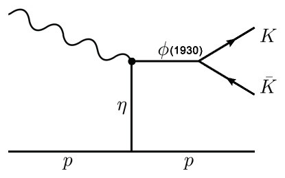
The putative state $\phi(1930)$ is quite broad, thus making its discovery more difficult. Yet, a dedicated search by using partial wave analysis could reveal the existence of this state. In general, the very promising GlueX [77, 78, 79] and CLAS12 [80] experiments take place in the near future. The process in Fig. 1

$$\gamma+p\rightarrow K^{+}+K^{-}+p\text{ , }\gamma+p\rightarrow K^{0}+\bar{K}^{0}+p$$ (72)

is an example of a process that can be studied at GlueX and CLAS12. Quite remarkably, each mesonic vertex is contained in the present paper: $\phi(1930)\gamma\eta$ and $\phi(1930)KK$. An important outlook of the present work is a dedicated study of this reaction. For the baryonic part, one can use a well defined hadronic model containing baryons and their interactions with mesons (in particular, the coupling of the nucleons to the $\eta$ meson is necessary), as for instance the extended Linear Sigma Model (eLSM) based on the mirror assignment presented in Refs. [81, 82, 83]. The analogous diagram in which $\phi(1930)$ couples to $K^{\ast}(892)K$

$$\gamma+p\rightarrow K^{\ast+}(892)+K^{-}+p\rightarrow K^{+}+K^{-}+\pi^{0}+p\text{ ,}$$ (73)

also takes place (together with analogous isospin related reactions) and should be studied in the same context.

Figure 1: Feynman diagram for the process of Eq. (72).

Other experiments are important as well. In principle, the resonance $\phi(1930)$ should also be contained in the data of BABAR [84], in which the reaction $e^{+}e^{-}\rightarrow K^{+}K^{-}$ was studied. Namely, in this reaction all the vector mesons $\rho^{0}(1450),$ $\omega(1420),$ $\phi(1680),$ $\rho^{0}(1700),\omega(1650),\phi(???)\equiv\phi(1930)$ enter and an interference of different amplitudes takes place (for a recent analysis, see Ref. [85] and refs. therein). Similarly, BESIII can also study a similar reaction, but typically this experiment focussed on the range of energy above 2 GeV.

In the future, PANDA will be a leading experiment for spectroscopy [86]. While the energy in the center of mass will be too high to create excited vector mesons in a fusion process, it will be well possible to produce excited vector mesons together with light mesons (such as pions and kaons).

On the theoretical side, we enumerated the possible straightforward improvements of our approach: the systematic inclusion of large-$N_{c}$ and flavour-symmetry violating terms. With new and more precise data, this study can be easily performed. A further outlook consists in the extension of the model by using chiral symmetry. Here, it was not needed because we did not link the excited vector mesons to chiral partners. For instance, the chiral partners of the orbitally excited vector mesons are the rather well-known pseudovector mesons {$b_{1}(1235),$ $K_{1,B},$ $h_{1}(1170),$ $h_{1}(1380)$} (for the corresponding mathematical set-up, see Ref. [87]). Chiral symmetry can help to relate the decays of this nonet to the decays of {$\rho(1700),$ $K^{\ast}(1680),$ $\omega(1650),$ $\phi(???)\equiv\phi(1930)$}. The same extension to radially excited vector mesons is more difficult because the corresponding chiral partners, a nonet of excited axial-vector states, has not been yet experimentally discovered.

In conclusions, the theoretical and experimental study of the two nonets of excited vector mesons is an interesting subject of low-energy spectroscopy. While the qualitative picture seems clear, further measurements, with special attention on radiative decays, are needed to fully establish the nature of these states. Moreover, the discovery of $\phi(1930)$ would represent a nice confirmation of the quark-antiquark picture also for excited states in the low-energy domain.

Appendix A Extended form of the Lagrangian

In this Appendix we present the extended expressions of the Lagrangian introduced in Sec. 2.2, Eq. (6).

The Lagrangian terms of our model $\mathcal{L}_{iPP}$ with $i=E,D$ presented in Sec. 2, Eq. (7), are given by:

$$\mathcal{L}_{iPP} =ig_{iPP}\;\text{Tr}\big{[}[\partial^{\mu}P,V_{i,\mu}]P\big{]}$$ (74)

$$=\frac{ig_{iPP}}{4}\;\Bigl{\{}{K^{*}_{\mu}}^{0}\Big{(}(\partial^{\mu}\overline{K}^{0})\pi^{0}-\overline{K}^{0}(\partial^{\mu}\pi^{0})-\sqrt{2}(\partial^{\mu}K^{-})\pi^{+}+\sqrt{2}K^{-}(\partial^{\mu}\pi^{+})$$

$$+(\partial^{\mu}\eta_{N})\overline{K}^{0}-\eta_{N}(\partial^{\mu}\overline{K}^{0})+\sqrt{2}\eta_{S}(\partial^{\mu}\overline{K}^{0})-\sqrt{2}(\partial^{\mu}\eta_{S})\overline{K}^{0}\Big{)}$$

$$+{\overline{K}^{*}_{\mu}}^{0}\Big{(}K^{0}(\partial^{\mu}\pi^{0})-(\partial^{\mu}K^{0})\pi^{0}-\sqrt{2}K^{+}(\partial^{\mu}\pi^{-})+\sqrt{2}(\partial^{\mu}K^{+})\pi^{-}$$

$$+\eta_{N}(\partial^{\mu}K^{0})-(\partial^{\mu}\eta_{N})K^{0}-\sqrt{2}\eta_{S}(\partial^{\mu}K^{0})+\sqrt{2}(\partial^{\mu}\eta_{S})K^{0}\Big{)}$$

$$+{K^{*}_{\mu}}^{-}\Big{(}(\partial^{\mu}K^{+})\pi^{0}-K^{+}(\partial^{\mu}\pi^{0})-\sqrt{2}K^{0}(\partial^{\mu}\pi^{+})+\sqrt{2}(\partial^{\mu}K^{0})\pi^{+}$$

$$+\eta_{N}(\partial^{\mu}K^{+})-(\partial^{\mu}\eta_{N})K^{+}-\sqrt{2}\eta_{S}(\partial^{\mu}K^{+})+\sqrt{2}(\partial^{\mu}\eta_{S})K^{+}\Big{)}$$

$$+{K^{*}_{\mu}}^{+}\Big{(}K^{-}(\partial^{\mu}\pi^{0})-(\partial^{\mu}K^{-})\pi^{0}-\sqrt{2}(\partial^{\mu}\overline{K}^{0})\pi^{-}+\sqrt{2}\overline{K}^{0}(\partial^{\mu}\pi^{-})$$

$$+(\partial^{\mu}\eta_{N})K^{-}-\eta_{N}(\partial^{\mu}K^{-})+\sqrt{2}\eta_{S}(\partial^{\mu}K^{-})-\sqrt{2}(\partial^{\mu}\eta_{S})K^{-}\Big{)}$$

$$+\rho^{0}_{\mu}\Big{(}\overline{K}^{0}(\partial^{\mu}K^{0})-(\partial^{\mu}\overline{K}^{0})K^{0}+K^{+}(\partial^{\mu}K^{-})-(\partial^{\mu}K^{+})K^{-}+2\pi^{+}(\partial^{\mu}\pi^{-})-2(\partial^{\mu}\pi^{+})\pi^{-}\Big{)}$$

$$+\rho^{-}_{\mu}\Big{(}\sqrt{2}K^{+}(\partial^{\mu}\overline{K}^{0})-\sqrt{2}(\partial^{\mu}K^{+})\overline{K}^{0}+2\pi^{0}(\partial^{\mu}\pi^{+})-2(\partial^{\mu}\pi^{0})\pi^{+}\Big{)}$$

$$+\rho^{+}_{\mu}\Big{(}\sqrt{2}K^{0}(\partial^{\mu}K^{-})-\sqrt{2}(\partial^{\mu}K^{0})K^{-}+2(\partial^{\mu}\pi^{0})\pi^{-}-2\pi^{0}(\partial^{\mu}\pi^{-})\Big{)}$$

$$+\omega\Big{(}K^{0}(\partial^{\mu}\overline{K}^{0})-(\partial^{\mu}K^{0})\overline{K}^{0}+K^{+}(\partial^{\mu}K^{-})-(\partial^{\mu}K^{+})K^{-}\Big{)}$$

$$+\sqrt{2}\phi\Big{(}(\partial^{\mu}K^{0})\overline{K}^{0}-K^{0}(\partial^{\mu}\overline{K}^{0})-K^{+}(\partial^{\mu}K^{-})+(\partial^{\mu}K^{+})K^{-}\Big{)}\Bigr{\}}.$$

We recall that for $i=E$ the states correspond to $\{\rho,K^{\ast},\phi,\omega\}=${$\rho(1450),$ $K^{\ast}(1410),$ $\omega(1420),$ $\phi(1680)$} and for $i=D$ to $\{\rho,K^{\ast},\phi,\omega\}=${$\rho(1700),$ $K^{\ast}(1680),$ $\omega(1650)$, $\phi(1930)$}.

The Lagrangian terms of our model $\mathcal{L}_{iVP}$ with $i=E,D$ presented in Sec. 2, Eq. (8), are given by:

$$\mathcal{L}_{iVP} =g_{iVP}\;\text{Tr}\big{(}\tilde{V}^{\mu\nu}_{i}\{V_{\mu\nu},P\}\big{)}=2g_{iVP}\;\epsilon^{\mu\nu\alpha\beta}\;\text{Tr}\big{(}(\partial_{\alpha}V_{i,\beta})\{(\partial_{\mu}V_{\nu}),P\}\big{)}$$ (75)

$$=\frac{g_{iVP}}{2}\epsilon^{\mu\nu\alpha\beta}\;\Bigl{\{}(\partial_{\alpha}\rho_{i,\beta}^{0})\Big{(}2\pi^{0}(\partial_{\mu}\omega_{\nu})+2\eta_{N}(\partial_{\mu}\rho_{\nu}^{0})-\overline{K}^{0}(\partial_{\mu}{K^{*}_{\nu}}^{0})-K^{0}(\partial_{\mu}{\overline{K}^{*}_{\nu}}^{0})+K^{+}(\partial_{\mu}{K^{*}_{\nu}}^{-})+K^{-}(\partial_{\mu}{K^{*}_{\nu}}^{+})\Big{)}$$

$$+\sqrt{2}(\partial_{\alpha}\rho_{i,\beta}^{-})\Big{(}\sqrt{2}\pi^{+}(\partial_{\mu}\omega_{\nu})+\sqrt{2}\eta_{N}(\partial_{\mu}\rho^{+}_{\nu})+K^{+}(\partial_{\mu}{\overline{K}^{*}_{\nu}}^{0})+\overline{K}^{0}(\partial_{\mu}{K^{*}_{\nu}}^{+})\Big{)}$$

$$+\sqrt{2}(\partial_{\alpha}\rho_{i,\beta}^{+})\Big{(}\sqrt{2}\pi^{-}(\partial_{\mu}\omega_{\nu})+\sqrt{2}\eta_{N}(\partial_{\mu}\rho^{-}_{\nu})+K^{-}(\partial_{\mu}{K^{*}_{\nu}}^{0})+K^{0}(\partial_{\mu}{K^{*}_{\nu}}^{-})\Big{)}$$

$$+\sqrt{2}(\partial_{\alpha}\phi_{i,\beta})\Big{(}2\eta_{S}(\partial_{\mu}\phi_{\nu})+K^{0}(\partial_{\mu}{\overline{K}^{*}_{\nu}}^{0})+\overline{K}^{0}(\partial_{\mu}{K^{*}_{\nu}}^{0})+K^{+}(\partial_{\mu}{K^{*}_{\nu}}^{-})+K^{-}(\partial_{\mu}{K^{*}_{\nu}}^{+})\Big{)}$$

$$+(\partial_{\alpha}\omega_{i,\beta})\Big{(}2\pi^{0}(\partial_{\mu}\rho^{0}_{\nu})+2\pi^{+}(\partial_{\mu}\rho^{-}_{\nu})+2\pi^{-}(\partial_{\mu}\rho^{+}_{\nu})+2\eta_{N}(\partial_{\mu}\omega_{\nu})$$

$$+K^{0}(\partial_{\mu}{\overline{K}^{*}_{\nu}}^{0})+\overline{K}^{0}(\partial_{\mu}{K^{*}_{\nu}}^{0})+K^{+}(\partial_{\mu}{K^{*}_{\nu}}^{-})+K^{-}(\partial_{\mu}{K^{*}_{\nu}}^{+})\Big{)}$$

$$+(\partial_{\alpha}K^{*0}_{i,\beta})\Big{(}\overline{K}^{0}(\partial_{\mu}\omega_{\nu})-\pi^{0}(\partial_{\mu}{\overline{K}^{*}_{\nu}}^{0})+\sqrt{2}\pi^{+}(\partial_{\mu}{K^{*}_{\nu}}^{-})-\overline{K}^{0}(\partial_{\mu}\rho^{0}_{\nu})+\sqrt{2}K^{-}(\partial_{\mu}\rho^{+}_{\nu})$$

$$+\eta_{N}(\partial_{\mu}{\overline{K}^{*}_{\nu}}^{0})+\sqrt{2}\eta_{S}(\partial_{\mu}{\overline{K}^{*}_{\nu}}^{0})+\sqrt{2}\overline{K}^{0}(\partial_{\mu}\phi_{\nu})\Big{)}$$

$$+(\partial_{\alpha}\overline{K}^{*0}_{i,\beta})\Big{(}K^{0}(\partial_{\mu}\omega_{\nu})-\pi^{0}(\partial_{\mu}{K^{*}_{\nu}}^{0})+\sqrt{2}\pi^{-}(\partial_{\mu}{K^{*}_{\nu}}^{+})-K^{0}(\partial_{\mu}\rho^{0}_{\nu})+\sqrt{2}K^{+}(\partial_{\mu}\rho^{-}_{\nu})$$

$$+\eta_{N}(\partial_{\mu}{K^{*}_{\nu}}^{0})+\sqrt{2}\eta_{S}(\partial_{\mu}{K^{*}_{\nu}}^{0})+\sqrt{2}K^{0}(\partial_{\mu}\phi_{\nu})\Big{)}$$

$$+(\partial_{\alpha}K^{*-}_{i,\beta})\Big{(}K^{+}(\partial_{\mu}\omega_{\nu})+\pi^{0}(\partial_{\mu}{K^{*}_{\nu}}^{+})+\sqrt{2}\pi^{+}(\partial_{\mu}{K^{*}_{\nu}}^{0})+K^{+}(\partial_{\mu}\rho^{0}_{\nu})+\sqrt{2}K^{0}(\partial_{\mu}\rho^{+}_{\nu})$$

$$+\eta_{N}(\partial_{\mu}{K^{*}_{\nu}}^{+})+\sqrt{2}\eta_{S}(\partial_{\mu}{K^{*}_{\nu}}^{+})+\sqrt{2}K^{+}(\partial_{\mu}\phi_{\nu})\Big{)}$$

$$+(\partial_{\alpha}K^{*+}_{i,\beta})\Big{(}K^{-}(\partial_{\mu}\omega_{\nu})+\pi^{0}(\partial_{\mu}{K^{*}_{\nu}}^{-})+\sqrt{2}\pi^{-}(\partial_{\mu}{\overline{K}^{*}_{\nu}}^{0})+K^{-}(\partial_{\mu}\rho^{0}_{\nu})+\sqrt{2}\overline{K}^{0}(\partial_{\mu}\rho^{-}_{\nu})$$

$$+\eta_{N}(\partial_{\mu}{K^{*}_{\nu}}^{-})+\sqrt{2}\eta_{S}(\partial_{\mu}{K^{*}_{\nu}}^{-})+\sqrt{2}K^{-}(\partial_{\mu}\phi_{\nu})\Big{)}\Bigr{\}}.$$

We recall that for $i=E$ the states correspond to $\{\rho,K^{\ast},\phi,\omega\}=${$\rho(1450),$ $K^{\ast}(1410),$ $\omega(1420),$ $\phi(1680)$} and for $i=D$ to $\{\rho,K^{\ast},\phi,\omega\}=${$\rho(1700),$ $K^{\ast}(1680),$ $\omega(1650)$, $\phi(1930)$}.

Appendix B Coupling to the photon via VMD

Let us start from a single neutral $\rho^{0}$ meson. Its coupling to an electron-positron pair can be written down as:

$$\mathcal{L}_{\rho e^{+}e^{-}}=g_{\rho e^{+}e^{-}}\rho_{\mu}^{0}\bar{\psi}_{e}\gamma^{\mu}\psi_{e}\text{ .}$$ (76)

Then, the decay into $e^{+}e^{-}$ reads:

$$\Gamma_{\rho\rightarrow e^{+}e^{-}}=\frac{\sqrt{\frac{m_{\rho}^{2}}{4}-m_{e}^{2}}}{6\pi m_{\rho}^{2}}\left(m_{\rho}^{2}+2m_{e}^{2}\right)g_{\rho e^{+}e^{-}}^{2}\text{.}$$ (77)

The interaction (76) can be obtained in the framework of Vector Meson Dominance (according to the so-called VMD-1 of Ref. [37]) by considering from the Lagrangian

$$\mathcal{L}_{VMD,\rho}=e_{0}A_{\mu}\bar{\psi}_{e}\gamma^{\mu}\psi_{e}-\frac{e_{0}}{2g_{\rho}}\rho_{\mu\nu}^{0}F^{\mu\nu}\text{ ,}$$ (78)

where the coupling $g_{\rho}$ appears also in the decay amplitude of the process $\rho^{0}\rightarrow\pi^{+}\pi^{-}$. The $\rho^{0}$ meson first transforms to a photon, which then generates a lepton pair. As a consequence, the following relation holds:

$$g_{\rho e^{+}e^{-}}=\frac{e_{0}}{g_{\rho}}$$ (79)

In fact $\rho_{\mu\nu}^{0}F^{\mu\nu}\rightarrow 2q^{2}\rho_{\mu}^{0}A^{\mu},$ hence one gets in the corresponding amplitude (upon using the Feynman rules):

$$\frac{e_{0}}{2g_{\rho}}2q^{2}\frac{1}{q^{2}}=\frac{e_{0}}{g_{\rho}}.$$ (80)

Finally, VMD-1 implies that:

$$\Gamma_{\rho\rightarrow e^{+}e^{-}}=\frac{\sqrt{\frac{m_{\rho}^{2}}{4}-m_{e}^{2}}}{6\pi m_{\rho}^{2}}\left(m_{\rho}^{2}+2m_{e}^{2}\right)\left(\frac{e}{g_{\rho}}\right)^{2}.$$ (81)

The very same formula can be used for the decay into a muon pair:

$$\Gamma_{\rho\rightarrow\mu^{+}\mu^{-}}=\frac{\sqrt{\frac{m_{\rho}^{2}}{4}-m_{\mu}^{2}}}{6\pi m_{\rho}^{2}}\left(m_{\rho}^{2}+2m_{\mu}^{2}\right)\left(\frac{e}{g_{\rho}}\right)^{2}.$$ (82)

Moreover, also the decay of the other neutral scalar states can be obtained (straightforward changes due to different charges of quarks must be taken into account):

$$\Gamma_{\omega\rightarrow e^{+}e^{-}} =\frac{\sqrt{\frac{m_{\omega}^{2}}{4}-m_{e}^{2}}}{6\pi m_{\omega}^{2}}\left(m_{\omega}^{2}+2m_{e}^{2}\right)\left(\frac{e}{3g_{\rho}}\right)^{2}\text{ ,}$$ (83)

$$\Gamma_{\phi\rightarrow e^{+}e^{-}} =\frac{\sqrt{\frac{m_{\phi}^{2}}{4}-m_{e}^{2}}}{6\pi m_{\phi}^{2}}\left(m_{\phi}^{2}+2m_{e}^{2}\right)\left(-\frac{\sqrt{2}}{3}\frac{e}{g_{\rho}}\right)^{2}.$$ (84)

The extension of the latter two to the decays into a muon pair is straightforward.

The extension to the full nonet is then obtained by using the matrix for vector mesons introduced in Sec. 2, which we rewrite here for convenience:

$$V_{\mu}=\frac{1}{\sqrt{2}}\left(\begin{array}[c]{ccc}\frac{\omega}{\sqrt{2}}+\frac{\rho^{0}}{\sqrt{2}}&\rho^{+}&K(892)^{\ast+}\\ \rho^{-}&\frac{\omega}{\sqrt{2}}-\frac{\rho^{0}}{\sqrt{2}}&K(892)^{\ast 0}\\ K(892)^{\ast-}&\bar{K}(892)^{\ast 0}&\phi\end{array}\right)\text{ .}$$ (85)

The VMD approach reads:

$$\mathcal{L}_{VMD,full}=e_{0}A_{\mu}\bar{\psi}_{e}\gamma^{\mu}\psi_{e}-\frac{e}{g_{\rho}}F_{\mu\nu}Tr[V^{\mu\nu}Q]$$ (86)

with

$$Q=\left(\begin{array}[c]{ccc}2/3&0&0\\ 0&-1/3&0\\ 0&0&-1/3\end{array}\right)$$ (87)

Finally, the photon-meson mixing can be taken into account by performing the shift:

$$V_{\mu\nu}\rightarrow V_{\mu\nu}+\frac{e_{0}}{g_{\rho}}F_{\mu\nu}Q.$$ (88)

This is the shift that we have applied in order to determine the decay of the type $R\rightarrow\gamma P$ studied in this work. Intuitively, one has a decay chain of the type $R\rightarrow VP\rightarrow\gamma P,$ where in the second step the transition $V\rightarrow\gamma$ has taken place according to VMD.

Appendix C Errors of the coupling constants and their propagation

Let us consider the $\chi^{2}$ function $F\equiv F(x_{k}),$ where $x_{k}$ are the parameters of the theory with $k=1,...,N$ (in our cases, $F$ corresponds to Eq. (24) and to Eq. (29) respectively, and the parameters $x_{1}$ and $x_{2}$ are the coupling constants). We look for the minimum of $F$ by solving $\partial_{q}F(x_{k})=0\rightarrow x_{k}=x_{k}^{\min}.$ The Taylor expansion reads

$$F(x_{k})=F(x_{k}^{\min})+(x_{k}-x_{k}^{\min})H_{kq}(x_{q}-x_{q}^{\min})+...\text{, }H_{kq}=\left.\frac{1}{2}\frac{\partial^{2}F}{\partial x_{k}\partial x_{q}}\right|_{x_{k}=x_{k}^{\min}}$$ (89)

The matrix $H$, with elements $H_{kq}$, is the Hesse matrix of the function $F$ evaluated at the minimum. We introduce the matrix $B$ such that $BHB^{t}=D=diag\{\lambda_{1},...,\lambda_{N}\}$ and the new variables $z_{k}=B_{kq}(x_{q}-x_{q}^{\min})$ (note: $B_{kq}=\frac{\partial z_{k}}{\partial x_{q}}$). As function of $z_{k}$, we get

$$F\equiv F(z_{k})=F(x_{k}^{\min})+z_{k}^{2}\lambda_{k}+...\text{ ,}$$ (90)

therefore the error of $z_{k}$ is given by $\delta z_{k}=1/\sqrt{\lambda_{k}}$ (increment of $1$ of the $\chi^{2}$). Next, let us consider an arbitrary function of the parameters, $G\equiv G(x_{k})$, which represents some physical quantity of interest (in our examples, it can be a decay width or a ratio of decay widths). The physical value of $G$ is clearly given by $G(x_{k}^{\min}).$ Its error is evaluated w.r.t. the (mutually independent) parameters $z_{k}$:

$$\delta G=\sqrt{\left(\left.\frac{\partial G}{\partial z_{k}}\right|_{z_{k}=0}\delta z_{k}\right)^{2}}\text{ ,}$$ (91)

where

$$\left.\frac{\partial G}{\partial z_{k}}\right|_{z_{k}=0}=\left.\frac{\partial G}{\partial x_{q}}\right|_{x_{k}=x_{k}^{\min}}B_{qk}^{t}=\left.\frac{\partial G}{\partial x_{q}}\right|_{x_{k}=x_{k}^{\min}}B_{kq}\text{ .}$$ (92)

The errors of the parameters $x_{r}$ is calculated by setting $G=x_{r},$ out of which (upon using $\frac{\partial x_{r}}{\partial z_{k}}=B_{rk}^{t}=B_{kr}$):

$$\delta x_{r}=\sqrt{\left(B_{kr}\delta z_{k}\right)^{2}}=\sqrt{H_{rr}^{-1}}.$$ (93)

(For the last equality we used $H^{-1}=B^{t}D^{-1}B\rightarrow H_{rr}^{-1}=B_{rq}^{t}D_{qk}^{-1}B_{kr}=B_{rk}^{t}\delta z_{k}^{2}B_{kr}=B_{kr}^{2}\delta z_{k}^{2}$). In this way we evaluated the parameter errors in Sec. 3.1. It is also interesting to mention that the naive evaluation of the error of $G$ as

$$\delta G^{naive}=\sqrt{\left(\left.\frac{\partial G}{\partial x_{k}}\right|_{x_{k}=x_{k}^{\min}}\delta x_{k}\right)^{2}}$$ (94)

is in general not correct (typically, it is an overestimation of the error $\delta G$).

Finally, we turn to our concrete examples. For the nonet of radially excited vector states, we identify $x_{1}=g_{EPP}$ and $x_{2}=g_{EVP},$ and $F$ is given by Eq. (24). Here, the Hesse matrix is from the very beginning diagonal. Than, in this particular case $\delta G^{naive}=\delta G,$ hence the error of a certain quantity $G(g_{EPP}$,$g_{EVP})$ reads:

$$\delta G=\sqrt{\left(\left.\frac{\partial G}{\partial g_{EPP}}\right|_{\min}\delta g_{EPP}\right)^{2}+\left(\left.\frac{\partial G}{\partial g_{EVP}}\right|_{\min}\delta g_{EVP}\right)^{2}}$$ (95)

where ‘min’ refers to the values of Eq. (25). In this way all the errors of the quantities of Sec. 3.2 were evaluated.

For what concerns the nonet of orbitally excited vector states, we set $x_{1}=g_{DPP}$ and $x_{2}=g_{DVP}$ and use $F$ from Eq. (29). While for the decays in Tables 9, 10, and 11 (which involve only one of the two coupling constants) the naive procedure would still be valid, this is not true in general and the diagonalization is necessary. For instance, for the ratios of coupling constants (entering in various decay ratios studied in Sec. 3.3), one sets $G=g_{DPP}^{2}/g_{DVP}^{2}$ . The central value reads $5.4$ and the corresponding error is $\delta G=1.8$, whereas $\delta G^{naive}=2.7$ would be an overestimation.

In this work, we have limited our evaluation of the errors to the couplings discussed above because they represent the largest source of inderterminacy. Yet, as mentioned in the text, other error sources (not included here) exist, such as masses and flavour-breaking and large-$N_{c}$ suppressed terms.

References

- [1] C. Patrignani et al. (Particle Data Group), Chin. Phys. C, 40, 100001 (2016).
- [2] S. Godfrey and N. Isgur, “Mesons in a Relativized Quark Model with Chromodynamics,” Phys. Rev. D 32 (1985) 189. doi:10.1103/PhysRevD.32.189
- [3] C. Amsler and N. A. Tornqvist, “Mesons beyond the naive quark model,” Phys. Rept. 389 (2004) 61. doi:10.1016/j.physrep.2003.09.003
- [4] E. Klempt and A. Zaitsev, “Glueballs, Hybrids, Multiquarks. Experimental facts versus QCD inspired concepts,” Phys. Rept. 454 (2007) 1 doi:10.1016/j.physrep.2007.07.006 [arXiv:0708.4016 [hep-ph]].
- [5] J. R. Pelaez, “From controversy to precision on the sigma meson: a review on the status of the non-ordinary resonance,” Phys. Rept. 658 (2016) 1 doi:10.1016/j.physrep.2016.09.001 [arXiv:1510.00653 [hep-ph]].
- [6] W. Ochs, “The Status of Glueballs,” J. Phys. G 40 (2013) 043001 doi:10.1088/0954-3899/40/4/043001 [arXiv:1301.5183 [hep-ph]].
- [7] H. X. Chen, W. Chen, X. Liu and S. L. Zhu, “The hidden-charm pentaquark and tetraquark states,” Phys. Rept. 639 (2016) 1 doi:10.1016/j.physrep.2016.05.004 [arXiv:1601.02092 [hep-ph]].
- [8] S. Capstick and N. Isgur, “Baryons in a Relativized Quark Model with Chromodynamics,” Phys. Rev. D 34 (1986) 2809 [AIP Conf. Proc. 132 (1985) 267]. doi:10.1103/PhysRevD.34.2809, 10.1063/1.35361
- [9] R. Aaij et al. [LHCb Collaboration], “Observation of Resonances Consistent with Pentaquark States in Decays,” Phys. Rev. Lett. 115 (2015) 072001 doi:10.1103/PhysRevLett.115.072001 [arXiv:1507.03414 [hep-ex]].
- [10] Quark model, Standard Model and related topics, Reviews, Tables and Plots of the PDG [1].
- [11] S. S. Afonin and I. V. Pusenkov, “Universal description of radially excited heavy and light vector mesons,” Phys. Rev. D 90 (2014) no.9, 094020 doi:10.1103/PhysRevD.90.094020 [arXiv:1411.2390 [hep-ph]].
- [12] F. Caporale and I. P. Ivanov, “Production of orbitally excited vector mesons in diffractive DIS,” Phys. Lett. B 622 (2005) 55 doi:10.1016/j.physletb.2005.06.075 [hep-ph/0505266].
- [13] A. M. Badalian and B. L. G. Bakker, “Radial Regge trajectories and leptonic widths of the isovector mesons,” Phys. Rev. D 93 (2016) no.7, 074034 doi:10.1103/PhysRevD.93.074034 [arXiv:1603.04725 [hep-ph]].
- [14] S. Coito, G. Rupp and E. van Beveren, “Unquenched quark-model calculation of excited resonances and P-wave phase shifts,” Bled Workshops Phys. 16 (2015) no.1, [arXiv:1510.00938 [hep-ph]].
- [15] G. Rupp, S. Coito and E. van Beveren, “Unquenching the meson spectrum: a model study of excited resonances,” Acta Phys. Polon. Supp. 9 (2016) 653 doi:10.5506/APhysPolBSupp.9.653 [arXiv:1605.04260 [hep-ph]].
- [16] D. Parganlija and F. Giacosa, “Excited Scalar and Pseudoscalar Mesons in the Extended Linear Sigma Model,” arXiv:1612.09218 [hep-ph], to appear in EPJ C.
- [17] A. Pich, “Chiral perturbation theory,” Rept. Prog. Phys. 58 (1995) 563 doi:10.1088/0034-4885/58/6/001 [hep-ph/9502366].
- [18] S. Scherer, “Introduction to chiral perturbation theory,” Adv. Nucl. Phys. 27 (2003) 277 [hep-ph/0210398].
- [19] S. Gasiorowicz and D. A. Geffen, “Effective Lagrangians and field algebras with chiral symmetry,” Rev. Mod. Phys. 41 (1969) 531. doi:10.1103/RevModPhys.41.531.
- [20] C. Rosenzweig, J. Schechter and C. G. Trahern, “Is the Effective Lagrangian for QCD a Sigma Model?,” Phys. Rev. D 21 (1980) 3388. doi:10.1103/PhysRevD.21.3388.
- [21] A. H. Fariborz, R. Jora and J. Schechter, “Toy model for two chiral nonets,” Phys. Rev. D 72 (2005) 034001 doi:10.1103/PhysRevD.72.034001 [hep-ph/0506170].
- [22] D. Parganlija, P. Kovacs, G. Wolf, F. Giacosa and D. H. Rischke, “Meson vacuum phenomenology in a three-flavor linear sigma model with (axial-)vector mesons,” Phys. Rev. D 87 (2013) no.1, 014011 doi:10.1103/PhysRevD.87.014011 [arXiv:1208.0585 [hep-ph]].
- [23] S. Janowski, F. Giacosa and D. H. Rischke, “Is f0(1710) a glueball?,” Phys. Rev. D 90 (2014) no.11, 114005 doi:10.1103/PhysRevD.90.114005 [arXiv:1408.4921 [hep-ph]].
- [24] R. Alkofer and L. von Smekal, “The Infrared behavior of QCD Green’s functions: Confinement dynamical symmetry breaking, and hadrons as relativistic bound states,” Phys. Rept. 353 (2001) 281 doi:10.1016/S0370-1573(01)00010-2 [hep-ph/0007355].
- [25] G. Eichmann, H. Sanchis-Alepuz, R. Williams, R. Alkofer and C. S. Fischer, “Baryons as relativistic three-quark bound states,” Prog. Part. Nucl. Phys. 91 (2016) 1 doi:10.1016/j.ppnp.2016.07.001 [arXiv:1606.09602 [hep-ph]].
- [26] F. Giacosa, T. Gutsche, V. E. Lyubovitskij and A. Faessler, “Decays of tensor mesons and the tensor glueball in an effective field approach,” Phys. Rev. D 72 (2005) 114021 doi:10.1103/PhysRevD.72.114021 [hep-ph/0511171].
- [27] F. Divotgey, L. Olbrich and F. Giacosa, “Phenomenology of axial-vector and pseudovector mesons: decays and mixing in the kaonic sector,” Eur. Phys. J. A 49 (2013) 135 doi:10.1140/epja/i2013-13135-3 [arXiv:1306.1193 [hep-ph]].
- [28] A. Koenigstein and F. Giacosa, “Phenomenology of pseudotensor mesons and the pseudotensor glueball,” Eur. Phys. J. A 52 (2016) no.12, 356 doi:10.1140/epja/i2016-16356-x [arXiv:1608.08777 [hep-ph]].
- [29] F. Giacosa, T. Gutsche, V. E. Lyubovitskij and A. Faessler, “Scalar nonet quarkonia and the scalar glueball: Mixing and decays in an effective chiral approach,” Phys. Rev. D 72 (2005) 094006 doi:10.1103/PhysRevD.72.094006 [hep-ph/0509247].
- [30] F. Giacosa, T. Gutsche, V. E. Lyubovitskij and A. Faessler, “Scalar meson and glueball decays within a effective chiral approach,” Phys. Lett. B 622 (2005) 277 doi:10.1016/j.physletb.2005.07.016 [hep-ph/0504033].
- [31] G. Amelino-Camelia et al., “Physics with the KLOE-2 experiment at the upgraded DANE,” Eur. Phys. J. C 68 (2010) 619 doi:10.1140/epjc/s10052-010-1351-1 [arXiv:1003.3868 [hep-ex]].
- [32] T. Feldmann, P. Kroll and B. Stech, “Mixing and decay constants of pseudoscalar mesons,” Phys. Rev. D 58 (1998) 114006 doi:10.1103/PhysRevD.58.114006 [hep-ph/9802409].
- [33] S. D. Bass and A. W. Thomas, “eta bound states in nuclei: A Probe of flavor-singlet dynamics,” Phys. Lett. B 634 (2006) 368 doi:10.1016/j.physletb.2006.01.071 [hep-ph/0507024].
- [34] S. Prelovsek, L. Leskovec, C. B. Lang and D. Mohler, “ scattering and the K* decay width from lattice QCD,” Phys. Rev. D 88 (2013) no.5, 054508 doi:10.1103/PhysRevD.88.054508 [arXiv:1307.0736 [hep-lat]].
- [35] J. J. Dudek, R. G. Edwards, B. Joo, M. J. Peardon, D. G. Richards and C. E. Thomas, “Isoscalar meson spectroscopy from lattice QCD,” Phys. Rev. D 83 (2011) 111502 doi:10.1103/PhysRevD.83.111502 [arXiv:1102.4299 [hep-lat]];
- [36] J. J. Dudek et al. [Hadron Spectrum Collaboration], “Toward the excited isoscalar meson spectrum from lattice QCD,” Phys. Rev. D 88 (2013) no.9, 094505 doi:10.1103/PhysRevD.88.094505 [arXiv:1309.2608 [hep-lat]].
- [37] H. B. O’Connell, B. C. Pearce, A. W. Thomas and A. G. Williams, “ mixing, vector meson dominance and the pion form-factor,” Prog. Part. Nucl. Phys. 39 (1997) 201 doi:10.1016/S0146-6410(97)00044-6 [hep-ph/9501251].
- [38] G. ’t Hooft, “A Planar Diagram Theory for Strong Interactions,” Nucl. Phys. B 72 (1974) 461. doi:10.1016/0550-3213(74)90154-0
- [39] E. Witten, “Baryons in the 1/n Expansion,” Nucl. Phys. B 160 (1979) 57. doi:10.1016/0550-3213(79)90232-3
- [40] F. Giacosa and G. Pagliara, “On the spectral functions of scalar mesons,” Phys. Rev. C 76 (2007) 065204 doi:10.1103/PhysRevC.76.065204 [arXiv:0707.3594 [hep-ph]].
- [41] M. Boglione and M. R. Pennington, “Dynamical generation of scalar mesons,” Phys. Rev. D 65 (2002) 114010 doi:10.1103/PhysRevD.65.114010 [hep-ph/0203149].
- [42] T. Wolkanowski, F. Giacosa and D. H. Rischke, “ revisited,” Phys. Rev. D 93 (2016) no.1, 014002 doi:10.1103/PhysRevD.93.014002 [arXiv:1508.00372 [hep-ph]].
- [43] T. Wolkanowski, M. Soltysiak and F. Giacosa, “ as a companion pole of ,” Nucl. Phys. B 909 (2016) 418 doi:10.1016/j.nuclphysb.2016.05.025 [arXiv:1512.01071 [hep-ph]].
- [44] M. Soltysiak, T. Wolkanowski and F. Giacosa, “Large- pole trajectories of the vector kaon and of the scalar kaons and ,” Acta Phys. Polon. Supp. 9 (2016) 321 doi:10.5506/APhysPolBSupp.9.321 [arXiv:1604.01636 [hep-ph]].
-
[45]
D. Aston et al., “A Study of K- pi+ Scattering in
the Reaction K- p —¿ K- pi+ n at 11-GeV/c,” Nucl. Phys. B 296
(1988) 493.
[46]
A. B. Clegg and A. Donnachie, “Higher vector meson states
produced in electron - positron annihilation,” Z. Phys. C 62
(1994) 455. doi:10.1007/BF01555905
[47]
V. M. Aulchenko et al. [SND Collaboration],
“Measurement of the cross section in the
center-of-mass energy range 1.22-2.00 GeV with the SND detector at the
VEPP-2000 collider,” Phys. Rev. D 91 (2015) no.5, 052013
doi:10.1103/PhysRevD.91.052013 [arXiv:1412.1971 [hep-ex]].
[48]
A. Donnachie and A. B. Clegg, “The Decays of the
rho-prime(1) and omega-prime(1) mesons,” Z. Phys. C 51 (1991) 689.
doi:10.1007/BF01565597
[49]
S. Fukui et al., “Study of omega pi0 system in the
pi- p charge exchange reaction at 8.95-GeV/c,” Phys. Lett. B 257
(1991) 241. doi:10.1016/0370-2693(91)90888-W
- [50] P. Bydžovský, R. Kaminski and V. Nazari, “Dispersive analysis of the -, -, -, and -wave amplitudes,” Phys. Rev. D 94 (2016) no.11, 116013 doi:10.1103/PhysRevD.94.116013 [arXiv:1611.10070 [hep-ph]]. V. Nazari, PhD Thesis, krakow, 2016.
[51]
D. Aston et al., “Observation of Two Nonleading
Strangeness 1 Vector Mesons,” Phys. Lett. 149B (1984) 258.
doi:10.1016/0370-2693(84)91595-8
[52]
M. N. Achasov et al., “Measurement of the
cross section below GeV,”
Phys. Rev. D 94 (2016) no.9, 092002 doi:10.1103/PhysRevD.94.092002
[arXiv:1607.00371 [hep-ex]].
[53]
V.M. Aulchenko et al. “Study of the
process in the energy range
GeV,” J.Exp.Theor.Phys. 121 (2015) no.1, 27-34,
Zh.Eksp.Teor.Fiz. 148 (2015) no.1, 34-41
[54]
J. Buon, D. Bisello, J. C. Bizot, A. Cordier, B. Delcourt,
F. Mane and J. Layssac, “Interpretation of Dm1 Results on
Annihilation Into Exclusive Channels Between 1.4-GeV and 1.9-GeV With a
Model,”
Phys. Lett. 118B (1982) 221.
doi:10.1016/0370-2693(82)90632-3
[55]
B. Aubert et al. [BaBar Collaboration],
“Measurements of ,
and cross- sections using initial state radiation
events,” Phys. Rev. D 77 (2008) 092002
doi:10.1103/PhysRevD.77.092002 [arXiv:0710.4451 [hep-ex]].
[56]
R. R. Akhmetshin et al. [CMD-2
Collaboration], “Study of the process e+ e- —¿ eta gamma in center-of-mass
energy range 600-MeV to 1380-MeV at CMD-2,” Phys. Lett. B 509
(2001) 217 doi:10.1016/S0370-2693(01)00567-6 [hep-ex/0103043].
[57]
B. Diekmann, “Spectroscopy of Mesons Containing Light
Quarks (, , ) or Gluons,” Phys. Rept. 159 (1988) 99.
doi:10.1016/0370-1573(88)90062-2
[58]
L. M. Kurdadze et al., “Measuring Of Pion
Form-factor Within The Region S**(1/2) From 640-mev To 1400-mev,” JETP
Lett. 37 (1983) 733 [Pisma Zh. Eksp. Teor. Fiz. 37
(1983) 613].
[59]
R. R. Akhmetshin et al. [CMD-2 Collaboration],
“Study of the processes e+ e- —¿ eta gamma, pi0 gamma —¿ 3 gamma in the
c.m. energy range 600-MeV to 1380-MeV at CMD-2,” Phys. Lett. B 605
(2005) 26 doi:10.1016/j.physletb.2004.11.020 [hep-ex/0409030].
[60]
V. K. Henner, T. S. Belozerova, V. G. Solovev and
P. G. Frick, “Application of wavelet analysis to the spectrum of omega’
states and ratio R(e+ e-),” Eur. Phys. J. C 26 (2002) 3.
doi:10.1140/epjc/s2002-01060-y
- [61] M. N. Achasov et al., “Study of the process in the energy region below 0.98-GeV,” Phys. Rev. D 68 (2003) 052006 doi:10.1103/PhysRevD.68.052006 [hep-ex/0305049].
- [62] A. Alavi-Harati et al. [KTeV Collaboration], “Search for the K(L) —¿ pi0 pi0 e+ e- decay in the KTeV experiment,” Phys. Rev. Lett. 89 (2002) 211801 doi:10.1103/PhysRevLett.89.211801 [hep-ex/0210056].
- [63] M. N. Achasov et al., “Study of the process in the center-of-mass energy range 1.07–2.00 GeV,” Phys. Rev. D 90 (2014) no.3, 032002 doi:10.1103/PhysRevD.90.032002 [arXiv:1312.7078 [hep-ex]].
- [64] H. Becker et al. [CERN-Cracow-Munich Collaboration], “A Model Independent Partial Wave Analysis of the pi+ pi- System Produced at Low Four Momentum Transfer in the Reaction pi- p (Polarized) — pi+ pi- n at 17.2-GeV/c,” Nucl. Phys. B 151 (1979) 46. doi:10.1016/0550-3213(79)90426-7
[65]
A. D. Martin and M. R. Pennington, “How Imposing
Analyticity on a pi pi Phase Shift Analysis Can Reveal New Solutions, Explore
Experimental Structures and Investigate the Possibility of New Resonances,”
Annals Phys. 114 (1978) 1. doi:10.1016/0003-4916(78)90262-2
[66]
C. D. Froggatt and J. L. Petersen, “Phase Shift Analysis
of pi+ pi- Scattering Between 1.0-GeV and 1.8-GeV Based on Fixed Momentum
Transfer Analyticity. 2.,” Nucl. Phys. B 129 (1977) 89.
doi:10.1016/0550-3213(77)90021-9
[67]
B. Hyams et al., “ Phase Shift Analysis
from 600-MeV to 1900-MeV,” Nucl. Phys. B 64 (1973) 134.
doi:10.1016/0550-3213(73)90618-4
[68]
A. Cordier, D. Bisello, J. C. Bizot, J. Buon,
B. Delcourt, L. Fayard and F. Mane, “Study of the Reaction in the 1.4-GeV to 2.18-GeV Energy
Range,” Phys. Lett. 109B (1982) 129.
doi:10.1016/0370-2693(82)90478-6; B. Delcourt et al., “ Annihilation at DCI with the Magnetic Detector DM1 for GeV,” eConf C 810824 (1981) 205.
[69]
D. Aston et al. [Bonn-CERN-Ecole
Poly-Glasgow-Lancaster-Manchester-Orsay-Paris-Rutherford-Sheffield
Collaboration], “Observation of the prime (1600) in the Channel
,” Phys. Lett. 92B (1980) 215.
doi:10.1016/0370-2693(80)90340-8
- [70] T. E. Coan et al. [CLEO Collaboration], “Wess-Zumino current and the structure of the decay tau- — K- K+ pi- nu(tau),” Phys. Rev. Lett. 92 (2004) 232001 doi:10.1103/PhysRevLett.92.232001 [hep-ex/0401005].
[71]
J. C. Bizot et al., “Observation
of a vector meson in annihilation at
DCI,” AIP Conf. Proc. 68 (1981) 546.
doi:10.1063/1.32532
[72]
B. Delcourt, D. Bisello, J. C. Bizot, J. Buon, A. Cordier
and F. Mane, “Study of the Reactions , ,
and for Total Energy Ranges Between 1.4-GeV and
2.18-GeV,” Phys. Lett. 113B (1982) 93 Erratum:
[Phys. Lett. 115B (1982) 503].
doi:10.1016/0370-2693(82)90116-2
- [73] A. Donnachie and A. B. Clegg, “ in Diffractive Photoproduction and Annihilation,” Z. Phys. C 34 (1987) 257. doi:10.1007/BF01566768
[74]
A. Antonelli et al. [DM2 Collaboration],
“Measurement of the Reaction in the
Center-of-mass Energy Interval 1350-MeV to 2400-MeV,” Phys. Lett. B
212 (1988) 133. doi:10.1016/0370-2693(88)91250-6
[75]
D. Aston et al., “The Strange Meson Resonances
Observed in the Reaction at
11-GeV/,” Nucl. Phys. B 292 (1987) 693.
doi:10.1016/0550-3213(87)90665-1
- [76] B. Aubert et al. [BaBar Collaboration], Phys. Rev. D 73 (2006) 052003 doi:10.1103/PhysRevD.73.052003 [hep-ex/0602006].
- [77] H. Al Ghoul et al. [GlueX Collaboration], “First Results from The GlueX Experiment,” AIP Conf. Proc. 1735 (2016) 020001 doi:10.1063/1.4949369 [arXiv:1512.03699 [nucl-ex]].
- [78] B. Zihlmann [GlueX Collaboration], “GlueX a new facility to search for gluonic degrees of freedom in mesons,” AIP Conf. Proc. 1257 (2010) 116. doi:10.1063/1.3483306.
- [79] M. Shepherd, “GlueX at Jefferson Lab: a search for exotic states of matter in photon-proton collisions,” PoS Bormio 2014 (2014) 004.
- [80] A. Rizzo [CLAS Collaboration], “The meson spectroscopy program with CLAS12 at Jefferson Laboratory,” PoS CD 15 (2016) 060.
- [81] S. Gallas, F. Giacosa and D. H. Rischke, “Vacuum phenomenology of the chiral partner of the nucleon in a linear sigma model with vector mesons,” Phys. Rev. D 82 (2010) 014004 doi:10.1103/PhysRevD.82.014004 [arXiv:0907.5084 [hep-ph]].
- [82] L. Olbrich, M. Zétényi, F. Giacosa and D. H. Rischke, “Three-flavor chiral effective model with four baryonic multiplets within the mirror assignment,” Phys. Rev. D 93 (2016) no.3, 034021 doi:10.1103/PhysRevD.93.034021 [arXiv:1511.05035 [hep-ph]].
- [83] L. Olbrich, M. Zétényi, F. Giacosa and D. H. Rischke, “Influence of the axial anomaly on the decay ,” arXiv:1708.01061 [hep-ph].
- [84] J. P. Lees et al. [BaBar Collaboration], “Precision measurement of the cross section with the initial-state radiation method at BABAR,” Phys. Rev. D 88 (2013) no.3, 032013 doi:10.1103/PhysRevD.88.032013 [arXiv:1306.3600 [hep-ex]].
- [85] V. Sauli, “Hadronic vacuum polarization in process bellow 3 GeV,” arXiv:1704.01887 [hep-ph].
- [86] M. F. M. Lutz et al. [ PANDA Collaboration ], “Physics Performance Report for PANDA: Strong Interaction Studies with Antiprotons,” arXiv:0903.3905 [hep-ex]].
- [87] F. Giacosa, J. Sammet and S. Janowski, “Decays of the vector glueball,” Phys. Rev. D 95 (2017) no.11, 114004 doi:10.1103/PhysRevD.95.114004 [arXiv:1607.03640 [hep-ph]].