Exact description of paramagnetic and ferromagnetic phases of an Ising model on a third-order Cayley tree

Abstract.

In this paper we analytically study the recurrence equations of an Ising model with three competing interactions on a Cayley tree of order three. We exactly describe paramagnetic and ferromagnetic phases of the Ising model. We obtain some rigorous results: critical temperatures and curves, number of phases, partition function. Ganikhodjaev et al. [2] have numerically studied the Ising model on a second-order Cayley tree. We compare the numerical results to exact solutions of mentioned model.
Keywords: Cayley tree, Ising model, paramagnetic phase.
PACS: 05.70.Fh; 05.70.Ce; 75.10.Hk.

1. Introduction

A phase diagram of a model with variety of transition lines and modulated phases are obtained via the presence of competing interactions in magnetic and ferroelectric systems [37]. In order to describe all phases of considered model, one iterates the recurrence relations associated to the given Hamiltonian and observes their behavior after a large number of iterations [14, 17, 36, 35]. The ANNNI (Axial Next-Nearest-Neighbor Ising) model, which consists of an Ising spin Hamiltonian on a Cayley tree, with ferromagnetic interactions on the planes, and competing ferromagnetic and antiferromagnetic interactions between nearest and next-nearest neighbors along an axial direction, is known to reproduce some features of these complex phase diagrams [10, 14, 36].

In recent times, existence and quantification of the phase diagrams after a large number of iterations of relevant recurrence equations as a way of probing ground phases of Ising model have gained much attention [2, 4, 12, 14, 18, 23, 24, 25, 28, 35, 36, 37, 38]. In generally by analyzing the regions of stability of different types of fixed points of the system of recurrent relations, many authors have plotted the phase diagrams of the model [2, 4, 12, 14, 18, 23, 26, 35, 36]. Most results of the above-mentioned works are obtained numerically. In this paper, we try to get some of these results by an analytical way by comparing the numerical results.

In [35], we numerically study Lyapunov exponent and modulated phases for the Ising system with competing interactions on an arbitrary order Cayley tree, the variation of the wavevector $q$ with temperature in the modulated phase and the Lyapunov exponent associated with the trajectory of our iterative system are studied in detail. In [3], we have analytically study the recurrence equations of an Ising model with two competing interactions on a Cayley tree of order two and obtained some exact results: critical temperatures and curves, number of phases, partition function without considering the numerical investigation. In [5] we have described the exact solution of a phase transition problem by means Gibbs measures of the Potts model on a Cayley tree of order three with competing interactions. In [1] we have constructed a class of new Gibbs measures by extending the known Gibbs measures defined on a Cayley tree of order $k_{0}$ to a Cayley tree of higher order $k>k_{0}$ for the Ising model. Nazarov and Rozikov [33] find the operator corresponding to the periodic Gibbs distributions with period two and determine the invariant subsets of this operator, which are used to describe the periodic Gibbs distributions. Here in order to obtain the periodic fixed points associated with the recurrence equations, we use the similar methods in [22, 27].

In the ref. [7], the author studies the Gibbs measures associated with Vannimenus-Ising model for compatible conditions, he has been interested in the existence of the translation-invariant Gibbs measures with respect to the compatible conditions. Our present results differ from [6, 7, 8, 31], because we have considered external magnetic field in the mentioned papers (see [9, 11]).

In the present paper, we analytically study the recurrence equations of an Ising model with three competing interactions on a three order Cayley tree. We obtain the paramagnetic, ferromagnetic and 2-period phases of the model via the related recurrence equations. We exactly describe paramagnetic phase of the Ising model. We obtain some rigorous results: critical temperatures and curves, number of phases, partition function. This model was numerically studied by Ganikhodjaev et al. [2] on semi-infinitive second-order Cayley tree.

2. Preliminary

2.1. Cayley tree

A tree is a graph which is connected and contains no circuits. In this paper, we consider an semi-infinite tree which has uniformly bounded degrees. That is, the numbers of neighbors of any vertices in this tree are uniformly bounded; we call it the uniformly bounded tree. If the root of a tree has $k$ neighboring vertices and other vertices have $k+1$ neighboring vertices, we call this type of tree a Cayley tree. It is easy to see that this type of tree is the special case of uniformly bounded tree. Cayley trees (or Bethe lattices) are simple connected undirected graphs $G=(V,E)$ ($V$ set of vertices, $E$ set of edges) with no cycles (a cycle is a closed path of different edges), i.e., they are trees [7]. Let $\Gamma^{k}=(V,L,i)$ be the uniform Cayley tree of order $k$ with a root vertex $x^{(0)}\in V$, where each vertex has $(k+1)$ neighbors with $V$ as the set of vertices and the set of edges. The notation $i$ represents the incidence function corresponding to each edge $\ell\in L$, with end points $x_{1},x_{2}\in V$. There is a distance $d(x,y)$ on $V$ the length of the minimal point from $x$ to $y$, with the assumed length of 1 for any edge (see Figure 1).

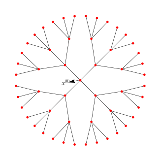
Figure 1. Cayley tree of order $k=3$

Any $k$ ($k>1$)-order Cayley tree $\Gamma^{k}$ is a weave pattern in which $(k+1)$ edges from each vertex point extend infinitely as shown in Fig. 1 ($k=3$). For the Cayley tree shown as $\Gamma^{k}=(V,\Lambda)$, $V$ denotes the corner points of the Cayley tree and $\Lambda$ denotes the set of edges. If there is an edge $\ell$ joining two vertex $x$ and $y$, it is called ”nearest neighbor” and $l=<x,y>$. The distance of $x$ and $y$, over $V$ is defined as $d(x,y)$, the shortest path between $x$ and $y$. For any given point $x^{(0)}\in V$, the set of levels according to this point is given as $V_{n}=\{x\in V|d(x,x^{(0)})\leq n\}$ and the set of edge points in $V_{n}$ is represented as $L_{n}$.

The set of all vertices with distance $n$ from the root $x^{(0)}$ is called the $n$th level of $\Gamma^{k}$ ann we denote the sphere of radius $n$ on $V$ by

$$W_{n}=\{x\in V:d(x,x^{(0)})=n\}$$

and the ball of radius $n$ by

$$V_{n}=\{x\in V:d(x,x^{(0)})\leq n\}.$$

The set of direct successors of any vertex $x\in W_{n}$ is denoted by

$$S_{k}(x)=\{y\in W_{n+1}:d(x,y)=1\}.$$

A Cayley tree $\Gamma^{k}$ of order $k\geq 1$ is an infinite tree, i.e., a graph without cycles with exactly $k+1$ edges issuing from each vertex. Let denote the Cayley tree as $\Gamma^{k}=(V,\Lambda),$ where $V$ is the set of vertices of $\Gamma^{k}$, $\Lambda$ is the set of edges of $\Gamma^{k}$.

The distance $d(x,y),x,y\in V$, on the Cayley tree $\Gamma^{k}$, is the number of edges in the shortest path from $x$ to $y$. The fixed vertex $x^{(0)}$ is called the $0$-th level and the vertices in $W_{n}$ are called the $n$-th level. For the sake of simplicity we put $|x|=d(x,x^{(0)})$, $x\in V$.

Definition 2.1.

Hereafter, we will use the following definitions for neighborhoods.

1. Two vertices $x$ and $y$, $x,y\in V$ are called nearest-neighbors (NN) if there exists an edge $l\in\Lambda$ connecting them, which is denoted by $l=<x,y>$.

2. The next-nearest-neighbor vertices $x\in W_{n}$ and $z\in W_{n+2}$ are called prolonged next-nearest-neighbors (PNNN) if $|x|\neq|y|$ and is denoted by $>x,z<$

3. The triple of vertices $x,y,z$ is called ternary prolonged next-nearest-neighbors if $x\in W_{n},y\in S(x)$ and $z\in S(y)$ ($x\in W_{n},y\in W_{n+1}$ and $z\in W_{n+2}$) for some nonnegative integer $n$ and is denoted by $>x,y,z<$.

In this paper, we will consider an Hamiltonian with competing nearest-neighbor interactions, prolonged next-nearest-neighbors (PNNN) and ternary prolonged next nearest-neighbor interactions. Therefore, we can state the Hamiltonian by

(2.1) $$H(\sigma)=-J\sum_{\begin{array}[]{l}<x,y>\\ y\in S(x)\end{array}}\sigma(x)\sigma(y)-J_{p}\sum_{\begin{array}[]{l}>x,z<\\ z\in S^{2}(x)\end{array}}\sigma(x)\sigma(z)-J_{t}\sum_{\begin{array}[]{l}>x,y,z<\\ y\in S(x)\\ z\in S(y)\end{array}}\sigma(x)\sigma(y)\sigma(z),$$

where $J,J_{p},J_{t}\in\mathbb{R}$ are coupling constants and $<x,y>$ stands for NN vertices, $>x,z<$ stands for prolonged NNN and $>x,y,z<$ stands for prolonged ternary NNN. Note that the joule, symbol $J$, is a derived unit of energy in the International System of Units.

3. Recursive equations for Partition Functions

There are several approaches to derive equation or system equations describing limiting Gibbs measure (phases) for lattice models on Cayley tree. One approach is based on properties of Markov random fields on Bethe lattices [16, 19, 29, 30]. Another approach is based on recursive equations for partition functions (for example [34]). Naturally, both approaches lead to the same equation (see [16]). The second approach is more suitable for models with competing interactions.

After specifying a Hamiltonian $H$, the equilibrium state of a physical system with Hamiltonian $H$ is described by the probability measure

$$\mu(\sigma_{n})=\frac{\exp[-\beta H(\sigma_{n})]}{\sum_{\sigma_{n}\in\{-1,+1\}^{V_{n}}}\exp[-\beta H(\sigma_{n})]},$$

where $\beta$ is a positive number which is proportional to the inverse of the absolute temperature. The above $\mu$ is called the Gibbs distribution relative to $H$. The standard approach consists in writing down recurrence equations relating the partition function

$$Z_{n}=\sum_{\sigma_{n}\in\{-1,+1\}^{V_{n}}}\exp[-\beta H(\sigma_{n})],$$

of an $n$-generation tree to the partition function $Z_{n-1}$ of its subsystems containing $(n-1)$ generations (see Figure 2).

As usual, we can introduce the notions of ground states (Gibbs measure) of the Ising model with competing interactions on the Cayley tree [6, 7, 32]. It is convenient to use a shorter notation to write down the recurrence system explicitly:

$$\left\{\begin{array}[]{l}z_{1}=Z_{N}\left(\begin{array}[]{ccc}+&+&+\\ &+&\end{array}\right),\\ z_{2}=Z_{N}\left(\begin{array}[]{ccc}+&+&-\\ &+&\end{array}\right)=Z_{N}\left(\begin{array}[]{ccc}+&-&+\\ &+&\end{array}\right)=Z_{N}\left(\begin{array}[]{ccc}-&+&+\\ &+&\end{array}\right),\\ z_{3}=Z_{N}\left(\begin{array}[]{ccc}+&-&-\\ &+&\end{array}\right)=Z_{N}\left(\begin{array}[]{ccc}-&+&-\\ &+&\end{array}\right)=Z_{N}\left(\begin{array}[]{ccc}-&-&+\\ &+&\end{array}\right),\\ z_{4}=Z_{N}\left(\begin{array}[]{ccc}-&-&-\\ &+&\end{array}\right),\end{array}\right.$$

$$\left\{\begin{array}[]{l}z_{5}=Z_{N}\left(\begin{array}[]{ccc}+&+&+\\ &-&\end{array}\right),\\ z_{6}=Z_{N}\left(\begin{array}[]{ccc}+&+&-\\ &-&\end{array}\right)=Z_{N}\left(\begin{array}[]{ccc}+&-&+\\ &-&\end{array}\right)=Z_{N}\left(\begin{array}[]{ccc}-&+&+\\ &-&\end{array}\right),\\ z_{7}=Z_{N}\left(\begin{array}[]{ccc}+&-&-\\ &-&\end{array}\right)=Z_{N}\left(\begin{array}[]{ccc}-&+&-\\ &-&\end{array}\right)=Z_{N}\left(\begin{array}[]{ccc}-&-&+\\ &-&\end{array}\right).\\ z_{8}=Z_{N}\left(\begin{array}[]{ccc}-&-&-\\ &-&\end{array}\right).\end{array}\right.$$

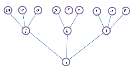
Figure 2. Configurations on semi-finite Cayley tree of order three with levels 2. Schematic diagram to be illustrated the summation used in Equation (3).

For the sake simplicity, denote $Z_{(n+1)}\left(\begin{array}[]{ccc}l&k&j\\ &i&\end{array}\right)=Z_{(n+1)}\left(i;l,k,j\right)$. We have

$$Z_{n+1}\left(i;l,k,j\right) = \sum_{m,w,o,p,r,s,t,u,v\in\{-1,+1\}}[\exp(A(m,w,o,p,r,s,t,u,v))$$

$$Z_{n}\left(l;m,w,o\right)Z_{n}\left(k;p,r,s\right)Z_{n}\left(j;t,u,v\right)],$$

where

$$A(m,w,o,p,r,s,t,u,v) = Ji(j+k+l)+J_{p}i(m+w+o+p+r+s+t+u+v)$$

$$+J_{t}(i(l(m+w+o)+k(p+r+s)+j(t+u+v)),$$

$i,j,k,l\in\{-1,+1\}$ and $n=1,2,\ldots$ (see Figure 2). Therefore, we can calculate the partial partition functions as follows

$$\left\{\begin{array}[]{l}z_{1}^{(n+1)}=a^{3}(bc)^{-9}\left((bc)^{6}z_{1}^{(n)}+3(bc)^{4}z_{2}^{(n)}+3(bc)^{2}z_{3}^{(n)}+z_{4}^{(n)}\right){}^{3}\\ z_{2}^{(n+1)}=a(bc)^{-9}\left((bc)^{6}z_{1}^{(n)}+3(bc)^{4}z_{2}^{(n)}+3(bc)^{2}z_{3}^{(n)}+z_{4}^{(n)}\right){}^{2}\\ \ \ \ \ \ \ \ \ \ \text{}\times\left(b^{6}z_{5}^{(n)}+3c^{2}b^{4}z_{6}^{(n)}+3b^{2}c^{4}z_{7}^{(n)}+c^{6}z_{8}^{(n)}\right)\\ z_{3}^{(n+1)}=a^{-1}(bc)^{-9}\left((bc)^{6}z_{1}^{(n)}+3(bc)^{4}z_{2}^{(n)}+3(bc)^{2}z_{3}^{(n)}+z_{4}^{(n)}\right)\\ \ \ \ \ \ \ \ \ \ \text{}\times\left(b^{6}z_{5}^{(n)}+3c^{2}b^{4}z_{6}^{(n)}+3b^{2}c^{4}z_{7}^{(n)}+c^{6}z_{8}^{(n)}\right){}^{2}\\ z_{4}^{(n+1)}=a^{-3}(bc)^{-9}\left(b^{6}z_{5}^{(n)}+3c^{2}b^{4}z_{6}^{(n)}+3b^{2}c^{4}z_{7}^{(n)}+c^{6}z_{8}^{(n)}\right){}^{3}\end{array}\right.$$

$$\left\{\begin{array}[]{l}z_{5}^{(n+1)}=a^{-3}(bc)^{-9}\left(z_{1}^{(n)}+3(bc)^{2}z_{2}^{(n)}+3(bc)^{4}z_{3}^{(n)}+(bc)^{6}z_{4}^{(n)}\right)^{3}\\ z_{6}^{(n+1)}=a^{-1}(bc)^{-9}\left(z_{1}^{(n)}+3(bc)^{2}z_{2}^{(n)}+3(bc)^{4}z_{3}^{(n)}+(bc)^{6}z_{4}^{(n)}\right)^{2}\\ \ \ \ \ \ \ \ \ \ \text{}\times\left(c^{6}z_{5}^{(n)}+3c^{4}b^{2}z_{6}^{(n)}+3c^{2}b^{4}z_{7}^{(n)}+b^{6}z_{8}^{(n)}\right)\\ z_{7}^{(n+1)}=a(bc)^{-9}\left(z_{1}^{(n)}+3(bc)^{2}z_{2}^{(n)}+3(bc)^{4}z_{3}^{(n)}+(bc)^{6}z_{4}^{(n)}\right)\\ \ \ \ \ \ \ \ \ \ \text{}\times\left(c^{6}z_{5}^{(n)}+3c^{4}b^{2}z_{6}^{(n)}+3c^{2}b^{4}z_{7}^{(n)}+b^{6}z_{8}^{(n)}\right)^{2}\\ z_{8}^{(n+1)}=a^{3}(bc)^{-9}\left(c^{6}z_{5}^{(n)}+3c^{4}b^{2}z_{6}^{(n)}+3c^{2}b^{4}z_{7}^{(n)}+b^{6}z_{8}^{(n)}\right)^{3},\end{array}\right.$$

where $a=e^{\beta J}$, $b=e^{\beta J_{p}}$, $c=e^{\beta J_{t}}$. Noting that

$$\left(z_{2}^{(n+1)}\right)^{3}=\left(z_{1}^{(n+1)}\right)^{2}z_{4}^{(n+1)},\ \left(z_{3}^{(n+1)}\right)^{3}=z_{1}^{(n+1)}\left(z_{4}^{(n+1)}\right)^{2},$$

$$\left(z_{6}^{(n+1)}\right)^{3}=\left(z_{5}^{(n+1)}\right)^{2}z_{8}^{(n+1)},\ \left(z_{7}^{(n+1)}\right)^{3}=z_{5}^{(n+1)}\left(z_{8}^{(n+1)}\right)^{2},$$

only four independent variables remain, and through the introduction of the new variables $u_{i}^{(n+1)}=(z_{2}^{(n+1)})^{\frac{1}{3}}$, we can obtain the recurrence system the following simpler form:

(3.16) $$\left\{\begin{array}[]{l}u_{1}^{(n+1)}=\frac{a}{(bc)^{3}}\left((bc)^{2}u_{1}^{(n)}+u_{4}^{(n)}\right)^{3}\\ u_{4}^{(n+1)}=\frac{1}{a(bc)^{3}}\left(b^{2}u_{5}^{(n)}+c^{2}u_{8}^{(n)}\right)^{3}\\ u_{5}^{(n+1)}=\frac{1}{a(bc)^{3}}\left(u_{1}^{(n)}+(bc)^{2}u_{4}^{(n)}\right)^{3}\\ u_{8}^{(n+1)}=\frac{a}{(bc)^{3}}\left(c^{2}u_{5}^{(n)}+b^{2}u_{8}^{(n)}\right)^{3}.\end{array}\right.$$

Let us define operator as

$$F:u^{(n)}=(u_{1}^{(n)},u_{4}^{(n)},u_{5}^{(n)},u_{8}^{(n)})\in\mathbb{R}^{4}_{+}\rightarrow F(u^{(n)})=(u_{1}^{(n+1)},u_{4}^{(n+1)},u_{5}^{(n+1)},u_{8}^{(n+1)})\in\mathbb{R}^{4}_{+}.$$

Then we can write the recurrence equations (3.16) as $u^{(n+1)}=F(u^{(n)}),n>0$ which in the theory of dynamical systems is called a trajectory of the initial point $u^{(0)}$ under the action of the operator $F$. Thus we can determine the asymptotic behavior of $Z_{n}$ for $n\rightarrow\infty$ by the values of $\lim_{n\rightarrow\infty}u^{(n)}$ i.e., the trajectory of $u^{(0)}$ under the action of the operator $F$. In this paper we study the trajectory (dynamical system) for a given initial point $u^{(0)}\in\mathbb{R}^{4}_{+}$.

4. Dynamics of the operator $F$

4.1. Fixed Points of the operator $F$

In this subsection we are going to determine the fixed points, i.e., solutions to $F(u)=u$. Denote $Fix(F)=\{u:F(u)=u\}.$
We introduce the new variables $\alpha=\sqrt[3]{a}$, $v_{i}=\sqrt[3]{u_{i}}$, for $i=1,4,5,8$. Then the equation $F(v)=v$ becomes

(4.5) $$\left\{\begin{array}[]{l}v_{1}=\frac{\alpha}{(bc)}\left((bc)^{2}v_{1}^{3}+v_{4}^{3}\right)\\ v_{4}=\frac{1}{\alpha(bc)}\left(b^{2}v_{5}^{3}+c^{2}v_{8}^{3}\right)\\ v_{5}=\frac{1}{\alpha(bc)}\left(v_{1}^{3}+(bc)^{2}v_{4}^{3}\right)\\ v_{8}=\frac{\alpha}{(bc)}\left(c^{2}v_{5}^{3}+b^{2}v_{8}^{3}\right).\end{array}\right.$$

4.2. The fixed points of the operator $F$ for $c=1$

Let us consider the following set:

(4.6) $$A=\{(v_{1},v_{4},v_{5},v_{8})\in\mathbb{R}^{4}_{+}:v_{1}=v_{8},v_{4}=v_{5},c=1\}.$$

Note that the set $A$ is invariant with respect to $F$ i.e., $F(A)\subset A.$

Lemma 4.1.

If a vector $\overrightarrow{u}$ is a fixed point of the operator $F$, then $\overrightarrow{u}\in M_{1}:=\{\overrightarrow{u}=(u_{1},u_{4},u_{5},u_{8})\in\mathbf{R}^{4}_{+}:u_{1}=u_{8},u_{4}=u_{5}\}$ or $\overrightarrow{u}\in M_{2}:=\{\overrightarrow{u}=(u_{1},u_{4},u_{5},u_{8})\in\mathbf{R}^{4}_{+}:\left(\sqrt[3]{u_{4}}+\sqrt[3]{u_{5}}\right)^{2}-\sqrt[3]{u_{4}u_{5}}=\psi\left(\left(\sqrt[3]{u_{1}}+\sqrt[3]{u_{8}}\right){}^{2}-\sqrt[3]{u_{1}u_{8}}\right)\}$, where $\psi(y)=\frac{b^{3}+\alpha y(1-b^{4})}{b^{2}\alpha\left(b\alpha y-1\right)}$.

Proof.

From the system (4.5), we have

(4.7) $$\left(v_{1}-v_{8}\right)\left(b\alpha\left(v_{1}^{2}+v_{1}v_{8}+v_{8}^{2}\right)-1\right)+\alpha b^{-1}\left(v_{4}-v_{5}\right)\left(v_{4}^{2}+v_{4}v_{5}+v_{5}^{2}\right)=0$$

(4.8) $$\left(v_{1}-v_{8}\right)(\alpha b)^{-1}\left(v_{1}^{2}+v_{1}v_{8}+v_{8}^{2}\right)+\left(v_{4}-v_{5}\right)(\alpha b)^{-1}\left(b^{2}v_{4}^{2}+b^{2}v_{4}v_{5}+b^{2}v_{5}^{2}+\alpha[b]\right)=0.$$

From (4.7) and (4.8) one can conclude that if $v_{1}=v_{8}$ (respectively $v_{3}=v_{4}$), then $v_{3}=v_{4}$ (respectively $v_{1}=v_{8}$). Therefore, $v_{3}=v_{4}$ if and only if $v_{3}=v_{4}$.

Now let us assume that $v_{1}\neq v_{8}$ and $v_{3}\neq v_{4}$, then we can reduce the equations (4.7) and (4.8) to the following equation:

$$\frac{\alpha b^{-1}\left(v_{4}^{2}+v_{4}v_{5}+v_{5}^{2}\right)}{\left(b\alpha\left(v_{1}^{2}+v_{1}v_{8}+v_{8}^{2}\right)-1\right)}=\frac{\left(b^{2}v_{4}^{2}+b^{2}v_{4}v_{5}+b^{2}v_{5}^{2}+\alpha b\right)}{\left(v_{1}^{2}+v_{1}v_{8}+v_{8}^{2}\right)}.$$

Therefore, from the last equation we have

(4.9) $$v_{4}^{2}+v_{4}v_{5}+v_{5}^{2}=\frac{b^{3}+\alpha\left(v_{1}^{2}+v_{1}v_{8}+v_{8}^{2}\right)(1-b^{4})}{b^{2}\alpha\left(b\alpha\left(v_{1}^{2}+v_{1}v_{8}+v_{8}^{2}\right)-1\right)}.$$

The equation (4.9) gives $\left(\sqrt[3]{u_{4}}+\sqrt[3]{u_{5}}\right)^{2}-\sqrt[3]{u_{4}u_{5}}=\psi\left(\left(\sqrt[3]{u_{1}}+\sqrt[3]{u_{8}}\right){}^{2}-\sqrt[3]{u_{1}u_{8}}\right)$ (see [4]). ∎

Remark 4.1.

The fixed points of the operator $F$ belonging to the set $M_{2}$ give the ferromagnetic phases corresponding to the Ising model (2.1). In order to examine the fixed points of the operator $F$ belonging to the set $M_{2}$ is analytically very difficult. The ferromagnetic phase regions corresponding to the Ising model (2.1) can numerically be determined.

4.3. The existence of paramagnetic and ferromagnetic phases

Let us first study the fixed points of the operator $F$ which belong in $A$ given in the equation (4.6). The fixed points of the operator $F$ determine the paramagnetic phases corresponding to the Ising model (2.1).

The condition $u_{1}=u_{8},u_{4}=u_{5}$ reduces the equation $F(u)=u$ to the following equation

(4.10) $$x=g(x):=\alpha^{2}\left(\frac{1+b^{2}x^{3}}{b^{2}+x^{3}}\right),$$

where $x=\frac{v_{1}}{v_{4}}.$

The following Proposition gives full description of positive fixed points of the function g in (4.10).

Proposition 4.2.

The equation (4.10) (with $x\geq 0,\alpha>0,b>0$) has one solution if $b<1$. Assume that If $b>\sqrt{2}$, then the equation (4.10) has 2 solutions if either $\eta_{1}(b)=\alpha^{-2}$ or $\eta_{2}(b)=\alpha^{-2}$. If $\eta_{1}(b)<\alpha^{-2}<\eta_{2}(b)$ and then there exists $\eta_{1}(b)$, $\eta_{2}(b)$ with $0<\eta_{1}(b)<\eta_{2}(b)$ such that the equation (4.10) has 3 solutions. In this case, we have

$$\eta_{i}(b) = \frac{1}{x_{i}}\left(\frac{1+b^{2}x_{i}^{3}}{b^{2}+x_{i}^{3}}\right),$$

where $x_{i}$ are the solutions of the equation $b^{2}x^{6}-2\left(b^{4}-2\right)x^{3}+b^{2}=0.$.

Proof.

Let us take the first and the second derivatives of the function $g$, we have

(4.11) $$g^{\prime}(x)=\frac{3\left(b^{4}-1\right)x^{2}\alpha^{2}}{\left(b^{2}+x^{3}\right)^{2}},$$

$$g^{\prime\prime}(x)=\frac{6\alpha^{2}\left(b^{4}-1\right)x\left(b^{2}-2x^{3}\right)}{\left(b^{2}+x^{3}\right)^{3}}.$$

From (4.11), if $b<1$ (with $x\geq 0$) then $g$ is decreasing and there can only be one solution of $g(x)=x.$ Thus, we can restrict ourselves to the case in which $b>1.$ It is obvious that the graph of $y=g(x)$ over interval $(0,\sqrt[3]{\frac{b^{2}}{2}})$ is concave up and the graph of $y=g(x)$ over interval $(\sqrt[3]{\frac{b^{2}}{2}},\infty)$ is concave down. As a result, there are at most 3 positive solutions for $g(x)=x.$

According to Preston [15, Proposition 10.7], there can be more than one fixed point of the function $g$ if and only if there is more than one solution to $xg^{\prime}(x)=g(x)$, which is the same as

$$b^{2}x^{6}-2\left(b^{4}-2\right)x^{3}+b^{2}=0.$$

These roots are

$$x_{1}=\sqrt[3]{\frac{-2+b^{4}-\sqrt{4-5b^{4}+b^{8}}}{b^{2}}},x_{2}=\sqrt[3]{\frac{-2+b^{4}+\sqrt{4-5b^{4}+b^{8}}}{b^{2}}}.$$

Note that if $4-5b^{4}+b^{8}\geq 0$, then the roots $x_{1}$ and $x_{2}$ are real numbers. In this case, $4-5b^{4}+b^{8}\geq 0$ if and only if $b\in(0,1)\cap(\sqrt{2},\infty)$. ∎

4.3.1. An Illustrative example for $c=1$.

We have $P_{4}(x)=0$ with a polynomial

(4.12) $$P_{4}=x^{4}-\alpha^{2}b^{2}x^{3}+b^{2}x-\alpha^{2}$$

the coefficients of which depend on parameters $\alpha,b$. Thus we obtain a quartic equation. Such equations can be solved using known formulas (see [20]), since we will have some complicated formulas for the coefficients and the solutions, we do not present the solution here. Nonetheless, we have manipulated the polynomial equation via Mathematica [20]. Here we will only deal with positive fixed points, because of the positivity of exponential functions. We have obtained at most 3 positive real roots for some parameters $J$, $J_{p}$ and $J_{t}=0$ (coupling constants) and temperature $T$.

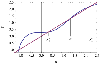
Figure 3. (Color online) There exist three positive roots of the equation (4.10) for $J=-4.5,J_{p}=14,T=24.6$.

For example, Fig. 3 shows that there are 3 positive fixed points of the function (4.10) for $J=-4.5,J_{p}=14,J_{t}=0,T=24.6$. These all fixed points are $x_{0}^{*}=-1.02554,x_{1}^{*}=0.306205,x_{2}^{*}=1.28008,x_{3}^{*}=2.20209$, respectively. It is clear that $x_{1}^{*}=0.306205,x_{3}^{*}=2.20209$ are stable, and $x_{2}^{*}=1.28008$ is unstable. The point $x_{cr}=1.15992$ is the breaking point of the function $g$. There are two extreme paramagnetic phases associated to the positive fixed points.

4.4. Periodic Points of the operator $F$

One of the most interested problems in the investigation of non linear dynamical systems is the existence of periodic points. While, for the one-dimensional case, every non linear dynamical systems contains periodic points there is a $d$-dimensional ($d>1$) which contains no periodic points. In statistical physics, these periodic points reveal the phase types corresponding to the given model. We recall some definitions and results first.

Definition 4.3.

A point $\textbf{u}=(u_{1},u_{4},u_{5},u_{8})$ in $\mathbf{R}^{4}_{+}$ is called a periodic point of $F$ if there exists $p$ so that $F^{p}(\textbf{u})=\textbf{u}$ where $F^{p}$ is the $p$th iterate of $F$. The smallest positive integer $p$ satisfying the above is called the prime period or least period of the point u. Denote by Per${}_{p}(F)$ the set of periodic points with prime period $p$.

Let us first describe periodic points with $p=2$ on $M_{1}$ in this case the equation $F(F(\textbf{u}))=\textbf{u}$ can be reduced to a description of 2-periodic points of the function $g$ defined in (4.10) i.e., to a solution of the equation

(4.13) $$g(g(x))=x.$$

Note that the fixed points of f are solutions to (4.13), to find other solutions we consider the equation

$$\frac{g(g(x))-x}{g(x)-x}=0,$$

simple calculations show that the last equation is equivalent to the following

(4.14) $$p_{6}(x):=4b^{2}(1+b^{4}\alpha^{6})x^{6}+\alpha^{2}(b^{4}-1)x^{5}+b^{2}\alpha^{4}(b^{4}-1)x^{4}+2b^{4}(1+\alpha^{6})x^{3}$$

$$+b^{2}\alpha^{2}(b^{4}-1)x^{2}+\alpha^{4}(b^{4}-1)x+b^{2}(b^{4}+\alpha^{6})=0.$$

In order to describe the periodic points with $p=2$ on $M_{1}$ of the operator $F$, we should find the solutions to (4.14) which are different from the solutions of the equation (4.12). On the other words, we obtain the set

(4.15) $$M_{3}:=\{(u_{1},u_{4},u_{5},u_{8})\in\mathbf{R}^{4}_{+}:g(g(x))=x\}.$$

Therefore, we should examine the roots of the polynomial $p_{6}(x)$ of degree 6. As mentioned above, the roots of such polynomials can be described using known formulas. Since some complicated formulas for the coefficients and the solutions are included, we will not present the solution here. In order to illustrate the problem, we have manipulated the equation (4.13) via Mathematica [20] (see Figure 4 (red color)). The black graph in the Figure 4 represents the roots of the nonlinear function $y=g(x).$

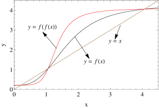
Figure 4. (Color online) There exist three positive roots of the equation (4.13) (black color) for $J=-6,J_{p}=56.9,T=75$. Also, the equation (4.13) has three positive roots (red color) for $J=-6,J_{p}=56.9,T=75$.

We can obtain an initial point of the sequence $(u_{1}^{(n)},u_{4}^{(n)},u_{5}^{(n)},u_{8}^{(n)})$ under positive boundary condition as follows:

$$\textbf{u}_{0}=(u_{1}^{(0)},u_{4}^{(0)},u_{5}^{(0)},u_{8}^{(0)})=(ab^{3}c^{3},\frac{b^{3}}{ac^{3}},\frac{1}{ac^{3}b^{3}},\frac{ac^{3}}{b^{3}}).$$

In order to study some useful features of the function $g$, let us give the following lemma.

Lemma 4.4.

1) If $b>1$ then the sequence $x_{n}=(x_{n-1})$, $n=1,2,...$ converges for the initial point $x_{0}=\sqrt[3]{\frac{u_{1}^{(0)}}{u_{4}^{(0)}}}=\alpha^{2}>0$ under positive boundary condition, where $g$ is defined in (4.10).

2) If $b<1$ then the sequence $y_{n}=f(y_{n-1})$, $n=1,2,...$ converges for the initial point $y_{0}=\frac{\alpha^{2}\left(1+b^{2}\alpha^{6}\right)}{b^{2}+\alpha^{6}}>0$ under positive boundary condition, where $f(x)=g(g(x)).$

Proof.

1) For $b>1$ we have $g^{\prime}(x)=\frac{3\left(b^{4}-1\right)x^{2}\alpha^{2}}{\left(b^{2}+x^{3}\right)^{2}}>0$ i.e., $g$ is an increasing function. Here we consider the case when the function $g$ has three fixed points $x^{*}_{i},i=1,2,3$ (see Proposition 4.2 and Figure 3). We have that the point $x^{*}_{2}$ is a repeller i.e., $g^{\prime}(x^{*}_{2})>1$ and the points $x^{*}_{1},x^{*}_{3}$ are attractive i.e., $g^{\prime}(x^{*}_{1})<1$ and $g^{\prime}(x^{*}_{3})<1$. Now we shall take arbitrary $x_{0}>0$ and prove that $x_{n}=g(x_{n-1})$, $n\geq 1$ converges as $n\rightarrow\infty$. For any $x\in(0,x^{*}_{1})$ we have $x<g(x)<x^{*}_{1}$, since $g$ is an increasing function, from the last inequalities we get $x<g(x)<g^{2}(x)<g(x^{*}_{1})=x^{*}_{1}$. Iterating this argument we obtain $g^{n-1}(x)<g^{n}(x)<x^{*}_{1}$, which for any $x_{0}\in(0,x^{*}_{1})$ gives $x_{n-1}<x_{n}<x^{*}_{1}$ i.e., $x_{n}$ converges and its limit is a fixed point of $g$, since $g$ has a unique fixed point $x^{*}_{1}$ in $(0,x^{*}_{1}]$. We conclude that the limit is $x^{*}_{1}$. For $x\in(x^{*}_{1},x^{*}_{2})$ we have $x^{*}_{2}>x>g(x)>x^{*}_{1}$, consequently $x_{n}>x_{n+1}$ i.e., $x_{n}$ converges and its limit is again $x^{*}_{1}$. Similarly, one can show that if $x_{0}>x^{*}_{2}$ then $x_{n}\rightarrow x^{*}_{3}$ as $n\rightarrow\infty$.

2) For $b<1$ we have $g$ is decreasing and has a unique fixed point $x_{1}$ which is repelling, but $f$ is increasing since $f^{\prime}(x)=g^{\prime}(g(x))g^{\prime}(x)>0$. We have that $f$ has at most three fixed points (including $x_{1}$). The point $x_{1}$ is repelling for $f$ too, since $f^{\prime}(x_{1})=g^{\prime}(g(x_{1}))g^{\prime}(x_{1})=(g^{\prime}(x_{1}))^{2}>1$. But fixed points $x_{-},x_{+}$ of $f$ are attractive. Hence one can repeat the same argument of the proof of the part 1) for the increasing function $f$ and complete the proof. ∎

4.5. The phase diagrams of the model

For plotting of the phase diagrams in the Hamiltonian three-parameter spaces, the following choice of reduced variables is convenient:

(4.16) $$x^{(n)}=\frac{u_{4}^{(n)}+u_{5}^{(n)}}{u_{1}^{(n)}+u_{8}^{(n)}},\ y^{(n)}=\frac{u_{1}^{(n)}-u_{8}^{(n)}}{u_{1}^{(n)}+u_{8}^{(n)}},\ z^{(n)}=\frac{u_{4}^{(n)}-u_{5}^{(n)}}{u_{1}^{(n)}+u_{8}^{(n)}}.$$

The variable $x^{(n)}$ is just a measure of the frustration of the nearest-neighbor bonds and is not an order parameter like $y^{(n)},z^{(n)}$. It is convenient to know the broad features of the phase diagram before discussing the different transitions in more detail (see [14] for details). This can be achieved numerically in a straightforward fashion.

Let $T/J=\alpha$, $-J_{p}/J=\beta$, $-J_{t}/J=\gamma$ and respectively $a=\exp(\alpha^{-1}),b=\exp(-\alpha^{-1}\beta)$ and $c=\exp(-\alpha^{-1}\gamma)$. From the equations (4.16), we can obtain the following recurrence dynamical system:

(4.22) $$\left\{\begin{array}[]{l}x^{(n+1)}=\frac{\left(c^{2}\left(1-y^{(n)}\right)+b^{2}\left(x^{(n)}-z^{(n)}\right)\right)^{3}+\left(1+y^{(n)}+b^{2}c^{2}\left(x^{(n)}+z^{(n)}\right)\right)^{3}}{a^{2}\left(\left(x^{(n)}+b^{2}c^{2}\left(1+y^{(n)}\right)+z^{(n)}\right)^{3}+\left(b^{2}\left(1-y^{(n)}\right)+c^{2}\left(x^{(n)}-z^{(n)}\right)\right)^{3}\right)}\\ \\ y^{(n+1)}=\frac{\left(x^{(n)}+b^{2}c^{2}\left(1+y^{(n)}\right)+z^{(n)}\right)^{3}-\left(b^{2}\left(1-y^{(n)}\right)+c^{2}\left(x^{(n)}-z^{(n)}\right)\right)^{3}}{\left(x^{(n)}+b^{2}c^{2}\left(1+y^{(n)}\right)+z^{(n)}\right)^{3}+\left(b^{2}\left(1-y^{(n)}\right)+c^{2}\left(x^{(n)}-z^{(n)}\right)\right)^{3}}\\ \\ z^{(n+1)}=\frac{\left(c^{2}\left(1-y^{n}\right)+b^{2}\left(x^{n}-z^{n}\right)\right)^{3}-\left(1+y^{n}+b^{2}c^{2}\left(x^{n}+z^{n}\right)\right)^{3}}{a^{2}\left(\left(x^{n}+b^{2}c^{2}\left(1+y^{n}\right)+z^{n}\right)^{3}+\left(b^{2}\left(1-y^{n}\right)+c^{2}\left(x^{n}-z^{n}\right)\right)^{3}\right)}.\end{array}\right.$$

The system of three equations finally obtained in (4.22) is less complicated than one might have anticipated. It remains difficult to tackle analytically apart from simple limits and numerical methods are necessary to study its detailed behavior (see [14]).

Starting from initial conditions

(4.26) $$\left\{\begin{array}[]{l}x^{(1)}=\frac{1}{a^{2}c^{6}},\\ y^{(1)}=\frac{b^{6}-1}{b^{6}+1},\\ z^{(1)}=\frac{b^{6}-1}{a^{2}c^{6}(b^{6}+1)}.\end{array}\right.$$

that corresponds to positive boundary condition $\bar{\sigma}^{(n)}(V\setminus V_{n})\equiv 1,$ one iterates the recurrence relations (3.16) and observes behavior of the phase diagrams after a large number of iterations ($n=10000$). For the fixed points, the corresponding magnetization $m$ is given by

(4.27) $$m^{(n)}=\frac{\left(1+x^{(n)}+y^{(n)}+z^{(n)}\right)^{3}-\left(1+x^{(n)}-y^{(n)}-z^{(n)}\right)^{3}}{\left(1+x^{(n)}+y^{(n)}+z^{(n)}\right)^{3}+\left(1+x^{(n)}-y^{(n)}-z^{(n)}\right)^{3}}.$$

The initial point of the magnetization $m$ can be obtained as;

(4.28) $$m^{(1)}=\frac{(b^{2}-1)\left((1+b^{2})^{2}-b^{2}\right)\left((1+b^{6})^{2}-b^{6}\right)}{\left(1+b^{2}\right)\left(1-b^{2}+b^{4}\right)\left(1-b^{6}+b^{12}\right)}.$$

Here the variable $x$ is a measure of the frustration of the nearest-neighbor bonds [14]. Since for a paramagnetic phase we have $u_{1}=u_{8}$ and $u_{4}=u_{5}$, we get $y^{(n)}=z^{(n)}\rightarrow 0$. Hence $m=0$, but in case of coexistence of several paramagnetic phases their measure of the frustration (i.e. $x$) are different. These different values of $x$ are the solutions to (4.10).

Now, assume that $c=\exp(-\alpha^{-1}\gamma)=1$. In the simplest situation a fixed point $\textbf{u}^{*}=(u^{*}_{1},u^{*}_{4},u^{*}_{5},u^{*}_{8})\in\mathbf{R}^{4}_{+}$ is reached. Possible initial conditions with respect to different boundary conditions can be obtained in [14, 36]. In this paper, we consider initial conditions (4.26) and (4.28). Depending on $u^{*}_{1},u^{*}_{4},u^{*}_{5},u^{*}_{8}$, in the simplest situation a fixed point $(x^{*},y^{*},z^{*})$ is reached. It corresponds to a paramagnetic phase (briefly P) if $y^{*}=0,z^{*}=0$ or to a ferromagnetic phase (briefly F) if $y^{*},z^{*}\neq 0.$ The system may be periodic with period $p$, i.e. the periodic phase is a configuration with some period. If the case $p=2$ corresponds to antiferromagnetic phase (briefly P2) and the case $p=4$ corresponds to so-called antiphase (briefly P4), that denoted  $<2>$ for compactness in [14, 36].

Finally, the system may remain aperiodic, i.e. very long period to compute or non-periodic. The distinction between a truly aperiodic case and one with a very long period is difficult to make numerically. Detailed information about the phase analysis and the relation with partition functions, it is mainly refered to works given by Vannimenus [14], Uguz et al [35] and Mariz et al [36]. Below we just consider periodic phases with period $p$ where $p\leq 12$ (briefly P2-P12).

It corresponds to (see [14, 36, 37] for details) the cases in Lemma 4.1:

• a paramagnetic phase: if $\textbf{u}^{*}\in M_{1}$, in the figure 5 (b), the white regions represent the paramagnetic phase. This represents the set $M_{1}$ given in Lemma 4.1;

• a ferromagnetic phase: if $\textbf{u}^{*}\in M_{2}$, in the figure 5 (b), the red regions represent the ferromagnetic phase. This represents the set $M_{2}$ given in Lemma 4.1;

• in the figure 5 (b), the yellow regions represent the P2 phase. This represents the set $M_{3}$ given in (4.15).

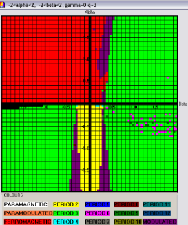
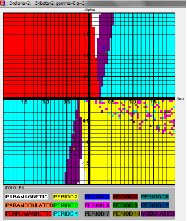
Figure 5. (Color online) (a) Phase diagram of the model for $J_{p}=0$; (b) Phase diagram of the model for $J_{t}=0$.

Figure 5 (a) and (b) show the phase diagrams of the model on Cayley tree of order three. Contrary to the Vannimenus’s work [14], here the multicritical Libschit points appear in non-zero points. In Figure 5 (a), we observe that the phase diagram contains ferromagnetic (F), period-2, period-3 and modulated phases. In Figure 5 (b), the phase diagram consists of ferromagnetic (F), paramagnetic (P) (fixed point), chaotic (C) (or modulated), and antiferromagnetic + + - - (four cycle antiferromagnetic phase) phases. In the chaotic phase, small regions with periodic orbits corresponding to commensurate phases are observed. Although it is difficult, to distinguish long period behavior from chaos, it seems that the behavior in the intermediate region is predominantly chaotic [36]. Note that the modulated phase can consist of commensurate (periodic) and incommensurate (aperiodic) regions corresponding to the so called ”devil s staircase”. In order to distinguish these phases from each other, one needs to analysis the modulated phase regions via Lyapunov exponent and the attractors in detail (see [35, 36, 37, 38]). Here, we will not give these details.

From Proposition 4.2, we have the following theorem

Theorem 4.5.

The model (2.1) (with $x\geq 0,\alpha>0,b>0$) has a unique paramagnetic phase if $b<1$. Assume that If $b>\sqrt{2}$, then the model (2.1) has exactly two paramagnetic phases if either $\eta_{1}(b)=\alpha^{-2}$ or $\eta_{2}(b)=\alpha^{-2}$. If $\eta_{1}(b)<\alpha^{-2}<\eta_{2}(b)$ and then there exists $\eta_{1}(b)$, $\eta_{2}(b)$ with $0<\eta_{1}(b)<\eta_{2}(b)$ such that the model (2.1) has exactly three paramagnetic phases.

4.6. The fixed points of the operator $F$ for $b=1$

In the equation (4.5), if we assume as $b=1$, then we have

(4.33) $$\left\{\begin{array}[]{l}v_{1}=\frac{\alpha}{c}\left(c^{2}v_{1}^{3}+v_{4}^{3}\right)\\ v_{4}=\frac{1}{\alpha c}\left(v_{5}^{3}+c^{2}v_{8}^{3}\right)\\ v_{5}=\frac{1}{\alpha c}\left(v_{1}^{3}+c^{2}v_{4}^{3}\right)\\ v_{8}=\frac{\alpha}{c}\left(c^{2}v_{5}^{3}+v_{8}^{3}\right).\end{array}\right.$$

Now, we describe the positive fixed points of system (4.33). Let us consider the following set

(4.34) $$B:=\{(v_{1},v_{4},v_{5},v_{8})\in\mathbf{R}^{4}_{+}:v_{1}=v_{8},v_{4}=v_{5}\}.$$

Remark 4.2.

From the system (4.33), it is clear that the equations $v_{1}=v_{8}$ and $v_{4}=v_{5}$ don’t satisfy, i.e., the set $B$ given in (4.34) is empty. Therefore, the paramagnetic phase regions in the phase diagrams associated with the model disappear in $[-2,2]\times[-2,2]\subset\mathbf{R}^{2}$.

In [18], we studied the phase diagram and extreme Gibbs measures of the Ising model on a two order Cayley tree in the presence of competing binary and ternary interactions, we have observed that the P regions completely disappears in the phase diagram associated with the model (2.1) for $b=1$.

5. Conclusions

Written for both mathematics and physics audience, this paper has a fourfold purpose: (1) to study analytically the recurrence equations associated with the model (2.1); (2) to obtain numerically the paramagnetic, the ferromagnetic and period 2 regions corresponding to the sets $M_{1},M_{2},B$, respectively; (3) to illustrate the fixed points of corresponding operator; (4) to compare the numerical results to exact solutions of the model.

We state some unsolved problems that turned out to be rather complicated and require further consideration:

1. Do any other invariant sets of the operator $F$ exist?

2. Do positive fixed points of the operator $F$ exist outside the invariant sets?

3. Does there exist a periodic points ($p>2$) of rather cumbersome high-order equations that can be solved by analytic methods?

In the first case we have already obtained the fixed points of the operator $F$ such that $u_{1}=u_{8}$ and $u_{4}=u_{5}$. For the periodic case, however, it is not possible to obtain all solutions satisfying all requirements of Equations (3.16) such that $\{\textbf{u}=(u_{1},u_{4},u_{5},u_{8})\in\mathbf{R}^{4}_{+}:F^{p}(\textbf{u})=\textbf{u},p>1\}$ is invariant. The proof of this statement is involved with a number mathematical complexity. Also, in the second case ($b=1$), to find analytically the fixed points of the operator $F$ is much more difficult.

By using the standard approach, we have proved the existence of phase transition for paramagnetic phase when $J_{p}>0$ and for phase with period 2 when $J_{p}<0$. These results fully consistent with numerical results in [14]. In [3], the authors have analytically studied the recurrence equations and obtain some exact results: critical temperatures and curves, number of phases, partition function for the Ising model on a second-order Cayley tree. The problem can numerically be examined by the approach in [14]. In the present paper, we analytically investigate the fixed points of the dynamical system associated with the Ising model on a rooted Cayley tree of order three by solving a system of nonlinear functional equations (see [13, 16] for details).

References

• [1] Akın H., Rozikov U. A., and Temir S., A new set of limiting Gibbs measures for the Ising model on a Cayley tree, J. Stat. Phys. 142 (2), 314-321 (2011). doi: 10.1007/s10955-010-0106-6
• [2] Ganikhodjaev N. N., Akın H., Uguz S., Temir S., Phase diagrams of an Ising system with competing binary, prolonged ternary and next-nearest interactions on a Cayley tree, J. Concrete and Applicable Mathematics, 9 (1), (2011), 26-34.
• [3] Rozikov U. A., Akın H., and Uguz S., Exact Solution of a generalized ANNNI model on a Cayley tree, Math. Phys. Anal. Geom. 17, 103 -114 (2014). doi: 10.1007/s11040-014-9144-7
• [4] Ganikhodjaev, N. N. and Uguz S., Competing binary and tuple interactions on a Cayley tree of arbitrary order, Physica A, 390, 23-24 (1), 4160-4173 (2011).
• [5] Akın H. and Saygılı H., Phase transition of the Potts model with three competing interactions on Cayley tree of order 3, AIP Conference Proceedings 1676, 020026 (2015). doi: http://dx.doi.org/10.1063/1.4930452
• [6] Akın H., Using New Approaches to obtain Gibbs Measures of Vannimenus model on a Cayley tree, Chinese Journal of Physics, 54 (4), 635-649 (2016). doi: 10.1016/j.cjph.2016.07.010
• [7] Akın H., Phase transition and Gibbs measures of Vannimenus model on semi-infinite Cayley tree of order three, Int. J. Mod. Phys. B, 31 (13), 1750093 (2017) [17 pages] doi: 10.1142/S021797921750093X
• [8] Akın, H. (2017). Gibbs Measures with memory of length 2 on an arbitrary order Cayley tree. arXiv preprint arXiv:1701.00715.
• [9] Bleher P. M., Ruiz J., and Zagrebnov V. A., On the purity of the limiting Gibbs state for the Ising model on the Bethe lattice, J. Stat. Phys., 79, 473-482 (1995). doi: 10.1007/BF02179399
• [10] Lebowitz, J. L., Coexistence of phases in Ising ferromagnets, J. Stat. Phys., 16 (6), 463-476 (1977). doi: 10.1007/BF01152284
• [11] Bleher P. M., and Ganikhodjaev N. N., On pure phases of the Ising model on the Bethe lattices, Theory Probab. Appl. 35, 216-227 (1990). doi: 10.1137/1135031
• [12] Ganikhodjaev N. N., Temir S., and Akın H., Modulated phase of a Potts model with competing binary interactions on a Cayley tree, J. Stat. Phys., 137, 701-715 (2009). doi: 10.1007/s10955-009-9869-z
• [13] Ganikhodjaev N. N., Akın H., and Temir T., Potts model with two competing binary interactions, Turk. J Math., 31 (3), 229-238 (2007).
• [14] Vannimenus J., Modulated phase of an Ising system with competing interactions on a Cayley tree, Zeitschrift fur Physik B Condensed Matter 43 (2), 141-148 (1981). doi: 10.1007/BF01293605
• [15] Preston Ch. J., Gibbs States on Countable Sets, Cambridge Univ.Press, Cambridge (1974).
• [16] Akın H., and Temir S., On phase transitions of the Potts model with three competing interactions on Cayley tree, Condensed Matter Physic. 14 (2), 23003:1-11 (2011). doi: 10.5488/CMP.14.23003
• [17] Ganikhodjaev N. N., Akın H., Uguz S., and Temir T., On extreme Gibbs measures of the Vannimenus model, J. Stat. Mech. Theor. Exp. 03 (2011): P03025. doi: 10.1088/1742-5468/2011/03/P03025
• [18] Ganikhodjaev N. N., Akın H., Uguz S., and Temir S., Phase diagram and extreme Gibbs measures of the Ising model on a Cayley tree in the presence of competing binary and ternary interactions, Phase Transitions 84, no. 11-12, 1045 -1063 (2011). doi: 10.1080/01411594.2011.579395
• [19] Rozikov U. A., Gibbs Measures on Cayley trees, World Scientific Publishing Company (2013).
• [20] Wolfram Research, Inc., Mathematica, Version 8.0, Champaign, IL (2010).
• [21] Ganikhodjaev N. N., and Rozikov U. A., Description of periodic extreme gibbs measures of some lattice models on the Cayley tree, Theor. Math. Phys. 111, 480-486 (1997). doi: 10.1007/BF02634202
• [22] Akın H., Ganikhodjaev, Uguz S., and Temir S., Periodic extreme Gibbs measures with memory length 2 of Vannimenus model, AIP Conf. Proc. 1389 (1), 2004 -2007, (2011). doi: 10.1063/1.3637008.
• [23] Akın H., Uguz S., Temir S., Behaviors of phase diagrams of an Ising model on a Cayley tree-like lattice: Rectangular chandelier, AIP Conf. Proc., 1281, 607-611 (2010). doi: 10.1063/1.3498550.
• [24] Uguz S., and Akın H., Modulated Phase of an Ising System with quinary and binary interactions on a Cayley tree-like lattice: Rectangular Chandelier. Chin. J. Phys. 49 (3), 788-801 (2011).
• [25] Uguz S., and Akın H., Phase diagrams of competing quadruple and binary interactions on Cayley tree-like lattice: Triangular Chandelier, Physica A 389, 1839 (2010). doi: 10.1016/j.physa.2009.12.057
• [26] Moraal H., Ising spin systems on Cayley tree-like lattices: Spontaneous magnetization and correlation functions far from the boundary, Physica A 92, 305-314 (1978). doi: 10.1016/0378-4371(78)90037-7
• [27] Akın H., Ganikhodjaev N. N., Temir S., Uguz S., Description of extreme Gibbs measures for the Ising model with three interactions, Acta Physica Polonica A, 123 (2), 484-487 (2013). doi: 10.12693/APhysPolA.123.484
• [28] Uguz S., Ganikhodjaev N. N., Akın H., Temir S., The competing interactions on a Cayley tree-like lattice: Pentagonal Chandelier, Acta Physica Polonica A, 121 (1), 114-118 (2012). doi: 10.12693/APhysPolA.121.114
• [29] Bleher P., Zalys E., Limit Gibbs distributions for the Ising model on hierarchical lattices, Lithuanian Mathematical Journal, 28 (2), 127-39 (1988).
• [30] Bleher, P.M., Extremity of the disordered phase in the Ising model on the Bethe lattice, Communications in Mathematical Physics, 128 (2), 411-419 (1990). doi: 10.1007/BF02108787
• [31] Akın H., Temir S., Phase transitions for Potts model with four competing interactions, Condensed Matter Physics, 14 (2), 23003: 1-11 (2011). doi: 10.5488/CMP.14.23003
• [32] Mukhamedov F., Akın H. and Khakimov O., Gibbs measures and free energies of Ising-Vannimenus Model on the Cayley tree, J. Stat. Mech. 2017 (053101-059701) 053208 https://doi.org/10.1088/1742-5468/aa6c88
• [33] Nazarov Kh A., and Rozikov U., Periodic Gibbs measures for the Ising model with competing interactions, Theoretical and mathematical physics 135 (3), 881-888 (2003). doi: 10.1023/A:1024091206594
• [34] Kindermann, R. and Snell, J.L.: Markov Random Fields and Their Applications, Contemporary Mathematics. V.1, Providence,Rhode Island: Amer. Math. Soc., 1980.
• [35] Uguz S., Ganikhodjaev N. N., Akın H., Temir S., Lyapunov exponent and modulated phases for the Ising system with competing interactions on a Cayley tree of arbitrary order, Int. Journal of Modern Physics C, 23 (5), (2012), DOI: 10.1142/S0129183112500398
• [36] Mariz M., Tsalis C., Albuquerque A.L., Phase diagram of the Ising model on a Cayley tree in the presence of competing interactions and magnetic field, Jour. Stat. Phys. 40, 577-592 (1985).
• [37] Inawashiro S., Thompson C. J. and Honda G., Ising model with competing interactions on a Cayley tree, J. Stat. Phys. 33, 419-436 (1983).
• [38] Inawashiro S. and Thompson, C.J., Competing Ising interactions and chaotic glass-like behaviour on a Cayley tree, Physics Letters A, 97, 245-248 (1983).