Time Domain Filtering of Resolved Images of Sgr A*

Abstract

The goal of the Event Horizon Telescope (EHT) is to provide spatially resolved images of Sgr A*, the source associated with the Galactic Center black hole. Because Sgr A* varies on timescales short compared to an EHT observing campaign, it is interesting to ask whether variability contains information about the structure and dynamics of the accretion flow. In this paper, we introduce “time-domain filtering”, a technique to filter time fluctuating images with specific temporal frequency ranges, and demonstrate the power and usage of the technique by applying it to mock millimeter wavelength images of Sgr A*. The mock image data is generated from General Relativistic Magnetohydrodynamic (GRMHD) simulation and general relativistic ray-tracing method. We show that the variability on each line of sight is tightly correlated with a typical radius of emission. This is because disk emissivity fluctuates on a timescale of order the local orbital period. Time-domain filtered images therefore reflect the model dependent emission radius distribution, which is not accessible in time-averaged images. We show that, in principle, filtered data have the power to distinguish between models with different black hole spins, different disk viewing angles, and different disk orientations in the sky.

1 Introduction

The Event Horizon Telescope (EHT) is a global very long baseline interferometry (VLBI) network that will soon produce time- and space- resolved images of the hot plasma close to the event horizon of the supermassive black holes at the center of M87 and the Milky Way (Doeleman et al., 2009). Already it is clear that both sources have structure on event horizon scales (Doeleman et al., 2008, 2012), and that in Sgr A* the source varies on short timescales in both total and polarized intensities (Fish et al., 2011; Johnson et al., 2015). When fully deployed, the EHT promises to offer higher sensitivity, greater dynamic range, and greater angular resolution. This may enable EHT to image the “photon ring”, a surface brightness feature that appears on lines of sight passing close to the photon orbit; given the accurately measured ratio of black hole mass to distance (see Psaltis et al., 2015; Johannsen et al., 2016), the angular radius of the photon ring is uniquely predicted by general relativity (Bardeen, 1973; Luminet, 1979).

At the same time, theoretical developments in modeling black hole accretion and interpreting EHT data are progressing at a very rapid pace. In addition to stationary phenomenological models of black hole accretion flows (e.g. Narayan & Yi, 1994; Broderick et al., 2009, 2016), General Relativistic, ideal Magnetohydrodynamics (GRMHD) codes are now widely available to model time-dependent accretion flows and jets (e.g. Gammie et al., 2003; De Villiers et al., 2003; Noble et al., 2009; Mościbrodzka et al., 2014; White et al., 2016). Some models (e.g. Chandra et al., 2015; Ressler et al., 2015; Foucart et al., 2016) go beyond the ideal fluid approximation and account for the collisionless nature of the accreting plasma, including variations in the ratio of ion to electron temperature. Widely available relativistic radiative transfer schemes (e.g. Noble et al., 2007; Dolence et al., 2009; Shcherbakov & McKinney, 2013; Schnittman & Krolik, 2013; Chan et al., 2015b; Dexter, 2016; Narayan et al., 2016; Gold et al., 2017) can, given accurate information about the electron distribution function, now produce mock images, polarization maps, and spectra of model accretion flows.

Still, there are obstacles to realizing the full potential of EHT. Three of the most interesting challenges for Sgr A* are (1) distortion of the images by electron scattering in the interstellar medium; (2) theoretical uncertainties related to the structure and dynamics of the accretion flow; (3) interpreting the time-dependence of the source, since the intrinsic variability timescales are comparable to or smaller than the on-source integration time (Lu et al., 2016; Medeiros et al., 2016, 2017).

A large number of pan-chromatic campaigns including radio, Near-Infrared (NIR), mm/sub-mm, and X-ray have analyzed the Sgr A* light curves in the context of characteristic timescale (e.g. Do et al., 2009; Meyer et al., 2009; Dexter et al., 2014) and flaring emission (e.g. Baganoff et al., 2001; Genzel et al., 2003; Hornstein et al., 2007; Eckart et al., 2008; Marrone et al., 2008; Porquet et al., 2008; Dodds-Eden et al., 2009; Yusef-Zadeh et al., 2009; Trap et al., 2011; Haubois et al., 2012; Neilsen et al., 2013). While those studies have revealed the existence of a complex time-variable emission mechanism likely caused by a magnetized turbulent accretion flow (e.g. Bower et al., 2005), a plausible interpretation can be obtained only through the time- and space- resolved EHT observations. Previous VLBI observations have shown evidence of structural (Fish et al., 2016) and magnetic field configuration (Johnson et al., 2015) variabilities with a limited number of baselines. Forthcoming EHT will provide far more information on the spatial structure of Sgr A*.

It is important to prepare a set of tools to extract information of the underlying dynamics from the time variability since intrinsic variability in EHT observations of Sgr A* is likely. Here, we introduce a “time-domain filtering” technique that produces images of the temporal power in an arbitrary frequency range. The technique is in principle applicable to any kind of time fluctuating images, and this paper is aimed at demonstration of the usage and power of the technique by applying it to mock EHT observations. We explore what information might be extracted from that variability using our technique. Does variability convey information about turbulence in the accretion flow? Can this information be extracted from even ideal mock data? We do not attempt to generate realistic simulated data that includes the effects of instrumental and atmospheric noise, weather, Earth rotation, and interstellar scattering. Instead we consider time-dependent, “bare” mock images of the simulations. We ask (1) how is the frequency of observational image fluctuations linked to conditions in the emission region in the disk? (2) does time-domain filtering of the images permit one to distinguish between different models?

The plan of the paper is as follows. §2 describes time-dependent dynamical and radiative models of the accretion flow. §3 presents method and results of the image filtering. §4 discusses the link between the image variability and the emission region in the disk, and §5 summarizes the results.

2 Simulation

To investigate the effects of time-domain filtering, we run an ideal GRMHD simulation of a black hole accretion flow with a small mean magnetic field. The flow is assumed radiatively inefficient, so cooling is negligible. This is well justified for Sgr A* Dibi et al. (2012). We then estimate the emergent radiation using a relativistic radiative transport code.

2.1 Accretion Disk Simulation

We evolve the accretion flow using the conservative GRMHD code harm3d (Noble et al., 2006, 2009). The simulation starts from a constant angular momentum equilibrium torus Fishbone & Moncrief (1976) that is perturbed by a weak magnetic field to seed the growth of the Magnetorotational Instability (MRI). The disk is integrated in Kerr-Schild spacetime in modified spherical-polar coordinates, with a logarithmically scaled radial grid. The computational domain runs from within the event horizon to 240$GM_{\rm{BH}}/c^{2}$ in radius and extends over a full $2\pi$ radians in azimuth. The radial and poloidal boundary condition are set to outflow and reflective boundary, respectively. The simulation is terminated after 14000$GM_{\rm{BH}}/c^{3}$, which is long compared to the timescale for the MRI to reach saturation but short compared to the accretion timescale for the torus. Our initial conditions have only a small net vertical magnetic flux through the disk, and so produce a Standard and Normal Evolution (SANE, Narayan et al. 2012) disk model with short timescale variability that is qualitatively consistent with observational results (Chan et al., 2015a).

We run 2 models with different black hole spin: a rapidly spinning black hole with $a=0.9375$ (hereafter $0.94$) with resolution $260{\times}192{\times}128$ (in radius, colatitude, and longitude respectively), and a nonrotating black hole ($a=0$) with resolution $144{\times}144{\times}144$. The difference in resolution arises because of computational limitations. One might worry that the difference would produce differences in time variability properties, but this appears not to be the case; as one indication, the azimuthal correlation length of the emissivity, which is tightly correlated to the observational variability as will be discussed in §4, differs by only 10% on average at $r<12GM_{\rm{BH}}/c^{2}$ (azimuthal correlation length of fluid variables is discussed in Shiokawa et al. 2012), while the Innermost Stable Circular Orbit (ISCO) orbital frequency differs by a factor of $\sim 4$; 34 minutes and 9 minutes for $a=$0 ($R_{\rm{ISCO}}=6GM_{\rm{BH}}/c^{2}$) and 0.94 ($R_{ISCO}\sim 2.04GM_{\rm{BH}}/c^{2}$), respectively. This suggests that the artificial error introduced by the resolution difference has only a minor effect on the observational variability in our radiative models.

Hereafter, we describe both the length unit $GM_{\rm{BH}}/c^{2}\sim 6.64{\times}10^{11}$ cm and time unit $GM_{\rm{BH}}/c^{3}\sim 22$ seconds as $M$ by setting $GM_{\rm{BH}}=c=1$ unless otherwise indicated.

2.2 Radiative Model

The next step is to construct time-variable images of the model. The total duration of our model is $2500M$ ($\sim 15$ hrs for Sgr A*) taken from the last part of our accretion disk simulation. We use the ray-tracing method of Noble et al. (2007, 2009) that integrates the transfer equation along null geodesics, incorporating synchrotron emission and absorption. This leads to a grid of intensities (pixels) on a “camera” at Earth’s distance from Sgr A*. We produce images at $\lambda=1.3$ mm, where EHT will observe.

In modeling Sgr A* it is common to use a “fast light” approximation, in which the emergent radiation is calculated on individual time slices and changes in the fluid on the light crossing time are ignored. But because we are interested in intensity fluctuations on timescales comparable to the light crossing time, and plasma close to the event horizon is moving at relativistic speed, it is necessary to to use a full “slow light” treatment in which the geodesics are integrated through an evolving flow. To do this, we update the background snapshot of the disk every 0.5$M\sim 11$ seconds, as measured by a distant observer. A photon is advanced by $dx^{i}$ along its geodesics at each time step $dx^{0}=dt=0.5M$ following the relation

$$\frac{dx^{i}}{dt}=\frac{dx^{i}}{d\lambda}\bigg{/}\frac{dt}{d\lambda}=\frac{k^{i}}{k^{0}}.$$ (1)

Here $\lambda$ is the affine parameter (not the wavelength; the difference should be clear from the context) and $k^{\mu}$ is the wave four-vector.

The model parameters are the mass of the black hole, the distance to Sgr A*, the ratio of proton to electron temperature $R\equiv T_{\rm{p}}/T_{\rm{e}}$, the accretion rate $\dot{M}$, and the inclination angle. The mass and distance to Sgr A* are set to $4.5{\times}10^{6}M_{\odot}$ and $8.4$ kpc, respectively (Ghez et al., 2008) (see also Boehle et al. (2016) for the recent estimate). There are multiple combinations of $R$ and $\dot{M}$ that are broadly consistent with the data (see, e.g. Mościbrodzka et al., 2009; Broderick et al., 2011; Mościbrodzka et al., 2014, for parameter-fitting exercises). Here we simply fix $R=3$ and adjust $\dot{M}$ so that the time-averaged $1.3$mm flux matches the observed 3.6 Jy (Bower et al., 2015). Finally, for the inclination we explore 2 viewing angles: a face-on ($i=2^{\circ}$) and edge-on ($i=90^{\circ}$) view of the disk. Since the main purpose of this paper is to introduce the time-domain filtering technique, we only examine 4 models, i.e. edge-on and face-on views for spin=0 and 0.94, to convey a rough sense of how results depend on model parameters.

Figure 1 shows ray-traced images of our disk models ($a=0$ and $0.94$) for face-on and edge-on views of one time slice. The field of view (FOV) and image resolution are $30{\times}30M=160{\times}160\,\mu as$ and $128{\times}128$, respectively, which gives a pixel size of $1.25{\times}1.25\,\mu as$. In the edge-on image, the left side of the images is brighter due to Doppler beaming as the plasma moves toward the camera on the approaching side of the disk. The innermost of the bright arcs in the edge-on images and the bright rings of the apparent radius $\sim 25-30\,\mu as$ in the face-on images are the so-called “photon ring”. They are emission from slightly outside the photon orbit in the equatorial plane, where $R_{\rm{ph}}=3M(1.43M)$ for $a=0(0.94)$ respectively. The apparent size of the photon orbit is increased by gravitational lensing (Bardeen, 1973).

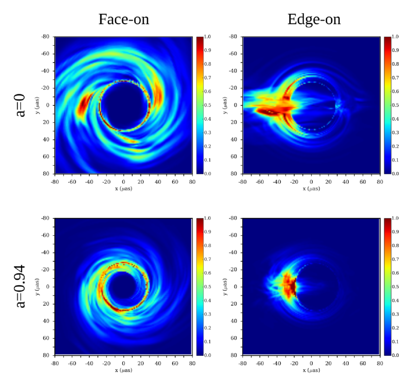
Figure 1: Snapshot of ray-traced images at 1.3 mm for the $a=0$ (upper row) and $a=0.94$ (lower row) simulations. The left and right columns are the face-on and edge-on view images, respectively. The resolution of the images is 128x128. The color scale is linear and normalized.

2.3 Emission Radius

It is convenient to define a characteristic location of emission along each ray, since our hypothesis is that variability along a ray is tightly correlated with its point of emission. Suppose $\lambda$ is the affine parameter along a geodesic. Then

$$\bar{\lambda}\equiv\frac{\int\lambda\left(\frac{\mathrm{d}I}{\mathrm{d}\lambda}\right)^{2}\,\mathrm{d}\lambda}{\int\left(\frac{\mathrm{d}I}{\mathrm{d}\lambda}\right)^{2}\,\mathrm{d}\lambda}$$ (2)

where $I(\lambda)$ is specific intensity. We define the point at $\bar{\lambda}$ along the ray as “emission point”, $\vec{x}(\bar{\lambda})=\vec{x}_{emiss}$; $r(\bar{\lambda})\equiv r_{emiss}$ is the characteristic “emission radius” and $\theta(\bar{\lambda})\equiv\theta_{emiss}$ is the characteristic emission latitude. The bright regions in our model images have $\theta_{emiss}\sim\pi/2$, i.e. the disk’s equatorial plane.

Figure 2 shows $r_{emiss}$ for the face-on and edge-on views of both spins. For the edge-on view, the inner edge of the photon ring has the smallest $r_{emiss}$ (the blue rings in Figure 2). Most of the emission of the rings is from the side and behind the black hole, while the region inside the rings is dominated by emission from gas in front of the black hole; these geodesics extend into the horizon rather than going around the hole. Although the shadow angular radius is insensitive to spin, the range of $r_{emiss}$ that light up the photon ring is strongly dependent on spin: the minimum $r_{emiss}$ in the equatorial plane for the $a=0$ model is $\sim 4.5M$ and becomes $\sim 8M$ as the image position moves $20\,\mu as$ outward, while the same measurement gives $2M$ and $6M$ for the $a=0.94$ model. This introduces a difference in image variability for the two spin models, as discussed in the next subsection.

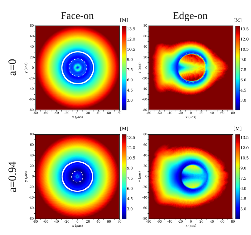
Figure 2: Emission radius, $r_{emiss}$, in $M$ for the $a=0$ (upper row) and $a=0.94$ (lower row) simulations. The left and right columns are the face-on and edge-on view images, respectively. For the face-on images, the region within the dotted white ring is for a low emission from an extended jet region and the $r_{emiss}$ value is not meaningful there. The solid white ring indicates location of the photon ring where the use of our $r_{emiss}$ definition is inadequate (and therefore hidden by the line) for the face-on images.

For the face-on view, emission radius monotonically increases outward from the center of the images except the region inside the white dotted ring. There, a very low emission from extended regions outside the disk (jet) dominates. There is a noticeable difference between the different spin models inside the photon rings, indicated by the solid white rings, where $r_{emiss}$ is smaller by $\sim 1.5-2M$ for the $a=0.94$ model for a given radius from the image center. The use of our $r_{emiss}$ definition in the photon ring is inadequate for the face-on view since light rays penetrate the disk multiple times at different radii as they go around the black hole.

In practice the total intensity in a single pixel is built up from an extended region around its emission point. If this emission region is small, the time variability of the intensity reflects dynamics at the emission point well. If the emission region is large, the variability is built up from variations at multiple locations and it is difficult to extract information from the light curve. Nevertheless, a comparison of Figure 2 with time-domain filtered images that are presented in §3.2 (Figures 4 and 5) shows a strong correlation between the emission radius and time variability in our model images.

3 Time Variability

Is there any feature of the observed emission that constrains the spin of the black hole? Although the brightest region in the image is more extended for the $a=0$ models in Figure 1, image size depends on other model parameters (especially $R$, which can be adjusted until the image size matches the observed value) and does not in itself constrain the spin. The size of the photon ring is very weakly dependent on spin (spin simply moves the centroid of emission at first order in $a$) and thus a constraint on spin will be difficult to extract from photon ring imaging alone.

Is it possible to use time-domain information to constrain the spin? A naive argument suggests that it might be: in our SANE models, the observational variability originates from the orbital motion of turbulent structure in the disk as is discussed below. The variability timescale is thus tied to the orbital timescale, which in turn depends on $r_{emiss}$. For example, emission from the brightest regions in the edge-on views in Figure 1 are generated at $\sim R_{\rm{ph}}<R<2R_{\rm{ISCO}}$, where the corresponding orbital periods for $a=0$ and $a=0.94$ are 6-20 minutes and 12-96 minutes, respectively. We explore below if this relationship between emission radius and orbital period may be detectable in EHT data sets.

3.1 PSD of Total Flux Variability

We begin by examing the power spectrum density (PSD) of the total (source integrated) mm flux. The PSD is constructed as follows. For a light curve $L_{n}$ where $0\leq n\leq N-1$ is the index of the measured point in time and $N$ is the total number of points, its discrete Fourier transform is

$$\tilde{L_{s}}=\sum_{n=0}^{N-1}w_{n}L_{n}e^{2\pi isn/N}$$ (3)

where $-N/2\leq s\leq N/2$ is the index for the temporal frequency and $w_{n}$ is a Hamming window used to reduce the edge artifacts. Then the PSD is defined as

$$P_{s}\equiv\tilde{L_{s}}\tilde{L_{s}^{*}}/W$$ (4)

where $W=N\sum_{n=0}^{N-1}w_{n}^{2}$ (Press et al., 2002). We divide each light curve into 4 segments and average the resultant PSDs where $N\sim 1200$ per segment in our operation. The duration of each segment is $\sim 3.5$ hours (time resolution of our data set is $0.5M\sim 11$ seconds) which is close to the integration time of realistic EHT observation. Averaging over segments also improves the signal-to-noise ratio.

Figure 3 shows the power spectral density (PSD) of the total flux variability for our four models at $a=0,a=0.94$ and $i=0^{\circ},i=90^{\circ}$. The vertical lines indicate the ISCO frequency for $a=0$ (broken) and $a=0.94$ (solid). The total flux in our models comes from an extended range in radius, so its variability is not sensitive to disk dynamics at any particular radius. Overall, edge-on views have higher power in a wide band around the ISCO frequency than face-on views (compare black and red lines of the same line type), while no systematic difference is apparent between different spins with the same viewing angle (compare the same colors).

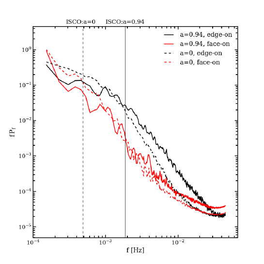
Figure 3: PSD of total flux variability for our models. Solid black, solid red, broken black, and broken red lines are $a=$0.94 edge-on, $a=$0.94 face-on, $a=0$ edge-on, and $a=0$ face-on, respectively. Vertical solid and broken lines indicate ISCO orbital frequency of $a=$0.94 and $a=0$ black hole, respectively. The power is normalized by the maximum value of $a=0$ face-on model.

All the models exhibit a monotonic decrease in power with frequency. There is weak evidence for a break close to the ISCO frequency, with $d\ln P/d\ln f\simeq-2$ below and $d\ln P/d\ln f\gtrsim-3$ above. Observations (Dexter et al., 2014) show an $\sim f^{-2}$ spectrum between $f_{min}\simeq 1.4{\times}10^{-3}$Hz and $f_{max}\simeq 3{\times}10^{-3}$Hz, with a turnover to a flat spectrum at frequencies below $\sim 3.5{\times}10^{-5}$Hz. In a future investigation we will consider the long-timescale behavior and the observed break at $\sim 3.5{\times}10^{-5}$Hz by extending the duration of our simulation. The peak radius of emission in the edge-on views is approximately $5-6M$, but there is still a large contribution to the total flux from smaller radii. The peak emission for face-on views comes from the photon ring (see the left column in Figure 1), but also from a large range in radius. These highly extended origin of emission for the face-on models smear out the variability amplitude and lead to an overall lower power than in edge-on models. Evidently spatially resolved structural variability is essential if we want extract more detailed information about the disk dynamics. However, Figure 3 implies the total flux PSD may allow discrimination between different spin models.

3.2 Time-Domain Filtering of Image

Next, we consider the effects of filtering the mock images in the time domain. We first obtain the light curve of each pixel in Figure 1 and produce a corresponding PSD following the procedure described in §3.1. The PSD is integrated over a frequency band, and the resulting power is assigned to the same pixel to generate a time-domain filtered image. Images reconstructed from observational data will, of course, have coarser angular resolution. After obtaining the sets of PSD of the pixels in the ray-traced images, we analyze their spatial distribution by mapping the power in a band or frequency range $f_{1}<f<f_{2}$; $\mathcal{P}(i,j,f_{1},f_{2})=\int_{f_{1}}^{f_{2}}P(i,j,f)df$ where $i$ and $j$ are the spatial indices of a pixel.

Figures 4 and 5 show unnormalized time-domain filtered images $\mathcal{P}$ for $(f_{1},f_{2})=(10^{-3.8},10^{-3.3})$, $(10^{-2.8},10^{-2.3})$, $(10^{-1.8},10^{-1.3})$ Hz (notice that $f_{\rm{ISCO}}=10^{-2.7}$ and $10^{-3.3}$ Hz for a=0.94 and 0, respectively) together with the time averaged intensity map ($f=0$) for the face-on and edge-on views in a logarithmic color scale. The figures are over-plotted with ellipses to represent the image size and orientation. To obtain these ellipses, we first construct covariance matrix (second moments) of the image pixels and find its eigenvectors and eigenvalues, $\lambda_{1}$ and $\lambda_{2}$. The eigenvectors correspond to the principal axes of the images and their length is the square root of the eigenvalues. The length of the vectors is related to the FWHM of the axisymmetric Gaussian model used for the analysis of VLBI observations by FWHM$/2.3$. The length of the principal axes of the ellipses in Figure 4 and 5 is the FWHM, i.e. $\rm{FWHM}_{1,2}=2.3\sqrt{\lambda_{1,2}}$. The eccentricity of the ellipses $\equiv\sqrt{1-\lambda_{2}/\lambda_{1}}$.

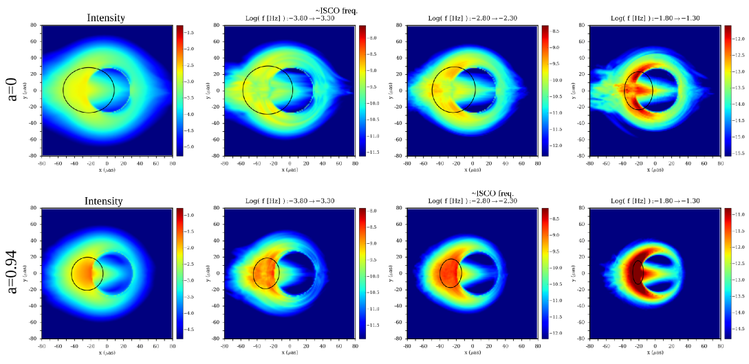
Figure 4: Maps of power in time variability for the edge-on view. The upper and lower rows are for the $a=0$ and $a=0.94$ models, respectively. The columns are for different frequency range that the power is integrated for. The left most column is for $f=0$, i.e. time averaged intensity, and from the second left column to the right most column are, $(f_{1},f_{2})=(10^{-3.8},10^{-3.3})$, $(10^{-2.8},10^{-2.3})$, $(10^{-1.8},10^{-1.3})$ in Hz (ISCO orbital frequencies are $10^{-3.3}$Hz and $10^{-2.7}$Hz for $a=0$ and $a=0.94$, respectively). The color scale is logarithmic and ranged $\rm{Log}(\rm{AVG}[\mathcal{P}(r<40\mu as)])\pm 2$ where $r$ is the distance from the centroid. FOV is the same as Figure 1. The over-plotted ellipses are image size and orientation found from the covariance matrix described in §3.2.

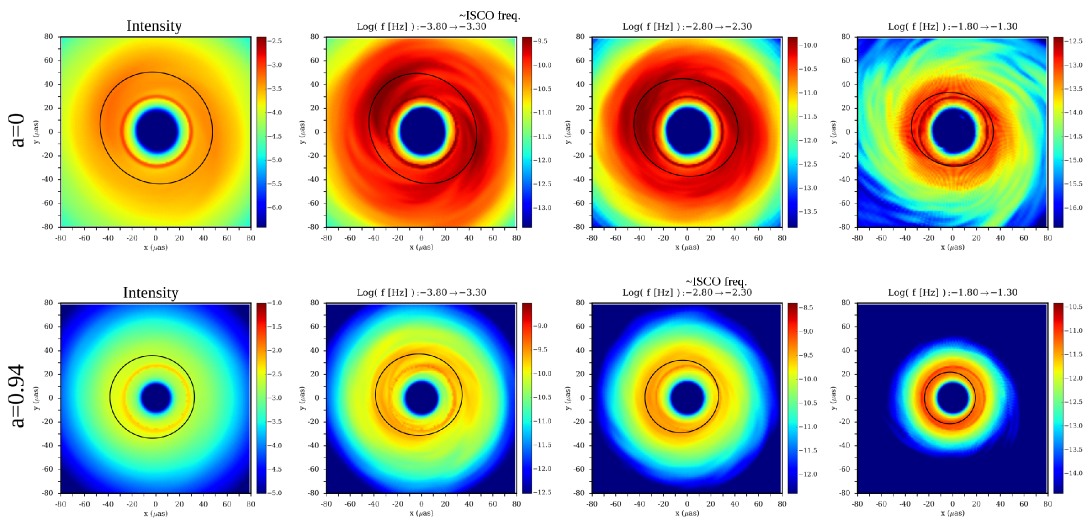
Figure 5: Same as Figure 4 but for the face-on view.

The image size decreases as the filtering frequency increases for all the models in Figures 4 and 5. In general, the smaller $r_{emiss}$, the higher the power at high filtering frequencies and the lower the power at low filtering frequencies, if the intensity is fixed. This naturally arises because the high orbital frequency at the inner radii of the disk produces rapid variability. Emission from large radii has relatively higher power at low filtering frequencies, and hence the image size is larger due to the extended area of emission from outer radii (see Figure 2). On the other hand, emission from small radii occupies a smaller region in the images and the image size gets smaller for high filtering frequencies. This result confirms that our filtering technique is able to visualize a spatial distribution of the local characteristic timescale at $r_{emiss}$. Figure 6 shows the relation between the image size and the filtering frequency range for all the cases where the “size” is the average of FWHM₁ and FWHM₂. The size decreases with increased filter frequency, and ranges from 30% to 50% depending on the model considered.

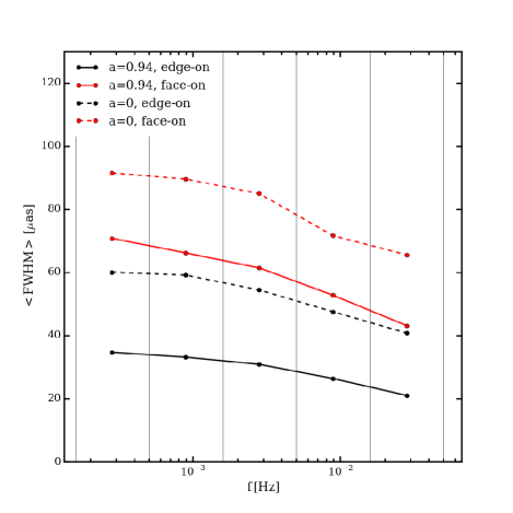
Figure 6: Filtering frequency versus image size of the time-domain filtered images. The vertical lines indicate the filtering frequency range for each plotted points. Solid black, solid red, broken black, and broken red lines are for $a=0.94$ edge-on, $a=0.94$ face-on, $a=0$ edge-on, and $a=0$ face-on, respectively.

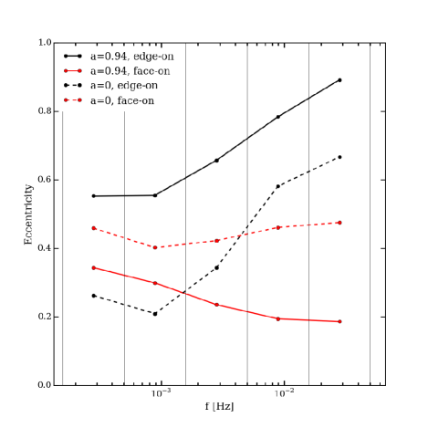
Figure 7: Same as Figure 6 but for the eccentricity of the filtered images.

The high frequency filtered edge-on images (rightmost column in Figure 4) nicely traces the distribution of small emission radii (see Figure 2) for both of the high spin models. This suggests that image eccentricity has a dependence on black hole spin, especially at high filtering frequencies. The eccentricity of the edge-on filtered images in general increases with the filtering frequency, and the high-spin model has higher eccentricity at all the filtering frequencies than the low-spin model; see Figure 7 for the dependence of eccentricity on the filtering frequency. Unlike the edge-on views, eccentricity in the face-on images does not depend much on the filtering frequency. In principle, the degeneracy of spin and viewing angle can be avoided by the unique dependence of eccentricity on the filtering frequency. Surprisingly, face-on images are not always very “round”, as we see the face-on $a=0$ model in Figure 7 has eccentricity $>0.4$ due to the presence of slowly evolving non-axisymmetric structures.

The time-domain filtering technique highlights the direction of the disk’s orbital axis, as the semi-major axis of the ellipses are aligned with it. Even if the black hole shadow is not well resolved or apparent in time-averaged data, filtering at high frequency would show anti-symmetric properties in the variable structure as long as the disk is not viewed face-on. We note that our technique might be used to test if an observed time-averaged feature is a true black hole shadow: if it is, then a similar feature should grow more prominent as the filtering frequency increases.

3.3 Application to EHT Data

Real EHT data is sparsely sampled in the spatial Fourier domain (U-V plane) and has superposed atmospheric and thermal noise as well as interstellar scattering. Thus reconstruction of even static images require sophisticated approaches (e.g. Bouman et al., 2016; Chael et al., 2016). Nevertheless, reconstruction of high time resolution images from incomplete UV-coverage is possible using several newly developed techniques (Johnson et al. 2017, submitted).

We performed a preliminary test to apply the time-domain filtering technique to time variable images produced by a synthetic observation of our high spin edge-on view model, using the array configuration for the EHT 2017 campaign. However, the effects of interstellar scattering and realistic, irregular time sampling (i.e. due to telescopes off-source f or phase calibration) were not included. We found that the technique could reproduce the trend the image size increases and eccentricity decreases as the filtering frequency increases.

3.4 Slow Light and Fast Light

Here, we investigate the effect of using a “fast light” approximation by comparing fast light and slow light time-domain filtered images. Implementation of “slow light” in General Relativistic Ray-tracing code has been done by several researchers (e.g. Dolence et al., 2012, Jason Dexter, personal communication) and it is known to have a significant effects on high frequency variability (Chi-kwan Chan, Thomas Bronzwaer, personal communication).

We found the approximation introduces non-negligible effects on filtered image morphology for the edge-on view, at the high filter frequencies. As an example, Figure 8 shows a comparison of the time filtered images with and without the fast light approximation where the properties of the images are the $a=0.94$ model, edge-on view, and filter frequency range of $10^{-2.3}-10^{-1.8}$Hz (same as the lower row, third column panel in Figure 4 but with a linear color scale). The power around the equatorial plane in the fast light image is approximately 50% less than in the corresponding slow light image. Evidently, the use of slow light is essential for our time-domain filtering technique.

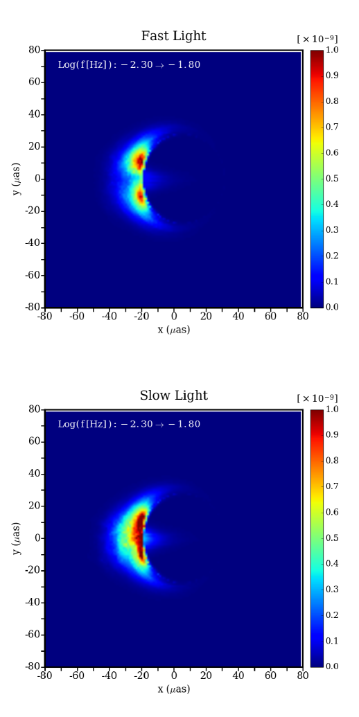
Figure 8: Comparison of the time-domain filtered images calculated using the fast light approximation (upper) and without the approximation (lower). The selected images are for the $a=0.94$ edge-on view model with the filtering frequency range $10^{-2.3}-10^{-1.8}$Hz (ISCO orbital frequency is $\sim 10^{-2.7}$Hz). The color is linearly scaled.

For the same model, the effect of the approximation on the time-domain filtered image is much less apparent at the low filter frequencies, approximately below ISCO orbital frequency $\sim 1.9\times 10^{-3}=10^{-2.7}$Hz. The total flux light curve of the slow light calculation is slightly smoother than that of the fast light but no qualitative difference is apparent.

4 Turbulence and Observed Variability

While numerous simulations of magnetized turbulent accretion disks have been conducted, the resultant turbulence structure depends on the numerical resolution, the initial condition/setting of the simulation, and the physics included in the model (e.g. Hawley et al., 2011; Shiokawa et al., 2012; Kunz et al., 2016; Shi et al., 2016; Ryan et al., 2017). In the absence of clear theoretical guidance, then, it is useful to understand what information time-variable imaging might contain about the structure of turbulence in Sgr A*’s accretion flow. Spatially resolved time-domain data retains information about location specific disk dynamics, which is inaccessible in total flux light curves of Sgr A* that average emission from a broad range of radii in the disk.

Here, we study the relation between the observed light curve for a single pixel and the dynamics of its emission point, $\vec{x}_{emiss}$, to explore how the disk structure at the emission point is translated into the observed variability. We measure time variability of the emissivity at an emission point in the disk’s equatorial plane, obtain its PSD, and then compare this to the PSD obtained from variability of the flux measured in the corresponding pixel. The PSD of the emissivity is obtained using the same method as for the PSD of the flux.

Figure 9 presents PSDs of observed light curves in selected pixels for the face-on $a=$0.94 model, and PSDs of emissivity fluctuations measured at the pixels’ emission points. The selected pixels have their emission radii $r_{emiss}=2M$ and $6M$ in the equatorial plane. Although there are differences in detail between the emissivity and flux PSDs, it is evident that they have remarkably similar shapes, consistent with our suggestion that variability in an image pixel and dynamics at the emission point associated with that region of the image are closely related. This correlation is retained even for pixels that have an extended emission region in the disk such as the brightest region in the edge-on images.

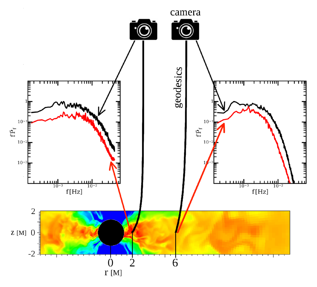
Figure 9: Comparison of observed PSDs in pixels and PSDs of temporal emissivity fluctuation in time measured at the pixels’ emission points $\vec{x}_{emiss}$ in the disk. The selected examples are for pixels that have emission radius $r_{emiss}=2M$ (the left panel) and $6M$ (the right panel) in the equatorial plane for the face-on, $a=0.94$ model. The black PSD curves pointed by the black arrows from the cameras (represent the pixels) are the observed PSDs in the selected pixels, and the red PSD curves pointed by the red arrows from the emission points are the PSDs of emissivity fluctuation measured at those points. The normalizations offset to make both curves visible. Emissivity is average value of 9 grids (3 in radial and 3 in poloidal direction) adjacent to a grid at the emission points. The pseudo-color plot shows density distribution in an example azimuthal and time slice of the accretion disk. The color is logarithmically scaled.

What does the observed PSD tell us about the disk dynamics? The turbulent velocities in the disk are small compared to the orbital speed. This suggests a picture in which the disk fluctuations are regarded as frozen in, and dragged across the line of sight by orbital motion. This implies that the temporal PSD of emissivity at the location is directly connected to the PSD of spatial fluctuation of the emissivity in azimuthal direction. The dominant variability frequency should correspond to the time required for a characteristic turbulent structure to orbit across the line of sight. The characteristic azimuthal size of turbulent structures in the disk is the azimuthal correlation angle $\lambda_{\phi}\ll 2\pi$ (Shiokawa et al., 2012), which corresponds to an azimuthal model number $m=2\pi/\lambda$. Therefore

$$f_{c}(r)\simeq m\frac{\Omega_{p}(r)}{2\pi}\simeq mf_{K}(r)\text{,}$$ (5)

where $\Omega_{p}$ is the pattern speed of the emissivity, which we assume is approximately the Keplerian orbital velocity $f_{K}(r)=[2\pi(r^{3/2}+a)]^{-1}$.

The angular correlation length $\lambda_{\phi}$ of the emissivity in a turbulent disk could be estimated based on the preceding argument. The characteristic mode frequency for the highest mode number $m=2\pi/\lambda_{\phi}$ appears as a break in the PSD; higher frequency fluctuations are weaker because there is comparatively little corresponding small-scale structure in the disk. It turns out that there is a mild break in most of the observed pixel PSDs, including the PSDs in Figure 9, and these breaks correspond to a mode number $m=8-10$, consistent with Shiokawa et al. (2012).

Note that the azimuthal structure of the emissivity strongly on wavelength, as does the synchrotron emissivity (Leung et al., 2011). At shorter wavelength, e.g. in the near infrared, the azimuthal profile is dominated by a few emission spikes rather than by the more smoothly distributed turbulent fluctuations that dominate in the submillimeter. Such spikes could cause Quasi Periodic Oscillations (QPOs) at close to the orbital frequency (Dolence et al., 2012).

5 Summary

The Event Horizon Telescope project is aimed at spatially resolving the mm/submm emission from Sgr A* on scales of a few Schwarzschild radii. Turbulence in the accretion flow surrounding Sgr A* is expected to cause time variability in the sky brightness that can be measured and potentially resolved by EHT. In this paper, we have introduced a time-domain filtering technique that filters time variable images into arbitrary temporal frequency ranges. We have demonstrated the technique’s potential by exploring the connection between the accretion flow and image variability through the use of mock, time-dependent, 1.3mm images based on GRMHD simulations.

By quantifying the image properties using image moments, we find that the filtered images depend strongly on the filter frequency, and make the following predictions:

• Emission from small radii in the disk has rapid variability because it originates from the fastest moving turbulent structures. It appears as relatively concentrated structure in the images and hence the image size at the high filter frequencies are smaller than those low frequencies. The image size decreases with increasing filter frequency for all the parameters we explore ($a=0$ and 0.94, face-on and edge-on viewing angles) by 30-40% for the possible temporal frequency range in the real VLBI observations.

• High frequency filters pick out the photon ring, which is built up from emission close to the photon orbit. Although the size of the photon ring is insensitive to spin, its characteristic variability frequencies are spin dependent because the emission radius (photon orbit radius) is also spin-dependent.

• The filtered image’s eccentricity (a measure of the ellipticity of the image) is spin-dependent in disks seen edge-on. Our models show the edge-on $a=$0.94 model images are more eccentric than the edge-on $a=$0 model at all filter frequencies.

• The filtered image’s major axis is aligned with the spin axis of the black hole and disk. The spin axis can therefore be accessed using our filtering technique.

• The filtered image’s eccentricity is less affected by filter frequency in face-on views. This can be used to differentiate the edge-on and face-on views.

The dependence of the image morphology on filter frequency is a direct consequence of the coupling of disk dynamics to variability. By comparing PSDs, we showed that the flux variability is tightly correlated with the emissivity fluctuations at the point of peak emission along the line of sight. The predominant source of the variability is slowly evolving turbulence structure passing through the emission point at the orbital speed. Therefore, the observed temporal PSD in a pixel is reflection of the spatial PSD of the emissivity turbulent structure at the emission point. This indicates that spatial structure of disk turbulence, and moreover the emission radius distribution in the observational images, are accessible through image variability.

The time filtering approach described here shows that it is possible to directly study black hole spin, viewing angle and spin axis of the Sgr A* system using movies of lensed emission produced by GRMHD simulations. Next steps in this area will include development of algorithms tailored to EHT data sets that aim to estimate these fundamental parameters. Parallel extension of GRMHD simulations to include other effects such as variations in electron/proton temperature ratio in the accretion flow will be useful in application of these techniques to other EHT targets such as M87.

This work was supported by a grant from the National Science Foundation (NSF; AST-1440254) and through an award from the Gordon and Betty Moore Foundation (GBMF-3561). C.F.G. was supported by NSF grant AST-1333612, a Simons Fellowship, and a visiting fellowship at All Souls College, Oxford. C.F.G is also grateful to Oxford Astrophysics for their hospitality. The authors would like to acknowledge Scott Noble for providing GRMHD code HARM3D. We thank Avi Loeb, Pierre Christian, and Michael Johnson for fruitful discussions, and Andrew Chael for assistance in editing the paper.

References

- Baganoff et al. (2001) Baganoff, F. K., Bautz, M. W., Brandt, W. N., et al. 2001, Nature, 413, 45
- Bardeen (1973) Bardeen, J. M. 1973, in Black Holes (Les Astres Occlus), ed. C. Dewitt & B. S. Dewitt, 215–239
- Boehle et al. (2016) Boehle, A., Ghez, A. M., Schödel, R., et al. 2016, ApJ, 830, 17
- Bouman et al. (2016) Bouman, K. L., Johnson, M. D., Zoran, D., et al. 2016, in The IEEE Conference on Computer Vision and Pattern Recognition (CVPR)
- Bower et al. (2005) Bower, G. C., Falcke, H., Wright, M. C., & Backer, D. C. 2005, ApJ, 618, L29
- Bower et al. (2015) Bower, G. C., Markoff, S., Dexter, J., et al. 2015, ApJ, 802, 69
- Broderick et al. (2009) Broderick, A. E., Fish, V. L., Doeleman, S. S., & Loeb, A. 2009, ApJ, 697, 45
- Broderick et al. (2011) —. 2011, ApJ, 735, 110
- Broderick et al. (2016) Broderick, A. E., Fish, V. L., Johnson, M. D., et al. 2016, ApJ, 820, 137
- Chael et al. (2016) Chael, A. A., Johnson, M. D., Narayan, R., et al. 2016, ApJ, 829, 11
- Chan et al. (2015a) Chan, C.-k., Psaltis, D., Özel, F., et al. 2015a, ApJ, 812, 103
- Chan et al. (2015b) Chan, C.-K., Psaltis, D., Özel, F., Narayan, R., & Saḑowski, A. 2015b, ApJ, 799, 1
- Chandra et al. (2015) Chandra, M., Gammie, C. F., Foucart, F., & Quataert, E. 2015, ApJ, 810, 162
- De Villiers et al. (2003) De Villiers, J.-P., Hawley, J. F., & Krolik, J. H. 2003, ApJ, 599, 1238
- Dexter (2016) Dexter, J. 2016, MNRAS, 462, 115
- Dexter et al. (2014) Dexter, J., Kelly, B., Bower, G. C., et al. 2014, MNRAS, 442, 2797
- Dibi et al. (2012) Dibi, S., Drappeau, S., Fragile, P. C., Markoff, S., & Dexter, J. 2012, MNRAS, 426, 1928
- Do et al. (2009) Do, T., Ghez, A. M., Morris, M. R., et al. 2009, ApJ, 691, 1021
- Dodds-Eden et al. (2009) Dodds-Eden, K., Porquet, D., Trap, G., et al. 2009, ApJ, 698, 676
- Doeleman et al. (2009) Doeleman, S., Agol, E., Backer, D., et al. 2009, in Astronomy, Vol. 2010, astro2010: The Astronomy and Astrophysics Decadal Survey
- Doeleman et al. (2008) Doeleman, S. S., Weintroub, J., Rogers, A. E. E., et al. 2008, Nature, 455, 78
- Doeleman et al. (2012) Doeleman, S. S., Fish, V. L., Schenck, D. E., et al. 2012, Science, 338, 355
- Dolence et al. (2009) Dolence, J. C., Gammie, C. F., Mościbrodzka, M., & Leung, P. K. 2009, ApJS, 184, 387
- Dolence et al. (2012) Dolence, J. C., Gammie, C. F., Shiokawa, H., & Noble, S. C. 2012, ApJ, 746, L10
- Eckart et al. (2008) Eckart, A., Schödel, R., García-Marín, M., et al. 2008, A&A, 492, 337
- Fish et al. (2011) Fish, V. L., Doeleman, S. S., Beaudoin, C., et al. 2011, ApJ, 727, L36
- Fish et al. (2016) Fish, V. L., Johnson, M. D., Doeleman, S. S., et al. 2016, ApJ, 820, 90
- Fishbone & Moncrief (1976) Fishbone, L. G., & Moncrief, V. 1976, ApJ, 207, 962
- Foucart et al. (2016) Foucart, F., Chandra, M., Gammie, C. F., & Quataert, E. 2016, MNRAS, 456, 1332
- Gammie et al. (2003) Gammie, C. F., McKinney, J. C., & Tóth, G. 2003, ApJ, 589, 444
- Genzel et al. (2003) Genzel, R., Schödel, R., Ott, T., et al. 2003, Nature, 425, 934
- Ghez et al. (2008) Ghez, A. M., Salim, S., Weinberg, N. N., et al. 2008, ApJ, 689, 1044
- Gold et al. (2017) Gold, R., McKinney, J. C., Johnson, M. D., & Doeleman, S. S. 2017, ApJ, 837, 180
- Haubois et al. (2012) Haubois, X., Dodds-Eden, K., Weiss, A., et al. 2012, A&A, 540, A41
- Hawley et al. (2011) Hawley, J. F., Guan, X., & Krolik, J. H. 2011, ApJ, 738, 84
- Hornstein et al. (2007) Hornstein, S. D., Matthews, K., Ghez, A. M., et al. 2007, ApJ, 667, 900
- Johannsen et al. (2016) Johannsen, T., Broderick, A. E., Plewa, P. M., et al. 2016, Physical Review Letters, 116, 031101
- Johnson et al. (2015) Johnson, M. D., Fish, V. L., Doeleman, S. S., et al. 2015, Science, 350, 1242
- Kunz et al. (2016) Kunz, M. W., Stone, J. M., & Quataert, E. 2016, Physical Review Letters, 117, 235101
- Leung et al. (2011) Leung, P. K., Gammie, C. F., & Noble, S. C. 2011, ApJ, 737, 21
- Lu et al. (2016) Lu, R.-S., Roelofs, F., Fish, V. L., et al. 2016, ApJ, 817, 173
- Luminet (1979) Luminet, J.-P. 1979, A&A, 75, 228
- Marrone et al. (2008) Marrone, D. P., Baganoff, F. K., Morris, M. R., et al. 2008, ApJ, 682, 373
- Medeiros et al. (2016) Medeiros, L., Chan, C.-k., Ozel, F., et al. 2016, ArXiv e-prints, arXiv:1601.06799
- Medeiros et al. (2017) Medeiros, L., Chan, C.-k., Özel, F., et al. 2017, ApJ, 844, 35
- Meyer et al. (2009) Meyer, L., Do, T., Ghez, A., et al. 2009, ApJ, 694, L87
- Mościbrodzka et al. (2014) Mościbrodzka, M., Falcke, H., Shiokawa, H., & Gammie, C. F. 2014, A&A, 570, A7
- Mościbrodzka et al. (2009) Mościbrodzka, M., Gammie, C. F., Dolence, J. C., Shiokawa, H., & Leung, P. K. 2009, ApJ, 706, 497
- Narayan et al. (2012) Narayan, R., SÄ dowski, A., Penna, R. F., & Kulkarni, A. K. 2012, MNRAS, 426, 3241
- Narayan & Yi (1994) Narayan, R., & Yi, I. 1994, ApJ, 428, L13
- Narayan et al. (2016) Narayan, R., Zhu, Y., Psaltis, D., & Saḑowski, A. 2016, MNRAS, 457, 608
- Neilsen et al. (2013) Neilsen, J., Nowak, M. A., Gammie, C., et al. 2013, ApJ, 774, 42
- Noble et al. (2006) Noble, S. C., Gammie, C. F., McKinney, J. C., & Del Zanna, L. 2006, ApJ, 641, 626
- Noble et al. (2009) Noble, S. C., Krolik, J. H., & Hawley, J. F. 2009, ApJ, 692, 411
- Noble et al. (2007) Noble, S. C., Leung, P. K., Gammie, C. F., & Book, L. G. 2007, Classical and Quantum Gravity, 24, 259
- Porquet et al. (2008) Porquet, D., Grosso, N., Predehl, P., et al. 2008, A&A, 488, 549
- Press et al. (2002) Press, W. H., Teukolsky, S. A., Vetterling, W. T., & Flannery, B. P. 2002, Numerical recipes in C++ : the art of scientific computing
- Psaltis et al. (2015) Psaltis, D., Özel, F., Chan, C.-K., & Marrone, D. P. 2015, ApJ, 814, 115
- Ressler et al. (2015) Ressler, S. M., Tchekhovskoy, A., Quataert, E., Chandra, M., & Gammie, C. F. 2015, MNRAS, 454, 1848
- Ryan et al. (2017) Ryan, B. R., Gammie, C. F., Fromang, S., & Kestener, P. 2017, ApJ, 840, 6
- Schnittman & Krolik (2013) Schnittman, J. D., & Krolik, J. H. 2013, ApJ, 777, 11
- Shcherbakov & McKinney (2013) Shcherbakov, R. V., & McKinney, J. C. 2013, ApJ, 774, L22
- Shi et al. (2016) Shi, J.-M., Stone, J. M., & Huang, C. X. 2016, MNRAS, 456, 2273
- Shiokawa et al. (2012) Shiokawa, H., Dolence, J. C., Gammie, C. F., & Noble, S. C. 2012, ApJ, 744, 187
- Trap et al. (2011) Trap, G., Goldwurm, A., Dodds-Eden, K., et al. 2011, A&A, 528, A140
- White et al. (2016) White, C. J., Stone, J. M., & Gammie, C. F. 2016, ApJS, 225, 22
- Yusef-Zadeh et al. (2009) Yusef-Zadeh, F., Bushouse, H., Wardle, M., et al. 2009, ApJ, 706, 348