Exact solution of a classical short-range spin model with a phase transition in one dimension: the Potts model with invisible states

Abstract

We present the exact solution of the 1D classical short-range Potts model with invisible states. Besides the $q$ states of the ordinary Potts model, this possesses $r$ additional states which contribute to the entropy, but not to the interaction energy. We determine the partition function, using the transfer-matrix method, in the general case of two ordering fields: $h_{1}$ acting on a visible state and $h_{2}$ on an invisible state. We analyse its zeros in the complex-temperature plane in the case that $h_{1}=0$. When ${\rm Im}\,h_{2}=0$ and $r\geq 0$, these zeros accumulate along a line that intersects the real temperature axis at the origin. This corresponds to the usual “phase transition” in a $1$D system. However, for ${\rm Im}\,h_{2}\neq 0$ or $r<0$, the line of zeros intersects the positive part of the real temperature axis, which signals the existence of a phase transition at non-zero temperature.

1 Introduction

Few models in statistical physics can be solved exactly and many of those that can are in a single dimension [1]. Knowing the behaviour of a system in one dimension (1D) can help one to understand and predict its behaviour in higher dimensions too. Also some chemical compounds are effectively described by quasi-1D models [2, 3, 4, 5, 6]. For these reasons, 1D models are interesting from both theoretical and experimental points of view.

In the 1920s Wilhelm Lenz and Ernst Ising suggested and investigated the first microscopic model of ferromagnetism [7, 8]. Theirs involved a one-dimensional lattice occupied by classical spins which can only be in one of two states: up or down. In the short-range version, only nearest neighboring spins are allowed to interact. Ising showed that this model has no phase transition at any physically accessible (i.e., non-zero) temperature $T$ [8]. This served as the first and archetypal example of the absence of a finite-$T$ phase transition in 1D classical systems with short-range interactions [9]. Later, in their famous book [10], Landau and Lifshitz gave a heuristic argument that for classical systems there is no phase transition at non-zero temperature in 1D. The approach is based on separately evaluating contributions to the free energy $F=E-TS$ coming from the interaction energy $E$ and the entropy $S$. For the Ising model there are two ground states in which all spins are either up or down. At zero temperature the system is in one of these states. At finite temperatures, domain walls separate regions of up- and down-spins. Each domain wall “costs” energy (i.e., it increases the interaction energy $E$). But in the 1D case this is outweighed by the entropic contribution coming from the number of ways of placing domain walls on the chain. See, e.g., Ref.[11] where it is explicitly shown that adding domain walls reduces the free energy. Therefore, at any temperature it is energetically favourable for domain walls to be inserted. This means the system cannot become ordered and there is no phase transition in such 1D systems.

van Hove proved the absence of a phase transition in one-dimensional fluid-like systems of particles with non-vanishing incompressibility radius and a finite range of forces [12]. This was extended by Ruelle [13] to lattice models. These results are based on the Perron-Frobenius theorem [14]. However, and as emphasised by Cuesta and Sánchez, none of these theorems preclude the existence of thermodynamic phase transitions in general 1D systems with short-range interactions [15]. Indeed Cuesta and Sánchez gave examples of such models and Theodorakopoulos also discussed how the no-go theorems might be circumvented [16]. Ref. [17] maps the 1D multispin-interaction Ising model in a field onto a zero-field 2D Ising model with nearest neighbours interaction. Additionally, quantum 1D models offer further examples of systems which can undergo a phase transition at non-zero temperatures because they are related to 2D classical systems [18].

In the light of these enduring discussions, it is interesting to investigate further circumstances in which classical systems might exhibit a phase transition in 1D. In particular, we are interested in a mechanism in which entropy production can be suppressed in order to sidestep the conditions of the arguments and theorems discussed above. To do so we consider the Potts model with invisible states which was introduced a few years ago [19, 20] in order to explain some questions about the order of a phase transition where $Z(3)$ symmetry is broken. It differs from the ordinary Potts model [21, 22] by adding non-interacting states; if a spin is in one such state, it is “invisible” to its neighbours. Originally, the corresponding Hamiltonian was written in the form

$$H=-\sum_{<i,j>}\delta_{S_{i},S_{j}}\sum_{\alpha=1}^{q}\delta_{S_{i},\alpha}\delta_{S_{j},\alpha},$$ (1)

where $q$ and $r$ are the number of visible and invisible states of the Potts variable

$$s_{i}=1,\ldots,q,q+1,\ldots,q+r\,.$$ (2)

The first sum in (1) is taken over all distinct pairs of interacting particles, and the second sum requires both of the interacting spins to be in the same visible state. From now and on we will use the notation $(q,r)$-state Potts model for model with $q$ visible and $r$ invisible states.

In the ordinary Potts model [21], the parameter $q\geq 2$ has been introduced as an integer denoting the number of (visible) states that a site can be in. However, it has been extended to other values too in order to describe bond percolation ($q=1$), dilute spin glasses ($q=1/2$), and gelation ($q=0$) [22, 23, 24]. The parameter $q$ has been extended to complex values as well [25, 26, 27, 28]. In a similar way, although an initial interpretation of the parameter $r$ is the number of invisible states, we extend it here to non-integer and even negative values. As we will show below, the latter corresponds to removing entropy from the system and will be key to inducing a phase transition.

Adding invisible states does not change the spectrum of the model, it only changes the degeneracy of energy levels (the number of configurations with a given energy). Even though invisible states do not change the interaction energy, since they change the entropy they affect the free energy. As a consequences, for example, an increase in the number $r$ of invisible states may cause a phase transition to change from second to first order [19, 29]. For example the $(2,30)$-state model on a square lattice undergoes the first order transition, while the ordinary $(2,0)$-state Potts model (i.e. the Ising model) is an iconic example of a continuous transition.

The Potts model with invisible states describes a number of models of physical interest. In particular, the $(1,r)$-state model can be mapped to the Ising model in a temperature-dependent field [30]. The 1D $(1,r)$ case with nearest-neighbour interactions is equivalent to the Zimm-Bregg model for the helix-coil transition [30]. The multi-spin extension of this model possesses a re-entrant phase transition and is in good agreement with experimental observations for polymer transitions [31, 32]. The $(2,r)$-state Potts model without external fields is equivalent to the Blume–Emery–Grifiths (BEG) model [19, 33, 34] with a temperature dependent external field. Furthermore, the general $q$ and $r$ case can be interpreted as a diluted Potts model [19, 29]

$$H^{\prime}=-\sum_{<i,j>}\delta_{\sigma_{i},\sigma_{j}}(1-\delta_{\sigma_{i},0})-T\ln r\sum_{i}\delta_{\sigma_{i},0},$$ (3)

where $\sigma_{i}=0,1,\ldots,q$ is a new spin variable and all invisible states are gathered into one the zeroth state $\sigma_{i}=0$.

In this paper we perform an analysis of the partition function zeros to obtain the exact solution for the 1D Potts model with invisible states. In achieving this, we add another exact result to the existing collection of exactly solved models in statistical mechanics. As we will show below, although one-dimensional, the model manifests a second order transition at non-zero temperature provided some unusual conditions are assumed. We will discuss regimes in which such behaviour is observed and a possible connection with quantum systems.

The rest of the paper is organised as follows: in Section 2 we present the exact solution using the transfer-matrix method, then in Section 3 the existence of a phase transition at non-zero temperature is demonstrated using partition function zeros, and finally conclusions are given in Section 4.

2 Exact solution of the Potts model with invisible states

Let us consider the $(q,r)$-state Potts model on a chain consisting of $N$ spins with only nearest-neighbour interactions subject to two separate magnetic fields $h_{1}$ and $h_{2}$ acting on the first visible and the first invisible states respectively. Imposing periodic boundary conditions, the Hamiltonian of such a system may be written as

$$H_{(q,r)} = -\sum_{i}\sum_{\alpha=1}^{q}\delta_{s_{i},\alpha}\delta_{\alpha,s_{i+1}}$$ (4)

$$-h_{1}\sum_{i}\delta_{s_{i},1}-h_{2}\sum_{i}\delta_{s_{i},q+1}\,,$$

where the sum over $i$ is taken over all sites of the chain.

We will use the transfer matrix formalism [35, 36, 37] to obtain the exact solution of the model (4). The Hamiltonian (4) can be expressed as a sum of terms representing one bond each, so that $H_{(q,r)}=\sum_{i}H_{i}$ where

$$H_{i}=-\sum_{\alpha=1}^{q}\delta_{s_{i},\alpha}\delta_{\alpha,s_{i+1}}-h_{1}\delta_{s_{i},1}-h_{2}\delta_{s_{i},q+1}\,.$$ (5)

Then the partition function can be transformed to

$$Z=\sum_{s}\exp\left[{-\beta H_{(q,r)}}\right]=\sum_{s}\prod_{i}\exp\left(-\beta H_{i}\right)\,.$$ (6)

where $\beta=1/kT$ and $k$ is the Boltzmann constant. Now it is easy to define the $(q+r)\times(q+r)$ square transfer matrix with elements

$$T_{ij}=\exp\left[{\beta\left({\delta_{s_{i},s_{j}}\sum_{\alpha=1}^{q}\delta_{s_{i},\alpha}+h_{1}\delta_{s_{i},1}+h_{2}\delta_{s_{i},q+1}}\right)}\right].$$ (7)

Let us denote

$$t=e^{-\beta}\,,\,z_{1}=e^{\beta h_{1}}\,,\,z_{2}=e^{\beta h_{2}}\,.$$ (8)

With this notation, positive values of temperature $T$ correspond to $t$ ranging from zero to one, and the elements of the transfer matrix can be written in the compact form: $T_{11}=z_{1}/t$; $T_{ii}=t^{-1}$ for $1<i\leq q$; $T_{i1}=z_{1}$; $T_{(q+1)i}=z_{2}$; and all remaining elements equal to $1$.

Based on the transfer-matrix symmetry it is easy to show that it has five different eigenvalues. The eigenvalue $\lambda_{0}=0$ is $(r-1)$ times degenerate because the final $r$ columns of the matrix are proportional. Because $(q-1)$ elements of the main diagonal are equal to $t^{-1}$, choosing $\lambda=t^{-1}-1$ one can find $q-2$ linear independent eigenvectors. This reduces the problem to the determination of three more eigenvalues. They can be found using invariant permutations. The above considerations lead to the equation for the three remaining eigenvalues:

$$(r+z_{2}-1-\lambda)[(\frac{1}{t}-1)z_{1}-\lambda][(\frac{1}{t}-1)-\lambda]$$

$$-\lambda z_{1}[(\frac{1}{t}-1)-\lambda]-(q-1)\lambda[(\frac{1}{t}-1)z_{1}-\lambda]=0\,.$$ (9)

This equation is of third order and can be solved exactly. Since the partition function is [35, 36, 37]

$$Z=\lambda_{1}^{N}+\lambda_{2}^{N}+\lambda_{3}^{N}+\lambda_{4}^{N},$$ (10)

and all the $\lambda$’s have been found, the problem has been solved exactly. In the thermodynamic limit $N\to\infty$ only the largest eigenvalue contributes to the partition function.

It is worth mentioning that the number of invisible states $r$ and the magnetic field $z_{2}$ appear as an additive combination in Eq.(2); the factor $r+z_{2}-1$ can be treated as a temperature-dependent effective number of invisible states.

3 Partition function zeros

Critical properties of any system can be recovered from its partition function. In the transfer-matrix approach, this is expressed in terms of the transfer-matrix eigenvalues as in Eq.(10). Since all the $\lambda$’s can be found explicitly for the Potts model with invisible states, its thermodynamic properties can be found explicitly as well. Eq. (2) is of third order, making the exact solution cumbersome. Analysis of the partition-function zeros in the complex temperature plain (Fisher zeros) ameliorate this problem [38]. In the thermodynamic limit they approach the real axis at the transition point. For the 1D system, Fisher zeros can be obtained by equating (at least) the two eigenvalues which are largest by modulus [39, 5, 6]:

$$|\lambda_{1}|=|\lambda_{2}|>|\lambda_{3}|,\,|\lambda_{4}|\,.$$ (11)

It is clear from this condition that $\lambda_{2}=e^{i\phi}\lambda_{1}$, where $\phi$ is a real phase factor. Then the partition function (10) attains the form

$$Z=|\lambda_{1}|^{N}\left[{1+e^{iN\phi}+\left(\frac{\lambda_{3}}{\lambda_{1}}\right)^{N}+\left(\frac{\lambda_{4}}{\lambda_{1}}\right)^{N}}\right].$$ (12)

In the thermodynamic limit the third and the forth terms in the brackets are negligible and thus the phase $\phi$ is not arbitrary but can take only the values $\phi=(2k-1)\pi/N$, where $k=1\dots N$.

Consider first the case $h_{1}=h_{2}=0$ (i.e. $z_{1}=z_{2}=1$). This reduces the number of eigenvalues in (10) and only three non-zero eigenvalues remain. A typical plot of Fisher zeros that follows from Eqs. (11) and (12) is shown in Figure 1. As one can see from the plot, the zeros approach the real axis at the point $t=0$, which corresponds to the zero-temperature phase transition.

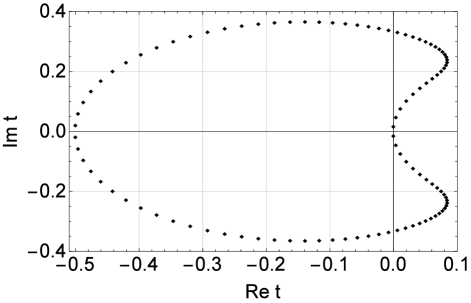
Figure 1: Fisher zeros for the (2,2)-state Potts model for system size $N=100$ in the complex $t$–plane. Here $h_{1}=h_{2}=0$. The zeros approach the real $t$-axis at the point corresponding to the phase transition, namely at $t=0$ ($T=0$).

The question that concerns us here is: what are the circumstances in which the locus of Fisher zeros corresponds to a phase transition at non-zero temperature in 1D? In the following, we discuss two cases where such behaviour is observed.

3.1 The case $h_{1}=0$, $h_{2}\in{C}$

We first demonstrate that when the field $h_{1}$ is zero, such behaviour can be achieved by allowing field $h_{2}$ to be complex. To this end we set the discriminant of Eq. (2) equal to zero for positive temperature and $h_{1}=0,h_{2}\in{C}$. This leads to a relation between the critical temperature and field $h_{2}$, namely

$$z_{2}=t^{-1}-q-r\pm 2i\sqrt{q(t^{-1}-1)}\,.$$ (13)

In this equation, the temperature resides in $t$ and in $z_{2}=t^{-h_{2}}$. For a given (real) value of $t$ between $0$ and $1$ [$T\in(0,\infty)$], we numerically obtain complex values for $h_{2}=\rm{Re}\,h_{2}+i{\rm{Im}}\,h_{2}$. We plot these values in the form $e^{-h_{2}}$ in Fig.2 for the example where $q=2$, $r=3$. Every strictly complex point on the plot corresponds to a positive real value of $T$.

The resulting plot has a form of the double spiral, two branches of the spiral correspond to two complex conjugate values of the field.

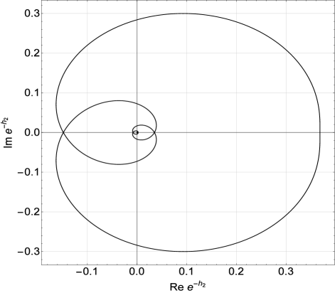
Figure 2: Values of $e^{-h_{2}}$, for which the phase transition in the (2,3)-state Potts model occurs at positive temperature. Each point of the plot corresponds to a certain physically accessible critical temperature.

Obviously, the variable $h_{2}$ does not have a direct, real physical interpretation; it is a complex field acting on invisible states. As expected, the finite-temperature phase transition does not occur in the 1D system under real physical conditions [10, 13]. However, it was recently suggested that the complex magnetic field in a classical system can be mapped onto decoherence time [40] in its quantum counterpart [40]. Of course, in quantum systems finite-temperature phase transitions are allowed, even in 1D [18]. Effectively, rendering the field $h_{2}$ complex, as was done above, adds additional degrees of freedom to the system. Similarly, an increase of the number of degrees of freedom occurs when one passes from a classical to a quantum description. In this sense, the phase transition described above, although occurring in an unphysical region of parameter space, may have a counterpart in the quantum world. Moreover, the external field $h_{2}$ can be tuned to change the system’s behaviour from quantum into classical and vice versa.

3.2 The case $h_{1}=0$, $h_{2}=0$ and $r<0$

Another way to invoke a phase transition is to relax the condition of positivity on the number of invisible states $r$. As we noted before, the free energy of the one-dimensional system with two mixed phases decreases with increasing the number of domain walls, so that an ordering phase transition is not possible for finite temperature [10]. As a way to circumvent this restriction one can try to introduce a mechanism that leads to entropy decrease and therefore to the free energy increase. The calculations displayed below are based on the obvious observation that if adding invisible states increases the entropy, a negative number of invisible states decreases it.

To demonstrate the behaviour of the Potts model with a negative number of invisible states, in Figure 3 we display Fisher zeros for the (2,-6)-state Potts model.

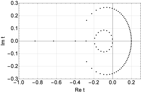
Figure 3: Fisher zeros for the (2,-6)-state Potts model for system size $N=100$ in the complex $t$–plane. The Fisher zeros cross the real axis at the point $t=0.2$ corresponding to a physical temperature of $T=0.621$.

As one can see from the figure, the locus of Fisher zeros in this case intersects the real axis at a positive value of the temperature $t$. The equivalent representation of the Potts model with invisible states through Eq. (3) indicates that the chemical potential is $\mu=-T\log r$. Therefore the negative number of invisible states is equivalent to a model with complex chemical potential. Again, via the aforementioned relation between the complex external field and decoherence time [40], this gives a connection to the behaviour of quantum systems.

Although both methods introduced above can shift the critical point from zero to positive values, the order of the phase transition and the values of the critical exponents remain the same as for the 1D Ising model, namely $\nu=1,\,\alpha=1,\,\eta=1,\,\gamma=1,\,\mu=0,\,\beta=0,\,\delta=\infty$ [1].

4 Conclusions

One dimensional models of statistical physics are interesting from both theoretical and experimental points of view, often opening the way to develop methods for solving more complex problems. In this paper we exactly solved the Potts model with invisible states with two ordering fields in 1D using the transfer-matrix method.

Various authors gave arguments and theorems delivering the absence of positive-temperature phase transitions in classical 1D systems [10, 12, 13, 15]. These can only exhibit properties characteristic of second-order phase transitions at zero temperature [1]. Here we introduced two methods to circumvent these arguments and theorems to induce phase transitions at physically accessible temperatures in a 1D short-range system.

The first method involves placing the system into a complex external field acting on an invisible state. This method allows one to achieve any critical temperature by tuning of the field. In recent publications it was shown that a complex external field for a classical system can be mapped to the decoherence time of a quantum counterpart system [40]. Thus allowing the external field to be complex might be interpreted as giving a classical system certain quantum properties.

The second method we have introduced here involves using negative numbers of invisible states $r$. This way may be interpreted as introducing some ordering factor to the system, reducing its entropy. An alternative interpretation is in terms of a complex chemical potential.

The reason why rigorous theorem proved in [13] doesn’t hold here lies in the fact, that the proof was made using Perron-Frobenius theorem, which is applicable only for matrices of real positive values. Once either the external field or the chemical potential becomes complex, this statement, in general, is not true. Regarding the arguments given by Landau and Lifshitz, it concerns systems which tend to the state with free energy minimum. For complex values of parameters, energy becomes complex as well, and for complex numbers minimum is not defined.

These results offer further counter-examples to the often asserted general statement that there can be no positive-temperature phase transitions in 1D systems with short-range interactions. Indeed, and as convincingly pointed out in Ref.[15], although 1D systems are very thoroughly researched, they are still capable of yielding exciting new physics.

Acknowledgements: We would like to thank Nerses Ananikian and Vahan Hovhannisyan for fruitful discussions. This work was supported in part by FP7 EU IRSES projects No. 612707 “Dynamics of and in Complex Systems” and No. 612669 “Structure and Evolution of Complex Systems with Applications in Physics and Life Sciences”.

References

- [1] Baxter, R. J. (1982). Exactly solved models in statistical physics. Academic, New York.
- [2] Azuma, M., Hiroi, Z., Takano, M., Ishida, K., and Kitaoka, Y. (1994). Physical review letters, 73, 3463.
- [3] Rice, T. M., Gopalan, S., and Sigrist, M. (1993). EPL (Europhysics Letters), 23, 445.
- [4] Schulz, H. J. (1986). Physical Review B, 34, 6372.
- [5] Ghulghazaryan, R. G., Sargsyan, K. G., and Ananikian, N. S. (2007). Physical Review E, 76, 021104.
- [6] Hovhannisyan, V. V., Ghulghazaryan, R. G., and Ananikian, N. S. (2009). Physica A: Statistical Mechanics and its Applications, 388, 1479.
- [7] Lenz, W. (1920). Zeitschrift für Physik, 21, 613.
- [8] Ising, E. (1925). Zeitschrift für Physik, 31, 253.
- [9] Ising T., Folk R., Kenna R., Berche B., and Holovatch Yu. (2017) preprint arXiv:1706.01764.
- [10] Landau, L. D., and Lifshitz, E. M. (1969). Statistical Physics: V. 5: Course of Theoretical Physics. Pergamon press.
- [11] Christensen, K., and Moloney, N. R. (2005). Complexity and criticality. Imperial College Press.
- [12] van Hove, L. (1950). Physica, 16(2), 137.
- [13] Ruelle, D. (1969). Rigorous results in statistical mechanics. Lectures in Theoretical Physics.
- [14] Gantmacher, F. R. (1959). Matrix Theory. Chelsea, New York.
- [15] Cuesta, J. A., and Sánchez, A. (2004). Journal of statistical physics, 115, 869.
- [16] Theodorakopoulos, N. (2006). Physica D: Nonlinear Phenomena, 216, 185.
- [17] Turban, L. (2016). Journal of Physics A: Mathematical and Theoretical, 49, 355002.
- [18] Suzuki, M. (1976). Progress of theoretical physics, 56, 1454.
- [19] Tamura, R., Tanaka, S., and Kawashima, N. (2010). Progress of theoretical physics, 124, 381.
- [20] Tanaka, S., and Tamura, R. (2011). Journal of Physics: Conference Series, 320, 012025.
- [21] Potts, R. B. (1952). Mathematical proceedings of the Cambridge philosophical society, 48, 106.
- [22] Wu, F. Y. (1982). Reviews of modern physics, 54, 235.
- [23] Aharony, A., and Pfeuty, P. (1979). Journal of Physics C: Solid State Physics, 12, L125.
- [24] Lubensky, T. C., and Isaacson, J. (1978). Physical Review Letters, 41, 829.
- [25] Glumac, Z., and Uzelac, K. (2002). Physica A: Statistical Mechanics and its Applications, 310, 91.
- [26] Chang, S. C., and Shrock, R. (2013). Physics Letters A, 377, 671.
- [27] Kim, S. Y., and Creswick, R. J. (2001). Physical Review E, 63, 066107.
- [28] Kim, S. Y. (2004). Journal of the Korean Physical Society, 45, 302.
- [29] Krasnytska, M., Sarkanych, P., Berche, B., Holovatch, Y., and Kenna, R. (2016). Journal of Physics A: Mathematical and Theoretical, 49, 255001.
- [30] Badasyan, A. V., Giacometti, A., Mamasakhlisov, Y. S., Morozov, V. F., and Benight, A. S. (2010). Physical Review E, 81, 021921.
- [31] Badasyan, A. V., Tonoyan, S. A., Mamasakhlisov, Y. S., Giacometti, A., Benight, A. S., and Morozov, V. F. (2011). Physical Review E, 83, 051903.
- [32] Badasyan, A., Tonoyan, S., Giacometti, A., Podgornik, R., Parsegian, V. A., Mamasakhlisov, Y., and Morozov, V. (2012). Physical review letters, 109, 068101.
- [33] Johnston, D. A., and Ranasinghe, R. P. K. C. M. (2013). Journal of Physics A: Mathematical and Theoretical, 46, 225001.
- [34] Ananikian, N., Izmailyan, N. S., Johnston, D. A., Kenna, R., and Ranasinghe, R. P. K. C. M. (2013). Journal of Physics A: Mathematical and Theoretical, 46, 385002.
- [35] Katsura, S., and Ohminami, M. (1972). Journal of Physics A: General Physics, 5, 95.
- [36] Kim, S. Y., and Creswick, R. J. (2000). Physica A: Statistical Mechanics and its Applications, 281, 252.
- [37] Shrock, R., and Tsai, S. H. (1997). Physical Review E, 55, 5184.
- [38] Fisher, M. E. (1964). Lectures in Theoretical Physics: Volume VII. University of Colorado, Boulder.
- [39] Fisher, M. E. (1980). Progress of Theoretical Physics Supplement, 69, 14.
- [40] Wei, B. B., and Liu, R. B. (2012). Physical review letters, 109, 185701; Peng, X., Zhou, H., Wei, B. B., Cui, J., Du, J., and Liu, R. B. (2015). Physical review letters, 114, 010601.