The Fundamental Stellar Parameters of FGK Stars in the SEEDS Survey

Abstract

Large exoplanet surveys have successfully detected thousands of exoplanets to-date. Utilizing these detections and non-detections to constrain our understanding of the formation and evolution of planetary systems also requires a detailed understanding of the basic properties of their host stars. We have determined the basic stellar properties of F, K, and G stars in the Strategic Exploration of Exoplanets and Disks with Subaru (SEEDS) survey from echelle spectra taken at the Apache Point Observatory’s 3.5m telescope. Using ROBOSPECT to extract line equivalent widths and TGVIT to calculate the fundamental parameters, we have computed $T_{eff}$, $log(g)$, $v_{t}$, $[Fe/H]$, chromospheric activity, and the age for our sample. Our methodology was calibrated against previously published results for a portion of our sample. The distribution of $[Fe/H]$ in our sample is consistent with that typical of the Solar neighborhood. Additionally, we find the ages of most of our sample are $<500Myrs$, but note that we cannot determine robust ages from significantly older stars via chromospheric activity age indicators. The future meta-analysis of the frequency of wide stellar and sub-stellar companions imaged via the SEEDS survey will utilize our results to constrain the occurrence of detected co-moving companions with the properties of their host stars.

1 Introduction

Since the discovery of the first exoplanet surrounding a Sun-like star (Mayor & Queloz, 1995), dedicated planet surveys such as, those utilizing the Kepler Space Telescope (Borucki et al., 2009, 2010, 2011), the California Planet Search (Howard et al., 2010; Wright et al., 2011) and the Anglo-Australian Telescope planet search (Tinney et al., 2001; Butler et al., 2001; Wittenmyer et al., 2014) have expanded the number of confirmed exoplanets to-date to more than $\sim$3,000 exoplanets (exoplanets.org). These surveys have yielded sufficient numbers of detections to enable correlations with their host star properties, such as mass and metallicity, to better constrain our understanding of how planets form.

A variety of studies have sought to identify trends between the frequency of exoplanets and a given host star’s fundamental parameters. Shortly after the first detections of exoplanets, it was recognized that there was a trend between the occurrence of Jovian-mass exoplanets and their host star metallicity (eg. Gonzalez 1997; Fischer & Valenti 2005). More recently, this relation has been extended for Jovian-mass planets surrounding intermediate mass sub-giants to M-dwarf hosts Johnson et al. (2010) and to terrestrial-size exoplanets (R$<$1.7 R_Earth) (Wang & Fischer, 2015). Jovian mass planets are seen to increase in frequency around their host stars from M-dwarf stars to A-dwarfs stars (Johnson et al., 2010). It has also been suggested that the frequency of planets varies inversely with the lithium abundance of the host star (Israelian et al., 2009), though this trend is still hotly debated (Carlos et al., 2016). These trends have been identified for planets detected via radial velocity or transit observations; it remains unclear whether such relationships hold for wide-separation planets detected via direct imaging surveys.

The majority of exoplanets at small angular separations exhibit correlations with their host stars (e.g. Johnson et al. 2010), which is expected from the core accretion formation (Pollack et al., 1996). Since it is unclear whether exoplanets detected at wide separation from their host stars form via core accretion or disc instability (Boss, 2001), it is critical to robustly characterize the fundamental stellar properties of large direct imaging surveys to better understand the implications and biases of their detection rates. Partial characterization of the stellar properties of completed large planet imaging surveys has been performed (e.g. Nielsen et al. 2008 for VLT/NACO and Biller et al. 2013; Nielsen et al. 2013 for Gemini/NICI surveys); and will likely occur for ongoing surveys using Gemini GPI (Macintosh et al., 2014) and SPHERE (Beuzit et al., 2008; Vigan et al., 2016). The most recent large planet imaging survey to be completed is the Strategic Exploration of Exoplanets and Disks with Subaru (SEEDS) survey (Tamura, 2009, 2016), whose primary goal was to survey nearby Solar analogs to search for directly imaged planets and the discs from which they formed. This survey has announced a number of brown dwarf and exoplanet discoveries, including GJ 504 b (Kuzuhara et al., 2013), $\kappa$ And b (Carson et al., 2013), GJ 758 B (Thalmann et al., 2009), Pleiades HII 3441 b (Konishi et al., 2016), and ROXs 42B b (Currie et al., 2014). Characterizing the fundamental parameters of the host stars of this survey will enable one to correlate the observed detections of brown dwarfs and Jovian-mass planets with the properties of their host stars.

Fundamental stellar atmospheric parameters such as effective temperature ($T_{eff}$), surface gravity ($log(g)$), and iron abundance ($[Fe/H]$), can be calculated using a variety of well tested and vetted codes. For example, MOOG (Sneden, 1973) utilizes plane-parallel atmospheric models to perform Local Thermodynamic Equilibrium spectral analysis or synthesis, given a set of equivalent widths (EW) measured from a stellar spectrum and a line list. Spectroscopy Made Easy (SME; Valenti & Piskunov 1996; Valenti & Fischer 2005; Piskunov & Valenti 2017) uses Kurucz (Castelli & Kurucz, 2004) or MARCS (Gustafsson et al., 2008) atmospheric models and line data from the Vienna Atomic Line Database (VALD; Kupka et al. 1999, 2000; Ryabchikova et al. 1997; Piskunov et al. 1995) to fit synthesized spectra to observed spectra. Temperature Gravity microtrubulent Velocity ITerations (TGVIT; Takeda et al. 2002a, 2005) employs tabulated EWs computed from a grid of atmospheric models with varying atmospheric parameters. In this paper, we have adopted TGVIT to characterize the fundamental properties of the SEEDS survey target list.

We present fundamental atmospheric parameters ($T_{eff}$, $log(g)$, $[Fe/H]$), microturbulent velocity, chromospheric activity, and age determinations of the FGK stars in the SEEDS survey. In section 2 we present the observations and reduction methods for our echelle spectra. Next, we discuss our methodology for measuring line strengths (section 3.1) and then using TGVIT (section 3.2) to calculate the fundamental stellar parameters from these line strengths. We compare our analysis with a calibration sample in Section 3.3. We also discuss the chromospheric activity ages (section 3.4) derived from our spectra. We discuss our results in Section 4.

2 Observations and Data Reduction

We observed 110 F,G,K-type stars in the SEEDS master target list with the Astrophysical Research Consortium Echelle Spectrograph (ARCES) on the Astrophysical Research Consortium 3.5 meter telescope at the Apache Point Observatory (APO) (Wang et al., 2003). ARCES provides R $\sim$ 31,500 spectra that cover the wavelength range of 3500 Å to 10,200 Å. These observations were made between 2010 October 2 to 2016 April 13 at a signal to noise (SNR) at 6000 Å ranging from 83 to 483. Table 1 list the basic properties of our target sample.

These data were reduced using standard techniques in IRAF. After bias subtraction and flat fielding, the spectral orders were extracted. We utilized ThAr lamp exposures taken after each science observation to perform wavelength calibration on these data, and then applied standard heliocentric velocity corrections. We determined that the wavelength range 4478 Å - 6968 Å contained a large number of Fe I and Fe II lines at sufficiently high SNR to extract accurate fundamental stellar parameters. Thus we next continuum normalized the orders spanning this wavelength range using continuum in IRAF (Tody, 1993, 1986) and a 3rd-4th order spline function. The orders containing these continuum normalized data were then merged into a single-order spectrum. The systemic velocity for each source (see Table 6) was computed using an IDL-based program that cross correlated a Solar spectrum with each observation.

3 Analysis

The analysis of our observations of the SEEDS target list is aimed at determining the fundamental stellar parameters for these stars, such as the effective temperature ($T_{eff}$), surface gravity ($log(g)$), and iron abundance ($[Fe/H]$), as well as the microturbulent velocity correction factor ($v_{t}$). We also compute broad constraints on the age of stars in this sample, via measurements of chromospheric activity ($R^{\prime}_{HK}$). We utilize TGVIT (Takeda et al., 2002a, 2005), which uses observed equivalent widths of Fe I and Fe II lines to determine the fundamental stellar parameters, as detailed in Section 3.1. Our constraints on the ages of these systems is summarized in Section 3.4.

3.1 Calculating Line Strengths

FGK dwarfs have rich absorption spectra in the optical bandpass; hence, determining line strengths for a large number of Fe I and Fe II lines in a large sample size is best achieved using some form of automation. We used the C-based program ROBOSPECT v2.12 (Waters & Hollek, 2013) to determine equivalent widths for absorption lines in our sample. ROBOSPECT used a log boxcar function to identify the local continuum of the normalized spectrum in discrete windows, and calculated the SNR in this region. ROBOSPECT identifies absorption lines in the spectrum either via a user supplied line list or by searching for n$\sigma$ variations from the local continuum. The program then fits a functional form to those lines to find their EW.

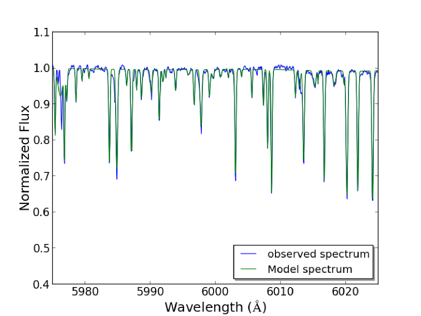
Figure 1: This figure plots a sample of HD 172051 spectrum (black) overploted with the ROBOSPECT model spectrum (green).

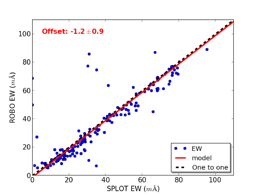
Figure 2: This figure plots the EW of HD 172051 measured two different ways. The first with ROBOSPECT (ROBO), the automated line fitting program, and EW measured with SPLOT in IRAF. Note that ROBOSPECT EW values greater than 100 and less than 5 $m$ Å were removed from the sample.

Through an iterative process, we found that we could achieve qualitative agreement to the observed spectrum by using a window size of 40 mÅ for the local continuum normalization, used 3$\sigma$ to identify the lines and a gaussian profile to measure the EW values. In addition to a visual inspection of the synthetic spectrum produced by ROBOSPECT compared to the observed spectrum (Figure 1), we also compared the ROBOSPECT produced EWs versus EWs tabulated by hand through the use of splot in IRAF. As shown in Figure 2, the EWs determined in an automated fashion via ROBOSPECT mirror those computed by hand. Note that ROBOSPECT tabulated EWs are available as electronic tables in the online version of this manuscript. We do find a statistically insignificant offset in the EWs determined via these two methods (y intercept offset of -1.2 $\pm$ 0.9 $m$Å in Figure 2); however, since this offset appears across all of our calibration sources it suggests the offset might be systematic and not random noise. As we discuss in Section 4.1, this could lead to an underestimation of $[Fe/H]$.

3.2 Determining Fundamental Atmospheric Parameters

We used the well established FORTRAN based program TGVIT (Takeda et al., 2002a, 2005) to calculate the fundamental atmospheric parameters ($T_{eff}$, $log(g)$, $[Fe/H]$) and $v_{t}$for our sample. As described in Takeda et al. (2002a), TGVIT utilizes a tabulated grid of model EWs for Fe I and Fe II lines spanning a range of each of the above fundamental atmospheric parameters and $v_{t}$. The code uses a downhill simplex methodology with the tabulated model EWs to iterate to a final set of fundamental stellar parameters for a spectrum. TGVIT is thus different than SME and MOOG based approaches, which calculate the fundamental atmospheric parameters for every combination of line strength in a given spectrum. TGVIT adopts three criteria that are motivated by the effects of the excitation equilibrium, ionization equilibrium, and microturbulence on Fe I and Fe II EWs:

1 - Fe I abundances should not have dependence on the lower excitation potential.

2 - The abundance derived from Fe I should be equal to the abundance derived from Fe II.

3 - The abundances calculated from individual Fe I and Fe II lines in a given star should not have any dependence on the EW.

As described in detail in Takeda et al. (2002a), these three conditions can be represented by a single dispersion equation (Equation 1).

$$D^{2}\equiv\sigma^{2}_{1}+\sigma^{2}_{2}+(\left<A_{1}\right>-\left<A_{2}\right>)^{2}$$ (1)

Condition 2 can be satisfied where the mean abundance of Fe I ($\left<A_{1}\right>$) must equal the mean abundance of Fe II ($\left<A_{2}\right>$) thus $\left<A_{1}\right>-\left<A_{2}\right>=0$. Conditions 1 and 3 can be satisfied in the same way, where the deviation of the mean abundance of $\left<A_{1}\right>$ ($\sigma_{1}$) and $\left<A_{2}\right>$ ($\sigma_{2}$) must be minimized. Finally, we follow Takeda et al. (2005) and restrict our analysis to Fe I and Fe II lines whose EW’s are less than 100 $m$Å.

Our initial implementation of TGVIT suggested that the best solution could be biased by a few Fe I and Fe II lines that exhibited anomalously high or low EWs. To mitigate this effect, we implemented a bootstrap method similar to that used by McCarthy & Wilhelm (2014). Our method created 150 unique sets of EWs, each of which were comprised of 90% of the original Fe I and Fe II lines measured by ROBOSPECT. We found that our choice of initial fundamental parameters did not affect the results, thus we reused the same initial parameter values ($T_{eff}$= 5000, $log(g)$= 4.0, $v_{t}$= 1.0, $[Fe/H]$= 0.0) for our full sample.

We ran each of the 150 unique sets of EWs through TGIVT. Each TGVIT run computed the best fit parameters, calculated the EW residuals (EW_data- EW_TGVIT), and identified lines that were $\geq$ $2.5\sigma$ outliers. Next, we removed the $\geq$ $2.5\sigma$ outlier lines from the input line list. We then re-ran TGVIT using the initial parameter values. We performed this iterative rejection procedure for a total of 5 times per unique set of EWs. Typically, between 5-20 lines per unique set were removed via this process. Each unique set of EWs provided a single solution of best fit parameter values. We used the mean of the 150 unique sets to compute the final solution of fundamental stellar parameter values for each star.

We computed uncertainties in our fundamental stellar parameters in two steps. First, we adopted the statistical uncertainty calculations within TGVIT described in Takeda et al. (2002a). The algorithm took steps away from the converged solution in one parameter at a time until one of the three conditions noted above, and re-expressed in equations 2, 3, and 4, was violated.

$$|(\chi_{max}-\chi_{min})\times b|<\sigma_{1}$$ (2)

$$|(EW_{max}-EW_{min})\times q|<\sigma_{1}$$ (3)

$$|\left<A_{1}\right>-\left<A_{2}\right>|<e_{1}+e_{2}$$ (4)

In the series of inequalities above, the constants $b$ and $q$ represent the slope of a linear-regression fit of the abundance ($A_{1}$) versus $\chi$ and $A_{1}$ versus EW respectively and the constants $e_{1}$ and $e_{2}$ are the probable error of the abundance ($\sigma/\sqrt[]{N}$), where N is the number of lines used to calculate the abundance. The minimum and maximum values for EW and $\chi$ are taken from the line list and the best fit parameter solution. To compute the uncertainty of a parameter, one of the three parameters ($T_{eff}$, $log(g)$, $v_{t}$) is increased until one of the three above inequalities (Equations 2, 3, 4) is violated. The same parameter is then decreased until it violates one of the three above inequalities (Equations 2, 3, 4). The average of the positive and negative differences of the parameter from the best fit value then defines the uncertainty in that parameter. This process is then repeated for the other two parameters. The final uncertainty in the $[Fe/H]$ abundance was computed by adding the uncertainties in abundance derived from using the accepted range of each of the $T_{eff}$, $log(g)$, $v_{t}$ parameters in quadrature. Note that this methodology tested the convergence of isolated parameters. While McCarthy & Wilhelm (2014) demonstrated that the coupled uncertainties between the atmospheric parameters were negligible their analysis was done using spectra of much higher resolution and for only one solar metalicity star. Thus we suggest that the errors we determine should be conservatively viewed as lower limits.

Our use of the bootstrap method allows us to probe how the choice of Fe I and Fe II lines influences the converged solutions. We calculated the standard deviation of each parameter over the 150 iterations. We then added the bootstrap-derived uncertainties to the internally computed TGVIT uncertainties in quadrature. We note that this final error estimation does not take into account any systematical errors.

3.3 Validating with Calibration Stars

The fundamental atmospheric properties of stars derived by TGVIT and its precursor program (Takeda et al., 2002a, 2005) have been robustly compared against a wide variety of techniques to compute atmospheric parameters. As detailed in Takeda et al. (2005), TGVIT has been shown to yield similar parameters as those computed from theoretical evolutionary tracks, calculated from B-V (Allende Prieto & Lambert, 1999), $uvby$ (Alonso et al., 1996; Olsen, 1984), and IR Photometry (Ribas et al., 2003), calculated from the wings of H$\beta$ and Mg I b (Fuhrmann, 1998), and other spectroscopic analysis programs that invoke similar iterative solution approaches outlined in Heiter & Luck (2003) and Santos et al. (2004). Takeda et al. (2005) also compared TGVIT results to a collection of atmospheric parameters for 134 stars compiled from a variety of literature sources by Cayrel de Strobel et al. (2001). The offsets between TGVIT and these literature compilations were determined to be $T_{eff}$= -39 $\pm$ 101 $K$, $log(g)$= 0.00 $\pm$ 0.19, and $[Fe/H]$= -0.05 $\pm$ 0.08 (Takeda et al., 2005). More recently, McCarthy & Wilhelm (2014) found good agreement between the atmospheric parameters they derived from TGVIT to those derived from SME (Valenti & Fischer, 2005), for a sample of 12 stars.

We briefly extend the comparison of TGVIT-derived atmospheric parameters with those derived via other approaches to calibrate our total line list selection procedure and test our usage of ROBOSPECT+TGVIT against published literature. Specifically, we utilized 8 stars that were not part of the SEEDS survey, but observed with the same resolution, SNR, and instrument as used in our survey (ARCES at APO). The first method we used to compute fundamental stellar parameters (referred to as BPG in Wisniewski et al. 2012) used the 2002 version of MOOG (Sneden, 1973), the one-dimensional plane-parallel model atmospheres interpolated from the ODFNEW grid of ATLAS9 (Castelli & Kurucz, 2004), and a line list of $\sim$ 150 Fe I and Fe II lines compiled from the Solar Flux Atlas (Kurucz et al., 1984), Utrecht spectral line compilation (Moore et al., 1966), and the Vienna Atomic Line Database (Kupka et al., 2000, 1999; Ryabchikova et al., 1997; Piskunov et al., 1995). The second method we used to compute these stellar parameters (referred to as IAC in Wisniewski et al. 2012) also used MOOG Sneden (1973), but with an equivalent width line finding program like ROBOSPECT. The third method we used to compute stellar parameters utilized SME (Valenti & Piskunov, 1996; Valenti & Fischer, 2005), following the methodology described in Petigura et al. (2017).

We processed our observations of these 8 stars in the same manner as our SEEDS target data, measuring line strengths via ROBOSPECT and computing fundamental parameters via TGVIT, as summarized in Section 3.2. The fundamental parameters derived via our approach and the three methods described above are plotted in Figure 3 and summarized in Table The Fundamental Stellar Parameters of FGK Stars in the SEEDS Survey.

To assess the differences between the parameters derived via these three approaches, we fit the data in Figure 3 using the algorithm Orthogonal Distance Regression (ODR) (Boggs & Rogers, 1990) in scipy, which takes into account uncertainties in both the x and y directions. The mean differences between TGVIT parameters and those derived by the three alternative approaches is $<2\sigma$, as seen in Figure 3. We do note that there is a clustering of $log(g)$ values, but these still follow a one-to-one relationship within the errors of the parameters. These results help demonstrate that our use of ROBOSPECT and TGVIT reproduce the atmospheric parameters derived via MOOG, using the same input dataset, but with different line lists.

We also used these 8 calibration stars to explore the optimal line identification procedure to use with ROBOSPECT. Optimizing the line identification procedure is important as unidentified lines effect the placement of the continuum, thus influence the final EW output. Note that these additional lines identified outside of the Fe I and Fe II line list from Takeda et al. (2005) are only used internally for continuum placement in ROBOSPECT and are not used for subsequent analysis. As noted in Section 3.1, ROBOSPECT identifies absorption lines in the spectrum either via a user supplied line list or by searching for n$\sigma$ variations from the local continuum. We found that we were unable to reproduce the atmospheric parameters for our 8 calibration stars derived using other codes (Table The Fundamental Stellar Parameters of FGK Stars in the SEEDS Survey) if we provided no line list to ROBOSPECT. We also noted that using a full line list from VALD (Kupka et al., 2000, 1999; Ryabchikova et al., 1997; Piskunov et al., 1995) required ROSOSPECT to use large computational times. Thus, we used the Fe I and II line list from Takeda et al. (2005) and allowed ROBOSPECT to automatically additional identify lines by looking for 3 $\sigma$ deviations from the continuum.

3.4 Chromospheric Activity Ages

We computed a measure of chromospheric activity of our sample to help constrain their ages. We utilized the chromospheric activity-age relationship from Mamajek & Hillenbrand (2008), shown in equation 5, where $\tau$ is the age of the star in Gyr and $R^{\prime}_{HK}$  is the chromospheric activity index. This relationship is based on chromospheric activity levels measured in young stars in clusters, as well as ages for these clusters derived from isochronal fitting. Thus to calculate the ages of our sample stars, we compute the calcium H and K emission line fluxes (3968.47 Å and 3933.66 Å respectively) from our echelle spectra to determine $R^{\prime}_{HK}$.

$$\log{(\tau)}=-38.053-17.912\log{(R^{\prime}_{HK})}\\ -1.6675\log{(R^{\prime}_{HK})}^{2}$$ (5)

$R^{\prime}_{HK}$  is defined as the luminosity of the Calcium H and K emission lines divided by the total luminosity of the star. We follow Noyes et al. (1984) and compute $R^{\prime}_{HK}$ in Equation 6. Line luminosities, determined by measuring the line emission flux for the H and K lines, are represented by the flux index $S_{HK}$  (Equation 7), where $N_{H}$ and $N_{K}$ are counts from the core of the H and K lines, $N_{V}$ and $N_{R}$ are counts from continuum regions, and $\alpha$ and $\beta$ are correction factors. We use literature values of each star’s $B-V$ magnitude (see Table 4) to represent the continuum contributing to the luminosity of the H and K lines, which is encapsulated in the polynomials $C_{1}$ (Equation 8; see Noyes et al. 1984). The polynomial $C_{2}$ in Equation 9, adopted from Noyes et al. (1984), encapsulates the total luminosity of the star.

$$\log_{10}{(R^{\prime}_{HK})}=\log_{10}{(1.34\times 10^{-4}S_{HK}10^{C_{1}}-10^{C_{2}})}$$ (6)

$$S_{HK}=\alpha\frac{N_{H}+N_{K}}{N_{V}+N_{R}}+\beta$$ (7)

$$C_{1}=1.13\times(B-V)^{3}-3.91\times(B-V)^{2}\\ +2.84\times(B-V)-0.47$$ (8)

$$C_{2}=-4.898+1.918\times(B-V)^{2}-2.893\times(B-V)^{3}$$ (9)

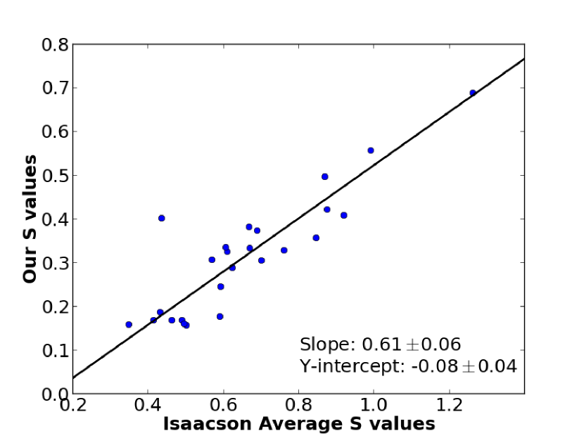
Figure 4: $S_{HK}$indices are plotted for Isaacson & Fischer (2010) and our measured $S_{HK}$values. The $S_{HK}$indicies are calculated from measured H and K Ca lines fluxes. The S values from Isaacson & Fischer (2010) are an average of multiple observations of the same object to study jitter, which affects the value of $S_{HK}$that is calculated. We note that our observations have no control for jitter.

We measured the strength of the calcium H and K emission lines in a 1 Åwide band at the line core, following Middelkoop (1982). We used regions 20 Å-wide centered at 3891 Å and 4001 Å  which are outside of the H and K absorption lines, to measure the local continuum. $N_{V}$ and $N_{R}$ are the average of these continuum locations (3891 Å and 4001 Å respectively). To compute the normalization ($\alpha$) and the offset ($\beta$) factors, we calibrated our $S_{HK}$ index (initially with $\alpha$=1 and $\beta$=0) to $S_{HK}$ index values calculated by Isaacson & Fischer (2010) for 25 stars in common. Figure 4 compares our measured S_HK index to the average S_HK index from Isaacson & Fischer (2010); the linear relation determined via use of the ODR fitting algorithm described in subsection 3.3 yielded these normalization and offset factors. Using the correction factor, we calculated the final $S_{HK}$ index values, the corresponding $R^{\prime}_{HK}$  values, and the resultant ages (see Table 4). Note that Equation 5 from Mamajek & Hillenbrand (2008) is only valid for $\log_{10}{(R^{\prime}_{HK})}$ values between -4.0 and -5.1. The uncertainties quoted in the chromospheric-activity ages in Table 4 are propagated from the uncertainties in the normalization and offset factors ($\alpha$ and $\beta$).

4 Results

We now derive the fundamental atmospheric parameters, chromospheric activity, and age estimates for our entire sample, outlined in Section 3. Our results for the fundamental atmospheric parameters are described in Section 4.1. Finally, we estimate the age of our stars by measuring their chromospheric activity in Section 4.2.

4.1 Atmospheric Parameter Results

We present our atmospheric parameter results using TGVIT in Table 6. We extracted fundamental parameters for 93 stars that had SNR $\geq 50$, were non-double-lined spectroscopic binaries, and were well within the $T_{eff}$  parameter grid of TGVIT. 17 stars could not have their atmospheric parameters robustly determined because they were spectroscopic binaries (3 sources), they could not have their line strengths measured with ROBOSPECT (5 sources), they had too low SNR (4 sources), or TGVIT could not converge on a unique solution (5 sources). We noticed that ROBOSPECT failed to fit the continuum between 4478 to $\sim$ 5500 Å for a subset of early K-type stars. Correspondingly, when data from this spectral range was included in our analysis, the resulting atmospheric parameters derived from TGVIT did not match previously published literature results. We therefore utilized a spectral window of 5500 - 6968 Å for all early K-type stars and used the full spectral window (4478 - 6968 Å) for F and G-type stars. We searched for evidence that this reduced spectral bandpass biased the stellar parameters by looking at the dispersion of our results as a function of the number of Fe II lines used, versus those published by Takeda et al. (2002b, 2005), which also utilizes TGVIT, for the 20 stars common to both surveys, and by Valenti & Fischer (2005), which uses SME for the 49 stars common to both surveys. We identified no differences in the dispersion present, above the $3\sigma$ level, between sources whose parameters were derived from our full spectral windows versus those derived from reduced spectral windows.

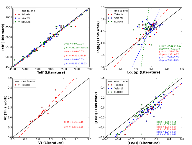
Figure 5: The four above panels compare the four fundamental parameters calculated in this work to those calculated in the Takeda et al. (2005, 2007) which has 19 stars in common with our sample (red circles), (Valenti & Fischer, 2005) which has 52 stars in common with our sample (blue circles), and ELODIE (Prugniel et al., 2007) which has 27 stars in common with our sample (green circles). The solid black line represents a one-to-one relation between our values and literature values. The coloured dashed lines represent a linear fit to the corresponding literature values, with the parameters of the best fit shown in coloured text. $T_{eff}$, $v_{t}$, and $[Fe/H]$show linear relations with previous literature values, and $T_{eff}$and $v_{t}$have values consistent with the one-to-one relation. While error bars are not included in this figure due to clarity, Figure 7 shows the distribution of errors for all four of the atmospheric parameters.

It is common to find systematic offsets in the fundamental atmospheric parameters of stars derived via different methodologies (see e.g. Takeda et al. 2002b; Valenti & Fischer 2005; Prugniel et al. 2007). We explore the level of these potential offsets in our results, to better enable our results to be utilized by future surveys. We compared the amplitude of our fundamental atmospheric parameters to those derived via other spectroscopic methods (Takeda et al., 2002b, 2005; Valenti & Fischer, 2005; Prugniel et al., 2007), for an overlapping subset of stars, and fit a linear relation between them using ODR, as shown in Figure 5. We find that our values of $T_{eff}$ are well matched to these previous studies. We find our values of $v_{t}$  are within $3\sigma$ of Takeda et al. (2002b; 2005), which is the only spectroscopic survey of this group that reports the same flavor of $v_{t}$ as our work. Similarly, although there is dispersion between the $log(g)$ values we derive and those in the literature, these differences are within $3\sigma$ of the errors (Figure 7).

Our derived $[Fe/H]$ values exhibit minor offsets along the y-axis shown in Figure 5. Specifically, our $[Fe/H]$ values are -0.12 $\pm$0.01 dex smaller than Takeda et al. (2002b, 2005), -0.14 $\pm$0.01 dex smaller than Valenti & Fischer (2005), and -0.07 $\pm$ 0.02 smaller than Prugniel et al. (2007). The slope of the $[Fe/H]$ offsets is within $2\sigma$ of unity (see Figure 5), indicating that the offsets are a simple constant that could be used to allow one to place our results on the same absolute scale as each of these literature works. One possible cause of the systematic offset of $[Fe/H]$ is that ROBOSPECT marginally underestimates EWs as compared to measuring line strengths by-hand, as noted in Section 3. To further explore this, we increased the EW values of 4 stars by 1 mÅ re-ran them through TGVIT, and found an average change in $[Fe/H]$ of 0.05. Thus, the marginal underestimation of line strengths by ROBOSPECT can only partially explain these observed offsets.

Finally, to further explore the magnitude and origin of any systematic offsets, we compare the fundamental stellar parameters we computed for our 8 comparison stars (see Figure 3) to the parameters calculated by Takeda et al. (2002b, 2005), Valenti & Fischer (2005), and Prugniel et al. (2007) (see Figure 5). We find that the slopes and intercepts from the 8 sample stars are within $3\sigma$ of the slopes and intercepts from our sample of stars in common with Takeda et al. (2002b, 2005) Valenti & Fischer (2005), and Prugniel et al. (2007) for the $T_{eff}$, $log(g)$, and $v_{t}$ parameters. The $[Fe/H]$ slopes are also within $3\sigma$ of one another; however, the y-intercept offsets computed for the sample of stars in common with Takeda et al. (2002b, 2005) and Valenti & Fischer (2005) are $>3\sigma$ different compared to that from the 8 comparison stars.

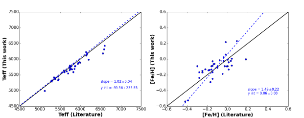
Figure 6: Two panels compare the two fundamental parameters calculated in this work to the photometric Copenhagen-Geneva survey (Casagrande et al., 2011) which has 39 stars in common with our sample. The solid black line represents a one-to-one relation between our values and literature values. The coloured dashed lines represent a linear fit to the corresponding literature values, with the parameters of the best fit shown in coloured text.

For completeness, we also compared the amplitude of our fundamental atmospheric parameters to those derived via photometric methods in the Geneva-Copenhagen survey of Casagrande et al. (2011), as shown in Figure 6. The offset between our results and those from the Geneva-Copenhagen survey is within $3\sigma$ ($0.06\pm 0.03$ dex), for common sources.

Next, we discuss our atmospheric results for GJ 504, a G-type star with a directly imaged low-mass companion (Kuzuhara et al., 2013). The age of this system, and hence the inferred mass of its wide companion, is a subject of debate in the literature. Kuzuhara et al. (2013) considered a wide range of techniques to assess the age of the system, including gyrochronology, chromospheric activity, x-ray activity, lithium abundances, and isochrones, and adopted a most likely age of $160^{+350}_{-60}$ Myrs. Fuhrmann & Chini (2015) and D’Orazi et al. (2016) have revisited the age estimates for GJ 504, and suggested the system has a much older age, thereby increasing the inferred mass of the wide companion into the brown dwarf regime. Both Fuhrmann & Chini (2015) and D’Orazi et al. (2016) suggest that GJ 504 might have recently engulfed a planetary companion, leading to the unusual rotation and Li abundances observed. Recent atmospheric modeling by Skemer et al. (2016) is more consistent with a lower-mass interpretation for the wide companion, hence a younger age estimate for the system, although this work does not exclude the older age hypothesis. The fundamental stellar parameters that we compute for GJ 504, $T_{eff}$  6063 $\pm$ 62, $log(g)$  $4.38\pm 0.13$, and [Fe/H] $0.07\pm 0.05$ are within the range of stellar parameters for system published by Valenti & Fischer (2005), Takeda et al. (2007), da Silva et al. (2012), Ramírez et al. (2013), Fuhrmann & Chini (2015), and D’Orazi et al. (2016). The range of stellar parameters for GJ 504 in some cases exceeds the formal errors quoted for these parameters, likely owing to unrealized calibration offsets between different analysis techniques. We therefore suggest one needs to consider the range of determined fundamental stellar parameters for the system when using these data to determine an age via isochrones.

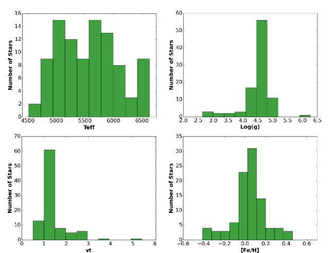
Figure 8: Histograms of the four atmospheric parameters determined for stars in our sample using TGVIT (Table 6); $T_{eff}$ (upper left), $log(g)$ (upper right), $v_{t}$ (lower left), and $[Fe/H]$ (lower right).

The distribution of our atmospheric parameters for our full sample of stars listed is compiled in Table 6. Figure 8 shows histograms of our atmospheric parameters: $T_{eff}$, $log(g)$, $v_{t}$, and $[Fe/H]$. The $T_{eff}$ distribution exhibits a fairly uniform distribution across FGK space, whereas $v_{t}$ and $log(g)$ exhibit peaks that are consistent with main sequence stars. Finally, the $[Fe/H]$ distribution of our sample exhibits a roughly gaussian profile around $0.0~{}dex$, consistent with stars in the solar neighborhood (Casagrande et al., 2011).

4.2 Chromospheric Activity and Ages

We present the chromospheric activity index and associated age estimations for our sample in Table 4. 80 of the 112 stars in our sample had sufficiently strong Ca II H and K emission lines and $B-V$ Values within the validity range of Eq. 5.

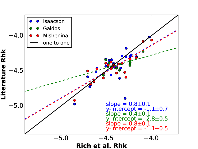
Figure 9: This figure compares the previously published literature results of chromospheric activity ($R^{\prime}_{HK}$) from Isaacson & Fischer (2010) (blue), Gaidos et al. (2000) (green), and (Mishenina et al., 2012) (red) to our calculated $R^{\prime}_{HK}$values (Table 4). The black line is a one-to-one match and the dashed coloured lines are the best linear fit lines using ODR. Results of the fit are printed in coloured text on the bottom right of the figure.

to allow us to calculate $R^{\prime}_{HK}$ values. Our results are consistent with those tabulated by Isaacson & Fischer (2010), Gaidos et al. (2000), and Mishenina et al. (2012) (Figure 9). We note that differences from previous published values can result from adopting different $B-V$ values used when calculating $R^{\prime}_{HK}$ and/or intrinsic variability in the level of a star’s chromospheric activity (see e.g. Isaacson & Fischer 2010). We determined ages for 51 stars with $R^{\prime}_{HK}$ values within limits of the chromospheric activity-age relation (Mamajek & Hillenbrand, 2008) as shown in Table 4.

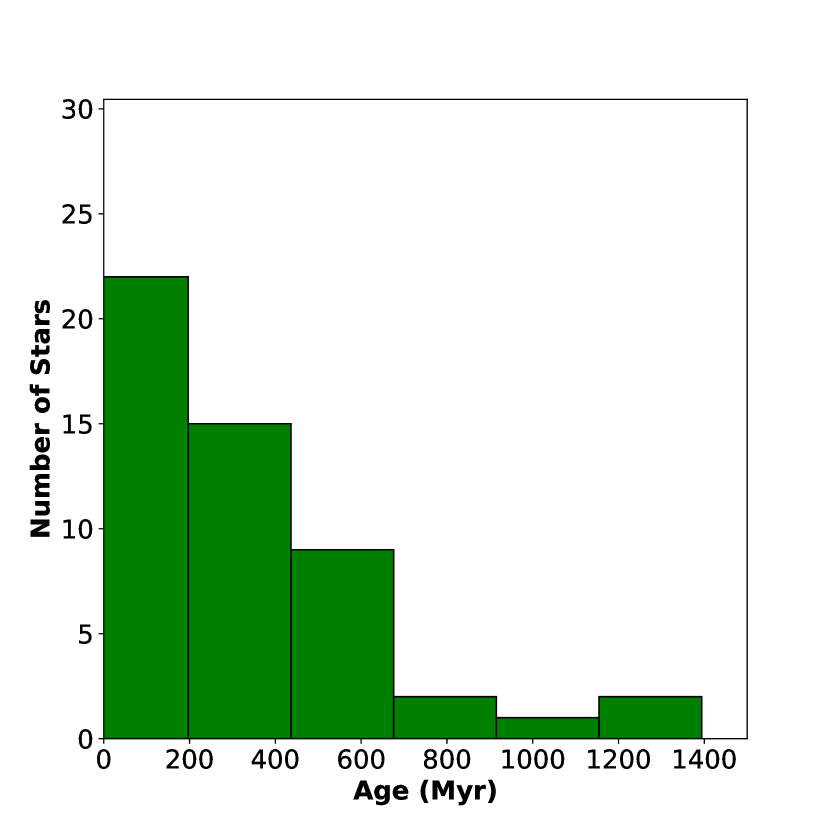
Figure 10: Histogram of the calculated ages (Table 4) using the chromospheric activity index.

Figure 10 shows the sample of SEEDS stars for which we were able to derive ages; the majority of the ages are $<500Myr$. Note that this distribution is not indicative of the complete age distribution of the SEEDS survey, as targets were not selected based on their age. Older stars ($>$ 1.5 Gyr) are outside of the chromospheric activity-age relation, and thus do not have accurate age estimates (Mamajek & Hillenbrand, 2008).

It is important to note that while many stars in the SEEDS sample have ages $<500Myr$, their determined ages are still too old to distinguish between core accretion (Pollack et al., 1996) or disk instability (Boss, 2001) formation scenarios. Planets formed via core accretion are thought to loose most of their heat through the accretion process resulting in "cold-start" planets (Spiegel & Burrows, 2012), while planets formed via disk instability retain a lot of their initial heat resulting in "hot-start" planets (Spiegel & Burrows, 2012). One can distinguish "cold-start" from "hot-start" directly imaged planets via their thermal emission up to an age of $\sim 100Myr$ old. While 6 of our stars have ages $<100Myr$ (see Table 4), the rest of our sample have ages that are either too old or inaccurate to distinguish between cold-start and hot-start formation scenarios for any giant planets they contain Spiegel & Burrows (2012).

We compare our computed chromospheric ages for stars in known moving groups against the accepted ages for these moving groups. Mamajek & Hillenbrand (2008) notes a dispersion for moving group members of 0.25 dex for stars older than 100 Myr and 1 dex for stars less than 100 Myr. The chromospheric age we determine for the one star in our sample (HD 17925; 42 $\pm$ 12 Myr) in $\beta$ Pic Moving Group is consistent within $2\sigma$ with the estimated cluster age of 23 $\pm$ 3 Myr (Mamajek & Bell, 2014). Similarly, the ages for the three stars in our sample that are part of the Local Association Moving Group, HD 166 (78 $\pm$ 28 Myr), HD 37394 (411 $\pm$ 142 Myr), and HD 206860 (340 $\pm$ 201 Myr), are within $2\sigma$ of the moving group age of 20-150 Myr (Gálvez-Ortiz et al., 2010). The age of our single star located in the Hyades moving group, V401 Hya (205 $\pm$ 95 Myr) is marginally within the 3$\sigma$ range of the moving groups age of 50 $\pm$ 100 Myr (Brandt & Huang, 2015). The largest dispersion in ages for our stars within moving groups was found in objects located with the Ursa Major moving group. Although age estimates of this group range from 200-600 Myr (Eiff et al. 2016 and references therein), analysis using MESA models have led to a more recent, precise age of $414\pm 23$ Myr (Jones et al., 2015). Our ages for HD 43989 (112 $\pm$ 58 Myr), HD 63433 (622 $\pm$ 328 Myr), HD 72985 (79 $\pm$ 36 Myr), and HD 135599 (29 $\pm$ 40 Myr) are generally younger than the accepted age of the moving group, although including the 0.25 dex dispersion in the Mamajek & Hillenbrand (2008) chromospheric age relationship brings all of these age estimates within 3-$\sigma$ agreement except for HD 135599.

Finally, we note that our chromospheric age estimate from our single observation of GJ 504 ($618\pm 390$ Myr) is consistent with, albeit less precise than, the previously published chromospheric age ($330\pm 180$ Myr; Kuzuhara et al. 2013). We attribute our lower precision to the fact that our age is based on a single epoch of chromospheric activity, whereas the previous chromospheric activity age calculation is based on 30 years of observations.

5 Conclusion

We have presented the fundamental atmospheric parameters ($T_{eff}$, $log(g)$, $[Fe/H]$), $v_{t}$, chromospheric activity, and age determinations of a subset the FGK stars in the SEEDS survey, based on analysis of high quality, high resolution spectroscopic observations. We demonstrated the reliability of our methodology by comparing a subset of our results to those published in the literature. To aid future comparison of our stellar parameter results with those derived using alternate methodologies, we compile offsets for our computed $[Fe/H]$ values, (0.06, -0.07, -0.12, -0.14 dex), compared to the respective literature sources (Casagrande et al. 2011, Prugniel et al. 2007, Takeda et al. 2002b; 2005, and Valenti & Fischer 2005). Finally, we compared our chromospheric activity and age determinations to previous sources (Isaacson & Fischer 2010, Gaidos et al. 2000, and Mishenina et al. 2012), and to ages of stars associated with moving groups with known ages. Our results will aid the interpretation of the frequency of wide stellar and sub-stellar mass companions detected via the SEEDS survey, and comparison of the results of the SEEDS survey with other high-contrast planet and sub-stellar mass imaging surveys.

6 Acknowledgements

We thank our referee, Ulrike Heiter, for providing constructive feedback that improved the content and clarity of this manuscript. This work has made use of the VALD database, operated at Uppsala University, the Institute of Astronomy RAS in Moscow, and the University of Vienna. This research made use of Astropy, a community-developed core Python package for Astronomy (Astropy Collaboration et al., 2013). This research has made use of the VizieR catalogue access tool, CDS, Strasbourg, France. The original description of the VizieR service was published in A&AS 143, 23.

¹Homer L. Dodge Department of Physics, University of Oklahoma, Norman, OK 73071, USA; erich66210@ou.edu, wisniewski@ou.edu
²Exoplanets and Stellar Astrophysics Laboratory, Code 667, Goddard Space Flight Center, Greenbelt, MD 20771, USA
³Astrobiology Center of NINS, 2-21-1 Osawa, Mitaka, Tokyo, 181-8588, Japan
⁴National Astronomical Observatory of Japan, 2-21-1, Osawa, Mitaka, Tokyo, 181-8588, Japan
⁵Subaru Telescope, National Astronomical Observatory of Japan, 650 North A’ohoku Place, Hilo, HI 96720, USA
⁶Institute of Astrophysics and Planetary Sciences, Faculty of Science, Ibaraki University, 2-1-1 Bunkyo, Mito, Ibaraki 310-8512, Japan
⁷Laboratoire Lagrange (UMR 7293), Universite de Nice-Sophia Antipolis, CNRS, Observatoire de la Cote d’Azur,
  28 avenue Valrose, F-06108 Nice Cedex 2, France
⁸Max Planck Institute for Astronomy, Königstuhl 17, D-69117 Heidelberg, Germany
⁹Astrophysics Department, Institute for Advanced Study, Princeton, NJ 08540, USA
¹⁰Harvard-Smithsonian Center for Astrophysics, 60 Garden Street, Cambridge, MA 02138, USA ¹¹Department of Physics and Astronomy, College of Charleston, 58 Coming St., Charleston, SC 29424, USA
¹²Graduate School of Science, Osaka University, 1-1 Machikaneyama, Toyonaka, Osaka 560-0043, Japan
¹³Exoplanets and Stellar Astrophysics Laboratory, Code 667, Goddard Space Flight Center, Greenbelt, MD 20771, USA
¹⁴Eureka Scientific, 2452 Delmer, Suite 100, Oakland CA 96002, USA
¹⁵Goddard Center for Astrobiology
¹⁶Department of Physics, Hobart and William Smith Colleges, Geneva, NY 14456, USA
¹⁷Department of Astrophysics, Nicolaus Copernicus Astronomical Center, ul. Rabiańska 8, PL-87-100 Toruń, Poland
¹⁸Institute for Astronomy, University of Hawaii, 640 N. A’ohoku Place, Hilo, HI 96720, USA
¹⁹Department of Astronomy, Stockholm University, AlbaNova University Center, SE-10691 Stockholm, Sweden
²⁰Department of Astrophysical Science, Princeton University, Peyton Hall, Ivy Lane, Princeton, NJ 08544, USA
²¹Department of Earth and Planetary Sciences, Tokyo Institute of Technology, 2-12-1 Ookayama, Meguro-ku, Tokyo 152-8551, Japan
²²Department of Astronomy, The University of Tokyo, 7-3-1, Hongo, Bunkyo-ku, Tokyo, 113-0033, Japan
²³Department of Astronomy, Kyoto University, Kitashirakawa-Oiwake-cho, Sakyo-ku, Kyoto 606-8502, Japan
²⁴The Center for the Promotion of Integrated Sciences, The Graduate University for Advanced Studies (SOKENDAI),
  Shonan International Village, Hayama-cho, Miura-gun, Kanagawa 240-0193, Japan
²⁵Hiroshima University, 1-3-2, Kagamiyama, Higashi-Hiroshima 739-8511, Japan
²⁶College of Science, Ibaraki University, Bunkyo 2-1-1, Mito, 310-8512 Ibaraki, Japan
²⁷Space Telescope Science Institute, 3700 San Martin Dr., Baltimore, MD 21218, USA
²⁸Center for Astrophysical Sciences, Johns Hopkins University, Baltimore, MD 21218, USA
²⁹Department of Space Astronomy and Astrophysics Institute of Space & Astronautical Science (ISAS)
  Japan Aerospace Exploration Agency (JAXA) 3-1-1 Yoshinodai, Chuo-ku, Sagamihara, Kanagawa 252-5210, Japan
³⁰National Meteorological Satellite Center, 64-18 Guam-gil, Gawnghyewon-myeon, Jincheon-gun, Chungcheongbuk-do, 27803, Republic of Korea
³¹NExScI, California Institute of Technology, Pasadena, CA, 91109, USA
³²Jet Propulsion Laboratory, California Institute of Technology, Pasadena, CA, 91109, USA
³³Department of Physics, University of Cincinnati, Cincinnati, OH 45221, USA
³⁴Space Science Institute, 475 Walnut Street, Suite 205, Boulder, CO 80301, USA
³⁵Department of Astronomical Science, The Graduate University for Advanced Studies, 2-21-1, Osawa, Mitaka, Tokyo, 181-8588, Japan
³⁶Institute of Astronomy and Astrophysics, Academia Sinica, P.O. Box 23-141, Taipei 10617, Taiwan
³⁷Institute for Astronomy, ETH Zurich, Wolfgang-Pauli-Strasse 27, 8093 Zurich, Switzerland
³⁸Department of Cosmosciences, Hokkaido University, Kita-ku, Sapporo, Hokkaido 060-0810, Japan
³⁹Astronomical Institute, Tohoku University, Aoba-ku, Sendai, Miyagi 980-8578, Japan

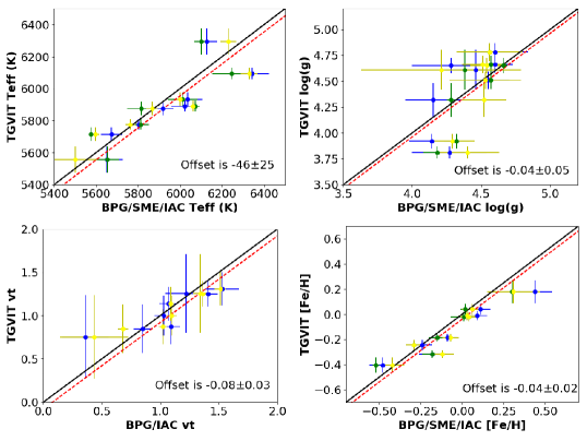
Figure 3: Plots the stellar parameters of the 8 calibration stars listed in Table The Fundamental Stellar Parameters of FGK Stars in the SEEDS Survey compared to this work’s stellar parameters. The three methods utilized are colour coated where SME is blue, ARES is yellow, and BPG is green. Each subplot represents a different stellar parameter plotting the one to one line, and the best-fitting line with each y-axis offset labeled in the subfigure.

Figure 7: Demonstrate the difference between literature values for fundamental stellar parameters and those computed via this manuscript are presented as a function of the uncertainties in these parameters. Takeda et al. (2005, 2007) are the red circles, which has 19 stars in common with our sample. (Valenti & Fischer, 2005) are the blue circles, which has 52 stars in common with our sample. The dashed black lines represent $3\sigma$, thus anything to the right of the dashed lines is within $3\sigma$.

Table 1: Basic information for our targets. A full observational list of all F,G, and K stars observed within the SEEDs sample. (1) Gaidos et al. (2000), (2) ESA (1997), (3) Brandt et al. (2014), (4) Houk & Smith-Moore (1988), (5) Stephenson (1986), (6) Torres et al. (2006), (7) Ehrenreich & Désert (2011), (8) Faedi et al. (2013), (9) Bergfors et al. (2013).

HD	HIP	Other	RA	Dec	Date Obs.	moving	SNR at	Spectral
		Name				group	6000 Å	Classification
166	544	V439 And	0:06:37	29:01:17	2011-03-20	Local Association(1)	199.5	K0V(2)
984	1134	BD-08 2400	0:14:10	-7:11:57	2010-10-17	…	250	F5(2)
1835	1803	BE Cet	0:22:52	-12:12:34	2012-11-28	…	292	G3V(2)
4128	3419	$\beta$ Cet	0:43:35	-17:59:12	2012-10-24	…	310	K0III(2)
4277	3589	BD+54 144	0:45:51	54:58:40	2012-12-09	…	70	F8V(2)
4747	3850	GJ 36	0:49:27	-23:12:45	2010-10-16	…	397	G8/K0V(2)
4813	3909	19 Cet	0:50:08	-10:38:40	2011-03-17	…	230	F7IV-V(2)
5608	4552	HR 275	0:58:14	33:57:03	2012-10-29	…	271	K0(2)
7590	5944	V445 And	1:16:29	42:56:22	2012-12-30	…	251	G0(2)
7661	5938	EW Cet	1:16:24	-12:05:49	2012-12-27	…	360	K0V(2)
8673	6702	LTT 10515	1:26:09	34:34:47	2012-12-05	…	330	F7V(2)
8907	6878	BD+41 283	1:28:34	42:16:04	2011-03-17	…	232	F8(2)
8941	6869	BD+16 154	1:28:24	17:04:45	2012-12-30	…	483	F8IV-V(2)
9826	7513	$\upsilon$ And	1:36:48	41:24:20	2012-12-05	…	345	F8V(2)
10700	8102	$\tau$ Cet	1:44:04	-15:56:15	2012-12-27	…	350	G8V(2)
10780	8362	V987 Cas	1:47:45	63:51:09	2012-10-04	…	352	K0V(2)
11636	8903	$\beta$ Ari	1:54:38	20:48:28	2012-12-22	…	289	A5V…(2)
12039	9141	DK Cet	1:57:49	-21:54:05	2012-12-30	Tuc-Hor(3)	133	G3/G5V(2)
13507	10321	V450 And	2:12:55	40:40:06	2012-12-05	…	225	G0(2)
13594	10403	HR 647	2:14:03	47:29:03	2012-12-27	…	287	F5V(2)
14067	10657	HR 665	2:17:10	23:46:04	2012-12-05	…	257	G9III(2)
14082B	10679	BD+28 382B	2:17:25	28:44:42	2012-12-09	…	272	G2V(2)
16160	12114	HR 753	2:36:05	6:53:13	2012-12-30	…	296	K3V(2)
16760	12638	BD+37 604	2:42:21	38:37:07	2012-12-09	…	255	G5(2)
17250	12925	BD+04 439	2:46:15	5:35:33	2012-11-28	…	168	F8(2)
17925	13402	EP Eri	2:52:32	-12:46:11	2010-11-19	beta Pic(3)	281	K1V(2)
18632	13976	BZ Cet	3:00:03	7:44:59	2012-12-27	…	218	G5(2)
20630	15457	$\kappa$ Cet	3:19:22	3:22:13	2012-11-26	…	297	G5Vvar(2)
22781	17187	BD+31 630	3:40:50	31:49:35	2012-11-26	…	281	K0(2)
24916	18512	BD-01 565	3:57:29	-1:09:34	2012-11-26	…	260	K4V(2)
25457	18859	BD-00 423	4:02:37	-0:16:08	2010-10-02	…	377	F5V(2)
25665	19422	BD+69 238	4:09:35	69:32:29	2010-10-17	…	247	G5(2)
25998	19335	V582 Per	4:08:37	38:02:23	2012-11-26	…	270	F7V(2)
29697	21818	V834 Tau	4:41:19	20:54:05	2010-11-19	…	258	K3V(2)
30495	22263	IX Eri	4:47:36	-16:56:04	2012-11-28	…	294	G3V(2)
31000	22776	V536 Aur	4:53:56	36:45:27	2012-10-24	…	207	G5(2)
35850	25486	AF Lep	5:27:05	-11:54:04	2012-12-27	…	348	F7V(2)
36869	…	AH Lep	5:34:09	-15:17:03	2012-11-26	…	393	G2V(4)
37394	26779	V538 Aur	5:41:20	53:28:52	2011-03-17	Local Association(1)	350	K1V(2)
37484	26453	GC 7011	5:37:40	-28:37:35	2010-11-19	…	267	F3V(2)
38393	27072	LTT 2364	5:44:28	-22:26:54	2010-10-17	…	346	F7V(2)
39587	27913	chi01 Ori	5:54:23	20:16:34	2010-11-19	…	313	G0V(2)
40774	28526	BD+09 1055	6:01:17	9:04:20	2012-10-04	…	190	G5(2)
41593	28954	V1386 Ori	6:06:40	15:32:32	2012-12-27	…	337	K0(2)
43162	29568	GJ 3389	6:13:45	-23:51:43	2012-10-24	…	229	G5V(2)
43989	30030	V1358 Ori	6:19:08	-3:26:20	2012-12-09	Ursa Major(1)	217	G0(2)
59747	36704	DX Lyn	7:33:01	37:01:47	2012-10-24	…	200	G5(2)
60737	37170	GC 10209	7:38:16	47:44:55	2012-12-30	…	180	G0(2)
61606	37349	V869 Mon	7:39:59	-3:35:51	2012-12-27	…	232.3	K2V(2)
63433	38228	V377 Gem	7:49:55	27:21:48	2012-12-27	Ursa Major(1)	294	G5IV(2)
68988	40687	BD+61 1038	8:18:22	61:27:39	2010-10-02	…	192	G0(2)
69830	40693	LHS 245	8:18:24	-12:37:56	2012-12-27	…	223	K0V(2)
72760	42074	BD-00 2024	8:34:32	-0:43:34	2012-12-05	…	275	G5(2)
72905	42438	3 UMa	8:39:12	65:01:15	2012-12-30	Ursa Major(3)	217	G1.5Vb(2)
73350	42333	V401 Hya	8:37:50	-6:48:25	2012-12-30	Hyades(1)	231	G0(2)
75732	43587	LHS 2062	8:52:36	28:19:51	2010-11-19	…	160	G8V(2)
76151	43726	BD-04 2490	8:54:18	-5:26:04	2012-12-30	…	219	G3V(2)
77825	44526	BD-15 2685	9:04:20	-15:54:51	2012-10-24	…	110	K2V(2)
79555	45383	HEI 350	9:14:55	4:26:35	2012-12-05	…	310	K0(2)

Table 2: continued

Basic information for our targets. A full observational list of all F,G, and K stars observed within the SEEDs sample. (1) Gaidos et al. (2000), (2) ESA (1997), (3) Brandt et al. (2014), (4) Houk & Smith-Moore (1988), (5) Stephenson (1986), (6) Torres et al. (2006), (7) Ehrenreich & Désert (2011), (8) Faedi et al. (2013), (9) Bergfors et al. (2013). HD HIP Other RA Dec Date Obs. moving SNR at Spectral Name group 6000 Å Classification 80715 45963 GJ 1124 9:22:26 40:12:04 2012-12-30 … 320 K2V⁽²⁾ 81040 46076 BD+20 2314 9:23:47 20:21:52 2012-10-29 … 286 G0⁽²⁾ 82106 46580 LHS 2147 9:29:55 5:39:19 2012-10-24 … 311 K3V⁽²⁾ 82443 46843 DX Leo 9:32:44 26:59:19 2011-02-14 … 297 K0⁽²⁾ 82558 46816 LQ Hya 9:32:26 -11:11:05 2011-04-17 … 176 K0⁽²⁾ 87424 49366 V417 Hya 10:04:38 -11:43:47 2012-12-05 … 205 K0⁽²⁾ 89744 50786 BD+41 2076 10:22:11 41:13:46 2010-10-16 … 360 F7V⁽²⁾ 90839 51459 GJ 395 10:30:38 55:58:50 2012-12-05 … 321 F8V⁽²⁾ 94765 53486 GY Leo 10:56:31 7:23:19 2012-12-05 … 195 K0⁽²⁾ 95174 … LTT 12936 10:59:38 25:26:16 2012-12-09 … 160 K4V⁽⁵⁾ 96064 54155 HH Leo 11:04:42 -4:13:16 2012-12-09 … 230 G5⁽²⁾ 96167 54195 BD-09 3201 11:05:15 -10:17:29 2012-12-22 … 149 G5⁽²⁾ 97658 54906 BD+26 2184 11:14:33 25:42:37 2010-10-16 … 340 K1V⁽²⁾ 98649 55409 LTT 4199 11:20:52 -23:13:02 2012-12-05 … 147 G3/G5V⁽²⁾ 102956 57820 BD+58 1340 11:51:23 57:38:27 2012-11-28 … 170 K0III⁽²⁾ 105631 59280 BD+41 2276 12:09:37 40:15:07 2011-04-17 … 243 K0V⁽²⁾ 109272 61296 HR 4779 12:33:34 -12:49:49 2012-12-05 … 279 G8III/IV⁽²⁾ 112733 63317 BD+39 2586 12:58:32 38:16:44 2012-12-09 … 173 G5V⁽²⁾ 115383 64792 GJ 504 13:16:47 9:25:27 2011-04-17 … 280 G0Vs⁽²⁾ 115617 64924 61 Vir 13:18:24 -18:18:40 2011-03-20 … 249 G5V⁽²⁾ 120136 67275 $\tau$ Boo 13:47:16 17:27:25 2012-12-22 … 455 F7V⁽²⁾ 120352 67412 BD-00 2743 13:48:58 -1:35:35 2011-03-20 … 337 K0⁽²⁾ 128167 71284 $\sigma$ Boo 14:34:41 29:44:43 2012-12-22 … 279 F3Vwvar⁽²⁾ 128311 71395 HN Boo 14:36:01 9:44:48 2012-12-05 … 242 K0⁽²⁾ 129333 71631 Ek Dra 14:39:00 64:17:30 2011-03-20 … 291 F8⁽²⁾ 134083 73996 45 Boo 15:07:18 24:52:09 2011-03-20 … 480 F5V⁽²⁾ 135599 74702 V379 Ser 15:15:59 0:47:47 2010-10-02 Ursa Major⁽¹⁾ 251 K0⁽²⁾ 145229 79165 BD+11 2925 16:09:27 11:34:28 2012-12-22 … 167 G0⁽²⁾ 152555 82688 BD-04 4194 16:54:08 -4:20:25 2010-10-17 … 334 G0⁽²⁾ 189733 98505 V452 Vul 20:00:44 22:42:39 2012-12-30 … 208 G5⁽²⁾ 199665 103527 18 Del 20:58:26 10:50:21 2012-12-30 … 246 G6III⁽²⁾ 202575 105038 LTT 16242 21:16:33 9:23:38 2011-04-17 … 302 K2⁽²⁾ 206466 107146 BD+08 3000 12:19:07 16:32:54 2010-10-17 … 228 K2⁽²⁾ 206860 107350 HN Peg 21:44:31 14:46:19 2010-10-16 Local Assocation⁽¹⁾ 254 G0V⁽²⁾ 210667 109527 V446 Lac 22:11:12 36:15:23 2012-12-30 … 206 K0⁽²⁾ 212698 … 53 Aqr A 22:26:34 -16:44:32 2012-11-28 … 333 G2V⁽⁶⁾ 213845 111449 NLTT 54210 22:34:42 -20:42:30 2012-12-27 … 247 F7V⁽²⁾ 217343 113579 GC 32053 23:00:19 -26:09:13 2012-12-27 … 231 G3V⁽²⁾ 217813 113829 MT Peg 23:03:05 20:55:07 2012-11-28 … 266 G5V⁽²⁾ 220182 115331 V453 And 23:21:37 44:05:52 2012-10-04 … 215 K1V⁽²⁾ 222582 116906 BD-06 6262 23:41:52 -5:59:09 2012-11-28 … 253 G5⁽²⁾ 283750 21482 V833 Tau 4:36:48 27:07:56 2010-10-02 … 302 K2⁽²⁾ … 36357 V376 Gem 7:29:02 31:59:38 2012-10-24 … 135 K2V⁽²⁾ … 97657 HatP 11 19:50:50 48:04:51 2012-12-27 … 158 K5V⁽²⁾ … 115162 BD+41 4749 23:19:40 42:15:10 2012-12-27 … 260 G0⁽²⁾ … … BD+05 4576 20:39:55 6:20:12 2012-12-27 … 99 K7V⁽⁵⁾ … … HatP 13 8:39:32 47:21:07 2012-10-29 … 160 G4⁽⁷⁾ … … HatP 17 21:38:09 30:29:19 2012-12-30 … 154 … … … HatP 30 8:15:48 5:50:12 2012-11-28 … 136 … … … HatP 6 23:39:06 42:27:58 2012-12-09 … 100 F8V⁽⁸⁾ … … Wasp 12 6:30:33 29:40:20 2012-11-26 … 83 G0V⁽⁹⁾

Table 3: Tabulated comparison of our methods to three alternative methods utilizing 8 calibration stars. These results are plotted in Figure 3. (a) See Petigura et al. (2017) for a description of the methods used to calculate these parameters. (b) See Wisniewski et al. (2012) for a description of the methods used to calculate these parameters. These stars were used to test and calibrate the two stellar characterization pipelines in Wisniewski et al. (2012) and Ghezzi et al. (2014), but their computed fundamental stellar parameters were not formally reported in those publications.

Study Name	Name	$T_{eff}$	$log(g)$	$v_{t}$	$[Fe/H]$	Reference
		(K)	log10($cm/s^{2}$)	($\frac{km}{sec}$)	(dex)
	GSC 01240-00945	6095.2 $\pm$ 34.8	3.81 $\pm$ 0.06	1.309 $\pm$ 0.193	-0.318 $\pm$ 0.030	…
	HD 20630	5776.4 $\pm$ 33.5	4.65 $\pm$ 0.073	1.137 $\pm$ 0.196	-0.011 $\pm$ 0.037	…
	HD 22484	5891.1 $\pm$ 32.1	3.92 $\pm$ 0.07	1.252 $\pm$ 0.147	-0.187 $\pm$ 0.031	…
This Work	HD 153458	5875.9 $\pm$ 42.1	4.66 $\pm$ 0.085	1.001 $\pm$ 0.226	0.042 $\pm$ 0.044	…
	HD 172051	5714.5 $\pm$ 42.9	4.78 $\pm$ 0.089	0.847 $\pm$ 0.280	-0.245 $\pm$ 0.042	…
	HIP 67526	5932.9 $\pm$ 42.2	4.51 $\pm$ 0.086	0.874 $\pm$ 0.201	-0.020 $\pm$ 0.037	…
	TYC 1275-27-1 (MC5)	6294.8 $\pm$ 84.1	4.32 $\pm$ 0.164	1.255 $\pm$ 0.458	-0.405 $\pm$ 0.063	…
	GSC 03546-01452	5556.1 $\pm$ 83.1	4.61 $\pm$ 0.193	0.753 $\pm$ 0.486	0.178 $\pm$ 0.091	…
	GSC 01240-00945	6246 $\pm$ 92	4.18 $\pm$ 0.10	…	-0.18 $\pm$ 0.06	(a)
	HD 20630	5814 $\pm$ 38	4.66 $\pm$ 0.03	…	0.03 $\pm$ 0.02	(a)
	HD 22484	6074 $\pm$ 18	4.32 $\pm$ -0.09	…	-0.15 $\pm$ 0.05	(a)
SME	HD 153458	5816 $\pm$ 68	4.57 $\pm$ 0.11	…	0.02 $\pm$ 0.03	(a)
	HD 172051	5576 $\pm$ 9	4.56 $\pm$ 0.01	…	-0.29 $\pm$ 0.01	(a)
	HIP 67526	6013 $\pm$ 72	4.57 $\pm$ 0.14	…	0.01 $\pm$ 0.08	(a)
	TYC 1275-27-1 (MC5)	6101 $\pm$ 34	4.28 $\pm$ 0.03	…	-0.52 $\pm$ 0.02	(a)
	GSC 03546-01452	5654 $\pm$ 55	4.38 $\pm$ 0.14	…	0.30 $\pm$ 0.05	(a)
	GSC 01240-00945	6330 $\pm$ 40	4.40 $\pm$ 0.23	1.513 $\pm$ 0.05	-0.12 $\pm$ 0.07	Wright et al. 2013
	HD 20630	5764 $\pm$ 22	4.54 $\pm$ 0.12	1.086 $\pm$ 0.029	0.03 $\pm$ 0.05	(b)
	HD 22484	6063 $\pm$ 19	4.29 $\pm$ 0.16	1.361 $\pm$ 0.024	-0.07 $\pm$ 0.05	(b)
IAC	HD 153458	5867 $\pm$ 27	4.51 $\pm$ 0.15	1.096 $\pm$ 0.042	0.06 $\pm$ 0.06	(b)
	HD 172051	5596 $\pm$ 19	4.56 $\pm$ 0.24	0.682 $\pm$ 0.043	-0.29 $\pm$ 0.05	(b)
	HIP 67526	6000 $\pm$ 24	4.53 $\pm$ 0.26	1.021 $\pm$ 0.035	0.04 $\pm$ 0.05	Jiang et al. 2013
	TYC 1275-27-1 (MC5)	6230 $\pm$ 37	4.52 $\pm$ 0.16	1.343 $\pm$ 0.065	-0.42 $\pm$ 0.07	Ghezzi et al. 2014
	GSC 03546-01452	5502 $\pm$ 100	4.21 $\pm$ 0.58	0.433 $\pm$ 0.290	0.31 $\pm$ 0.16	De Lee et al. 2013
	GSC 01240-00945	6344 $\pm$ 81	4.27 $\pm$ 0.27	1.53 $\pm$ 0.14	-0.18 $\pm$ 0.08	Wright et al. 2013
	HD 20630	5803.0 $\pm$ 43.0	4.28 $\pm$ 0.28	1.07 $\pm$ 0.08	0.09 $\pm$ 0.06	(b)
	HD 22484	6023.0 $\pm$ 63.0	4.14 $\pm$ 0.16	1.41 $\pm$ 0.08	-0.09 $\pm$ 0.06	(b)
BPG	HD 153458	5918.0 $\pm$ 50.0	4.60 $\pm$ 0.13	1.03 $\pm$ 0.08	0.11 $\pm$ 0.06	(b)
	HD 172051	5674.0 $\pm$ 50.0	4.60 $\pm$ 0.24	0.85 $\pm$ 0.08	-0.24 $\pm$ 0.06	(b)
	HIP 67526	6037 $\pm$ 71	4.55 $\pm$ 0.15	1.09 $\pm$ 0.08	0.04 $\pm$ 0.06	Jiang et al. 2013
	TYC 1275-27-1 (MC5)	6127.0 $\pm$ 50.0	4.15 $\pm$ 0.2	1.22 $\pm$ 0.18	-0.48 $\pm$ 0.08	Ghezzi et al. 2014
	GSC 03546-1452	5652.0 $\pm$ 75	4.46 $\pm$ 0.16	0.36 $\pm$ 0.20	0.44 $\pm$ 0.10	De Lee et al. 2013

Table 4: Chromospheric Activity Index and Ages

HD	HIP	Other Name	B-V	B-V references	$S_{HK}$	$R^{\prime}_{HK}$	Age (Myr)
166	544	V439 And	0.75	(Zboril & Byrne, 1998)	0.607	-4.23 $\pm$ 0.04	78 $\pm$ 28
984	1134	BD-08 2400	0.5	(Høg et al., 2000)	0.317	-4.36 $\pm$ 0.08	216 $\pm$ 136
1835	1803	BE Cet	0.66	(Ducati, 2002)	0.356	-4.43 $\pm$ 0.07	384 $\pm$ 198
4128	3419	$\beta$ Cet	1.01	(Ducati, 2002)	0.345	-4.79 $\pm$ 0.06	…
4747	3850	GJ 36	0.772	(Koen et al., 2010)	0.277	-4.68 $\pm$ 0.09	…
4813	3909	19 Cet	0.5	(Herbig, 1965)	0.145	-4.96 $\pm$ 0.30	…
5608	4552	HR 275	0.991	(Jofré et al., 2015)	0.278	-4.87 $\pm$ 0.07	…
7590	5944	V445 And	0.58	(Høg et al., 2000)	0.342	-4.38 $\pm$ 0.08	265 $\pm$ 151
7661	5938	EW Cet	0.77	(Høg et al., 2000)	0.566	-4.29 $\pm$ 0.04	124 $\pm$ 45
8673	6702	LTT 10515	0.47	(Masana et al., 2006)	0.155	-4.85 $\pm$ 0.15	…
8907	6878	BD+41 283	0.49	(Høg et al., 2000)	0.307	-4.37 $\pm$ 0.08	236 $\pm$ 153
8941	6869	BD+16 154	0.52	(Høg et al., 2000)	0.116	-5.30 $\pm$ 0.63	…
9826	7513	$\upsilon$ And	0.54	(Ducati, 2002)	0.186	-4.77 $\pm$ 0.19	…
10700	8102	$\tau$ Cet	0.72	(Ducati, 2002)	0.218	-4.80 $\pm$ 0.14	…
10780	8362	V987 Cas	0.81	(Ducati, 2002)	0.296	-4.67 $\pm$ 0.08	…
13507	10321	V450 And	0.67	(Høg et al., 2000)	0.379	-4.41 $\pm$ 0.07	317 $\pm$ 156
14067	10657	HR 665	1.04	(Oja, 1991)	0.185	-5.12 $\pm$ 0.11	…
14082B	…	BD+28 382B	0.59	(Casagrande et al., 2011)	0.436	-4.25 $\pm$ 0.06	93 $\pm$ 46
16160	12114	HR 753	0.98	(Alonso et al., 1996)	0.298	-4.83 $\pm$ 0.07	…
16760	12638	BD+37 604	0.69	(Høg et al., 2000)	0.276	-4.62 $\pm$ 0.10	…
17250	12925	BD+04 439	0.52	(Høg et al., 2000)	0.326	-4.36 $\pm$ 0.08	220 $\pm$ 135
17925	13402	EP Eri	0.86	(Ducati, 2002)	0.898	-4.16 $\pm$ 0.03	42 $\pm$ 12
18632	13976	BZ Cet	0.953	(Koen et al., 2010)	0.750	-4.36 $\pm$ 0.03	222 $\pm$ 56
20630	15457	$\kappa$ Cet	0.67	(Ducati, 2002)	0.336	-4.48 $\pm$ 0.08	521 $\pm$ 274
25457	18859	BD-00 423	0.5	(Chen et al., 2000)	0.245	-4.52 $\pm$ 0.11	692 $\pm$ 517
25665	19422	BD+69 238	0.973	(Høg et al., 2000)	0.377	-4.70 $\pm$ 0.06	…
25998	19335	V582 Per	0.47	(Chen et al., 2000)	0.206	-4.61 $\pm$ 0.15	1219 $\pm$ 1037
30495	22263	IX Eri	0.64	(Casagrande et al., 2011)	0.296	-4.53 $\pm$ 0.09	737 $\pm$ 433
31000	22776	V536 Aur	0.77	(Høg et al., 2000)	0.478	-4.37 $\pm$ 0.05	248 $\pm$ 95
35850	25486	AF Lep	0.503	(Tagliaferri et al., 1994)	0.404	-4.22 $\pm$ 0.06	70 $\pm$ 38
36869	…	AH Lep	0.717	(Høg et al., 2000)	0.472	-4.33 $\pm$ 0.05	176 $\pm$ 73
37394	26779	V538 Aur	0.84	(Ducati, 2002)	0.479	-4.44 $\pm$ 0.05	411 $\pm$ 142
38393	27072	LTT 2364	0.47	(Ducati, 2002)	0.126	-5.08 $\pm$ 0.42	…
39587	27913	chi01 Ori	0.6	(Ducati, 2002)	0.323	-4.44 $\pm$ 0.08	393 $\pm$ 229
41593	28954	V1386 Ori	0.825	(Koen et al., 2010)	0.709	-4.24 $\pm$ 0.04	79 $\pm$ 25
43162	29568	GJ 3389	0.673	(Gaidos & Gonzalez, 2002)	0.431	-4.34 $\pm$ 0.06	187 $\pm$ 85
43989	30030	V1358 Ori	0.57	(Høg et al., 2000)	0.406	-4.28 $\pm$ 0.06	112 $\pm$ 58
59747	36704	DX Lyn	0.88	(Høg et al., 2000)	0.520	-4.45 $\pm$ 0.04	417 $\pm$ 131
60737	37170	GC 10209	0.633	(Høg et al., 2000)	0.448	-4.28 $\pm$ 0.06	115 $\pm$ 54
61606	37349	V869 Mon	0.967	(Koen et al., 2010)	0.854	-4.32 $\pm$ 0.03	161 $\pm$ 39
63433	38228	V377 Gem	0.68	(Høg et al., 2000)	0.327	-4.50 $\pm$ 0.08	622 $\pm$ 328
68988	40687	BD+61 1038	0.65	(Høg et al., 2000)	0.128	-5.29 $\pm$ 0.49	…
72760	42074	BD-00 2024	0.825	(Koen et al., 2010)	0.445	-4.47 $\pm$ 0.05	482 $\pm$ 175
72905	42438	3 UMa	0.62	(Ducati, 2002)	0.476	-4.23 $\pm$ 0.05	79 $\pm$ 36
73350	42333	V401 Hya	0.669	(Koen et al., 2010)	0.419	-4.35 $\pm$ 0.06	205 $\pm$ 96
75732	43587	LHS 2062	0.87	(Ducati, 2002)	0.179	-5.01 $\pm$ 0.14	…
79555	45383	HEI 350	1.042	(Koen et al., 2010)	0.733	-4.49 $\pm$ 0.03	577 $\pm$ 126
81040	46076	BD+20 2314	0.64	(Oja, 1987)	0.228	-4.70 $\pm$ 0.13	…
82443	46843	DXLeo	0.77	(Kotoneva et al., 2006)	0.849	-4.09 $\pm$ 0.03	20 $\pm$ 6
87424	49366	V417 Hya	0.913	(Koen et al., 2010)	0.497	-4.50 $\pm$ 0.04	623 $\pm$ 186
90839	51459	GJ 395	0.488	(Heiter & Luck, 2003)	0.126	-5.11 $\pm$ 0.44	…
94765	53486	GY Leo	0.692	(Koen et al., 2010)	0.497	-4.28 $\pm$ 0.05	115 $\pm$ 48
96064	54155	HH Leo	0.77	(Fuhrmann, 2004)	0.496	-4.36 $\pm$ 0.05	213 $\pm$ 81
97658	54906	BD+26 2184	0.855	(Koen et al., 2010)	0.231	-4.85 $\pm$ 0.11	…
98649	55409	LTT 4199	0.656	(Høg et al., 2000)	0.208	-4.79 $\pm$ 0.15	…
105631	59280	BD+41 2276	0.79	(Kotoneva et al., 2006)	0.307	-4.63 $\pm$ 0.08	1394 $\pm$ 630
109272	61296	HR 4779	0.831	(Ammler-von Eiff & Reiners, 2012)	0.221	-4.86 $\pm$ 0.12	…
112733	63317	BD+39 2586	0.78	(Høg et al., 2000)	0.398	-4.48 $\pm$ 0.06	534 $\pm$ 219
115383	64792	GJ 504	0.59	(Chen et al., 2000)	0.287	-4.50 $\pm$ 0.09	618 $\pm$ 390
115617	64924	61 Vir	0.7	(Oja, 1993)	0.198	-4.86 $\pm$ 0.16	…
120136	67275	$\tau$ Boo	0.49	(Ducati, 2002)	0.136	-5.01 $\pm$ 0.35	…
120352	67412	BD-00 2743	0.75	(Høg et al., 2000)	0.381	-4.48 $\pm$ 0.06	522 $\pm$ 230

Table 5: continued

Chromospheric Activity Index and Ages HD HIP Other Name B-V B-V references $S_{HK}$ $R^{\prime}_{HK}$ Age (Myr) 128311 71395 HN Boo 0.995 (Koen et al., 2010) 0.847 -4.36 $\pm$ 0.03 224 $\pm$ 52 129333 71631 Ek Dra 0.59 (Casagrande et al., 2011) 0.685 -4.02 $\pm$ 0.04 10 $\pm$ 4 135599 74702 V379 Ser 0.843 (Koen et al., 2010) 0.655 -4.29 $\pm$ 0.04 129 $\pm$ 40 152555 82688 BD-04 4194 0.6 (Høg et al., 2000) 0.393 -4.32 $\pm$ 0.06 164 $\pm$ 85 189733 98505 V452 Vul 0.93 (Koen et al., 2010) 0.732 -4.34 $\pm$ 0.03 194 $\pm$ 51 202575 105038 LTT 16242 1.045 (Koen et al., 2010) 1.034 -4.34 $\pm$ 0.03 195 $\pm$ 41 206466 107146 BD+08 3000 1.35 (Høg et al., 2000) 0.412 -5.25 $\pm$ 0.05 … 206860 107350 HN Peg 0.58 (Høg et al., 2000) 0.324 -4.42 $\pm$ 0.08 340 $\pm$ 201 210667 109527 V446 Lac 0.82 (Fuhrmann, 2008) 0.283 -4.70 $\pm$ 0.09 … 217343 113579 GC 32053 0.64 (Høg et al., 2000) 0.556 -4.17 $\pm$ 0.05 44 $\pm$ 18 217813 113829 MT Peg 0.633 (Koen et al., 2010) 0.262 -4.60 $\pm$ 0.11 1150 $\pm$ 730 222582 116906 BD-06 6262 0.65 (Høg et al., 2000) 0.169 -4.96 $\pm$ 0.23 … 283750 21482 V833 Tau 1.12 (Mishenina et al., 2008) 2.983 -3.99 $\pm$ 0.02 8 $\pm$ 2 … 36357 V376 Gem 0.96 (Kovtyukh et al., 2003) 0.575 -4.49 $\pm$ 0.04 575 $\pm$ 152 … 115162 BD+41 4749 0.74 (Høg et al., 2000) 0.665 -4.18 $\pm$ 0.04 47 $\pm$ 17 … … HatP 13 0.73 (Høg et al., 2000) 0.173 -4.99 $\pm$ 0.20 … … … HatP 30 0.6 (Høg et al., 2000) 0.233 -4.65 $\pm$ 0.13 … … … Wasp 12 0.57 (Høg et al., 2000) 0.116 -5.38 $\pm$ 0.71 …

Table 6: Fundamental Atmospheric Parameters for our SEEDS target sample. Note that all K-type stars utilized a shorter wavelength range in the TGVIT solution.

HD	HIP	Other	rv	$T_{eff}$	$log(g)$	$v_{t}$	$[Fe/H]$	FeI	FeII	Wavelength
		Name	($\frac{km}{sec}$)	(K)	log10($cm/s^{2}$)	($\frac{km}{sec}$)	(dex)			Region
166	544	V439 And	-6.3	5509 $\pm$ 34	4.49 $\pm$ 0.09	1.34 $\pm$ 0.15	0.00 $\pm$ 0.03	107	8	5500-6968
1835	1803	BE Cet	-4.3	5765 $\pm$ 55	4.52 $\pm$ 0.13	1.31 $\pm$ 0.28	0.06 $\pm$ 0.06	161	16	4478-6968
4128	3419	$\beta$ Cet	12.4	4894 $\pm$ 50	2.65 $\pm$ 0.17	1.44 $\pm$ 0.22	-0.08 $\pm$ 0.06	125	14	5500-6968
4747	3850	GJ 36	9.3	5382 $\pm$ 44	4.80 $\pm$ 0.10	0.89 $\pm$ 0.29	-0.29 $\pm$ 0.04	153	14	4478-6968
4813	3909	19 Cet	7.7	6170 $\pm$ 34	4.28 $\pm$ 0.07	1.21 $\pm$ 0.15	-0.17 $\pm$ 0.03	129	15	4478-6968
5608	4552	HR 275	-25.6	4950 $\pm$ 50	3.37 $\pm$ 0.16	1.24 $\pm$ 0.19	0.00 $\pm$ 0.05	106	7	5500-6968
7590	5944	V445 And	-13.1	5936 $\pm$ 56	4.53 $\pm$ 0.12	1.29 $\pm$ 0.30	-0.17 $\pm$ 0.05	144	13	4478-6968
7661	5938	EW Cet	6.9	5463 $\pm$ 48	4.79 $\pm$ 0.11	1.01 $\pm$ 0.27	-0.02 $\pm$ 0.05	153	14	5500-6968
8673	6702	LTT 10515	16.4	6606 $\pm$ 268	4.90 $\pm$ 0.43	3.50 $\pm$ 1.15	0.11 $\pm$ 0.18	99	11	4478-6968
8907	6878	BD+41 283	7.8	6467 $\pm$ 125	4.99 $\pm$ 0.24	2.55 $\pm$ 0.54	-0.05 $\pm$ 0.08	128	15	4478-6968
8941	6869	BD+16 154	6.5	6555 $\pm$ 111	4.70 $\pm$ 0.19	1.98 $\pm$ 0.38	0.22 $\pm$ 0.08	133	14	4478-6968
9826	7513	$\upsilon$ And	-30.6	6156 $\pm$ 62	4.21 $\pm$ 0.13	1.53 $\pm$ 0.34	0.00 $\pm$ 0.06	143	14	4478-6968
10700	8102	$\tau$ Cet	-17.7	5347 $\pm$ 31	4.81 $\pm$ 0.08	0.66 $\pm$ 0.29	-0.54 $\pm$ 0.30	142	12	4478-6968
12039	9141	DK Cet	5.3	5827 $\pm$ 109	4.36 $\pm$ 0.26	2.53 $\pm$ 0.52	-0.24 $\pm$ 0.09	136	13	4478-6968
13507	10321	V450 And	5.2	5695 $\pm$ 46	4.73 $\pm$ 0.10	1.13 $\pm$ 0.23	-0.09 $\pm$ 0.04	160	13	4478-6968
14067	10657	HR 665	-14.0	4826 $\pm$ 39	2.76 $\pm$ 0.13	1.46 $\pm$ 0.23	-0.25 $\pm$ 0.06	147	15	4478-6968
14082B	10679	BD+28 382B	4.1	5891 $\pm$ 52	4.65 $\pm$ 0.11	1.33 $\pm$ 0.30	-0.07 $\pm$ 0.05	148	14	4478-6968
16160	12114	HR 753	24.4	4858 $\pm$ 69	4.89 $\pm$ 0.20	0.92 $\pm$ 0.45	-0.18 $\pm$ 0.06	110	5	5500-6968
16760	12638	BD+37 604	-4.3	5596 $\pm$ 31	4.69 $\pm$ 0.07	0.94 $\pm$ 0.23	-0.09 $\pm$ 0.04	157	15	4478-6968
17925	13402	EP Eri	17.0	5204 $\pm$ 33	4.60 $\pm$ 0.09	1.37 $\pm$ 0.24	-0.02 $\pm$ 0.04	104	6	5500-6968
18632	13976	BZ Cet	27.7	5020 $\pm$ 66	4.88 $\pm$ 0.18	1.06 $\pm$ 0.50	0.11 $\pm$ 0.07	143	12	5500-6968
20630	15457	$\kappa$ Cet	17.8	5750 $\pm$ 38	4.69 $\pm$ 0.08	1.23 $\pm$ 0.22	-0.01 $\pm$ 0.04	156	14	4478-6968
22781	17187	BD+31 630	7.7	4981 $\pm$ 44	4.84 $\pm$ 0.13	0.51 $\pm$ 0.46	-0.39 $\pm$ 0.03	114	5	5500-6968
24916	18512	BD-01 565	2.5	4725 $\pm$ 164	4.81 $\pm$ 0.52	1.33 $\pm$ 0.53	-0.11 $\pm$ 0.14	112	4	5500-6968
25457	18859	BD-00 423	17.1	6562 $\pm$ 197	4.59 $\pm$ 0.34	2.64 $\pm$ 0.54	0.06 $\pm$ 0.12	125	12	4478-6968
25665	19422	BD+69 238	-15.1	5022 $\pm$ 36	4.79 $\pm$ 0.10	0.97 $\pm$ 0.28	-0.07 $\pm$ 0.04	105	6	5500-6968
25998	19335	V582 Per	25.5	6204 $\pm$ 137	4.34 $\pm$ 0.25	2.19 $\pm$ 0.52	-0.03 $\pm$ 0.10	130	10	4478-6968
29697	21818	V834 Tau	1.6	4516 $\pm$ 152	3.93 $\pm$ 0.53	2.28 $\pm$ 0.56	-0.53 $\pm$ 0.15	98	6	5500-6968
31000	22776	V536 Aur	-5.1	5363 $\pm$ 44	4.67 $\pm$ 0.11	1.24 $\pm$ 0.26	-0.09 $\pm$ 0.05	148	14	4478-6968
36869	…	AH Lep	23.9	6533 $\pm$ 297	6.26 $\pm$ 0.64	5.42 $\pm$ 4.81	0.26 $\pm$ 0.21	…	…	4478-6968
37394	26779	V538 Aur	-0.4	5309 $\pm$ 26	4.65 $\pm$ 0.07	1.08 $\pm$ 0.14	0.06 $\pm$ 0.03	108	7	5500-6968
38393	27072	LTT 2364	-11.1	6241 $\pm$ 54	4.19 $\pm$ 0.10	1.46 $\pm$ 0.21	-0.16 $\pm$ 0.04	120	15	4478-6968
39587	27913	chi01 Ori	-13.5	5981 $\pm$ 42	4.62 $\pm$ 0.09	1.37 $\pm$ 0.22	-0.09 $\pm$ 0.04	145	15	4478-6968
40774	28526	BD+09 1055	-14.5	5088 $\pm$ 42	2.92 $\pm$ 0.14	1.42 $\pm$ 0.20	-0.34 $\pm$ 0.06	159	16	4478-6968
41593	28954	V1386 Ori	-10.8	5321 $\pm$ 29	4.72 $\pm$ 0.07	1.25 $\pm$ 0.17	-0.03 $\pm$ 0.03	103	7	5500-6968
43162	29568	GJ 3389	19.9	5607 $\pm$ 36	4.72 $\pm$ 0.09	1.31 $\pm$ 0.23	-0.11 $\pm$ 0.04	152	15	4478-6968
59747	36704	DX Lyn	-17.4	5120 $\pm$ 43	4.84 $\pm$ 0.11	1.14 $\pm$ 0.29	-0.06 $\pm$ 0.04	128	11	4478-6968
60737	37170	GC 10209	6.9	5832 $\pm$ 63	4.54 $\pm$ 0.13	1.62 $\pm$ 0.41	-0.25 $\pm$ 0.06	134	14	4478-6968
61606	37349	V869 Mon	-19.4	5034 $\pm$ 44	4.96 $\pm$ 0.06	1.15 $\pm$ 0.04	-0.02 $\pm$ 0.04	101	6	5500-6968
63433	38228	V377 Gem	-14.5	5660 $\pm$ 50	4.76 $\pm$ 0.12	1.21 $\pm$ 0.28	-0.08 $\pm$ 0.05	155	14	4478-6968
68988	40687	BD+61 1038	-69.3	5864 $\pm$ 41	4.40 $\pm$ 0.10	1.13 $\pm$ 0.20	0.19 $\pm$ 0.05	157	16	4478-6968
69830	40693	LHS 245	28.0	5442 $\pm$ 41	4.79 $\pm$ 0.09	0.83 $\pm$ 0.29	-0.08 $\pm$ 0.05	161	14	4478-6968
72760	42074	BD-00 2024	34.3	5295 $\pm$ 44	4.78 $\pm$ 0.11	1.02 $\pm$ 0.30	-0.04 $\pm$ 0.05	157	14	4478-6968
72905	42438	3 UMa	-13.2	5866 $\pm$ 42	4.66 $\pm$ 0.09	1.37 $\pm$ 0.29	-0.15 $\pm$ 0.04	145	13	4478-6968
73350	42333	V401 Hya	34.5	5778 $\pm$ 39	4.59 $\pm$ 0.08	1.13 $\pm$ 0.25	-0.02 $\pm$ 0.05	156	14	4478-6968
75732	43587	LHS 2062	26.6	5316 $\pm$ 79	4.84 $\pm$ 0.20	0.82 $\pm$ 0.48	0.26 $\pm$ 0.08	153	14	4478-6968
76151	43726	BD-04 2490	30.9	5794 $\pm$ 36	4.69 $\pm$ 0.08	1.02 $\pm$ 0.22	0.02 $\pm$ 0.04	157	15	4478-6968
79555	45383	HEI 350	11.3	4871 $\pm$ 69	4.68 $\pm$ 0.21	1.28 $\pm$ 0.39	-0.18 $\pm$ 0.06	103	6	5500-6968
81040	46076	BD+20 2314	48.9	5747 $\pm$ 32	4.71 $\pm$ 0.07	0.91 $\pm$ 0.21	-0.14 $\pm$ 0.03	153	14	4478-6968
82106	46580	LHS2147	28.0	4836 $\pm$ 74	4.77 $\pm$ 0.22	1.20 $\pm$ 0.46	-0.11 $\pm$ 0.07	106	5	5500-6968
82443	46843	DX Leo	13.0	5361 $\pm$ 41	4.50 $\pm$ 0.11	1.52 $\pm$ 0.19	-0.14 $\pm$ 0.04	100	7	5500-6968
87424	49366	V417 Hya	-12.4	5106 $\pm$ 53	5.02 $\pm$ 0.14	0.76 $\pm$ 0.05	-0.16 $\pm$ 0.05	154	10	4478-6968
89744	50786	BD+41 2076	-7.7	6139 $\pm$ 71	3.95 $\pm$ 0.15	1.82 $\pm$ 0.35	0.00 $\pm$ 0.06	141	15	4478-6968
90839	51459	GJ 395	7.4	6148 $\pm$ 32	4.39 $\pm$ 0.07	1.24 $\pm$ 0.16	-0.13 $\pm$ 0.25	140	16	4478-6968
94765	53486	GY Leo	4.8	5071 $\pm$ 48	4.69 $\pm$ 0.13	1.17 $\pm$ 0.25	-0.04 $\pm$ 0.04	106	6	5500-6968
95174	…	LTT 12936	-3.6	4748 $\pm$ 74	4.68 $\pm$ 0.23	1.20 $\pm$ 0.45	-0.13 $\pm$ 0.07	106	6	5500-6968
96064	54155	HH Leo	17.6	5448 $\pm$ 51	4.81 $\pm$ 0.13	1.24 $\pm$ 0.29	-0.06 $\pm$ 0.05	149	13	4478-6968
96167	54195	BD-09 3201	10.9	5748 $\pm$ 44	4.17 $\pm$ 0.10	1.20 $\pm$ 0.20	0.22 $\pm$ 0.05	157	16	4478-6968
97658	54906	BD+26 2184	-2.6	5174 $\pm$ 37	4.65 $\pm$ 0.09	1.06 $\pm$ 0.23	-0.38 $\pm$ 0.03	109	7	5500-6968
98649	55409	LTT 4199	3.3	5683 $\pm$ 33	4.55 $\pm$ 0.07	0.98 $\pm$ 0.20	-0.13 $\pm$ 0.03	159	15	4478-6968
102956	57820	BD+58 1340	-25.6	5065 $\pm$ 50	3.51 $\pm$ 0.18	1.28 $\pm$ 0.19	0.02 $\pm$ 0.06	105	8	5500-6968
109272	61296	HR 4779	-15.4	5059 $\pm$ 33	3.41 $\pm$ 0.09	1.11 $\pm$ 0.15	-0.34 $\pm$ 0.04	147	15	4478-6968

Table 7: Fundamental Atmospheric Parameters for our SEEDS target sample. Note that all K-type stars utilized a shorter wavelength range in the TGVIT solution.

HD	HIP	Other	rv	$T_{eff}$	$log(g)$	$v_{t}$	$[Fe/H]$	FeI	FeII	Wavelength
		Name	($\frac{km}{sec}$)	(K)	log10($cm/s^{2}$)	($\frac{km}{sec}$)	(dex)			Region
112733	63317	BD+39 2586	-3.6	5401 $\pm$ 38	4.76 $\pm$ 0.10	1.21 $\pm$ 0.27	-0.18 $\pm$ 0.04	149	12	4478-6968
115383	64792	GJ 504	-27.6	6063 $\pm$ 62	4.38 $\pm$ 0.13	1.30 $\pm$ 0.24	0.07 $\pm$ 0.05	146	14	4478-6968
115617	64924	61 Vir	-8.8	5550 $\pm$ 32	4.46 $\pm$ 0.09	0.91 $\pm$ 0.18	-0.09 $\pm$ 0.04	157	14	4478-6968
120136	67275	$\tau$ Boo	-17.4	6584 $\pm$ 132	4.77 $\pm$ 0.23	2.01 $\pm$ 0.49	0.23 $\pm$ 0.09	133	13	4478-6968
120352	67412	BD-00 2743	-14.0	5610 $\pm$ 23	4.62 $\pm$ 0.06	1.21 $\pm$ 0.16	-0.01 $\pm$ 0.03	112	7	5500-6968
128167	71284	$\sigma$ Boo	-0.8	6547 $\pm$ 105	3.95 $\pm$ 0.16	1.86 $\pm$ 0.37	-0.54 $\pm$ 0.06	88	15	4478-6968
128311	71395	HN Boo	-11.6	5025 $\pm$ 44	4.97 $\pm$ 0.07	1.20 $\pm$ 0.05	0.06 $\pm$ 0.06	104	6	5500-6968
129333	71631	Ek Dra	-21.3	5853 $\pm$ 113	4.60 $\pm$ 0.23	2.51 $\pm$ 0.52	-0.17 $\pm$ 0.09	133	14	4478-6968
135599	74702	V379 Ser	-3.1	5229 $\pm$ 21	4.58 $\pm$ 0.05	1.14 $\pm$ 0.16	-0.15 $\pm$ 0.02	107	7	5500-6968
145229	79165	BD+11 2925	-38.1	5950 $\pm$ 40	4.60 $\pm$ 0.09	1.21 $\pm$ 0.24	-0.24 $\pm$ 0.04	139	12	4478-6968
152555	82688	BD-04 4194	-16.3	6201 $\pm$ 107	4.80 $\pm$ 0.21	2.12 $\pm$ 0.51	-0.02 $\pm$ 0.08	135	13	4478-6968
189733	98505	V452 Vul	1.4	5092 $\pm$ 48	4.79 $\pm$ 0.16	1.11 $\pm$ 0.27	-0.07 $\pm$ 0.04	104	5	5500-6968
199665	103527	18 Del	7.6	4965 $\pm$ 40	3.06 $\pm$ 0.13	1.34 $\pm$ 0.22	-0.08 $\pm$ 0.06	144	16	4478-6968
202575	105038	LTT 16242	-18.4	4790 $\pm$ 63	4.78 $\pm$ 0.18	1.29 $\pm$ 0.48	-0.27 $\pm$ 0.06	105	6	5500-6968
206466	107146	BD+08 3000	2.1	5887 $\pm$ 41	4.44 $\pm$ 0.10	1.32 $\pm$ 0.17	-0.10 $\pm$ 0.04	105	7	5500-6968
206860	107350	HN Peg	-17.4	6001 $\pm$ 54	4.61 $\pm$ 0.11	1.43 $\pm$ 0.39	-0.14 $\pm$ 0.06	140	13	4478-6968
210667	109527	V446 Lac	-21.2	5338 $\pm$ 41	4.61 $\pm$ 0.10	1.06 $\pm$ 0.26	0.03 $\pm$ 0.05	154	14	4478-6968
212698	…	53 Aqr A	-1.0	5888 $\pm$ 51	4.59 $\pm$ 0.10	1.40 $\pm$ 0.32	-0.17 $\pm$ 0.05	142	13	4478-6968
217343	113579	GC 32053	5.6	5736 $\pm$ 79	4.77 $\pm$ 0.17	1.60 $\pm$ 0.44	-0.13 $\pm$ 0.07	145	14	4478-6968
217813	113829	MT Peg	0.1	5874 $\pm$ 31	4.57 $\pm$ 0.07	1.23 $\pm$ 0.19	-0.03 $\pm$ 0.03	159	16	4478-6968
220182	115331	V453 And	1.3	5287 $\pm$ 45	4.67 $\pm$ 0.11	1.23 $\pm$ 0.31	-0.13 $\pm$ 0.05	150	14	4478-6968
222582	116906	BD-06 6262	9.8	5733 $\pm$ 29	4.42 $\pm$ 0.07	1.06 $\pm$ 0.16	-0.10 $\pm$ 0.03	157	16	4478-6968
283750	21482	V833 Tau	35.8	4787 $\pm$ 102	4.34 $\pm$ 0.35	2.49 $\pm$ 0.52	-0.11 $\pm$ 0.09	94	5	5500-6968
…	36357	V376 Gem	-4.6	4992 $\pm$ 50	4.72 $\pm$ 0.14	1.22 $\pm$ 0.33	-0.22 $\pm$ 0.04	106	6	5500-6968
…	97657	HatP 11	-60.3	4795 $\pm$ 61	4.87 $\pm$ 0.19	1.11 $\pm$ 0.49	0.15 $\pm$ 0.07	98	6	5500-6968
…	115162	BD+41 4749	-20.7	5508 $\pm$ 29	4.76 $\pm$ 0.07	1.19 $\pm$ 0.27	-0.09 $\pm$ 0.04	156	15	4478-6968
…	…	HatP 13	12.5	5722 $\pm$ 61	4.33 $\pm$ 0.15	1.15 $\pm$ 0.27	0.33 $\pm$ 0.07	157	16	4478-6968
…	…	HatP 17	18.8	5235 $\pm$ 44	4.69 $\pm$ 0.11	0.75 $\pm$ 0.41	-0.09 $\pm$ 0.06	160	14	4478-6968
…	…	HatP 30	43.7	6228 $\pm$ 55	4.24 $\pm$ 0.10	1.17 $\pm$ 0.28	-0.04 $\pm$ 0.05	140	16	4478-6968
…	…	HatP 6	-22.9	6629 $\pm$ 105	4.20 $\pm$ 0.15	2.56 $\pm$ 0.53	-0.40 $\pm$ 0.06	93	15	4478-6968
…	…	Wasp 12	18.4	6217 $\pm$ 45	4.18 $\pm$ 0.08	1.51 $\pm$ 0.23	0.01 $\pm$ 0.04	143	16	4478-6968

References

- Allende Prieto & Lambert (1999) Allende Prieto, C., & Lambert, D. L. 1999, A&A, 352, 555
- Alonso et al. (1996) Alonso, A., Arribas, S., & Martinez-Roger, C. 1996, A&AS, 117, 227
- Alonso et al. (1996) Alonso, A., Arribas, S., & Martinez-Roger, C. 1996, A&A, 313, 873
- Ammler-von Eiff & Reiners (2012) Ammler-von Eiff, M., & Reiners, A. 2012, A&A, 542, A116
- Astropy Collaboration et al. (2013) Astropy Collaboration, Robitaille, T. P., Tollerud, E. J., et al. 2013, A&A, 558, A33
- Bergfors et al. (2013) Bergfors, C., Brandner, W., Daemgen, S., et al. 2013, MNRAS, 428, 182
- Beuzit et al. (2008) Beuzit, J.-L., Feldt, M., Dohlen, K., et al. 2008, Proc. SPIE, 7014, 701418
- Biller et al. (2013) Biller, B. A., Liu, M. C., Wahhaj, Z., et al. 2013, ApJ, 777, 160
- Boggs & Rogers (1990) Boggs, P. T., Rogers, J. E. 1990, “Poceedings of the AMS-IMS-SIAM joint summer research conference", 186, 1990
- Borucki et al. (2009) Borucki, W. J., Koch, D., Jenkins, J., et al. 2009, Science, 325, 709
- Borucki et al. (2010) Borucki, W. J., Koch, D., Basri, G., et al. 2010, Science, 327, 977
- Borucki et al. (2011) Borucki, W. J., Koch, D. G., Basri, G., et al. 2011, ApJ, 728, 117
- Boss (2001) Boss, A. P. 2001, ApJ, 563, 367
- Brandt et al. (2014) Brandt, T. D., McElwain, M. W., Turner, E. L., et al. 2014, ApJ, 794, 159
- Brandt & Huang (2015) Brandt, T. D., & Huang, C. X. 2015, ApJ, 807, 58
- Butler et al. (2001) Butler, R. P., Tinney, C. G., Marcy, G. W., et al. 2001, ApJ, 555, 410
- Carlos et al. (2016) Carlos, M., Nissen, P. E., & Meléndez, J. 2016, A&A, 587, A100
- Carson et al. (2013) Carson, J., Thalmann, C., Janson, M., et al. 2013, ApJ, 763, L32
- Casagrande et al. (2011) Casagrande, L., Schönrich, R., Asplund, M., et al. 2011, A&A, 530, A138
- Castelli & Kurucz (2004) Castelli, F., & Kurucz, R. L. 2004, arXiv:astro-ph/0405087
- Cayrel de Strobel et al. (2001) Cayrel de Strobel, G., Soubiran, C., & Ralite, N. 2001, A&A, 373, 159
- Chen et al. (2000) Chen, Y. Q., Nissen, P. E., Zhao, G., Zhang, H. W., & Benoni, T. 2000, A&AS, 141, 491
- Currie et al. (2014) Currie, T., Daemgen, S., Debes, J., et al. 2014, ApJ, 780, L30
- De Lee et al. (2013) De Lee, N., Ge, J., Crepp, J. R., et al. 2013, AJ, 145, 155
- D’Orazi et al. (2016) D’Orazi, V., Desidera, S., Gratton, R., et al. 2016, arXiv:1609.02530
- Ducati (2002) Ducati, J. R. 2002, VizieR Online Data Catalog, 2237,
- Ehrenreich & Désert (2011) Ehrenreich, D., & Désert, J.-M. 2011, A&A, 529, A136
- Eiff et al. (2016) Eiff, M.A., Bedalov, A., Kranhold, C., Mugrauer, M., Schmidt, T.O.B., Neuhauser, R., & Errmann, R. 2016, A&A, 591, 84
- Erspamer & North (2003) Erspamer, D., & North, P. 2003, A&A, 398, 1121
- ESA (1997) ESA 1997, ESA Special Publication, 1200,
- Faedi et al. (2013) Faedi, F., Staley, T., Gómez Maqueo Chew, Y., et al. 2013, MNRAS, 433, 2097
- Fischer & Valenti (2005) Fischer, D. A., & Valenti, J. 2005, ApJ, 622, 1102
- Fuhrmann (1998) Fuhrmann, K. 1998, A&A, 338, 161
- Fuhrmann (2004) Fuhrmann, K. 2004, Astronomische Nachrichten, 325, 3
- Fuhrmann (2008) Fuhrmann, K. 2008, MNRAS, 384, 173
- Fuhrmann & Chini (2015) Fuhrmann, K., & Chini, R. 2015, ApJ, 806, 163
- Gaidos et al. (2000) Gaidos, E. J., Henry, G. W., & Henry, S. M. 2000, AJ, 120, 1006
- Gaidos & Gonzalez (2002) Gaidos, E. J., & Gonzalez, G. 2002, , 7, 211
- Gálvez-Ortiz et al. (2010) Gálvez-Ortiz, M. C., Clarke, J. R. A., Pinfield, D. J., et al. 2010, MNRAS, 409, 552
- Ghezzi et al. (2014) Ghezzi, L., Dutra-Ferreira, L., Lorenzo-Oliveira, D., et al. 2014, AJ, 148, 105
- Gonzalez (1997) Gonzalez, G. 1997, MNRAS, 285, 403
- Gustafsson et al. (2008) Gustafsson, B., Edvardsson, B., Eriksson, K., et al. 2008, A&A, 486, 951
- Heiter & Luck (2003) Heiter, U., & Luck, R. E. 2003, AJ, 126, 2015
- Herbig (1965) Herbig, G. H. 1965, ApJ, 141, 588
- Høg et al. (2000) Høg, E., Fabricius, C., Makarov, V. V., et al. 2000, A&A, 355, L27
- Houk & Smith-Moore (1988) Houk, N., & Smith-Moore, M. 1988, Michigan Catalogue of Two-dimensional Spectral Types for the HD Stars. Volume 4, Declinations -26.0 to -12.0.. N. Houk, M. Smith-Moore.Department of Astronomy, University of Michigan, Ann Arbor, MI 48109-1090, USA. 14+505 pp. (1988).
- Howard et al. (2010) Howard, A. W., Johnson, J. A., Marcy, G. W., et al. 2010, ApJ, 721, 1467
- Isaacson & Fischer (2010) Isaacson, H., & Fischer, D. 2010, ApJ, 725, 875
- Israelian et al. (2009) Israelian, G., Delgado Mena, E., Santos, N. C., et al. 2009, Nature, 462, 189
- Jofré et al. (2015) Jofré, E., Petrucci, R., Saffe, C., et al. 2015, A&A, 574, A50
- Johnson et al. (2010) Johnson, J. A., Aller, K. M., Howard, A. W., & Crepp, J. R. 2010, PASP, 122, 905
- Jones et al. (2015) Jones, J., White, R.J., Boyajian, T. et al. 2015, ApJ, 813, 58
- Jiang et al. (2013) Jiang, P., Ge, J., Cargile, P., et al. 2013, AJ, 146, 65
- Koen et al. (2010) Koen, C., Kilkenny, D., van Wyk, F., & Marang, F. 2010, MNRAS, 403, 1949
- Konishi et al. (2016) Konishi, M., Matsuo, T., Yamamoto, K., et al. 2016, PASJ,
- Kotoneva et al. (2006) Kotoneva, E., Shi, J. R., Zhao, G., & Liu, Y. J. 2006, A&A, 454, 833
- Kovtyukh et al. (2003) Kovtyukh, V. V., Soubiran, C., Belik, S. I., & Gorlova, N. I. 2003, A&A, 411, 559
- Kupka et al. (1999) Kupka, F., Piskunov, N., Ryabchikova, T. A., Stempels, H. C., & Weiss, W. W. 1999, A&AS, 138, 119
- Kupka et al. (2000) Kupka, F. G., Ryabchikova, T. A., Piskunov, N. E., Stempels, H. C., & Weiss, W. W. 2000, Baltic Astronomy, 9, 590
- Kurucz et al. (1984) Kurucz, R. L., Furenlid, I., Brault, J., & Testerman, L. 1984, National Solar Observatory Atlas, Sunspot, New Mexico: National Solar Observatory, 1984,
- Kuzuhara et al. (2013) Kuzuhara, M., Tamura, M., Kudo, T., et al. 2013, ApJ, 774, 11
- Macintosh et al. (2014) Macintosh, B., Graham, J. R., Ingraham, P., et al. 2014, Proceedings of the National Academy of Science, 111, 12661
- Mamajek & Hillenbrand (2008) Mamajek, E. E., & Hillenbrand, L. A. 2008, ApJ, 687, 1264-1293
- Mamajek & Bell (2014) Mamajek, E. E., & Bell, C. P. M. 2014, MNRAS, 445, 2169
- Masana et al. (2006) Masana, E., Jordi, C., & Ribas, I. 2006, A&A, 450, 735
- Mayor & Queloz (1995) Mayor, M., & Queloz, D. 1995, Nature, 378, 355
- McCarthy & Wilhelm (2014) McCarthy, K., & Wilhelm, R. J. 2014, AJ, 148, 70
- Middelkoop (1982) Middelkoop, F. 1982, A&A, 107, 31
- Mishenina et al. (2008) Mishenina, T. V., Soubiran, C., Bienaymé, O., et al. 2008, A&A, 489, 923
- Mishenina et al. (2012) Mishenina, T. V., Soubiran, C., Kovtyukh, V. V., Katsova, M. M., & Livshits, M. A. 2012, A&A, 547, A106
- Moore et al. (1966) Moore, C. E., Minnaert, M. G. J., & Houtgast, J. 1966, National Bureau of Standards Monograph, Washington: US Government Printing Office (USGPO), 1966,
- Nielsen et al. (2008) Nielsen, E. L., Close, L. M., Biller, B. A., Masciadri, E., & Lenzen, R. 2008, ApJ, 674, 466-481
- Nielsen et al. (2013) Nielsen, E. L., Liu, M. C., Wahhaj, Z., et al. 2013, ApJ, 776, 4
- Noyes et al. (1984) Noyes, R. W., Hartmann, L. W., Baliunas, S. L., Duncan, D. K., & Vaughan, A. H. 1984, ApJ, 279, 763
- Oja (1987) Oja, T. 1987, A&AS, 71, 561
- Oja (1991) Oja, T. 1991, A&AS, 89, 415
- Oja (1993) Oja, T. 1993, A&AS, 100, 591
- Olsen (1984) Olsen, E. H. 1984, A&AS, 57, 443
- Petigura et al. (2017) Petigura, E. A., Howard, A. W., Marcy, G. W., et al. 2017, arXiv:1703.10400
- Piskunov et al. (1995) Piskunov, N. E., Kupka, F., Ryabchikova, T. A., Weiss, W. W., & Jeffery, C. S. 1995, A&AS, 112, 525
- Piskunov & Valenti (2017) Piskunov, N., & Valenti, J. A. 2017, A&A, 597, A16
- Pollack et al. (1996) Pollack, J. B., Hubickyj, O., Bodenheimer, P., et al. 1996, Icarus, 124, 62
- Prugniel et al. (2007) Prugniel, P., Koleva, M., Ocvirk, P., Le Borgne, D., & Soubiran, C. 2007, Stellar Populations as Building Blocks of Galaxies, 241, 68
- Ramírez et al. (2013) Ramírez, I., Allende Prieto, C., & Lambert, D. L. 2013, ApJ, 764, 78
- Ribas et al. (2003) Ribas, I., Solano, E., Masana, E., & Giménez, A. 2003, A&A, 411, L501
- Ryabchikova et al. (1997) Ryabchikova, T. A., Piskunov, N. E., Kupka, F., & Weiss, W. W. 1997, Baltic Astronomy, 6, 244
- Santos et al. (2004) Santos, N. C., Israelian, G., & Mayor, M. 2004, A&A, 415, 1153
- Sneden (1973) Sneden, C. A. 1973, Ph.D. Thesis,
- da Silva et al. (2012) da Silva, R., Porto de Mello, G. F., Milone, A. C., et al. 2012, A&A, 542, A84
- Skemer et al. (2016) Skemer, A.J., Morley, C.V., Zimmerman, N.T. et al. 2016, ApJ, 817, 166
- Spiegel & Burrows (2012) Spiegel, D. S., & Burrows, A. 2012, ApJ, 745, 174
- Stephenson (1986) Stephenson, C. B. 1986, AJ, 92, 139
- Tagliaferri et al. (1994) Tagliaferri, G., Cutispoto, G., Pallavicini, R., Randich, S., & Pasquini, L. 1994, A&A, 285,
- Takeda et al. (2002a) Takeda, Y., Ohkubo, M., & Sadakane, K. 2002a, PASJ, 54, 451
- Takeda et al. (2002b) Takeda, Y., Sato, B., Kambe, E., Sadakane, K., & Ohkubo, M. 2002b, PASJ, 54, 1041
- Takeda et al. (2005) Takeda, Y., Ohkubo, M., Sato, B., Kambe, E., & Sadakane, K. 2005, PASJ, 57, 27
- Takeda et al. (2007) Takeda, Y., Kawanomoto, S., Honda, S., Ando, H., & Sakurai, T. 2007, A&A, 468, 663
- Tamura (2009) Tamura, M. 2009, in Exoplanets and Disks: Their Formation and Diversity, ed. T. Usuda, M. Tamura, & M. Ishii, AIP Conf Proc. 1158, 11
- Tamura (2016) Tamura, M. 2016, Proceeding of the Japan Academy, Series B, 92, 45
- Thalmann et al. (2009) Thalmann, C., Carson, J., Janson, M., et al. 2009, ApJ, 707, L123
- Tinney et al. (2001) Tinney, C. G., Butler, R. P., Marcy, G. W., et al. 2001, ApJ, 551, 507
- Tody (1986) Tody, D. 1986, Proc. SPIE, 627, 733
- Tody (1993) Tody, D. 1993, Astronomical Data Analysis Software and Systems II, 52, 173
- Torres et al. (2006) Torres, C. A. O., Quast, G. R., da Silva, L., et al. 2006, A&A, 460, 695
- Valenti & Piskunov (1996) Valenti, J. A., & Piskunov, N. 1996, A&AS, 118, 595
- Valenti & Fischer (2005) Valenti, J. A., & Fischer, D. A. 2005, ApJS, 159, 141
- Vigan et al. (2016) Vigan, A., Bonnefoy, M., Ginski, C., et al. 2016, A&A, 587, A55
- Waters & Hollek (2013) Waters, C. Z., & Hollek, J. K. 2013, PASP, 125, 1164
- Wang et al. (2003) Wang, S.-i., Hildebrand, R. H., Hobbs, L. M., et al. 2003, Proc. SPIE, 4841, 1145
- Wang & Fischer (2015) Wang, J., & Fischer, D. A. 2015, AJ, 149, 14
- Wisniewski et al. (2012) Wisniewski, J. P., Ge, J., Crepp, J. R., et al. 2012, AJ, 143, 107
- Wittenmyer et al. (2014) Wittenmyer, R. A., Horner, J., Tinney, C. G., et al. 2014, ApJ, 783, 103
- Wright et al. (2011) Wright, J. T., Veras, D., Ford, E. B., et al. 2011, ApJ, 730, 93
- Wright et al. (2013) Wright, J. T., Roy, A., Mahadevan, S., et al. 2013, ApJ, 770, 119
- Zboril & Byrne (1998) Zboril, M., & Byrne, P. B. 1998, MNRAS, 299, 753