Nonequilibrium free energy estimation conditioned on measurement outcomes

Abstract

The Jarzynski equality is one of the most influential results in the field of non equilibrium statistical mechanics. This celebrated equality allows to calculate equilibrium free energy differences from work distributions of nonequilibrium processes. In practice, such calculations often suffer from poor convergence due to the need to sample rare events. Here we examine if the inclusion of measurement and feedback can improve the convergence of nonequilibrium free energy calculations. A modified version of the Jarzynski equality in which realizations with a given outcome are kept, while others are discarded, is used. We find that discarding realizations with unwanted outcomes can result in improved convergence compared to calculations based on the Jarzynski equality. We argue that the observed improved convergence is closely related to Bennett’s acceptance ratio method, which was developed without any reference to measurements or feedback.

I Introduction

Information gained by measurements can be used to extract additional work from a system. This deep connection between information and thermodynamics, famously explored by Maxwell Maxwell (1871) and Szilard Szilard (1929), is no longer merely a thought experiment. Several experimental realizations of Maxwell’s demon have been reported Toyabe et al. (2010); Bérut et al. (2012); Koski et al. (2015), and new theoretical insights have been gained Sagawa and Ueda (2010); Horowitz and Vaikuntanathan (2010); Mandal and Jarzynski (2012); Barato and Seifert (2014); Parrondo et al. (2015). The renewed interest in this question is motivated by the development of a new theoretical framework, stochastic thermodynamics Seifert (2012), that assigns thermodynamic interpretations to single realizations of nonequilibrium processes.

One of the central results in the field is the Jarzynski equality Jarzynski (1997). Consider a system that is prepared in thermal equilibrium and then driven using an externally controlled variable $\lambda\left(t\right)$ (for $0\leq t\leq t_{f}$). The Jarzynski equality,

$$\left\langle e^{-\beta w}\right\rangle=e^{-\beta\Delta{\cal F}},$$ (1)

connects the distribution of work values obtained from the nonequilibrium process to the equilibrium free energy difference $\Delta{\cal F}={\cal F}_{\lambda\left(t_{f}\right)}-{\cal F}_{\lambda\left(0\right)}$ ($\beta=1/k_{B}T$ is the inverse temperature.) Crooks has shown that the Jarzynski equality follows from a detailed work relation that compared the probability of time-reversed realizations Crooks (1999), while Hummer and Szabo have shown that it can be generalized for reaction coordinate dependent free energies Hummer and Szabo (2001).

The Jarzynski equality can be used as a method of estimating free energy differences in complex biomolecules, where it is hard to maintain slow driving that keeps the system close to thermal equilibrium. It tells us that one can still estimate equilibrium free energy differences in far from equilibrium processes as long as the process is repeated many times. Unfortunately, such an approach is not always practical since the Jarzynski equality is known to suffer from a poor convergence Gore et al. (2003); Jarzynski (2006). The ensemble average in Eq. (1) may be dominated by rare events with exponentially large weights. Unless such rare events are sampled sufficiently well, a free energy estimate based on Eq. (1) is likely to return very misleading results. Motivated by potential applications in physics, chemistry and computer simulations of biological molecules, several papers were devoted to the convergence of the free energy calculations, and various ways of improving it Jarzynski (2006); Zuckerman and Woolf (2002); Gore et al. (2003); Harris and Kiang (2009); Kim et al. (2012); Shirts et al. (2003); Minh and Adib (2008); Reid et al. (2010).

The Jarzynski equality was generalized to include measurement and feedback by Sagawa and Ueda Sagawa and Ueda (2010). Their results were later extended by Horowitz and Vaikuntanathan to processes with repeated measurements Horowitz and Vaikuntanathan (2010). The role that feedback may play in free energy calculations was not considered. It is only natural to ask whether the inclusion of a Maxwell demon can improve the convergence of free energy calculations. If so, how should one use the information gained from the measurement?

In this paper we examine one possible way of employing measurements in nonequilibrium free-energy calculations. The method we use is a generalization of the Jarzynski equality that uses only realizations with a given measurement outcome, while discarding the rest. We find that the method can result in convergence rate that is faster than that of calculations based on Eq. (1). We then argue that the mechanism behind this improved convergence is essentially the one used in Bennett’s acceptance ratio method Bennett (1976). The latter is based on an efficient reweighing of realizations and has no a priory relation to measurements and feedback.

The paper is organized as follows. In Sec. II we present a method of calculating the free energy difference using only the realizations of a nonequilibrium process that were measured to have a given outcome. Sec. III is devoted to a discussion of the convergence of free energy calculations based on the method presented in II. In Sec. IV we study a simple process for which analytical expressions for the number of realizations required for convergence can be found. We use these estimates to argue that convergence can be accelerated by discarding realizations and show the connections to Bennett’s acceptance ratio method. In Sec. V we study numerically a simple model for a hairpin pulling experiment and show that much of the qualitative behavior seen in the model of Sec. IV persists for more complicated and realistic setups. We discuss the results in Sec. VI.

II Nonequilibrium free energy calculations conditioned on a measurement’s outcome

The Jarzynski equality (1) holds for processes in which a system is driven away from thermal equilibrium by an external variation of parameters according to a protocol $\lambda(t)$. $\lambda(t)$ denotes a control parameter that enters into the system’s Hamiltonian ${\cal H}_{\lambda}(\vec{p},\vec{q})$. In this section we present one way of utilizing measurements and feedback in nonequilibrium free energy calculations. For this purpose, let us consider a similar process in which the state of the system is measured at an intermediate time, $t_{m}$, and an outcome $m$ is found (with probability $p_{m}$). One can then apply feedback by modifying the driving to $\lambda_{m}(t)$ for $t>t_{m}$, in an outcome dependent way. (The same final value, $\lambda_{m}(t_{f})=\lambda(t_{f})$, should be used in all protocols to ensure that they all have the same final Hamiltonian.)

Let us denote by $\gamma(t)\equiv\left\{\vec{p}_{i}(t),\vec{q}_{i}(t)\right\}$ a realization of the process, encoding all the relevant information regarding the systems evolution. This realization is a solution of the time evolution equation, which can be either Hamiltonian or stochastic. For every realization one can calculate thermodynamic quantities such as heat and work characterizing the process. For the purpose of free-energy estimation the work performed on the system $w(\gamma)=\int_{0}^{t_{f}}dt\dot{\lambda}\frac{\partial{\cal H}_{\lambda}(\gamma(t))}{\partial\lambda}$ is the most relevant.

One possible way of estimating the free-energy difference in processes with measurement and feedback is based on a generalization of the Jarzynski equality that require also an estimation of the information gained by measurements in each realization Sagawa and Ueda (2010); Horowitz and Vaikuntanathan (2010). Here we examine a different, but related approach, which has the advantage of being valid for error-free measurements.

Let us now imagine that we preform a process with measurement and feedback and collect all the work values corresponding to realizations that were measured to be at a given outcome $m$. Can one calculate $\Delta{\cal F}$ using the exponential average

$$\left\langle e^{-\beta w}\right\rangle_{|m}\equiv\lim_{N_{m}\rightarrow\infty}\frac{1}{N_{m}}\underset{i=1}{\overset{N_{m}}{\sum}}e^{-\beta w(\gamma_{i})},$$ (2)

computed from these work values? A short calculation, to be detailed below, shows that $\Delta{\cal F}$ can be calculated from the realizations with a given outcome by using

$$\frac{p_{m}}{p_{m}^{R}}\left\langle e^{-\beta w}\right\rangle_{|m}=e^{-\beta\Delta{\cal F}},$$ (3)

where $p_{m}^{R}$ is the probability to satisfy $m$ at $\bar{t}_{m}=t_{f}-t_{m}$ in the reverse process. In this reverse process the system is prepared in equilibrium with control parameter $\bar{\lambda}(0)=\lambda(t_{f})$. It is then driven using the time-reversed protocol $\bar{\lambda}_{m}(t)\equiv\lambda_{m}(t_{f}-t)$.

Equation (3) offers an interesting and different way of estimating the free energy difference $\Delta{\cal F}$ from an experiment or simulation with measurements. It applies for error-free measurements. It also allows to obtain an independent estimate for each outcome, offering the possibility that the calculation may converge faster for one of the outcomes. We will see that this is indeed the case in Secs. IV and V. Equation (3) was mentioned in passing in the beautiful experimental realization of a Maxwell’s demon reported by Toyabe, et. al. Toyabe et al. (2010), and is closely related to earlier work regarding dissipation by Kawai, Parrondo, and Van den Broeck Kawai et al. (2007). More recently, Ashida et. al. pointed out that this equation allows to obtain an achievable bound on the work that can be extracted from a process, and offered qualitative guidelines on how to maximize it Ashida et al. (2014). The application of Eq. (3) to free energy calculations was not considered to the best of our knowledge.

The derivation of Eq. (3) is fairly straightforward, and was briefly described in Toyabe et al. (2010). We give a detailed derivation which also covers the case of several measurements below, for completeness. The celebrated Crooks work relation Crooks (1999) states that

$$\frac{{\cal P}_{\lambda}\left[\gamma\right]}{\bar{{\cal P}}_{\bar{\lambda}}\left[\bar{\gamma}\right]}=e^{\beta\left[w(\gamma)-\Delta{\cal F}\right]},$$ (4)

where $\bar{\gamma}$ is the time-reversed of $\gamma$, and ${\cal P}_{\lambda}[\gamma]$ and $\bar{{\cal P}}_{\bar{\lambda}}\left[\bar{\gamma}\right]$ denote the probabilities of a realization and its time-reversed in the forward and reverse processes, respectively.

Let us now add an error-free measurement to the process. In fact, without any additional complication we can consider a set of $N$ measurements made at intermediate times $t_{1}\leq t_{2}\leq\cdots t_{N}$ in the forward process. We can denote the set of measured outcomes in a single realization of the process by ${\cal M}\equiv\left\{m_{1},m_{2},\cdots m_{N}\right\}$. Assuming error-free measurements, the probability to measure these specific outcomes in the process is given by the sum of probabilities of all realizations that are consistent with the outcomes,

$$p_{{\cal M}}=\sum_{\gamma|_{{\cal M}}}{\cal P}_{\lambda}\left[\gamma\right].$$ (5)

Feedback can be applied by modifying the driving protocol following each measurement.

Now we introduce a set of measurements that are performed in the reversed process, so that they match the ones made in the forward process. Specifically, the $i^{th}$ measurement in the reverse process is made at time $t_{f}-t_{i}$, thereby reversing the order of measurements. (To simplify the notations we assume that the measured quantities are also even under time-reversal.) We note that the reverse process has no feedback. The protocol used in the reverse process is chosen in advance to be the time reversed of the protocol used in the forward process with a given ${\cal M}$, and is not varied based on measurement outcomes. The probability of a set of outcomes ${\cal M}^{\prime}=\left\{m_{N}^{\prime},m_{N-1}^{\prime},\cdots,m_{1}^{\prime}\right\}$ in the reversed process is given by

$$p_{{\cal M}^{\prime}}^{R}=\sum_{\gamma|_{{\cal M}^{\prime}}}\bar{{\cal P}}_{\bar{\lambda}}\left[\gamma\right].$$ (6)

Crucially, due to the error-free nature of the measurements, for each realization $\gamma$ with outcomes ${\cal M}$ time-reversal matches a realization $\bar{\gamma}$ of the reversed process with $\bar{{\cal M}}=\left\{m_{N},m_{N-1},\cdots,m_{1}\right\}$. The conditional average (2) is then given by

$$\left\langle e^{-\beta w}\right\rangle_{|_{{\cal M}}}\equiv\sum_{\gamma|_{{\cal M}}}\frac{{\cal P}_{\lambda}\left[\gamma\right]}{p_{{\cal M}}}e^{-\beta w(\gamma)}.$$ (7)

One can now use Crooks’ relation (4) to obtain

$$\left\langle e^{-\beta w}\right\rangle_{|_{{\cal M}}}=\sum_{\gamma|_{{\cal M}}}\frac{e^{-\beta\Delta{\cal F}}}{p_{{\cal M}}}\bar{{\cal P}}_{\bar{\lambda}}\left[\bar{\gamma}\right]=\frac{p_{\bar{{\cal M}}}^{R}}{p_{{\cal M}}}e^{-\beta\Delta{\cal F}}.$$ (8)

A simple rearrangement of terms give

$$\frac{p_{{\cal M}}}{p_{\bar{{\cal M}}}^{R}}\left\langle e^{-\beta w}\right\rangle_{|_{{\cal M}}}=e^{-\beta\Delta{\cal F}}.$$ (9)

Equation (3) is obtained when one restricts the calculation for a single measurement with outcome $m$.

III Convergence of nonequilibrium free energy calculations

Equation (3) is exact, and as a result when enough realizations are sampled one can use it to accurately determine the free energy difference. However, as is the case with free energy calculations based on the Jarzynski equality (1), calculations based on a finite number of realizations may exhibit large errors due to the need to sample rare events Jarzynski (2006).

Before discussing the convergence of nonequilibrium free energy estimation based on Eq. (3), let us briefly present some known results regarding the convergence of free energy calculations in absence of measurement and feedback. The estimate for the free energy difference in this case is given by

$$\Delta\hat{{\cal F}}(N)\equiv-k_{B}T\ln\left(\frac{1}{N}\sum_{i=1}^{N}e^{-\beta w_{i}}\right).$$ (10)

The quality of this estimate is characterized by its systematic bias

$${\cal E}(N)\equiv\left<\Delta\hat{{\cal F}}(N)\right>-\Delta{\cal F}$$ (11)

and its variance. Here $\left<\cdots\right>$ is an ensemble average over many sets of $N$ work values. In the following we will mainly focus on the systematic bias.

The convergence of free-energy calculations is known to qualitatively depend on the dissipative work in the process. Specifically, ${\cal E}\left(1\right)=\left\langle w^{diss}\right\rangle=\left\langle w\right\rangle-\Delta{\cal F}$ determines the expected bias when only one work value is used. ${\cal E}\left(N\right)$ is a monotonically decreasing function of the number of trials $N$, and therefore the dissipated work characterize the worst exponential estimate Zuckerman and Woolf (2002); Gore et al. (2003). For large enough $N$, when the central limit theorem applies, ${\cal E}\left(N\right)\approx{\text{V}ar}\left[\exp\left(-\beta w^{diss}\right)\right]/2\beta N$ Zuckerman and Woolf (2002); Gore et al. (2003). Finally, the number of trials needed for convergence was estimated as $N^{*}\approx\exp\left(-\beta\left\langle w^{diss}\right\rangle^{R}\right)$, where $\left\langle w^{diss}\right\rangle^{R}$ is the mean dissipated work in the reverse process Jarzynski (2006).

We now turn to discuss free-energy estimation based on Eq. (3). One immediately notices a major difference compared to calculations based on the Jarzynski equality (1). Using Eq. (3) to estimate $\Delta{\cal F}$ requires both the forward and reverse process, due to the need to estimate the probability $p_{m}^{R}$. Consider an attempt of estimating the free energy difference using $N_{F}$ realizations of the forward process and $N_{R}$ realizations of the reverse process. Imagine that in the forward [or the reverse] process $N_{F}(m)$ [$N_{R}(m)$ respectively] of the realizations were measured to be at $m$. As a result one estimates $p_{m}\simeq{N_{F}(m)}/{N_{F}}$ and $p_{m}^{R}\simeq N_{R}(m)/N_{R}$. The free energy difference is estimated by

$$\Delta\hat{{\cal F}}_{m}(N_{F},N_{R})=-k_{B}T\ln\left(\frac{1}{N_{F}}\sum_{i=1}^{N_{F}(m)}e^{-\beta w_{i}}\right)\\ +k_{B}T\ln\frac{N_{R}(m)}{N_{R}},$$ (12)

where the sum over work values is restricted to realizations with outcome $m$. The systematic bias of this estimate is obtained by averaging over an ensemble of such processes, just as was done for calculations based on the Jarzynski equality. In the following we are interested in the qualitative behavior of this estimate, and it will therefore suffice to discuss the case of $N_{F}=N_{R}=N/2$, where $N$ is the total number of simulations used to obtain the estimate.

Obtaining a useful estimate of $\Delta{\cal F}$ requires one to accurately calculate the two probabilities $p_{m},p_{m}^{R}$, as well as the exponential average $\left<e^{-\beta w}\right>_{|m}$. Estimation of the probabilities can be difficult when they are small. For example, when $p_{m}^{R}\ll 1$ one needs to repeat the reverse process of the order of $N_{R,m}^{*}\sim\frac{1}{p_{m}^{R}}$ times to obtain a reasonable estimate of the probability. When $p_{m}^{R}$ is very close to $1$ one has $N_{R,m}^{*}\sim 1/(1-p_{m}^{R})$, but in this case $\Delta{\cal F}$ is less sensitive to errors in the estimation of $p_{m}^{R}$. The number of realizations of the forward process $N_{F,m}^{*}$ needed for a calculation of $p_{m}$ is determined similarly.

What is left is to estimate the number of realizations needed for convergence of $\left<e^{-\beta w}\right>_{|m}$, under the assumption that $p_{m},p_{m}^{R}$ are known. This exponential average behaves just like its counterpart in the Jarzynski equality (1), except that only realizations with a specific outcome are used to generate the work distributions of the forward and reverse processes. These distributions of work values with an outcome are obtained from the full work distribution by discarding realizations with the wrong outcome. The resulting distribution must be divided by $p_{m}$ or $p_{m}^{R}$ to be normalized properly. For error-free measurements the Crooks relation can be used to map between a realization of the forward process and its time-reversed counterpart in the reverse process. Both these properties were used in the derivation of Eq. (3) in Sec. II. In addition, application of the Jensen inequality to Eq. (3) leads to a second-law-like inequality

$$\left\langle\Sigma\right\rangle_{m}\equiv\left\langle w\right\rangle_{|m}-\Delta{\cal F}+k_{B}T\ln\frac{p_{m}^{R}}{p_{m}}\geq 0.$$ (13)

$\left\langle\Sigma\right\rangle_{m}$ depends on the measurement outcome in two ways. Only work values of realizations with the outcome $m$ are used to calculate the mean work. In addition, $\left\langle\Sigma\right\rangle_{m}$ depends on the probabilities $p_{m}$ and $p_{m}^{R}$. The last term in (13) can be interpreted as the difference in information gained by measuring $m$ in the forward process and in its reversed counterpart. $\left\langle\Sigma\right\rangle_{m}$ is therefore related to both the dissipation in the process and the information involved in restricting the realizations to a specific outcome.

The exponential average in Eq. (3) behaves like its counterpart in the Jarzynski equality, just with renormalized work distributions, and as a result with an exponent of $\Delta{\cal F}-k_{B}T\ln\frac{p_{m}^{R}}{p_{m}}$ instead of $\Delta{\cal F}$. This means that the previously known estimates for the accuracy and convergence of the exponential average can be modified to apply to $\left<e^{-\beta w}\right>_{|m}$, as long as the dissipated work is replaced by $\left\langle\Sigma\right\rangle_{m}$. Accordingly ${\cal E}(1)=\left<\Sigma\right>_{m}$ is the mean bias of $\Delta\hat{{\cal F}}$ when a single realization with outcome $m$ is used in the calculation of the exponential average (and $p_{m}$, $p_{m}^{R}$ are known).

The bias ${\cal E}(1)$ serves as an upper bound for averages employing more realizations of the forward process with this outcome. For large enough $N_{F}(m)$, when the central limit theorem applies, ${\cal E}\left(N_{F}(m)\right)\approx{\text{V}ar}_{m}\left[\exp\left(-\beta\Sigma\right)\right]/2\beta N_{F}(m)$, just like the behavior of the bias for calculations based on Eq. (1), see Refs. Zuckerman and Woolf (2002); Gore et al. (2003). Finally, and most importantly, the number of realizations needed for the convergence of $\left<e^{-\beta w}\right>_{|m}$ scales as

$$N_{F,m}^{*,exp}\sim\frac{1}{p_{m}}\exp\left(\beta\left<\Sigma\right>_{m}^{R}\right),$$ (14)

where $\left<\Sigma\right>_{m}^{R}$ is calculated from the reverse process. The factor of $1/p_{m}$ expresses the fact that only a fraction of the realizations of the forward process will be measured to be at $m$, and therefore be used in the calculation of $\left<e^{-\beta w}\right>_{|m}$.

Collecting everything together we have

$$N_{m}^{*}\simeq N_{R,m}^{*}+\max\left\{N_{F,m}^{*},N_{F,m}^{*,exp}\right\}$$

as a crude estimate for the total number of realizations required for convergence. Note that, as in Ref. Jarzynski (2006), the estimate in Eq. (14) is obtained under the assumption that the dominant realizations of the process are rare and hard to sample. Under this assumption $N_{F,m}^{*,exp}$ is expected to be considerably larger than $N_{F,m}^{*}$, and therefore

$$N_{m}^{*}\simeq N_{R,m}^{*}+N_{F,m}^{*,exp}.$$ (15)

Both the choice of the measurement and the application of feedback can affect the convergence of free-energy calculations. We will explore how this occurs using simple models in the rest of this paper. The results will show that there is a tradeoff where improved convergence of the exponential average may come at the expense of difficulty in estimating one of the probabilities of measurement outcome. Nevertheless, it will become clear that judicious choice of measurement and feedback can indeed result in improved convergence.

IV Measurements as a tool for improving convergence - a solvable model

Gaining an intuitive understanding of the convergence of free-energy calculations is not easy, since several important factors play a simultaneous role. The convergence of non-equilibrium free energy estimation based on the Jarzynski equality (1) can be improved by modifying the driving protocol to reduce dissipation. The convergence of calculations based on Eq. (3) is even more subtle, as it is affected by additional factors. One is feedback, namely, the ability to tailor different driving protocols to different measurement outcomes. Another is the ability to estimate the free energy difference independently from realization with different outcomes. The convergence need not be the same for different outcomes, and in fact can be greatly improved by chosing the measured quantity intelligently.

It is therefore desirable to study simple processes in which the different factors affecting convergence can be separated. In this section we investigate the convergence of a simple instantaneous process. Since the initial and final Hamiltonians are fixed, the only thing that can affect the convergence is the choice of measurements, which in turn determine which realizations are kept or discarded. The example studied below will clarify how a judicious choice of measurement can accelerate the convergence of nonequilibrium free energy calculations based on Eq. (3). It will become apparent that the mechanism by which separation of realizations according to outcomes improves convergence is closely related to Bennett’s acceptance ratio method Bennett (1976).

IV.1 The shifted harmonic oscillator

Let us consider a process in which a particle is initially placed in an harmonic potential $V(x)=\frac{1}{2}kx^{2}$, and is then allowed to reach thermal equilibrium at temperature $T$. At time $t=0$ the location of the particle is measured. There are many ways of bunching together information about the particle location into several discrete measurement outcomes. Here we use two coarse-grained outcomes: all positions where $x\leq a$ are said to be in region $I$, whereas as $x>a$ is in region $II$. $a$ is a parameter characterizing the division between the two outcomes.

Following the measurement the potential is suddenly shifted by a distance $\Delta x$, so that it is given by $V_{f}(x)=\frac{1}{2}k(x-\Delta x)^{2}$. The initial and final potential are depicted in Fig. 1. It is clear that for this process $\Delta{\cal F}=0$. However, when $\beta k\Delta x^{2}\gg 1$ free energy calculations will suffer from poor convergence, and many realizations will be needed in order to obtain an accurate estimate for $\Delta{\cal F}$. The simple model studied in this section allows to obtain an analytical estimate for the number of realizations needed for convergence.

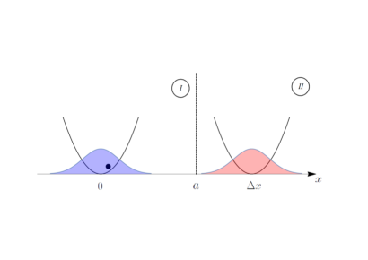
Figure 1: Schematic depiction of the quenched harmonic potential. The initial potential $V(x)$ is centered at $x=0$, whereas the potential after the shift $V_{f}(x)$ is centered around $x=\Delta x$. The vertical line divides between locations belonging to outcomes $I$ and $II$. The filled curves depict the equilibrium probability distribution of the potentials $V$ and $V_{f}$.

Eq. (3) also requires an investigation of a reverse process. In this reverse process the system is initially equilibrated in $V_{f}(x)$. The potential is then changed suddenly to $V(x)$, and the particle location is measured.

The sudden nature of the process means that the system has no time to evolve. All the information about a realization is given by its initial condition, which is sampled out of the equilibrium distribution. There is simply no time to apply feedback. Nevertheless, Eq. (3) holds for realizations with either outcome, for any value of the parameter $a$. We wish to know for what outcome and which value of $a$ the convergence is fastest, and why.

IV.2 Estimation of the number of realization needed for convergence

Let us first give an estimate for the number of realizations needed for convergence in free-energy calculations based on the Jarzynski equality (1). Here there is no measurement and only the forward process is needed. The probability that the particle is initially at $x$ is given by

$$p_{F}(x)=\sqrt{\frac{\beta k}{2\pi}}e^{-\frac{1}{2}\beta kx^{2}}.$$ (16)

When the harmonic potential is suddenly shifted work is done on the particle. This work is given by

$$w(x)=V_{f}(x)-V(x)=\frac{1}{2}k\Delta x^{2}-kx\Delta x.$$ (17)

The so-called dominant realizations, which must be sampled to ensure convergence, were identified by Jarzynski to be the time-reversed of typical realizations of the reverse process Jarzynski (2006). For the simple example considered here the initial equilibrium probability distribution of the reverse process is

$$p_{R}(x)=\sqrt{\frac{\beta k}{2\pi}}e^{-\frac{1}{2}\beta k(x-\Delta x)^{2}},$$ (18)

and therefore the typical realizations in the reverse process are those located near $x\simeq\Delta x$. For $\beta k\Delta x^{2}\gg 1$ these realizations are in the far tail of the distribution $p_{F}(x)$, and are exponentially unlikely. The number of realizations needed for convergence therefore scales like

$$N_{JE}^{*}\sim\frac{1}{p_{F}(\Delta x)}\sim e^{\frac{1}{2}\beta k\Delta x^{2}}.$$ (19)

The symbol $\sim$ is used to mean that these expressions have the same dominant exponential factor, but may differ by slower varying prefactors that may, for instance, includes powers of $\beta k\Delta x^{2}$. We employ such a crude asymptotic approximation since: i) we will not be able to determine the correct prefactor when discussing convergence with a measurement, and ii) we will consider parameter values such that the exponentials are dominant, and knowledge of them will suffice for comparison between alternative calculations.

We turn now to estimate the number of realizations required if one wishes to estimate $\Delta F$ from Eq. (3). It will be instructive to consider calculations employing realizations with outcomes $I$ and $II$ separately. One of the main difference between calculations based on Eq. (3) and on Eq. (1) is that the former requires one to employ both the forward and reverse process. Specifically, the combination $p_{m}\left<e^{-\beta w}\right>_{|m}$ is estimated by repeating the forward process, whereas $p_{m}^{R}$ is obtained from realizations of the reverse process. As discussed in the previous section the costs of both estimates should be taken into account.

Let us first focus on a calculation in which one estimates $\Delta F$ from realizations with outcome $II$. Let us also assume that the parameter $a$ is located in the region between $0$ and $\Delta x$, where $\beta ka^{2},\beta k(a-\Delta x)^{2}\gg 1$. This means that $a$ is in the tails of both $p_{F}(x)$ and $p_{R}(x)$, simplifying many of the estimates in this section.

As discussed in the previous section one requires roughly

$$N_{F,II}^{*,exp}\sim\frac{1}{p_{II}}e^{\beta\left<\Sigma\right>_{II}^{R}}$$

realizations of the forward process to estimate the exponential average $\left<e^{-\beta w}\right>_{|II}$. The total cost of the calculation with the $II$ outcome is therefore given by

$$N_{II}^{*}(a)\sim\frac{1}{p_{II}}e^{\beta\left<\Sigma\right>_{II}^{R}}+\frac{1}{p_{II}^{R}}.$$ (20)

Estimation of $N_{II}^{*}(a)$ is quite straightforward for $a$ values that satisfy $\beta ka^{2},\beta k(a-\Delta x)^{2}\gg 1$. $p_{II}^{R}\simeq 1$ and therefore the difficulty in estimating $\Delta{\cal F}$ is solely due to the forward process. In contrast $p_{II}\sim\exp\left(-\frac{1}{2}\beta ka^{2}\right)\ll 1$ must be considered but this factor appears twice in the estimate. Once as a prefactor, and once in $\left<\Sigma\right>_{|II}^{R}=\left<w\right>_{|II}^{R}+k_{B}T\ln\frac{p_{II}}{p_{II}^{R}}$ The two terms cancel each other. What is left is to estimate $\left<w\right>_{|II}^{R}$, the mean work done by realizations of the reverse process with outcome $II$. Since realizations with outcome $I$ are very rare in the reverse process this amounts to estimating the mean work in this process, for which typical realizations have $x\simeq\Delta x$. As a result $\left<w\right>_{|II}^{R}\simeq V(\Delta x)-V_{f}(\Delta x)=\frac{1}{2}k\Delta x^{2}$. Collecting everything, we find

$$N_{II}^{*}(a)\sim e^{\frac{1}{2}\beta k\Delta x^{2}}\sim N_{JE}^{*}.$$ (21)

We have just found out that for a range of $a$ values the convergence of calculations based on Eq. (3) with outcome $II$ and of calculations based on the Jarzynski equality (1) are equally challenging. Interestingly, convergence of $\left<e^{-\beta w}\right>_{|m}$ in Eq. (3) is faster than that of $\left<e^{-\beta w}\right>$ in Eq. (1), but this is compensated by the fact that most realizations of the forward process will have the wrong outcome. Does this mean that free energy calculation based on Eq. (3) always exhibit the same convergence as calculations based on the Jarzynski equality? No. As we shall shortly see, realizations with the outcome $I$ exhibit very different behavior.

The estimation of convergence for realizations with outcome $I$ proceeds along similar lines. However, in this case $p_{I}=\int_{-\infty}^{a}p_{F}(x)dx\simeq 1$, while $p_{I}^{R}\sim e^{-\frac{1}{2}\beta k(\Delta x-a)^{2}}\ll 1$. In this case the dominant realizations that one must sample to obtain a reasonable estimate for the free energy difference are the most typical realizations of the reverse process subject to the constraint $x\leq a$. These are rare realizations, located in the tail of the probability $p_{R}(x)$. In fact, the Gaussian shape of $p_{R}(x)$ mean that the most typical realizations of the reversed process with the constraint are those with $x\simeq a$. For these realizations the mean dissipated work is roughly

$$\left<w\right>_{|I}^{R}\simeq V(a)-V_{f}(a)=ka\Delta x-\frac{1}{2}k\Delta x^{2}.$$ (22)

The number of realizations required to estimate the combination $p_{I}\left<e^{-\beta w}\right>_{|I}$ is therefore

$$\frac{1}{p_{I}}e^{\beta\left<\Sigma\right>_{I}^{R}}\sim e^{\beta\left<w\right>_{|I}^{R}-\ln p_{I}^{R}}\sim e^{\frac{1}{2}\beta ka^{2}}.$$

Since $p_{I}^{R}\ll 1$ one also requires of the order of $1/p_{I}^{R}$ realizations of the reverse process. The total number of realizations needed for a reasonable estimate of the free energy difference is therefore

$$N_{I}^{*}(a)\sim e^{\frac{1}{2}\beta ka^{2}}+e^{\frac{1}{2}\beta k(\Delta x-a)^{2}},$$ (23)

where the first term comes from the number of times the forward process is performed while the second term comes from the number of times one should realize the reverse process. Considering that $\beta ka^{2},\beta k(\Delta x-a)^{2}\gg 1$ one immediately sees that $N_{I}^{*}(a)$ is minimal when $a=\Delta x/2$. In that case $N_{I}^{*}(\Delta x/2)\sim e^{\frac{1}{8}\beta k\Delta x^{2}}\ll N_{JE}^{*}$. Convergence of free energy estimation based on Eq. (3) is therefore much faster in comparison to that of a calculation based on Eq. (1) when $a=\Delta x/2$ and only realizations with outcome $I$ are used. Convergence is, in fact, accelerated by ignoring realizations with the “unwanted” outcome $II$!!

One can intuitively understand the reasons for different convergence rates of calculations employed realizations with different outcomes by looking at the dominant realizations which one needs to sample in each case. For outcome $II$ the dominant realizations are those with $x\simeq\Delta x$. These are also the dominant realizations in calculations based on the Jarzynski equality (1). These realizations are very unlikely in the forward process, but are typical for the reverse process.

The dominant realizations of the calculation with outcome $I$ are located at $x$ values which are slightly smaller but close to $a$. These are still rare realizations of the forward process, but sampling them is much more likely than sampling realizations with $x\simeq\Delta x$. To obtain the correct free energy difference from realization with this outcome Eq. (3) mandates that the reverse process should also be used and $p_{I}^{R}$ estimated. One also needs realizations with $x\simeq a$ for this purpose. The additional cost of sampling such realizations is large, but also much less than the cost of sampling forward realizations with $x\simeq\Delta x$. The improved convergence is therefore achieved by designing the measurement (by choosing $a$) in a way that modifies the dominant realizations of the process. A good choice of $a$ results in a calculation with dominant realizations that divide the numerical cost between the forward and reverse processes. The nonlinear dependence of this cost on parameters results in a total cost which is much lower than that of a naive calculation based on Eq. (1).

IV.3 Connection to Bennett’s acceptance ratio method

The estimation of the free energy difference based on Eq. (1), which was used as a benchmark in the previous subsection, is somewhat naive. Better convergence can be attained by using the acceptance ratio method proposed by Bennett in 1976 in the context of thermodynamic perturbation theory Bennett (1976). While originally developed for computations in which the Hamiltonian is changed in a sudden manner, the method is applicable also for finite-time processes Shirts et al. (2003); Kim et al. (2012).

The acceptance ratio method is based on the identity Shirts et al. (2003); Bennett (1976)

$$e^{-\beta\Delta{\cal F}}=\frac{\left<f(w)\right>_{F}}{\left<f(-w)e^{-\beta w}\right>_{R}},$$ (24)

which holds for any function $f$. Bennett showed that the statistical variance in estimates of $\Delta{\cal F}$ is minimal when the function $f$ is chosen to be the Fermi function

$$f(w)=\frac{1}{1+\frac{n_{F}}{n_{R}}e^{\beta(w-\Delta{\cal F})}}$$ (25)

where $n_{F}$ and $n_{R}$ are the number of realizations used to sample the forward and reverse process respectively. Shirts et al. demonstrated that the acceptance ratio method emerges from maximum likelihood considerations Shirts et al. (2003).

To make a connection with the model studied here, for which we obtained analytical estimates for number of realizations needed for convergence in Sec. IV.2, we note that the best convergence was achieved when the numerical load was equally divided between the forward and reverse processes. Substituting the Fermi function and $n_{F}=n_{R}$ in Eq. (24), we find

$$e^{-\beta\Delta{\cal F}}=\frac{\left<\frac{1}{1+e^{\beta(\Delta{\cal F}-w)}}e^{-\beta w}\right>_{F}}{\left<\frac{1}{1+e^{\beta(\Delta{\cal F}+w)}}\right>_{R}}.$$ (26)

The Fermi functions in the numerator of Eq. (26) give weights of order unity to realizations of the forward process with $\beta w-\beta\Delta{\cal F}\gg 1$. In contrast, the weights are exponentially small when $\beta w-\beta\Delta{\cal F}\ll-1$. There is a smooth transition between these two regions, which is centered around $w=\Delta{\cal F}$.

For the shifted harmonic oscillator studied in Sec. IV.2 $\Delta{\cal F}=0$. In addition, the sudden dynamics results in a simple connection between the particle’s location and the work done during the process, see Eq. (17). $x=\Delta x/2$ is precisely the point where $w=\Delta F=0$. The region where $w>0$ is equivalent to $x<\Delta x/2$ and similarly $w<0$ for $x>\Delta x/2$. The Fermi function in the numerator of Eq. (26) therefore gives larger weights to points that satisfy $x<\Delta x/2$, that is, to points located in region $I$ ($a=\Delta x/2$). Since the work done in the reverse process is minus the work done in the forward process the Fermi function in the denominator of Eq. (26) also favors points in $I$.

When the Fermi functions in Eq. (26) are replaced by step functions, either by hand, or by lowering the temperature to 0, only realizations with $x<\Delta x/2$ are kept. Realizations with $x>\Delta x/2$ are given vanishing weights and are effectively discarded. Replacement of the Fermi function with a step function therefore replaces Eq. (26) with Eq. (3) for the outcome $m=I$. This reveals that the improved convergence found in Sec. IV.2 is closely connected to Bennett’s acceptance ratio method. Specifically, the nonequilibrium free energy calculation for sudden processes, based on separating realizations according to outcomes, is at best an approximation of Bennett’s acceptance ratio method, in which the only weights used are $0$ or $1$.

V A model of a hairpin pulling experiment

The example studied in Sec. IV was designed to be particularly simple to allow for a derivation of analytical estimates for the number of realizations needed for convergence. This simplification came with a cost. The model had instantaneous dynamics that left no time for the application of feedback. But Eq. (3) holds also for processes with feedback. Interestingly, inclusion of feedback can either improve or hinder the convergence rate. On one hand feedback can be used to make the process more reversible. On the other hand, the time that it takes the system to respond to the feedback is also the time in which the measurement loses some of its predictive value regarding the work accumulated during the realization.

To see how this interplay between effects works in practice we study numerically a model that mimics an experiment in which an RNA hairpin is pulled open Ritort et al. (2002). The pulling process occurs over a finite time interval such that the system has time to respond to changes in the pulling protocol following the measurement. The model we study is chosen to exhibit the characteristic behavior of an actual pulling experiment but is intentionally simplified. This makes it easier to gather sufficient statistics, and more importantly to gain qualitative understanding of its behavior.

V.1 The two state model

Ritort, Bustamante, and Tinoco have used a simple model of a hairpin pulling experiment to study the convergence rate of free energy calculations Ritort et al. (2002). Here we use the same model, but add measurement and feedback to the process. This simple model of a hairpin has only two states. A closed configuration with vanishing length and energy, and an open state with length $l$ and energy $\Delta E_{0}-f\left(t\right)l$. The force $f(t)$ is the external parameter used to drive the system away from thermal equilibrium. The model is depicted qualitatively in Fig. 2. Transitions between the states are assumed to be Markovian, with rates $r_{c\rightarrow o}=1$ and $r_{o\rightarrow c}=\exp\left[\Delta E-f\left(t\right)l\right]$, where we used $\beta=k_{B}T=1$, $\Delta E=5$, and $l=1$. The subscripts stand for ’open’ and ’closed’.

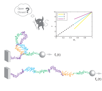
Figure 2: Schematic depiction of a process where an RNA hairpin is pulled open by an external force. The hairpins is modeled as a two state system, and can either be in an open or a closed configuration. A measurement is done in an intermediate time, here $t_{f}/2$, and feedback is applied by changing the pulling force according to the outcome. This change is restricted to a sudden jump in the value of the force, followed by linear variation. Several possible force protocols are depicted in the inset.

The pulling simulation starts from an equilibrium state, with $f\left(0\right)=0$, where the system is very likely to be in the closed state. The force is then increased according to a known protocol in order to open the hairpin. When the system is in the open state work is done on it with rate $\dot{w}=-\dot{f}(t)l$, whereas no work is done when the hairpin is closed. The Jarzynski equality holds for this process, with $\Delta{\cal F}=\ln\left\{\left[1+\exp\left(-\Delta E\right)\right]/\left[1+\exp\left(-\Delta E+f\left(t_{f}\right)l\right)\right]\right\}$. For large final forces $\Delta{\cal F}\approx\Delta E-f\left(t_{f}\right)l$, allowing to easily estimate the binding energy from $\Delta{\cal F}$.

A clear cut comparison of the rate of convergence of free energy calculations with and without measurement and feedback requires knowledge of the optimal driving protocol in each case. However, the optimal driving protocol is not known for the process with feedback. To get a reasonable comparison we restrict ourselves to a one parameter family of protocols. One can then find the best driving protocol by an easy numerical search. The family of driving protocols we chose to use consists of forces that change linearly with time. The duration of the process was chosen to be $t_{f}=1/2$. The initial and final values of the force are always given by $f(0)=0$ and $f(t_{f})=10$.

In all the protocols we have used, the force was initially given by $f(t)=10t/t_{f}$. When measurement and feedback are employed, the state of the system is measured at $t_{m}=t_{f}/2$. Immediately after the measurement the force is changed to a value $f_{+}\equiv f(t_{m}^{+})$. This value is the tunable parameter in the family of driving protocols. At times satisfying $t>t_{m}$ the force is changed linearly until it reaches a protocol independent final value $f(t_{f})=10$ at the end of the process. Several force protocols from this one-parameter family are depicted in the inset of Fig. 2.

The dynamics of the two state system was explored using a kinetic monte-carlo simulation based on the algorithm developed in Ref. Prados et al. (1997). The protocol duration was chosen to be $t_{f}=1/2$. For this duration trajectories typically make few transitions between the states, and some never even make a single transition during the pulling process. One therefore expects that free energy calculations will not converge easily.

V.2 Outcome-work correlations

For the instantaneous process studied in Sec. IV, the measurement outcome was directly related to the work done in the process. In processes with a finite duration, a measurement preformed at a given instance cannot fully determine the work accumulated during the whole process. However, one can expect that the open and closed outcomes will be correlated with the work done in the process due to the different work rate $\dot{w}$ in the two states. The usefulness of the measurement in the context of free energy calculations is therefore related to the degree of correlations between the outcome and work. Our first goal was to investigate this correlation.

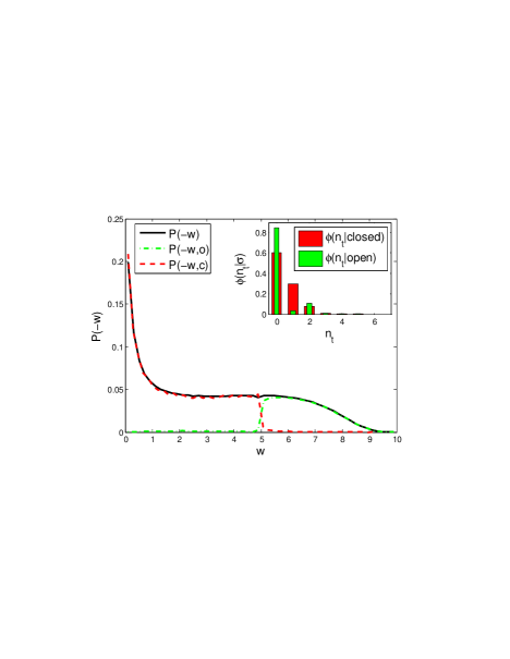
Figure 3: Correlations between work and measurement outcomes. The solid line depicts the continuous part of the work distribution for the linear protocol. The dashed red (grey) and green (light grey) lines depict the joint distribution work and outcome. For the selected parameters there is a clear correlation between the work and measured outcome. Inset: the distribution of the number of transitions made during the process, with realizations separated according to the measurement outcome.

Fig. 3 depicts the continuous part of the work distribution obtained for the linear protocol (with $f_{+}=5$). We note that the distribution also has a discrete part, at values $w=-10,0$, due to trajectories that remain in the initial state throughout the process. These are not shown. Performing a measurement allows to divide this distribution into two pieces, depending on the outcome. They are also depicted in Fig. 3. These marginal distributions of work and outcome are clearly narrower than the full distribution. The narrower work distribution associated with each outcome result in faster convergence rate of the conditional exponential average $\left<e^{-\beta w}\right>_{|m}$ compared to that of $\left<e^{-\beta w}\right>$ without a measurement. It should be clear that measurements that do not result in narrower work distributions, will not be useful as an avenue of accelerating convergence.

The neat division of the work distribution, depicted in Fig. 3, results from the fact that work accumulation is strongly coupled to the state of the system and the relatively short duration of the process. Most of the realizations contributing to the distribution depicted in the figure make a single transition between the states. When this transition precedes the measurement the outcome will be open and the accumulated work will satisfy $w<-5$, and vice versa. The inset depicts the distribution of the number of transitions made in the process, conditioned on the measurement outcome. Nearly $60\%$ of the trajectories starting in the closed state remain there throughout the evolution, highlighting the fact that the system is driven far from equilibrium.

This explanation for the correlations between the measurement outcome and the work done in the process, suggests that there is a tradeoff between the usefulness of measurements and feedback. One expects that the correlations between the outcome and work will be partially erased in slower processes, where typical realizations make many transitions. On the other hand, a longer duration gives the system more time to respond to changes in the force, and thus increases the effectiveness of feedback. For processes with very short duration the situation is reversed. One expect better correlations between outcome and work for judiciously designed measurements. But if the duration of the process is short compared to the typical time between transitions, the system barely reacts to changes in the force. This tradeoff between the utility of measurements and feedback makes it difficult to use feedback to accelerate the convergence rate beyond the improvement due to the inclusion of measurements that was studied in Sec. IV.

V.3 Convergence estimates

The model of the pulling process can be used to test some of the qualitative estimates for convergence discussed in Sec. III in the context of a finite time process. We start by assuming that the probabilities $p_{m}$ and $p_{m}^{R}$ are known. In this case the rate of convergence is determined by the convergence of the exponential average $\left<e^{-\beta w}\right>_{|m}$. Does the convergence of this exponential average behaves like that of calculations based on the Jarzynski equality, with $\left<\Sigma\right>_{m}$ playing the role of the dissipated work?

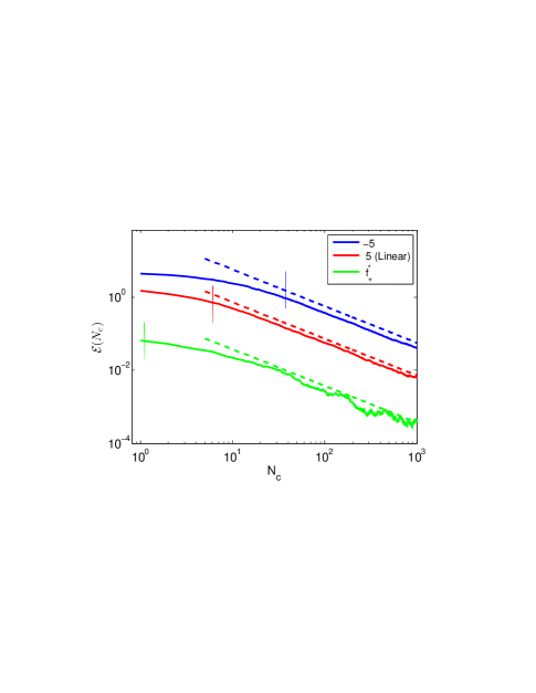
Figure 4: The mean bias ${\cal E}\left(N_{c}\right)$, calculated under the assumption that $p_{c}$ and $p_{c}^{R}$ are known, as a function of the number of realizations with $m=closed$. The dashed lines correspond to the predicted bias for large values of $N_{c}$, where the central theorem applies. The vertical lines depict the estimated number of realizations needed for convergence of $\left<e^{-\beta w}\right>_{|c}$. The blue (upper) line corresponds to $f_{+,c}=-5$, the red (middle) line to the perfectly linear protocol, and the green (lower) line to the protocol with $f_{+,c}=f^{*}$, namely to the protocol with the lowest bias.

Figure 4 depicts the mean bias ${\cal E}\left(N_{c}\right)$ for three different protocols. Since the purpose of the calculation was to examine the convergence rate of the exponential average the calculation was done using the exact values of $p_{c}$ and $p_{c}^{R}$. One of the protocols we used was the completely linear protocol, with $f_{+}=5$ and $\left<\Sigma\right>_{c}\simeq 1.5$. We also studied a protocol that is expected to have poor convergence rate, with $f_{+}=-5$ and $\left<\Sigma\right>_{c}\simeq 4.5$. Finally, we took a protocol with $f_{+,c}^{*}=10$, which (nearly) minimizes $\left<\Sigma\right>_{c}$, with $\left<\Sigma\right>_{c}\simeq 0.07$. Based on the discussion of Sec. III we expect that simulations using this protocol would converge faster than its counterparts.

The results depicted in Fig. 4 indeed show that this optimized protocol performs better in comparison to its counterparts for all values of $N_{c}$. We see no indication that the bias curves in Fig. 4 cross each other. This, combined with the monotonic decrease of ${\cal E}(N)$ with $N$ suggests that ${\cal E}(1)=\left<\Sigma\right>_{c}$ can be used to parameterize the convergence of the exponential average. Lower values of $\left<\Sigma\right>_{c}$ lead to more accurate determination of $\Delta F$ at the same cost. The dashed lines correspond to ${\cal E}\left(N_{c}\right)\approx{\text{V}ar}_{c}\left[\exp\left(-\beta\Sigma\right)\right]/2\beta N_{c}$, which describes the large $N$ regime, where convergence is assured. Finally, the horizontal lines mark the value $N_{c}^{*}=\exp\left(\beta\left\langle\Sigma\right\rangle_{c}^{R}\right)$, suggested as a rough estimate for the number of realizations needed for convergence Jarzynski (2006). One can see that this estimate performs reasonably well for the linear and $f_{+}=-5$ protocols, since it points to the region where the calculated bias (for large $N_{c}$) starts to deviate from the numerically computed bias. In contrast, this estimate for $N_{c}^{*}$ fails for the optimal protocol, but this is expected since in this case $\left<\Sigma\right>_{c}<1$, and the assumptions under which this estimate was derived are violated.

The numerical results depicted in Fig. 4 therefore behave as predicted in the discussion in Sec. III. This supports the notion that the convergence of exponential averages over realizations with a specific measurement outcome behave just like the exponential average in the Jarzynski equality, as long as the role of the dissipated work is played by $\Sigma$.

In many circumstances the probabilities $p_{m}$ and $p_{m}^{R}$ are not known and one must estimate them using realizations of both the forward and reverse process, accordingly. Indeed, in our discussion in Sec. III we included the expected cost of this estimation, see Eq. (15). For the simple example studied in Sec. IV we have found a tradeoff between the number of realizations needed to accurately estimate the relevant quantities from the forward and reverse processes. When one became more efficient, its counterpart became more troublesome. One may wonder whether a similar tradeoff plays a role also for finite time processes that includes feedback.

Fig. 5 depicts results for $N_{F,m}^{*,exp}$ and $N_{R,m}^{*}$ as a function of the feedback parameter $f_{+}$. Results with the closed outcome are depicted in the top panel, whereas results with the open outcome are included in the bottom panel. The results in the top panel exhibit a clear tradeoff, in which $N_{F,c}^{*,exp}$ decrease with increasing $f_{+}$, while $N_{R,c}^{*}$ increases.

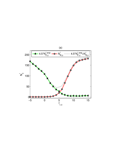
(a)

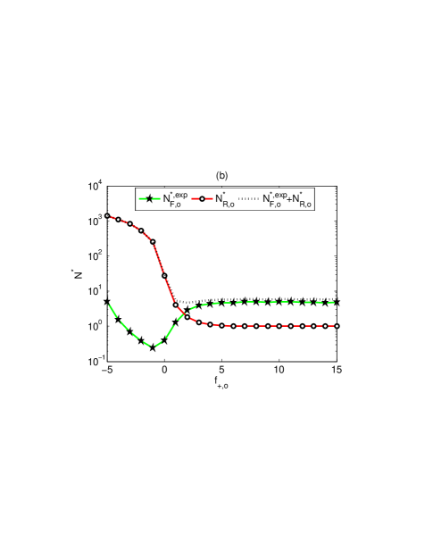
(b)

Figure 5: Estimates of the number of realizations required for convergence of free energy calculations as a function of $f_{+,m}$. The solid-green line with the 5-pointed star symbols is proportional to the number of realizations of the forward process. (See discussion in the main text.) The solid-red line with the ’o’ symbols corresponds to the number of realizations of the reversed process. The dotted line is their sum. The top panel depicts results for realizations with the closed outcome, while the bottom panel includes the estimates for the open outcome.

Let us recall that in Sec. IV realizations with outcome $II$ exhibited a perfect tradeoff in costs, while for realizations with outcome $I$ it was possible to find values of $a$ that divided the cost between the forward and reversed trajectory in a way that reduced the overall numerical cost. Trying to determine which of these types of tradeoffs exist in the current model is tricky. The reason is that we do not know the pre exponential factor of the estimates, and the parameters used in the simulations are not extreme enough to ensure that these pre-exponential factors are irrelevant. Reaching qualitative insights, we chose the numerical prefactor of $N_{F,m}^{*,exp}$ in a way that attempts to create a perfect tradeoff. In the case of the top panel of 5 the sum of costs from the forward and reverse trajectories was chosen to have the same value at the edges of the range of $f_{+}$ values we used. With this somewhat arbitrary choice we expect to find a flat curve in the case of a perfect tradeoff. Instead the curve exhibits a minimum, suggesting that improved convergence is possible in analogy with the results for outcome $I$ in Sec. IV.

The bottom panel of Fig. 5 depicts the estimated number of realizations needed for convergence for a calculation based on the open outcome. For $f_{+,o}>3$ one notices that $N_{F,o}^{*,exp}$ is much larger than $N_{R,o}^{*}$. Moreover, both are essentially constant in this region of parameters. This behavior is essentially identical to the one found for realizations with outcome $II$ in Sec. IV. The qualitative explanation for this behavior is similar as well. The dominant realizations in a calculation based on Eq. (1) will be open at the measurement time. These are the typical realizations in the reverse process. Variation of $f_{+,o}$ in this range has limited ability to change this due to the relatively short duration of the process. As a result the mean work performed in the reverse process does not vary much, and $N_{F,o}^{*,exp}$ is nearly constant.

The behavior is quite different for $f_{+,o}<0$. In this region the probability $p_{o}^{R}$ decreases sharply and as a result the numerical cost of estimating $\Delta{\cal F}$ starts to be dominated by the difficulty to sample the reverse process. The mean work of open trajectories also varies considerably in this region. The decrease of $p_{o}^{R}$ reveals the reason for this behavior. For negative enough values of $f_{+,o}$ typical realizations of the reverse process are no longer open. In this regime feedback is strong enough to modify the dominant realizations needed for an accurate estimate.

Overall, the results presented in Fig. 5 show qualitative behavior that is remarkably similar to the behavior of the shifted harmonic oscillator studied in Sec. IV, despite the obvious differences between the two setups. The fact that the measurement outcome do not fully predict the value of the work does not destroy this similarity due to the correlations depicted in Fig. 3. The ability of feedback to modify the dynamics is mostly seen in extreme values of the parameters, specifically for $f_{+,o}<0$.

V.4 Accuracy of free energy calculations

Fig. 6 highlights the drastic improvement that inclusion of measurement and feedback can achieve if the probabilities $p_{m}$ and $p_{m}^{R}$ are known in advance and do not have to be estimated. The dashed-dotted lines correspond to free-energy calculations based on the Jarzynski equality (1) using several different protocols. The solid line correspond to a calculation based on Eq. (3). It uses results from both measurement outcomes. The protocols of both outcomes were optimized to minimize $\left<\Sigma\right>_{c,o}$, with $f_{+,o}^{*}=8$ and $f_{+,c}^{*}=10$.

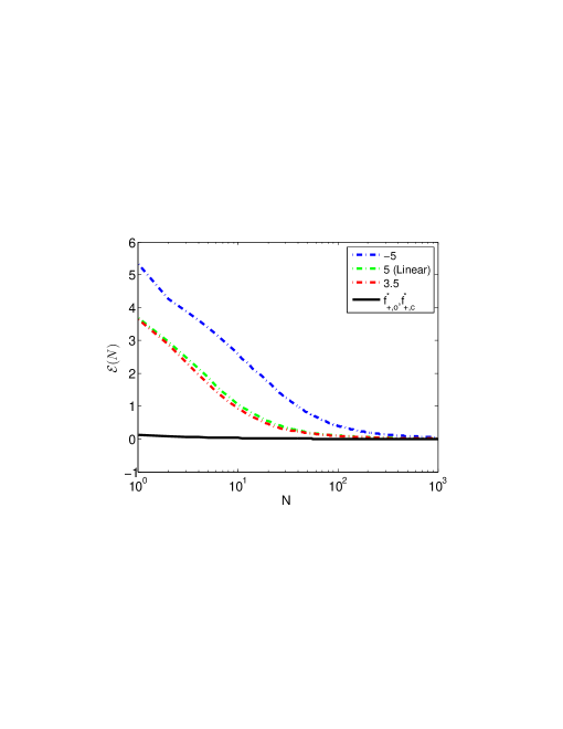
Figure 6: Comparison of the mean bias with and without measurement and feedback. The three dashed-dotted lines depict the mean bias of three calculations based on Eq. (1). Three protocols were used: The green line (second from top) corresponds to the completely linear protocol, while the blue (top) line depicts a protocol with $f_{+}=-5$. The red line (third from top) depicts the results for a protocol optimized for minimal dissipated work $f_{+}=3.5$. The solid-line corresponds for the bias from a calculation with feedback and using Eq. (3). For this curve the force protocols were chosen to minimize $\left<\Sigma\right>_{c,o}$. The calculation was performed under the assumption the values of the probabilities $p_{c,o}$ and $p_{c,o}^{R}$ are known.

When the probabilities are not known, the results presented in Sec. IV suggest that accelerated convergence is possible if one chooses a measurement, outcome, and protocol that divide the difficulty of the calculation between the forward and reverse process. The results depicted in Fig. 5 imply that the closed outcome is the outcome for which such a division is possible.

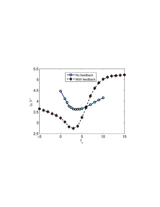
Figure 7: Estimated number of realizations needed for convergence as a function of the jump in the force value immediately after the measurement. The start correspond to the estimated numerical cost of a calculations based on Eq. (3) with $m=closed$. The circles depict the estimated cost of a calculation based on the Jarzynski equality (1).

Fig. 7 compares the estimated number of realizations needed for convergence of calculations based on Eqs. (1) and (3) respectively. The estimate for the calculation with measurement and feedback is composed of the two contributions presented in the top panel of Fig. 5, although they are summed without the prefactor that we included by hand there.

The two estimates shown in Fig. 7 allow to choose protocols that are expected to exhibit the fastest rate of convergence out of all the protocols in the family. For the calculation based on the Jarzynski equality one should therefore choose $f_{+}\simeq 3$. Similarly, for the calculation that is based on Eq. (3) $f_{+,c}\simeq 3.5$ leads to the minimal number of realizations needed for convergence. A comparison of both minima suggests that the calculation which is based on Eq. (3) should be the more accurate of the two.

Fig. 8 compares the mean bias of free energy calculations with several different protocols.

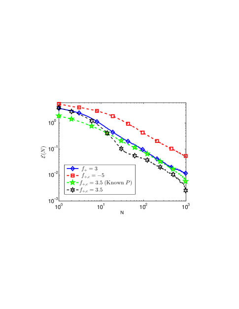
Figure 8: Comparison of the mean bias of the free energy in calculations based on Eq. (1) and Eq. (3). The solid line with the diamond symbols correspond to a calculation based on Eq. (1), with the fastest converging protocol ($f_{+}=3$). The dashed lines all correspond to calculations based on Eq. (3), where only realizations with the closed outcome were used. The red (upper) line with square symbols depict the mean bias for a bad choice of a protocol (with $f_{+,c}-5$). Both the green (lowest) and black curves are obtained for the protocol with $f_{+,c}=3.5$, which is expected be the most accurate based on the estimate depicted in Fig. 7. The green line with 5-pointed star symbols depicts the bias under the assumption that $p_{c}$ and $p_{c}^{R}$ are known. The black curve with 6-pointed star symbols includes also the bias due to the need to estimate these probabilities.

The blue-solid curve with the diamond symbols correspond to a calculation based on the Jarzynski equality (1). The value of $f_{+}=3$ was chosen to minimize the dissipative work in the reverse process. This curve therefore serves as a baseline to which calculations based on Eq. (3) are compared. We note that the bias for the completely linear protocol ($f_{+}=5$) was also calculated, and found to lie almost on top of this curve. The results for the linear protocol were omitted to avoid cluttering the figure.

The dashed lines in Fig. 8 correspond to the bias for several calculations based on Eq. (3). The results of Figs. 5 and 7 suggest that it is best to use realizations with the closed outcome, and that the smallest number of realizations required for convergence is obtained for $f_{+,c}\simeq 3.5$. The curve with $f_{+,c}=-5$ is therefore expected to show comparatively large errors. The results depicted in Fig. 8 indeed show that for this protocol the mean bias is consistently worse than that of the calculation based on Eq. (1). The two other curves correspond to calculations done with a protocol that has $f_{+,c}=3.5$. They are much more accurate as expected.

The black line with 6-pointed stars corresponds to the bias from a calculation that takes into account the need to estimate the probabilities $p_{c}$ and $p_{c}^{R}$. In contrast, the green line with star symbols depicts the bias obtained under the assumption that these probabilities are known. It is presented here to highlight the differences between the two contributions to the bias. Interestingly, for most of the range of $N$ values in the figure the two biases have opposing signs and therefore they partially cancel each other.

A prominent feature of all the curves in Fig. 8 is that they all become parallel to each other for large values of $N$. This expresses the fact that all the biases scale as $C/N$ there. Such scaling is expected due to the central limit theorem, see e.g. the results depicted in Fig. 4.

The results depicted in Fig. 8 show that the bias of the calculations based on Eq. (3) [with $f_{+,c}\simeq 3.5$] is smaller than the bias of a calculation based on Eq. (1). However, the difference between the biases is quite modest. Here it is crucial to note that the results depicted in Fig. 8 were obtained in a parameter regime which is not in the asymptotic region where convergence is exceedingly difficult. Indeed, one sees from Fig. 7 that $N_{c}^{*}\simeq 15$ and $N^{*}\simeq 35$. Moreover, these estimates neglected the role of an unknown prefactor which may be become relevant for not too high values of $N_{c}^{*}$, $N^{*}$. In light of this the modest difference between the two calculations is not unexpected. Based on the qualitative considerations made in Secs. III and IV we expect a much more pronounced difference between the two methods if the parameters are tuned such that $N_{c}^{*}$ and $N^{*}$ are larger by two or more orders of magnitude. Unfortunately, such a numerical investigation will require exponentially more computer resources.

VI Discussion

In this manuscript we have investigated a method of calculating equilibrium free energy differences using repetitions of a nonequilibrium process with measurements and feedback. The method is based on Eq. (3), which allows to calculate $\Delta F$ from realizations with a specific measurement outcome. We have found that improved rate of convergence can be achieved by keeping realizations with one outcome and discarding the rest. While the rate of convergence obtained with this method can be superior to that of a naive calculation using the Jarzynski equality, our results suggest that it may be very difficult to design setups in which the calculation will perform better than calculations employing Bennett’s acceptance ratio method. This conclusion is based on the observation that the method studied here exhibits built in tradeoffs where improved convergence in one part of the calculation makes the estimation of other parts more challenging.

The first of these tradeoffs is related to the way that the separation into different outcomes affect the number of realizations needed to be sampled in the forward and reverse process. The shifted harmonic oscillator studied in Sec. IV clearly exhibits this tradeoff. Free energy calculations based on Eq. (3) require both the forward and reverse processes, just like calculations based on Bennett’s acceptance ratio method. The forward process is used to estimate $p_{m}\left<e^{-\beta w}\right>_{|m}$, while the reverse process is needed to estimate the probability $p_{m}^{R}$. In the case of outcome $II$ ($x>a$), changing $a$ could be used to ease the calculation of the exponential average $\left<e^{-\beta w}\right>_{|II}$, but that came at the expense of a lower value of $p_{II}$. The end result was that one requires the same number of forward realizations. For the other outcome, $x<a$, we found that improved convergence of the forward process came at the expense of slower convergence rate in its reversed counterpart. In this case one could choose the parameter $a$ such that the numerical effort will be divided equally between processes. As discussed in Sec. IV this mechanism of accelerating the convergence rate is based on reweighing of realizations, similar to the mechanism of Bennett’s acceptance ratio method. Crucially, Bennett’s method is designed so that the weights are chosen for minimal variance and maximal statistical likelihood of the estimator, and are therefore superior to the weights used in Eq. (3).

Interestingly, the results presented in Sec. V, obtained for a finite time process with feedback, exhibit qualitatively similar behavior. Fig. 5 shows estimates for the number of realizations needed for convergence of the forward and reverse process. In this case the measurement is fixed, and the parameter which is varied modifies the system’s dynamics. There is no a priori reason to expect behavior that is similar to the one encountered in Sec. IV. Nevertheless, the results presented in the top panel Fig. 5 (for $m=closed$) exhibit qualitatively similar behavior to that of realizations with outcome $I$ in Sec. IV. Similarly, the results depicted in the bottom panel of Fig. 5 (for $m=open$) are qualitatively similar to those found for $x>a$ in Sec. IV, at least for $f_{+}>0$. Crucially, the dominant trajectories needed for convergence of calculation based on Eq. (1) are ones with $m=open$ and $x>a$ in both setups. This suggests that the qualitative similarity of the tradeoffs is not accidental. It is rather related to whether the trajectories that are conditioned to a certain outcome include the set of dominant trajectories of the calculation based on Eq. (1), or not. In the latter case, the restriction to a specific outcome results in a new group of dominant trajectories that are consistent with the outcome.

The second tradeoff is between the usefulness of the weights assigned to realizations and the feedback. Keeping only realizations with a specific outcome is a way of reweighing realizations that uses only the weights $0$ and $1$. From the considerations leading to the Bennett’s acceptance ratio method, a good choice of the weights should depend on the work done in each realization. In the current method the weights are based on the outcome rather than on the work, relying on the strong coupling between the two at short time-scales. For process of short duration the outcome and work can be correlated, suggesting that one can design a measurement that would in principle result in weights that are similar to those of the acceptance ratio method. But short duration also means lack of time to respond to feedback. For processes with long duration the situation is reversed. The dynamics has ample time to respond to changes in parameters, but this comes at the cost of reduced correlations between the outcome and work. This hurts the efficiency of assigning outcome-based weights to realizations.

The results collected in Secs. IV and V suggest that nonequilibrium free energy calculations based on Eq. (3) can show increased convergence rate compared to naive calculations based on the Jarzynski equality (1). However, they are unlikely to perform better than calculations employing Bennett’s acceptance ratio method in repetitions of a single experiment. The underlying reason is that the method uses the weights $0$ and $1$, whereas the acceptance ratio method employees a continuous set of weights, that are chosen to result in the maximal likelihood estimator, which also exhibits the minimal variance. An opposite conclusion may appear considering setups in which the probabilities $p_{m}$ and $p_{m}^{R}$ are known from other sources. For instance if one can solve a master or Fokker-Planck equation for the evolution of the probability distribution, or alternatively run an experiment over many copies of the system at the same time. If the probabilities are known one can design the driving protocol to minimize $\left<\Sigma\right>_{m}$, thereby reducing the difficulty of performing the exponential average. In such cases one should expect drastic improvement in the convergence rate, as is depicted in Fig. 6.

Finally, the qualitative understanding regarding the convergence developed here suggests a more promising approach for the inclusion of measurement and feedback in nonequilibrium free-energy calculations. It is desirable to use optimally chosen weights for any choice of feedback. This may be possible for in the case of measurements with finite errors. A version of the fluctuation theorem holds for such process Sagawa and Ueda (2010); Horowitz and Vaikuntanathan (2010),

$$\left<e^{-\beta w-I}\right>=e^{-\beta\Delta F}.$$

This suggests that one can modify the arguments leading to Bennett’s acceptance ratio so they would hold for this pair of forward and reverse process. The resulting weights would be a function of $\beta w+I$ instead of $\beta w$. The crucial point is that this is a good choice of weights irrespectively of the driving protocol. One can then design feedback that makes the process as reversible as possible. Horowitz and Parrondo Horowitz and Parrondo (2011) demonstrated that in certain cases processes with measurement and feedback can be fully reversible.

Such reversibility is likely to be out of reach for processes whose purpose is to forcibly change the system configuration in a finite time, such as the pulling process of Sec. V. Nevertheless, it will be of great interest to find out by how much one can reduce the dissipation of a process by the addition of an optimally chosen measurement and feedback, and by how much such a procedure accelerates the convergence rate of free energy calculations. The investigation of this alternative approach is left for future work.