Spectral density of mixtures of random density matrices for qubits

Abstract

We derive the spectral density of the equiprobable mixture of two random density matrices of a two-level quantum system. We also work out the spectral density of mixture under the so-called quantum addition rule. We use the spectral densities to calculate the average entropy of mixtures of random density matrices, and show that the average entropy of the arithmetic-mean-state of $n$ qubit density matrices randomly chosen from the Hilbert-Schmidt ensemble is never decreasing with the number $n$. We also get the exact value of the average squared fidelity. Some conjectures and open problems related to von Neumann entropy are also proposed.
 
Keywords. Horn’s problem; probability density function; random quantum state; probabilistic mixture

 
 

1 Introduction

In the early 1950s, physicists had reached the limits of deterministic analytical techniques for studying the energy spectra of heavy atoms undergoing slow nuclear reactions. It is well-known that a random matrix with appropriate symmetries might serve as a suitable model for the Hamiltonian of the quantum mechanical system that describes the reaction [1]. The eigenvalues of this random matrix model the possible energy levels of the system [2]. In quantum statistical mechanics, the canonical states of the system under consideration are the reduced density matrices of the uniform states on a subspace of system and environment. Moreover, such reduced density matrices can be realized by Wishart matrix ensemble [3]. Thus investigations by using random matrix theoretical techniques can lead to deeper insightful perspectives on some problems in Quantum Information Theory [4, 5, 6, 7, 8, 9, 10]. In fact, most works using RMT as a tool to study quantum information theory are concentrated on the limiting density and their asymptotics. In stark contrast, researchers obtained an exact probability distribution of eigenvalues of a multipartite random quantum state via deep mathematical tools such as symplectic geometric method albeit the used definition of Duistermaat-Heckman measure is very abstract and difficult [11, 12]. Besides, the authors conducted exact and asymptotic spectral analysis of the difference between two random mixed quantum states [13]. Non-asymptotic results about average quantum coherence for a random quantum state [14, 15, 16] and its typicality were obtained recently. Motivated by the connection of the works [11, 12] and Horn’s problem [17], we focus the spectral analysis of mixture of several random states in a two-level system. Although the spectral analysis of superposition of random pure states were performed recently [18, 19], the topic about the spectral densities for mixtures of random density matrices from two quantum state ensembles is rarely discussed previously.

Along this line, we will make an attempt toward exact spectral analysis of two kinds of mixtures of two random density matrices for qubits: a) equiprobable mixture of two random density matrices, based on the results obtained in Ref. [17], and b) mixture of two random density matrices under the quantum addition rule (see Definition 3.4, [20]). To the best of our knowledge, such kind of spectral analysis for mixture of random states is rarely conducted, in particular the spectral density under the quantum addition rule. The aim of this work is to analyze properties of a generic quantum state on two-dimensional Hilbert space. For two random states chosen from two unitary orbits, each distributed according to Haar measure over $\mathrm{S}\mathrm{U}(2)$, we derive the spectral density of the equiprobable mixture of both random density matrices for qubits, and the spectral density of mixture of both random density matrices under the quantum addition rule. When they are distributed according to the Hilbert-Schmidt measure in the set $\mathrm{D}\left(\mathbb{C}^{2}\right)$, i.e., the set of all $2\times 2$ density matrices, of quantum states of dimension two, we can calculate the average entropy of ensemble generated by two kinds of mixtures. We also study entropy inequality under the quantum addition rule.

The paper is organized as follows: In Section 2, we recall some useful facts about a qubit. Then we present our main results with their proofs in Section 3. Specifically, we obtain the spectral densities of two kinds of mixtures of two qubit density matrices: (a) the equiprobable mixture and (b) the mixture under the quantum addition rule. By using the relationship between an eigenvalue of a qubit density matrix and the length of its Bloch vector representation, we get compact forms (Theorem 3.2 and Theorem 3.7) of corresponding spectral densities. We also investigate a quantum Jensen-Shannon divergence-like quantity, based on the mixture of two random density matrices under the quantum addition rule. It provide a universal lower bound for the quantum Jensen-Shannon divergence. However our numerical experiments show that such lower bound cannot define a true metric. Next, in Section 4, we use the obtained results in the last section to calculate the average entropies of mixtures of two random density matrices in a two-level quantum system. We show that the average entropy of the arithmetic-mean-state of $n$ qubit density matrices being randomly chosen from the Hilbert-Schmidt ensemble is never decreasing with $n$. As further illumination of our results, we make an attempt to explain why ’mixing reduces coherence’. We also work out the exact value of the average squared fidelity, studied intensively by K. Życzkowski. Finally, we conclude this paper with some remarks and open problems.

2 Preliminaries

To begin with, we recall some facts about a qubit. Any qubit density matrix can be represented as

$$\rho(\boldsymbol{r})=\frac{1}{2}(\mathbb{I}_{2}+\boldsymbol{r}\cdot\boldsymbol{\sigma}),$$ (2.1)

where $\boldsymbol{r}=(r_{x},r_{y},r_{z})\in\mathbb{R}^{3}$ is the Bloch vector with $r:=\left\lvert\mspace{1.0mu}\boldsymbol{r}\mspace{1.0mu}\right\rvert\leqslant 1$, and $\boldsymbol{\sigma}=(\sigma_{x},\sigma_{y},\sigma_{z})$. Here

$$\sigma_{x}=\left(\begin{array}[]{cc}0&1\\ 1&0\end{array}\right),\sigma_{y}=\left(\begin{array}[]{cc}0&-\mathrm{i}\\ \mathrm{i}&0\end{array}\right),\sigma_{z}=\left(\begin{array}[]{cc}1&0\\ 0&-1\end{array}\right)$$

are three Pauli matrices. The eigenvalues of a qubit density matrix are given by: $\lambda_{\pm}(\rho)=\frac{1}{2}\left(1\pm r\right)$, where $r\in[0,1]$. This leads to the von Neumann entropy of the qubit $\rho(\boldsymbol{r})$ of Bloch vector $\boldsymbol{r}$:

$$\mathrm{S}(\rho(\boldsymbol{r}))=\mathrm{H}_{2}\left(\frac{1-r}{2}\right):=\Phi(r),$$ (2.3)

where $\mathrm{H}_{2}\left(p\right)=-p\log_{2}p-(1-p)\log_{2}(1-p)$ for $p\in[0,1]$ is the binary entropy function.

Note that the maximal eigenvalue $\lambda_{+}(\rho)$ for a random qubit density matrix, induced from taking partial trace over a Haar-distributed pure two-qubit state, is subject to the following distribution [11]:

$$\mathrm{d}P(x)=24\left(x-\frac{1}{2}\right)^{2}\mathrm{d}x,$$ (2.4)

where $x:=\lambda_{+}(\rho)\in[1/2,1]$. Since $\lambda_{+}(\rho)=\frac{1}{2}(1+r)$, it follows that the probability density of the length $r$ of Bloch vector of a random qubit $\rho(\boldsymbol{r})$ is summarized into the following proposition.

Proposition 2.1.

The probability density for the length $r$ of the Bloch vector $\boldsymbol{r}$ in the Bloch representation (2.1) of a random qubit $\rho$ by partial-tracing other qubit system over a Haar-distributed pure two-qubit state, is given by

$$p_{r}(r)=3r^{2},\quad r\in[0,1].$$ (2.5)

Furthermore, the probability distribution of Bloch vector $\boldsymbol{r}$ is given by the formula: $p(\boldsymbol{r})[\mathrm{d}\boldsymbol{r}]=3r^{2}\mathrm{d}r\times\frac{1}{4\pi}\delta(1-\left\lvert\mspace{1.0mu}\boldsymbol{u}\mspace{1.0mu}\right\rvert)[\mathrm{d}\boldsymbol{u}]$, where $\delta$ is the Dirac delta function and $[\mathrm{d}\boldsymbol{u}]$ is the Lebesgue volume element in $\mathbb{R}^{3}$.

3 Main results

3.1 The spectral density of equiprobable mixture of two qubit states

For $w\in[0,1]$, we have the probabilistic mixture of two density matrices in a two-level system: $\rho_{w}(\boldsymbol{r})=w\rho(\boldsymbol{r}_{1})+(1-w)\rho(\boldsymbol{r}_{2})$. In particular, for $w=1/2$, we have the equiprobable mixture, that is, $\rho(\boldsymbol{r})=\frac{\rho(\boldsymbol{r}_{1})+\rho(\boldsymbol{r}_{2})}{2}$, hence $\boldsymbol{r}=\frac{\boldsymbol{r}_{1}+\boldsymbol{r}_{2}}{2}$. As in [17], denote $\mu,\nu\in[0,1/2]$ the minimal eigenvalues of two qubit states $\rho(\boldsymbol{r}_{1})$ and $\rho(\boldsymbol{r}_{2})$, respectively. Then we have $\mu=\frac{1-r_{1}}{2}$ and $\nu=\frac{1-r_{2}}{2}$ for $r_{1},r_{2}\in[0,1]$. Denote $\mathcal{O}_{\mu}:=\left\{U\mathrm{diag}(1-\mu,\mu)U^{\dagger}:U\in\mathrm{S}\mathrm{U}(2)\right\}$. We consider the equiprobable mixture of two random density matrices $\rho(\boldsymbol{r}_{1})\in\mathcal{O}_{\mu}$ and $\rho(\boldsymbol{r}_{2})\in\mathcal{O}_{\nu}$. In [17], we have already derived the analytical formula for the spectral density of such equiprobable mixture. This result can be summarized into the following proposition.

Proposition 3.1 ([17]).

The probability density function of an eigenvalue $\lambda$ of the equiprobable mixture of two random density matrices, chosen uniformly from respective unitary orbits $\mathcal{O}_{\mu}$ and $\mathcal{O}_{\nu}$ with $\mu,\nu$ are fixed in $(0,1/2)$, is given by

$$p(\lambda|\mu,\nu)=\frac{\left\lvert\mspace{1.0mu}\lambda-\frac{1}{2}\mspace{1.0mu}\right\rvert}{\left(\frac{1}{2}-\mu\right)\left(\frac{1}{2}-\nu\right)},$$ (3.1)

where $\lambda\in[T_{0},T_{1}]\cup[1-T_{1},1-T_{0}]$. Here $T_{0}:=\frac{\mu+\nu}{2}$ and $T_{1}:=\frac{1-\left\lvert\mspace{1.0mu}\mu-\nu\mspace{1.0mu}\right\rvert}{2}$.

Note that $\lambda\in[T_{0},T_{1}]\cup[1-T_{1},1-T_{0}]$ indicates that the domain of an eigenvalue of the equiprobable mixture: $\frac{1}{2}\left(U\mathrm{diag}(1-\mu,\mu)U^{\dagger}+V\mathrm{diag}(1-\nu,\nu)V^{\dagger}\right)$, where $U,V\in\mathrm{S}\mathrm{U}(2)$.

Given two random density matrices $\rho(\boldsymbol{r}_{1})\in\mathcal{O}_{\mu}$ and $\rho(\boldsymbol{r}_{2})\in\mathcal{O}_{\nu}$. We also see that the eigenvalues of the mixture $\rho(\boldsymbol{r})$ are given by $\lambda=\frac{1\pm r}{2}$ . The sign $\pm$ depends on the relationship between $\lambda$ and $1/2$. Indeed, $\lambda=\frac{1+r}{2}$ if $\lambda\geqslant 1/2$; $\lambda=\frac{1-r}{2}$ if $\lambda\leqslant 1/2$. By using the triple $(r_{1},r_{2},r)$ instead of $(\mu,\nu,\lambda)$, we have the following result.

Theorem 3.2.

The conditional probability density function of the length $r$ of the Bloch vector $\boldsymbol{r}$ of the equiprobable mixture: $\rho(\boldsymbol{r})=\frac{\rho(\boldsymbol{r}_{1})+\rho(\boldsymbol{r}_{2})}{2}$, where $r_{1},r_{2}\in(0,1)$ are fixed, is given by

$$p(r|r_{1},r_{2})=\frac{2r}{r_{1}r_{2}},$$ (3.2)

where $r\in[r_{-},r_{+}]$ with $r_{-}:=\frac{\left\lvert\mspace{1.0mu}r_{1}-r_{2}\mspace{1.0mu}\right\rvert}{2}$ and $r_{+}:=\frac{r_{1}+r_{2}}{2}$.

Denote by $\theta$ the angle between Bloch vectors $\boldsymbol{r}_{1}$ and $\boldsymbol{r}_{2}$ from two random density matrices $\rho(\boldsymbol{r}_{1})\in\mathcal{O}_{\mu}$ and $\rho(\boldsymbol{r}_{2})\in\mathcal{O}_{\nu}$, respectively. Apparently $\theta\in[0,\pi]$. Since $\rho(\boldsymbol{r})=\frac{\rho(\boldsymbol{r}_{1})+\rho(\boldsymbol{r}_{2})}{2}$, i.e., $\boldsymbol{r}=\frac{\boldsymbol{r}_{1}+\boldsymbol{r}_{2}}{2}$, it follows that $r=\frac{1}{2}\sqrt{r^{2}_{1}+r^{2}_{2}+2r_{1}r_{2}\cos\theta}$, where $\theta\in[0,\pi]$.

Clearly the rhs is the invertible function of the argument $\theta$ defined over $[0,\pi]$ when $r_{1}$ and $r_{2}$ are fixed. In view of this, we see that the angle between two random Bloch vectors has the following probability density:

$$f(\theta)=\frac{1}{2}\sin\theta,\quad\theta\in[0,\pi].$$ (3.3)

3.2 The quantum addition rule for two qubit states

Shannon’s Entropy Power Inequality mainly deals with the concavity of an entropy function of a continuous random variable under the scaled addition rule: $f\left(\sqrt{w}X+\sqrt{1-w}Y\right)\geqslant wf(X)+(1-w)f(Y)$, where $w\in[0,1]$ and $X,Y$ are continuous random variables and the function $f$ is either the differential entropy or the entropy power [21]. Some generalizations in the quantum regime along this line are obtained recently. For instance, quantum analogues of these inequalities for continuous-variable quantum systems are obtained, where $X$ and $Y$ are replaced by bosonic fields and the addition rule is the action of a beam splitter with transmissivity $w$ on those fields [21, 22]. Similarly, Audenaert et al establish a class of entropy power inequality analogs for qudits. The addition rule used in these inequalities is given by the so-called partial swap channel [20]. Let us recall some notions we will use in this paper.

Let $\{|j\rangle:j=1,\ldots,d\}$ be the standard basis of $\mathbb{C}^{d}$. Then $\{|ij\rangle:i,j=1,\ldots,d\}$ is an orthonormal basis of $\mathbb{C}^{d}\otimes\mathbb{C}^{d}$. Denote by $\mathrm{D}\left(\mathbb{C}^{d}\right)$ the set of all density matrices on $\mathbb{C}^{d}$. The swap operator $S\in\mathrm{U}(\mathbb{C}^{d}\otimes\mathbb{C}^{d})$, the unitary group on $\mathbb{C}^{d}\otimes\mathbb{C}^{d}$, is defined through its action on the basis vectors $|ij\rangle$ as follows: $S|ij\rangle=|ji\rangle$ for all $i,j=1,\ldots,d$. Explicitly, the swap operator can be rewritten as $S=\sum^{d}_{i,j=1}|ij\rangle\langle ji|$. From the definition of the swap operator, we see that $S$ is self-adjoint and unitary. Audenaert et al defined a qudit partial swap operator as a unitary interpolation between the identity and the swap operator in [20].

Definition 3.3 (Partial swap operator).

For $t\in[0,1]$, the partial swap operator $U_{t}\in\mathrm{U}(\mathbb{C}^{d}\otimes\mathbb{C}^{d})$ is the unitary operator $U_{t}:=\sqrt{t}\mathbb{I}_{d}\otimes\mathbb{I}_{d}+\sqrt{1-t}\mathrm{i}S$.

It is easily seen that the matrix representation of the partial swap operator for the two-level system is

$$U_{t} = \left[\begin{array}[]{cccc}\sqrt{t}+\mathrm{i}\sqrt{1-t}&0&0&0\\ 0&\sqrt{t}&\mathrm{i}\sqrt{1-t}&0\\ 0&\mathrm{i}\sqrt{1-t}&\sqrt{t}&0\\ 0&0&0&\sqrt{t}+\mathrm{i}\sqrt{1-t}\end{array}\right].$$

When $t=1/2$, we have

$$U_{1/2} = \frac{1}{\sqrt{2}}\left[\begin{array}[]{cccc}1+\mathrm{i}&0&0&0\\ 0&1&\mathrm{i}&0\\ 0&\mathrm{i}&1&0\\ 0&0&0&1+\mathrm{i}\end{array}\right],$$

Consider a family of CPTP maps $\mathcal{E}_{t}:\mathrm{D}\left(\mathbb{C}^{d}\otimes\mathbb{C}^{d}\right)\to\mathrm{D}\left(\mathbb{C}^{d}\right)$ parameterized by $t\in[0,1]$. It is defined in terms of the partial swap operator $U_{t}$ in the above definition. For any $\rho_{12}\in\mathrm{D}\left(\mathbb{C}^{d}\otimes\mathbb{C}^{d}\right)$, let $\mathcal{E}_{t}(\rho_{12})=\operatorname{Tr}_{2}\left(U_{t}\rho_{12}U^{\dagger}_{t}\right)$. Denote $\widehat{\mathcal{E}}_{t}(\rho_{12})=\operatorname{Tr}_{1}\left(U_{t}\rho_{12}U^{\dagger}_{t}\right)$. We are particularly interested in the case where the input state $\rho_{12}$ is a product state, i.e. $\rho_{12}=\rho_{1}\otimes\rho_{2}$ for $\rho_{j}\in\mathrm{D}\left(\mathbb{C}^{d}\right),j=1,2$. Apparently, $S(\rho_{1}\otimes\rho_{2})S=\rho_{2}\otimes\rho_{1}$. Now

$$U_{t}(\rho_{1}\otimes\rho_{2})U^{\dagger}_{t}=t\rho_{1}\otimes\rho_{2}+(1-t)\rho_{2}\otimes\rho_{1}+\mathrm{i}\sqrt{t(1-t)}[S,\rho_{1}\otimes\rho_{2}].$$ (3.6)

From this, we see easily that

$$\mathcal{E}_{t}(\rho_{1}\otimes\rho_{2}) = t\rho_{1}+(1-t)\rho_{2}-\mathrm{i}\sqrt{t(1-t)}[\rho_{1},\rho_{2}],$$ (3.7)

$$\widehat{\mathcal{E}}_{t}(\rho_{1}\otimes\rho_{2}) = t\rho_{2}+(1-t)\rho_{1}+\mathrm{i}\sqrt{t(1-t)}[\rho_{1},\rho_{2}].$$ (3.8)

In particular, for $t=\frac{1}{2}$, we get

$$\mathcal{E}_{1/2}(\rho_{1}\otimes\rho_{2}) = \frac{1}{2}\left(\rho_{1}+\rho_{2}-\mathrm{i}[\rho_{1},\rho_{2}]\right),$$ (3.9)

$$\widehat{\mathcal{E}}_{1/2}(\rho_{1}\otimes\rho_{2}) = \frac{1}{2}\left(\rho_{1}+\rho_{2}+\mathrm{i}[\rho_{1},\rho_{2}]\right).$$ (3.10)

Definition 3.4 (Quantum addition rule).

For any $t\in[0,1]$ and any $\rho_{1},\rho_{2}\in\mathrm{D}\left(\mathbb{C}^{d}\right)$, we define $\rho_{1}\boxplus_{t}\rho_{2}:=\mathcal{E}_{t}(\rho_{1}\otimes\rho_{2})$. It is trivial that $\rho_{2}\boxplus_{t}\rho_{1}=\widehat{\mathcal{E}}_{t}(\rho_{1}\otimes\rho_{2})$.

Denote $g_{d}(t):=\mathrm{S}(\rho_{1}\boxplus_{t}\rho_{2})+\mathrm{S}(\rho_{2}\boxplus_{t}\rho_{1})-\mathrm{S}(\rho_{1})-\mathrm{S}(\rho_{2})$, where $\mathrm{S}(\rho)$ is the von Neumann entropy of $\rho$. This can be viewed as the mutual information between two $d$-level subsystems after performing $\mathcal{E}_{t}$ when their composite system lives in the product form. In other words, such quantity $g_{d}(t)$ stands for the correlative power of the partial swap channel $\mathcal{E}_{t}$, we conjecture $\max_{t\in[0,1]}g_{d}(t)=g_{d}(1/2)$ for any $d\geqslant 2$, that is, the correlative power of the partial swap channel achieves its maximum at $t=1/2$. We next give a positive answer to this conjecture in the qubit case. The proof for the qudit case is expected.

Proposition 3.5.

For any $t\in[0,1]$ and any two qubit density matrices $\rho_{1},\rho_{2}\in\mathrm{D}\left(\mathbb{C}^{2}\right)$, we have

$$\max_{t\in[0,1]}g_{2}(t)=g_{2}(1/2).$$ (3.11)

That is,

$$\max_{t\in[0,1]}\left(\mathrm{S}(\rho_{1}\boxplus_{t}\rho_{2})+\mathrm{S}(\rho_{2}\boxplus_{t}\rho_{1})\right)=2\mathrm{S}(\rho_{1}\boxplus_{1/2}\rho_{2}).$$ (3.12)

Proof.

Denote $s(t)=\mathrm{S}(\rho_{1}\boxplus_{t}\rho_{2})+\mathrm{S}(\rho_{2}\boxplus_{t}\rho_{1})$. Thus $s(t)=\Phi(r_{12}(t))+\Phi(r_{21}(t))$, where

$$\Phi(x)=-\frac{1+x}{2}\log_{2}\frac{1+x}{2}-\frac{1-x}{2}\log_{2}\frac{1-x}{2},$$

and $r_{12}(t)=\left\lvert\mspace{1.0mu}\boldsymbol{r}(\rho_{1}\boxplus_{t}\rho_{2})\mspace{1.0mu}\right\rvert,r_{21}(t)=\left\lvert\mspace{1.0mu}\boldsymbol{r}(\rho_{2}\boxplus_{t}\rho_{1})\mspace{1.0mu}\right\rvert$. Then

$$s^{\prime}(t)=\frac{1}{2}r^{\prime}_{12}(t)\log_{2}\frac{1-r_{12}(t)}{1+r_{12}(t)}+\frac{1}{2}r^{\prime}_{21}(t)\log_{2}\frac{1-r_{21}(t)}{1+r_{21}(t)}$$

and

$$s^{\prime\prime}(t) = \frac{1}{2}r^{\prime\prime}_{12}(t)\log_{2}\frac{1-r_{12}(t)}{1+r_{12}(t)}+\frac{1}{2}r^{\prime\prime}_{21}(t)\log_{2}\frac{1-r_{21}(t)}{1+r_{21}(t)}$$

$$-\frac{1}{\ln 2}\left(\frac{[r^{\prime}_{12}(t)]^{2}}{1-r_{12}(t)^{2}}+\frac{[r^{\prime}_{21}(t)]^{2}}{1-r_{21}(t)^{2}}\right).$$

Note that $0\leqslant r_{12}(t)\leqslant tr_{1}+(1-t)r_{2}\leqslant 1$ and $0\leqslant r_{21}(t)\leqslant(1-t)r_{1}+tr_{2}\leqslant 1$ because $r_{1},r_{2}\in[0,1]$. Thus

$$-\frac{1}{\ln 2}\left(\frac{[r^{\prime}_{12}(t)]^{2}}{1-r_{12}(t)^{2}}+\frac{[r^{\prime}_{21}(t)]^{2}}{1-r_{21}(t)^{2}}\right)<0.$$

Denote $\alpha:=2r_{1}r_{2}\cos\theta+r^{2}_{1}r^{2}_{2}\sin^{2}\theta$ and $\varphi(t)=(r^{2}_{1}+r^{2}_{2}-\alpha)t^{2}+\alpha t$. Hence

$$r_{12}(t)=\sqrt{\varphi(t)-2r^{2}_{2}t+r^{2}_{2}},\quad r_{21}(t)=\sqrt{\varphi(t)-2r^{2}_{1}t+r^{2}_{1}}.$$

This implies that $r^{\prime}_{12}(t)=\frac{\varphi^{\prime}(t)-2r^{2}_{2}}{2r_{12}(t)}$. Based on this, we obtain

$$r^{\prime\prime}_{12}(t)=\frac{2\varphi^{\prime\prime}(t)r^{2}_{12}(t)-\left(\varphi^{\prime}(t)-2r^{2}_{2}\right)^{2}}{4r^{3}_{12}(t)}.$$

By using $\varphi^{\prime}(t),\varphi^{\prime\prime}(t)$, and $r^{2}_{12}(t)$, we have

$$2\varphi^{\prime\prime}(t)r^{2}_{12}(t)-\left(\varphi^{\prime}(t)-2r^{2}_{2}\right)^{2} = 4r^{2}_{2}(r^{2}_{1}+r^{2}_{2}-\alpha)-(\alpha-2r^{2}_{2})^{2}$$

$$= r^{2}_{1}r^{2}_{2}\left(4-(2\cos\theta+r_{1}r_{2}\sin^{2}\theta)^{2}\right)\geqslant 0,$$

implying $r^{\prime\prime}_{12}(t)>0$. Similarly, we see that $r^{\prime\prime}_{21}(t)>0$. In summary, we get that $s^{\prime\prime}(t)<0$. That is, $s(t)$ is the strict concave function over $[0,1]$. It is easily seen that $r_{12}(1/2)=r_{21}(1/2)=\sqrt{\varphi(1/2)}$. Now $r^{\prime}_{12}(1/2)=\frac{\varphi^{\prime}(1/2)-2r^{2}_{2}}{2r_{12}(1/2)}$ and $r^{\prime}_{21}(1/2)=\frac{\varphi^{\prime}(1/2)-2r^{2}_{1}}{2r_{12}(1/2)}$. Apparently $\varphi^{\prime}(1/2)=r^{2}_{1}+r^{2}_{2}$ by the expression of $\varphi$. Substituting $r_{12}(1/2),r^{\prime}_{12}(1/2),\varphi^{\prime}(1/2)$ into the expression of $s^{\prime}(1/2)$ gives rise to the result: $s^{\prime}(1/2)=0$. Therefore the maximum of $s(t)$ on $[0,1]$ is taken at $1/2$, i.e., $\max_{t\in[0,1]}s(t)=s(1/2)$. This is equivalent to the desired conclusion $\max_{t\in[0,1]}g_{2}(t)=g_{2}(1/2)$. We are done. ∎

The result in Proposition 3.5 can be viewed as another proof of the following inequality:

$$\mathrm{S}(\rho_{1}\boxplus_{1/2}\rho_{2})\geqslant\frac{1}{2}\mathrm{S}(\rho_{1})+\frac{1}{2}\mathrm{S}(\rho_{2}).$$

We also have the following interesting result:

Proposition 3.6.

In a two-level system, it holds that

$$w\mathrm{S}(\rho_{1})+(1-w)\mathrm{S}(\rho_{2}) \leqslant \mathrm{S}(\rho_{1}\boxplus_{w}\rho_{2})$$ (3.13)

$$\leqslant \mathrm{S}\left(w\rho_{1}+(1-w)\rho_{2}\right)$$ (3.14)

for any weight $w\in[0,1]$. In particular, for $w=1/2$, we have

$$\frac{\mathrm{S}(\rho_{1})+\mathrm{S}(\rho_{2})}{2}\leqslant\mathrm{S}(\rho_{1}\boxplus_{1/2}\rho_{2})\leqslant\mathrm{S}\left(\frac{\rho_{1}+\rho_{2}}{2}\right).$$ (3.15)

Proof.

The inequality in (3.13) is obtained in [20]. In order to prove the second one in (3.14), we use Bloch representation of a density matrix for a qubit state, for $w\in[0,1]$,

$$\rho(\boldsymbol{r}(w)) := w\rho(\boldsymbol{r}_{1})+(1-w)\rho(\boldsymbol{r}_{2}),$$

$$\rho(\hat{\boldsymbol{r}}(w)) := \rho(\boldsymbol{r}_{1})\boxplus_{w}\rho(\boldsymbol{r}_{2}).$$

We see that

$$\boldsymbol{r}(w) = w\boldsymbol{r}_{1}+(1-w)\boldsymbol{r}_{2},$$

$$\hat{\boldsymbol{r}}(w) = w\boldsymbol{r}_{1}+(1-w)\boldsymbol{r}_{2}+\sqrt{w(1-w)}\boldsymbol{r}_{1}\times\boldsymbol{r}_{2}.$$

Let $\theta\in[0,\pi]$ is the angle between vectors $\boldsymbol{r}_{1}$ and $\boldsymbol{r}_{2}$. Thus

$$r(w)^{2} = w^{2}r^{2}_{1}+(1-w)^{2}r^{2}_{2}+2w(1-w)r_{1}r_{2}\cos\theta,$$

$$\hat{r}(w)^{2} = w^{2}r^{2}_{1}+(1-w)^{2}r^{2}_{2}+2w(1-w)r_{1}r_{2}\cos\theta+w(1-w)r^{2}_{1}r^{2}_{2}\sin^{2}\theta.$$

Since

$$\Phi(r(w)) = \mathrm{S}\left(w\rho(\boldsymbol{r}_{1})+(1-w)\rho(\boldsymbol{r}_{2})\right),$$

$$\Phi(\hat{r}(w)) = \mathrm{S}(\rho(\boldsymbol{r}_{1})\boxplus_{w}\rho(\boldsymbol{r}_{2})).$$

Clearly $1\geqslant\hat{r}(w)\geqslant r(w)\geqslant 0$. Note that $\Phi(x)$ is decreasing over $[0,1]$ since

$$\Phi^{\prime}(x)=\frac{1}{2}\left[\log_{2}(1-x)-\log_{2}(1+x)\right]\leqslant 0,$$

it follows that $\Phi(\hat{r}(w))\leqslant\Phi(r(w))$ for any weight $w\in[0,1]$. We get the desired second inequality. Consequently, for $w=1/2$, thus we get (3.15). ∎

We believe that Proposition 3.6 can be generalized to a qudit system. In fact, (3.13) holds for a qudit system. We conjecture that (3.14) holds also for a qudit system, i.e.,

$$\mathrm{S}(\rho_{1}\boxplus_{w}\rho_{2})\leqslant\mathrm{S}\left(w\rho_{1}+(1-w)\rho_{2}\right),\quad\forall w\in[0,1].$$ (3.16)

3.3 A lower bound for the quantum Jensen-Shannon divergence

Recently, Majtey et al [23] introduced a quantum analog of Jensen-Shannon divergence, called quantum Jensen-Shannon divergence (QJSD), as a measure of distinguishability between mixed quantum states. Since QJSD shares most of the physically relevant properties with the relative entropy, it is considered to be the “good" quantum distinguishability measure.

Recall that the quantum Jensen-Shannon divergence (QJSD) is defined by

$$J(\rho_{1},\rho_{2}):=\mathrm{S}\left(\frac{\rho_{1}+\rho_{2}}{2}\right)-\frac{\mathrm{S}(\rho_{1})+\mathrm{S}(\rho_{2})}{2}.$$ (3.17)

Lamberti et al [24] discussed the metric character of QJSD. They proposed a conjecture related to the quantum Jensen-Shannon divergence: the following distance, based on QJSD, is the true metric

$$\mathbf{D}_{J}(\rho_{1},\rho_{2})=\sqrt{J(\rho_{1},\rho_{2})}.$$ (3.18)

Note that this conjecture is proven to be true for qubit systems and pure qudit systems [25]. Numerical evidence supports it for mixed qudit systems.

By employing the quantum addition rule, we can provide a lower bound for the QJSD. Denote

$$\hat{J}(\rho_{1},\rho_{2}):=\mathrm{S}(\rho_{1}\boxplus_{1/2}\rho_{2})-\frac{\mathrm{S}(\rho_{1})+\mathrm{S}(\rho_{2})}{2}.$$ (3.19)

With the above notation, we define a new distance:

$$\mathbf{D}_{\hat{J}}(\rho_{1},\rho_{2})=\sqrt{\hat{J}(\rho_{1},\rho_{2})}.$$ (3.20)

Note that $\mathrm{S}\left(\frac{\rho_{1}+\rho_{2}}{2}\right)\geqslant\mathrm{S}(\rho_{1}\boxplus_{1/2}\rho_{2})$, we see that

$$J(\rho_{1},\rho_{2})\geqslant\hat{J}(\rho_{1},\rho_{2})$$

and thus

$$\mathbf{D}_{J}(\rho_{1},\rho_{2})\geqslant\mathbf{D}_{\hat{J}}(\rho_{1},\rho_{2}).$$

Similarly, we can study the lower bound based on the quantum addition rule for two-level systems in Definition 3.4. We expect the quantity $\mathbf{D}_{\hat{J}}$ to be the true metric. But in fact it is not, as suggested in the following figures. Clearly,

$$\mathbf{D}_{\hat{J}}(\rho(\boldsymbol{r}_{1}),\rho(\boldsymbol{r}_{2}))=\sqrt{\Phi(\hat{r}_{12})-\frac{\Phi(r_{1})+\Phi(r_{2})}{2}},$$ (3.21)

where $\hat{r}_{12}=\frac{1}{2}\sqrt{r^{2}_{1}+r^{2}_{2}+2r_{1}r_{2}\cos\theta+r^{2}_{1}r^{2}_{2}\sin^{2}\theta}$ for $r_{1},r_{2}\in(0,1)$ and $\theta\in[0,\pi]$.

Denote

$$\boldsymbol{\Delta}(\boldsymbol{r}_{1},\boldsymbol{r}_{2},\boldsymbol{r}_{3}):=\mathbf{D}_{\hat{J}}(\rho(\boldsymbol{r}_{1}),\rho(\boldsymbol{r}_{2}))+\mathbf{D}_{\hat{J}}(\rho(\boldsymbol{r}_{1}),\rho(\boldsymbol{r}_{3}))-\mathbf{D}_{\hat{J}}(\rho(\boldsymbol{r}_{2}),\rho(\boldsymbol{r}_{3})).$$ (3.22)

Our numerical experiments, as demonstrated in the figures, i.e., Fig. 1 and Fig. 2, show that $\mathbf{D}_{\hat{J}}(\rho(\boldsymbol{r}_{1}),\rho(\boldsymbol{r}_{2}))$ does not satisfy the triangle inequality by randomly generating the thousands of qubits. That is, there exist some random samples such that $\boldsymbol{\Delta}<0$.

In FIG. 1, there are some states which do not satisfy the triangle inequality, for example

$$\boldsymbol{r}_{1} = [0.594637,-0.562167,-0.402354]^{\scriptscriptstyle\mathsf{T}},$$

$$\boldsymbol{r}_{2} = [0.246183,-0.755573,0.593725]^{\scriptscriptstyle\mathsf{T}},$$

$$\boldsymbol{r}_{3} = [0.190508,-0.0792096,-0.855743]^{\scriptscriptstyle\mathsf{T}},$$

we have $\boldsymbol{\Delta}=-0.0820814<0$ for the above triple. This means that $\mathbf{D}_{\hat{J}}$ is not the true metric over $\mathrm{D}\left(\mathbb{C}^{2}\right)$.

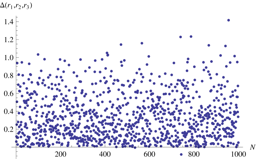
Figure 1: (Color online) Random testing of the violation of the triangular inequality for $\mathbf{D}_{\hat{J}}$ by using mixed qubit states. The horizontal axis $N$ represents the numbers of $\boldsymbol{\Delta}(\boldsymbol{r}_{1},\boldsymbol{r}_{2},\boldsymbol{r}_{3})$ which are calculated here. $\rho(\boldsymbol{r}_{1}),\rho(\boldsymbol{r}_{2})$ and $\rho(\boldsymbol{r}_{3})$ are generally not pure states. The points under the horizontal axis indicate the violation of the triangular inequality by triples of three qubit states.

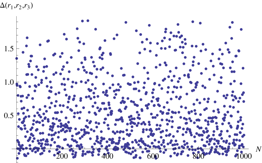
Figure 2: (Color online) Random testing of the violation of the triangular inequality for $\mathbf{D}_{\hat{J}}$ by using pure qubit states. The horizontal axis $N$ represents the numbers of $\boldsymbol{\Delta}(\boldsymbol{r}_{1},\boldsymbol{r}_{2},\boldsymbol{r}_{3})$ which are calculated here. All $\rho(\boldsymbol{r}_{1}),\rho(\boldsymbol{r}_{2})$ and $\rho(\boldsymbol{r}_{3})$ are pure states). The points under the horizontal axis indicate the violation of the triangular inequality by triples of three qubit pure states.

In FIG. 2, as suggested in this figure, the inequality $\boldsymbol{\Delta}\geqslant 0$, i.e., the triangle inequality, is violated by a lot of random samples representing pure qubit states. Again, $\mathbf{D}_{\hat{J}}$ is not the true metric over the set of all pure qubit states.

Figure 3: (Color online) Random testing of the violation of the triangular inequality for $\mathbf{D}^{2}_{\hat{J}}$ by using mixed qubit states. The horizontal axis $N$ represents the numbers of $\boldsymbol{\Delta}^{\prime}$ which are calculated here. $\rho_{1}=\rho(\boldsymbol{r}_{1}),\rho_{2}=\rho(\boldsymbol{r}_{2})$ and $\rho=\rho(\boldsymbol{r}_{3})$ are generally not pure states. The points under the horizontal axis indicate the violation of the triangular inequality by triples of three qubit states.

Figure 4: (Color online) Random testing of the violation of the triangular inequality for $\mathbf{D}^{2}_{\hat{J}}$ by using pure qubit states. The horizontal axis $N$ represents the numbers of $\boldsymbol{\Delta}^{\prime}$ which are calculated here. All $\rho_{1}=\rho(\boldsymbol{r}_{1}),\rho_{2}=\rho(\boldsymbol{r}_{2})$ and $\rho=\rho(\boldsymbol{r}_{3})$ are pure states). The points under the horizontal axis indicate the violation of the triangular inequality by triples of three qubit pure states.

Denote

$$\boldsymbol{\Delta}^{\prime} = \mathbf{D}^{2}_{\hat{J}}(\rho(\boldsymbol{r}_{1}),\rho(\boldsymbol{r}_{2}))+\mathbf{D}^{2}_{\hat{J}}(\rho(\boldsymbol{r}_{1}),\rho(\boldsymbol{r}_{3}))-\mathbf{D}^{2}_{\hat{J}}(\rho(\boldsymbol{r}_{2}),\rho(\boldsymbol{r}_{3})).$$

In FIG. 3 and FIG. 4, we demonstrate the fact that $\mathbf{D}^{2}_{\hat{J}}$ is still not the true metric when restricted to the set $\mathrm{D}\left(\mathbb{C}^{2}\right)$ and the set of all pure qubit states, respectively.

3.4 The spectral density of mixture under the so-called quantum addition rule

Assume that both $\rho_{1}$ and $\rho_{2}$ are i.i.d. random density matrices for qubits, chosen from respective unitary orbits $\mathcal{O}_{\mu}$ and $\mathcal{O}_{\nu}$ with $\mu,\nu$ are fixed in the open interval $(0,1/2)$. Denote $\rho(\hat{\boldsymbol{r}})=\rho(\boldsymbol{r}_{1})\boxplus_{1/2}\rho(\boldsymbol{r}_{2})$. Let $\hat{r}=\left\lvert\mspace{1.0mu}\hat{\boldsymbol{r}}\mspace{1.0mu}\right\rvert,r_{1}=\left\lvert\mspace{1.0mu}\boldsymbol{r}_{1}\mspace{1.0mu}\right\rvert$ and $r_{2}=\left\lvert\mspace{1.0mu}\boldsymbol{r}_{2}\mspace{1.0mu}\right\rvert$.

Theorem 3.7.

The conditional probability density of $\hat{r}$ with respect to fixed $r_{1},r_{2}$ is given by

$$q(\hat{r}|r_{1},r_{2})=\frac{1}{r_{1}r_{2}}\cdot\frac{2\hat{r}}{\sqrt{(1+r^{2}_{1})(1+r^{2}_{2})-4\hat{r}^{2}}},$$ (3.23)

where $\hat{r}\in[r_{-},r_{+}]$ with $r_{-}=\frac{\left\lvert\mspace{1.0mu}r_{1}-r_{2}\mspace{1.0mu}\right\rvert}{2}$ and $r_{+}=\frac{r_{1}+r_{2}}{2}$.

Proof.

As already noticed above,

$$\hat{r}=\frac{1}{2}\sqrt{r^{2}_{1}+r^{2}_{2}+2r_{1}r_{2}\cos\theta+r^{2}_{1}r^{2}_{2}\sin^{2}\theta}.$$

That is, $\hat{r}=\frac{1}{2}\sqrt{(1+r^{2}_{1})(1+r^{2}_{2})-(1-r_{1}r_{2}\cos\theta)^{2}}$. Since the probability density function of $\theta$ is given by $\frac{1}{2}\sin\theta\mathrm{d}\theta$, it follows that $\cos\theta,\theta\in[0,\pi]$ has the constant density $\frac{1}{2},\cos\theta\in[-1,1]$. By change of variables, we finally get the desired density $q(\widetilde{r}|r_{1},r_{2})$. ∎

From this theorem, we can infer the spectral density of the mixture of two random density matrices for qubits under the quantum addition rule: $\rho_{1}\boxplus_{1/2}\rho_{2}=\frac{1}{2}(\rho_{1}+\rho_{2}-\mathrm{i}[\rho_{1},\rho_{2}])$.

Corollary 3.8.

The spectral density of $\rho_{1}\boxplus_{1/2}\rho_{2}$, where $\rho_{1}$ and $\rho_{2}$ chosen uniformly from respective unitary orbits $\mathcal{O}_{\mu}$ and $\mathcal{O}_{\nu}$ with $\mu,\nu$ are fixed in the open interval $(0,1/2)$, is given by

$$q(\hat{\lambda}|\mu,\nu)=\frac{1}{2\left(\frac{1}{2}-\mu\right)\left(\frac{1}{2}-\nu\right)}\frac{\left\lvert\mspace{1.0mu}\hat{\lambda}-\frac{1}{2}\mspace{1.0mu}\right\rvert}{\sqrt{(2\mu^{2}-2\mu+1)(2\nu^{2}-2\nu+1)-\left(2\hat{\lambda}-1\right)^{2}}},$$

where $\hat{\lambda}\in[T_{0},T_{1}]\cup[1-T_{1},1-T_{0}]$. Note that $T_{0}$ and $T_{1}$ can be found in Proposition 3.1.

Proof.

The proof easily follows from Theorem 3.7. ∎

Here we give the figures to show how $p(\lambda|\mu,\nu)$ in Proposition 3.1 and $q(\hat{\lambda}|\mu,\nu)$ in Corolloary 3.8 change with $\lambda$ and $\hat{\lambda}$ when $\mu,\nu$ chosen, respectively, in FIG. 5; $p(r|r_{1},r_{2})$ in Theorem 3.2 and $q(\hat{r}|r_{1},r_{2})$ in Theorem 3.7 with $r$ and $\hat{r}$, respectively, in FIG. 6.

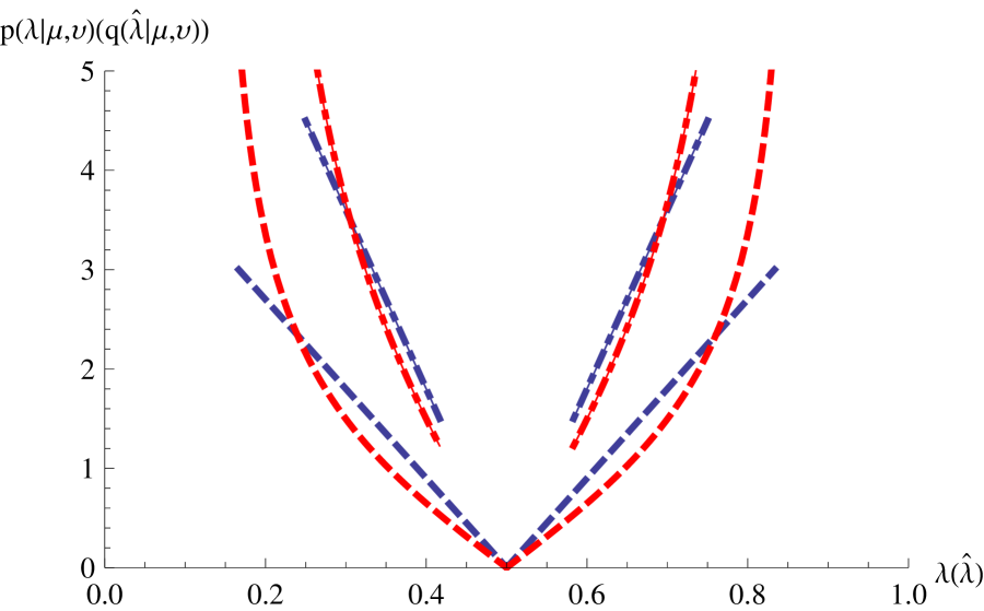
Figure 5: (Color online) The eigenvalue densities of two kinds of mixtures of two qubit states. $p(\lambda|\mu,\nu)$ in Proposition 3.1 versus $\lambda$ and $q(\hat{\lambda}|\mu,\nu)$ in Corollary 3.8 versus $\hat{\lambda}$: $p(\lambda|\mu,\nu)$ is represented by the blue line and $q(\hat{\lambda}|\mu,\nu)$ is represented by the red line. The solid line ($\mu=\frac{1}{3}$,$\nu=\frac{1}{6}$), the dashed line ($\mu=\nu=\frac{1}{6}$) and the dot-dashed line ($\mu=\frac{1}{6}$,$\nu=\frac{1}{3}$), both the solid line and the dot-dashed line are coincided.

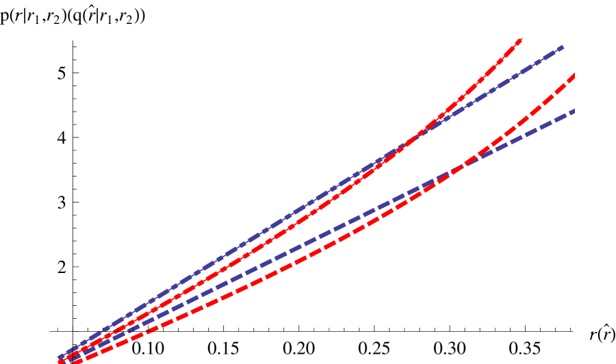
Figure 6: (Color online) The densities of the lengths of the Bloch vectors for two kinds of mixtures of two qubit states. $p(r|r_{1},r_{2})$ in Theorem 3.2 versus $r$ and $q(\hat{r}|r_{1},r_{2})$ in Theorem 3.7 versus $\hat{r}$: $p(r|r_{1},r_{2})$ is represented by the blue line and $q(\hat{r}|r_{1},r_{2})$ is represented by the red line. The solid line ($r_{1}=\frac{1}{3}$,$r_{2}=\frac{2}{3}$), the dashed line ($r_{1}=r_{2}=\frac{2}{3}$) and the dot-dashed line ($r_{1}=\frac{2}{3}$,$r_{2}=\frac{1}{3}$), both the solid line and the dot-dashed line are coincided.

4 Further observations

We have derived the spectral density of the equiprobable mixture of two random density matrices for qubits, whose density function is given by (3.1). We can use this to calculate the average entropy of the equiprobable mixture of two random density matrices for qubits. Let $\mu,\nu\in[0,1/2]$. Choose $\rho_{1}\in\mathcal{O}_{\mu}$ and $\rho_{2}\in\mathcal{O}_{\nu}$ according to the Haar measure over the unitary group $\mathrm{S}\mathrm{U}(2)$. The average entropy of the equiprobable mixture of two random density matrices is given by

$$\mathbb{E}_{(\rho_{1},\rho_{2})\in\mathcal{O}_{\mu}\times\mathcal{O}_{\nu}}\mathrm{S}\left(\frac{\rho_{1}+\rho_{2}}{2}\right)=\iint\mathrm{d}\mu_{\mathrm{Haar}}(U)\mathrm{d}\mu_{\mathrm{Haar}}(V)\mathrm{S}\left(\frac{U\rho_{1}U^{\dagger}+V\rho_{2}V^{\dagger}}{2}\right).$$

By using the result in Theorem 3.2, we get that

Proposition 4.1.

The average entropy of the equiprobable mixture of two random density matrices chosen uniformly from orbits $\mathcal{O}_{\mu}$ and $\mathcal{O}_{\nu}$, respectively, is given by the formula:

$$\int^{r_{+}}_{r_{-}}\Phi(r)p(r|r_{1},r_{2})\mathrm{d}r=\frac{2}{r_{1}r_{2}}\int^{r_{+}}_{r_{-}}\Phi(r)r\mathrm{d}r,$$ (4.1)

where $r_{+}:=\frac{r_{1}+r_{2}}{2},r_{-}:=\frac{\left\lvert\mspace{1.0mu}r_{1}-r_{2}\mspace{1.0mu}\right\rvert}{2}$ for $r_{1}=\frac{1-\mu}{2},r_{2}=\frac{1-\nu}{2}$, and $\Phi(x)=-\frac{1+x}{2}\log_{2}\frac{1+x}{2}-\frac{1-x}{2}\log_{2}\frac{1-x}{2}$.

Denote

$$\phi(x):=x^{2}(1+6\ln 2)+(1-x)^{2}(1+2x)\ln(1-x)+(1+x)^{2}(1-2x)\ln(1+x).$$

The average entropy is reduced to the following:

$$\frac{\phi(r_{+})-\phi(r_{-})}{6\ln 2\cdot r_{1}r_{2}}.$$

Furthermore, we can calculate the average entropy of the equiprobable mixture of two random states distributed according to the Hilbert-Schmidt measure over $\mathrm{D}\left(\mathbb{C}^{2}\right)$. Specifically, using the distribution densities of $r_{1}$ and $r_{2}$, we have

$$\mathbb{E}_{\rho_{1},\rho_{2}}\mathrm{S}\left(\frac{\rho_{1}+\rho_{2}}{2}\right)=18\int^{1}_{0}\int^{1}_{0}\mathrm{d}r_{1}\mathrm{d}r_{2}\left[r_{1}r_{2}\int^{r_{+}}_{r_{-}}\Phi(r)r\mathrm{d}r\right]\approx 0.7631.$$

Similarly, we can calculate the average entropy of the mixture of two random density matrices for qubits under the quantum addition rule: $\rho_{1}\boxplus_{1/2}\rho_{2}$, where $\rho_{1}\in\mathcal{O}_{\mu}$ and $\rho_{2}\in\mathcal{O}_{\nu}$. The average entropy of the mixture $\rho_{1}\boxplus_{1/2}\rho_{2}$ is given by

$$\mathbb{E}_{(\rho_{1},\rho_{2})\in\mathcal{O}_{\mu}\times\mathcal{O}_{\nu}}\mathrm{S}\left(\rho_{1}\boxplus_{1/2}\rho_{2}\right)=\iint\mathrm{d}\mu_{\mathrm{Haar}}(U)\mathrm{d}\mu_{\mathrm{Haar}}(V)\mathrm{S}\left(U\rho_{1}U^{\dagger}\boxplus_{1/2}V\rho_{2}V^{\dagger}\right).$$

By using the result in Theorem 3.7, we have that

Proposition 4.2.

According to the quantum addition rule, the average entropy of the mixture of two random density matrices chosen from orbits $\mathcal{O}_{\mu}$ and $\mathcal{O}_{\nu}$, respectively, is given by the formula:

$$\int^{r_{+}}_{r_{-}}\Phi(\hat{r})q(\hat{r}|r_{1},r_{2})\mathrm{d}\hat{r}=\frac{2}{r_{1}r_{2}}\int^{r_{+}}_{r_{-}}\frac{\Phi(\hat{r})\hat{r}\mathrm{d}\hat{r}}{\sqrt{(1+r^{2}_{1})(1+r^{2}_{2})-4\hat{r}^{2}}},$$ (4.2)

where $r_{+}:=\frac{r_{1}+r_{2}}{2},r_{-}:=\frac{\left\lvert\mspace{1.0mu}r_{1}-r_{2}\mspace{1.0mu}\right\rvert}{2}$ for $r_{1}=\frac{1-\mu}{2},r_{2}=\frac{1-\nu}{2}$, and $\Phi(x)=-\frac{1+x}{2}\log_{2}\frac{1+x}{2}-\frac{1-x}{2}\log_{2}\frac{1-x}{2}$.

Analogously, we can calculate the average entropy of the mixture under the quantum addition rule of two random states distributed according to the Hilbert-Schmidt measure over $\mathrm{D}\left(\mathbb{C}^{2}\right)$. Specifically,

$$\mathbb{E}_{\rho_{1},\rho_{2}}\mathrm{S}(\rho_{1}\boxplus_{1/2}\rho_{2})$$

$$=18\int^{1}_{0}\int^{1}_{0}\mathrm{d}r_{1}\mathrm{d}r_{2}\left[r_{1}r_{2}\int^{r_{+}}_{r_{-}}\frac{\Phi(\hat{r})\hat{r}\mathrm{d}\hat{r}}{\sqrt{(1+r^{2}_{1})(1+r^{2}_{2})-4\hat{r}^{2}}}\right]$$

$$\approx 0.7152.$$

Recall that if a quantum system of Hilbert space dimension $mn$ is in a random pure bipartite state, the average entropy of a subsystem of dimension $m\leqslant n$ should be given by the simple and elegant formula $H_{mn}-H_{n}-\frac{m-1}{2n}$, where $H_{k}:=\sum^{k}_{j=1}1/j$ is the $k$-th harmonic number. This is so-called Page’s average entropy formula [26] which is useful as a way of understanding the information in black hole radiation. Using Page’s formula, we see that

$$\frac{1}{3}<\mathbb{E}_{\rho_{1},\rho_{2}}\mathrm{S}(\rho_{1}\boxplus_{1/2}\rho_{2})<\mathbb{E}_{\rho_{1},\rho_{2}}\mathrm{S}\left(\frac{\rho_{1}+\rho_{2}}{2}\right)<1.$$

This indicates that our numerical calculations for $\mathbb{E}_{\rho_{1},\rho_{2}}\mathrm{S}(\rho_{1}\boxplus_{1/2}\rho_{2})\approx 0.7152$ and $\mathbb{E}_{\rho_{1},\rho_{2}}\mathrm{S}\left(\frac{\rho_{1}+\rho_{2}}{2}\right)\approx 0.7631$ are compatible with the above inequality. It is also reasonably to conjecture that there is a chain of strict inequalities:

$$\mathbb{E}_{\rho_{1},\rho_{2}}\mathrm{S}\left(\frac{\rho_{1}+\rho_{2}}{2}\right)<\mathbb{E}_{\rho_{1},\rho_{2},\rho_{3}}\mathrm{S}\left(\frac{\rho_{1}+\rho_{2}+\rho_{3}}{3}\right)<\cdots<\mathbb{E}_{\rho_{1},\ldots,\rho_{n}}\mathrm{S}\left(\frac{\rho_{1}+\cdots+\rho_{n}}{n}\right)<1.$$ (4.3)

Indeed, denote $\Gamma=\sum^{n}_{j=1}\rho_{j}$ where each $\rho_{j}$ is randomly chosen from Hilbert-Schmidt ensemble in a generic qubit system. Thus

$$\frac{\sum^{n}_{j=1}\rho_{j}}{n}=\frac{\Gamma}{n}=\frac{1}{n}\left(\sum^{n}_{j=1}\frac{\Gamma-\rho_{j}}{n-1}\right).$$

Then by the concavity of von Neumann entropy, we see that

$$\mathrm{S}\left(\frac{\sum^{n}_{j=1}\rho_{j}}{n}\right)\geqslant\frac{1}{n}\sum^{n}_{j=1}\mathrm{S}\left(\frac{\Gamma-\rho_{j}}{n-1}\right).$$

Because $\rho_{1},\ldots,\rho_{n}$ are independent and identically distribution (i.i.d.), we have that, for each $j=1,\ldots,n$

$$\mathbb{E}_{\rho_{1},\ldots,\rho_{n}}\mathrm{S}\left(\frac{\Gamma-\rho_{j}}{n-1}\right)=\cdots=\mathbb{E}_{\rho_{1},\ldots,\rho_{n-1}}\mathrm{S}\left(\frac{\sum^{n-1}_{j=1}\rho_{j}}{n-1}\right).$$

Therefore, we obtain that

$$\mathbb{E}_{\rho_{1},\ldots,\rho_{n}}\mathrm{S}\left(\frac{\sum^{n}_{j=1}\rho_{j}}{n}\right)\geqslant\mathbb{E}_{\rho_{1},\ldots,\rho_{n-1}}\mathrm{S}\left(\frac{\sum^{n-1}_{j=1}\rho_{j}}{n-1}\right).$$

The strict inequality needs to be determined. Now we can use this result and results obtained in [27] to explain that the quantum coherence [28] decreases statistically as the mixing times $n$ increasing in the equiprobable mixture of $n$ qubits. Recall that the quantum coherence can be quantified by many ways [28]. Here we take the coherence measure defined via the relative entropy, i.e., the so-called relative entropy of coherence. The mathematical definition of the relative entropy of coherence can be given as $C_{r}(\rho):=\mathrm{S}(\rho^{D})-\mathrm{S}(\rho)$, where $\rho^{D}$ is the diagonal part of the quantum state $\rho$ with respect to a prior fixed orthonormal basis. Denote $\overline{C}^{(n)}_{r}$ the average coherence of the equiprobable mixture of $n$ i.i.d. random quantum states from the Hilbert-Schmidt ensemble. By deriving the spectral density of the mixture of 3 qubits and some analytical computations, we show that $\overline{C}^{(3)}_{r}<\overline{C}^{(2)}_{r}$ [27]. Numerical experiments further show that for any integer $n>3$,

$$\overline{C}^{(n)}_{r}<\cdots<\overline{C}^{(3)}_{r}<\overline{C}^{(2)}_{r}.$$

Thus, in the qubit case, we find that the quantum coherence monotonously decreases statistically as the mixing times $n$. Moreover, we believe that the quantum coherence approaches zero when $n\to\infty$.

Finally, we remark here that results in the present paper can be used to compute exactly the average squared fidelity [29]. The fidelity between two qubit density matrices $\rho$ and $\sigma$ is defined by $\mathrm{F}(\rho,\sigma):=\operatorname{Tr}\left(\sqrt{\sqrt{\rho}\sigma\sqrt{\rho}}\right)$, then

$$\mathbb{E}_{\rho,\sigma}\mathrm{F}^{2}(\rho,\sigma)=\frac{1}{2}\left(1+\left(3\pi/16\right)^{2}\right).$$ (4.4)

Indeed, it is easily seen that, the squared fidelity for the qubit case is given by

$$\mathrm{F}^{2}(\rho,\sigma)=2\sqrt{\operatorname{det}(\rho)\operatorname{det}(\sigma)}+\operatorname{Tr}\left(\rho\sigma\right).$$

By using Bloch representations of $\rho=\rho(\boldsymbol{u})$ and $\sigma=\rho(\boldsymbol{v})$, we have that

$$\mathrm{F}^{2}(\rho(\boldsymbol{u}),\rho(\boldsymbol{v}))=\frac{1}{2}\left[1+\left\langle\boldsymbol{u},\boldsymbol{v}\right\rangle+\sqrt{(1-u^{2})(1-v^{2})}\right],$$

where $\left\lvert\mspace{1.0mu}\boldsymbol{u}\mspace{1.0mu}\right\rvert=u\in[0,1]$ and $\left\lvert\mspace{1.0mu}\boldsymbol{v}\mspace{1.0mu}\right\rvert=v\in[0,1]$. In the following, we calculate the average squared fidelity: Indeed, for $\boldsymbol{u}$ and $\boldsymbol{v}$, denote by $\theta\in[0,\pi]$ the angle between $\boldsymbol{u}$ and $\boldsymbol{v}$, their joint distribution density is given by

$$p(\boldsymbol{u},\boldsymbol{v})=p(u,v,\theta)=\frac{9}{2}u^{2}v^{2}\sin\theta,\quad\theta\in[0,\pi].$$

Thus direct calculation gives rise to the desired result.

$$\mathbb{E}_{\rho,\sigma}\mathrm{F}^{2}(\rho,\sigma) = \mathbb{E}_{\boldsymbol{u},\boldsymbol{v}}\mathrm{F}^{2}(\rho(\boldsymbol{u}),\rho(\boldsymbol{v}))$$

$$= \int\mathrm{F}^{2}(\rho(\boldsymbol{u}),\rho(\boldsymbol{v}))p(\boldsymbol{u},\boldsymbol{v})[\mathrm{d}\boldsymbol{u}][\mathrm{d}\boldsymbol{v}]$$

$$= \frac{1}{2}\left(1+\left(3\pi/16\right)^{2}\right).$$

5 Concluding remarks

In this paper, we work out the spectral densities of two kinds of mixtures, i.e., the equiprobable mixture and the mixture under the quantum addition rule, of two-level random density matrices chosen uniformly from the Haar-distributed unitary orbits, respectively. Before our work in the present paper, researchers always focus on the eigenvalue statistics for individual quantum state ensemble, and used frequently free probabilistic tools to make asymptotic analysis to get much information about some statistical quantities. Although the spectral analysis of superposition of random pure states were performed recently [18, 19], the topic about the spectral densities for the mixtures of random density matrices from two quantum state ensembles is rarely touched upon previously. Moreover, our methods in the present paper can be further used to derive the spectral densities of two kinds of mixtures: $w\rho_{1}+(1-w)\rho_{2}$ and $\rho_{1}\boxplus_{w}\rho_{2}$ for qubits, where $w\in[0,1]$. Finally, we leave some open questions here: (i) Can Proposition 3.5 be generalized to a general qudit system? (ii) We conjecture that $\mathrm{S}(\rho_{1}\boxplus_{w}\rho_{2})\leqslant\mathrm{S}\left(w\rho_{1}+(1-w)\rho_{2}\right)$ for any $w\in[0,1]$ and $\rho_{1},\rho_{2}\in\mathrm{D}\left(\mathbb{C}^{d}\right)$. We believe that our contribution in exact spectral analysis of the mixtures of random states will spur more new developments of applying RMT in quantum information theory.

Acknowledgments

LZ is truly grateful to the reviewer’s comments and suggestions on improving the manuscript. LZ acknowledges Huangjun Zhu for improving the quality of our manuscript. LZ is supported by Natural Science Foundation of Zhejiang Province (LY17A010027) and NSFC (Nos.11301124, 61771174), and also supported by the cross-disciplinary innovation team building project of Hangzhou Dianzi University. Both JW and ZC are also supported by NSFC (Nos.11401007,11571313).