On the implementation of the spherical collapse model for dark energy models

Abstract

In this work we review the theory of the spherical collapse model and critically analyse the aspects of the numerical implementation of its fundamental equations. By extending a recent work by [1], we show how different aspects, such as the initial integration time, the definition of constant infinity and the criterion for the extrapolation method (how close the inverse of the overdensity has to be to zero at the collapse time) can lead to an erroneous estimation (a few per mill error which translates to a few percent in the mass function) of the key quantity in the spherical collapse model: the linear critical overdensity $\delta_{\rm c}$, which plays a crucial role for the mass function of halos. We provide a better recipe to adopt in designing a code suitable to a generic smooth dark energy model and we compare our numerical results with analytic predictions for the EdS and the $\Lambda$CDM models. We further discuss the evolution of $\delta_{\rm c}$ for selected classes of dark energy models as a general test of the robustness of our implementation. We finally outline which modifications need to be taken into account to extend the code to more general classes of models, such as clustering dark energy models and non-minimally coupled models.

1 Introduction

Since the discovery of the accelerated expansion of the Universe [e.g. 2, 3], later confirmed by a plethora of other probes [e.g. 4, 5, 6, 7], much research in cosmology has been devoted to its theoretical explanation. While at the moment a complete physical understanding is lacking, a general concordance cosmological model has been designed. According to it, the Universe is spatially flat, its expansion is homogeneous in all directions and the main source of the gravitational potential is due to the cold dark matter (CDM) component, whose effects are, as for our understanding, only of gravitational origin. While CDM adds up to 28% of the total energy budget of the Universe and standard matter, dubbed generically baryons, amounts to about 5%, the rest (approximately 67%) is the fluid responsible for the accelerated expansion of the Universe [6]. In its simplest version, according to the concordance cosmological model, this is represented by the cosmological constant $\Lambda$, a fluid with equation of state $w_{\Lambda}=P_{\Lambda}/(\rho_{\Lambda}c^{2})=-1$ and constant throughout the cosmic time. This model is commonly referred to as $\Lambda$CDM model.

The $\Lambda$CDM cosmology is a simple yet very powerful model able to explain the wealth of data available. It relies on the symmetries of the Friedmann-Robertson-Walker metric and on General Relativity as the theory describing the gravitational interaction. Nevertheless, the $\Lambda$CDM model is affected by severe conceptual and theoretical problems [8, 9, 10, 11, 12, 13, 14]. On the large scales probed so far, the model is very successful, but the same cannot be said for small scales [15, 16], even if on such scales, gas physics becomes very important.

Lacking a conclusive evidence about the cosmological constant, other models have been investigated and they can be divided into two main groups. The first one still relies on General Relativity and includes the so-called dark energy (DE) models. These models are characterised by an equation of state which, in principle, can be an arbitrary function of time (with the condition $w<-1/3$ to achieve an accelerated expansion). The equation of state is therefore regarded as a free function depending on some parameters which will be fitted to data. The simplest and most used model is the CPL parametrization [17, 18] and the equation of state $w(a)$ is a linear function of the scale factor. These models can be easily studied and put on firm theoretical basis in the framework of the scalar fields. When doing this, it is then necessary to specify the form of the self-interacting potential $V(\phi)$. Our ignorance on the equation of state is then translated into our ignorance of the potential. We refer to [19] and references therein for a list and a comparison about the background properties of quintessence and $k$-essence models.
A second class describes the so-called modified gravity models where the Lagrangian for the gravitational sector is different from the General Relativistic one. Notable examples are Brans-Dicke theory [20, 21], Kinetic Gravity Braiding (KGB) [22, 23] and $f(R)$ models [24, 25, 26, 27, 28]. For recent reviews, we refer to [29, 30, 31, 32, 33, 34, 35, 36].
The majority of dark energy and modified gravity models can be seen as particular subclasses of the Horndeski models [37, 38, 39], which represent the most general models with second order equations of motion.

It is always possible to construct designer dark energy and modified gravity models where the background is, by construction, fully described by the equation of state [40, 41, 19]. When this is chosen to be $w=-1$, at the background level the models are identical to the $\Lambda$CDM model. To distinguish them, it is therefore necessary to study the evolution of perturbations, in particular on non-linear scales, such as clusters [42]. Their abundance is strictly related to the underlying cosmological model [43, 44, 45, 46, 47, 48] and has direct influence on weak lensing peak counts [49, 50, 51, 52]. In particular, it is sensitive to the normalization of the matter power spectrum $\sigma_{8}$ and the matter density parameter $\Omega_{\rm m}$ [53] and to the evolution of the dark energy equation of state [54, 55, 56, 57].

A simple, but very powerful tool to study the non-linear evolution of structures is the spherical collapse model. This analytic approach was introduced by [58, 59] and lately extended and improved by many authors [60, 61, 62, 63, 64, 65, 66, 67, 68, 69, 70]. More recent works took into account extensions to smooth [71, 72, 73, 74, 75, 76] and clustering dark energy models [68, 77, 78, 79, 80, 81, 82, 83, 84], non-minimally coupled models [85, 86], coupled dark energy models [78, 87, 88], time varying vacuum cosmologies [89], decaying dark matter with the cosmological constant [90] and [91, 92, 93] included the effects of baryons (studying the formation of primordial structures, equations are kept linear). [94] studied the effects of velocity diffusion and [95] those of viscosity. [96] used Birkhoff’s theorem to derive the equations of motion which were used to study models interpolating between the $\Lambda$CDM and the DGP. Other works studied the evolution of non-linear perturbations in modified gravity models, such as $f(R)$ [97, 98, 99, 100], Galileon [101, 102], symmetron [103] and chameleon models [104, 105, 106]. A parametrised spherical collapse model where effects of several screening mechanism are considered is studied in [107]. Finally, [108, 109] studied the spherical collapse model taking into consideration the effect of neutrinos and [110] the effects of primordial magnetic fields.

In the framework of the spherical collapse model, the collapsing object can be considered as a closed sub-universe since in General Relativity Birkhoff’s theorem holds. It has spherical symmetry and a uniform density profile (top-hat) and being overdense with respect to the background density, it decouples from the Hubble flow, slows down and reaches a maximum radius at the turn-around time and starts to collapse. Theoretically the perturbation collapses to a point while in reality an equilibrium situation is reached due to the conversion of the energy released during the collapsing process into random thermal motion. This is not explicitly present in the formalism and virialization has to be inserted a posteriori.

Many improvements to this simple scenario have been introduced: spherical symmetry has been relaxed in favour of an ellipsoidal one [111, 112, 113, 114, 115, 116]; shear, tidal interactions and rotations have also been used to make the collapse more realistic and to evaluate how this reflects on the mass function [117, 118, 119, 120, 121, 122, 123, 124, 125].

While the top-hat approximation is justified in General Relativity (an initial top-hat profile does not change in time), this is not true any more in modified gravity models, such as $f(R)$, where shell crossing develops [97].

The main quantity evaluated within this formalism is the linearly extrapolated overdensity $\delta_{\rm c}(z)$ at a given collapse redshift $z_{\rm c}$ which represents the value of the linear evolution of the overdensity $\delta$ of a perturbation that collapses at the time $z_{\rm c}$ when the full non-linear equation is solved. It is not a quantity directly observable, but it represents the main ingredient for the mass function which is, as said above, an important tool for cosmology.

When the collapse stops, the radius is formally null and as a direct consequence, the density diverges. As [1] pointed out recently, a crucial point is how the infinity, or more precisely the numerical infinity to describe the collapse, is defined. In this work we aim to extend the analysis of [1] and, focusing on models within the general relativistic framework, we critically review all the numerical aspects to correctly solve the equations of motion of the spherical collapse model. We will concentrate not only on the definition of numerical infinity, but also on how to properly define the initial integration time and how to better determine the initial conditions.

In section 2 we review the equations of the spherical collapse model for quintessence models and discuss in detail the analytic results for the EdS and the $\Lambda$CDM model, which will be used later on to validate our implementation. In section 3 we analyse the effects on $\delta_{\rm c}$ of the numerical infinity, of the initial time where the integration starts and on the explicit set of the equations adopted, namely a single equation for $\delta$ or the combined set of equations for $\delta$ and the divergence of the velocity perturbation $\theta$. In section 4 we detail an improved implementation of the initial conditions and compare our numerical findings with the analytic results presented in section 2. This comparison will allow us to assess the validity and the numerical stability of our implementation for models beyond the $\Lambda$CDM. We want to stress that, differently from [1], we do not know in general which value we can expect for $\delta_{\rm c}$ for a model with a generic equation of state $w$ or for a $\Lambda$CDM model when the tidal shear and rotation invariants are considered. Finally we discuss our findings in section 5 and outline our code in more detail in Appendix A.

2 Spherical collapse model

In this section we review the formalism of the spherical collapse model and introduce its main quantities. We will then focus on the analytic results for the EdS and the $\Lambda$CDM model and consider them as a validity test for the novel implementation described in detail in section 4.

We will follow two different approaches: the first one, based on the evolution of the overdensity $\delta$, has very general validity and it will be used to derive the differential equations for $\delta$ which can be applied to a generic dark energy model, provided the appropriate background Hubble factor $H(a)$ is used, and to arbitrary geometry, once a model for the tidal shear and rotation invariants is assumed; the second one is the original approach based on the evolution of the radius of the collapsing sphere and it is very useful to derive analytic results for the EdS and the $\Lambda$CDM model.

When using the hydrodynamic approach, we can start from the metric of the perturbed sub-universe

$$ds^{2}=-(1+2\phi)c^{2}dt^{2}+a(t)^{2}(1-2\phi)\delta_{ij}dx^{i}dx^{j}\;,$$ (2.1)

where $a(t)$ is the scale factor, $\delta_{ij}$ the Kronecker delta and $\phi=\Phi/c^{2}$ the dimensionless Bardeen potential. By assuming the stress-energy tensor of a perfect fluid

$$T^{\mu\nu}=(\rho+P/c^{2})u^{\mu}u^{\nu}+Pg^{\mu\nu}\;,$$ (2.2)

where $\rho$ is the density of the fluid, $P=w\rho c^{2}$ its pressure and $w$ its equation of state. The four-velocity is $u^{\mu}=dx^{\mu}/d\tau$, where $\tau$ is the proper time.

Defining the density perturbation $\delta=\delta\rho/\bar{\rho}$ with $\bar{\rho}$ the background density and $\boldsymbol{u}$ the three-dimensional comoving peculiar velocity and projecting the continuity equation $\nabla_{\mu}T^{\mu\nu}=0$ over the four-velocity $u_{\nu}$ and the projection operator $h_{\nu\alpha}=g_{\nu\alpha}+u_{\nu}u_{\alpha}$, we recover the continuity and the Euler equations for the fluid

$$\dot{\delta}+(1+w)(1+\delta)\vec{\nabla}\cdot\boldsymbol{u}= \;0\;,$$ (2.3)

$$\dot{\boldsymbol{u}}+2H\boldsymbol{u}+(\boldsymbol{u}\cdot\vec{\nabla})\boldsymbol{u}+\frac{1}{a^{2}}\vec{\nabla}\psi= \;0\;,$$ (2.4)

where $\psi$ is the peculiar gravitational potential which satisfies the following Poisson equation

$$\nabla^{2}\psi=4\pi G(1+3w)a^{2}\bar{\rho}\delta\;.$$ (2.5)

Spatial derivatives are taken with respect to the comoving coordinate $\boldsymbol{x}$ and a dot represents the derivative with respect to cosmic time. Note that in deriving these equations we already have assumed the standard "top-hat" profile for the density perturbations.

From now on we consider a pressure-less fluid, namely matter with $w=0$ and density parameter $\Omega_{\rm m}(t)$, and we combine the continuity, (the divergence of the) Euler and Poisson equation to obtain the full non-linear differential equation describing the evolution of the density perturbation $\delta$ [112, 72]:

$$\ddot{\delta}+2H\dot{\delta}-\frac{4}{3}\frac{\dot{\delta}^{2}}{1+\delta}-\frac{3}{2}H^{2}\Omega_{\rm m}(t)\delta(1+\delta)-(1+\delta)(\sigma^{2}-\omega^{2})=0\;,$$ (2.6)

with $\sigma^{2}=\sigma_{ij}\sigma^{ij}$ and $\omega^{2}=\omega_{ij}\omega^{ij}$ the shear and rotation tensors. Under the standard top-hat approximation, they arise in the following decomposition

$$\vec{\nabla}\cdot[(\boldsymbol{u}\cdot\vec{\nabla})\boldsymbol{u}]=\frac{1}{3}\theta^{2}+\sigma^{2}-\omega^{2}\;,$$ (2.7)

with $\theta=\vec{\nabla}\cdot\boldsymbol{u}$ and are defined as

$$\sigma_{ij} =\;\frac{1}{2}\left(\frac{\partial u^{j}}{\partial x^{i}}+\frac{\partial u^{i}}{\partial x^{j}}\right)-\frac{1}{3}\theta\delta_{ij}\;,$$ (2.8)

$$\omega_{ij} =\;\frac{1}{2}\left(\frac{\partial u^{j}}{\partial x^{i}}-\frac{\partial u^{i}}{\partial x^{j}}\right)\;.$$ (2.9)

To determine the initial conditions, we seek for an initial overdensity $\delta_{\rm ini}$ such that $\delta(a_{\rm c})\rightarrow\infty$, where $a_{\rm c}$ is the collapse scale factor. At early times, $\delta\ll 1$ and we can neglect the non-linear terms in Eq. 2.6 and assume a power-law for the linear evolution of $\delta$. This procedure will allow us to determine $\dot{\delta}_{\rm ini}$.

Having at hands the initial conditions, we can solve the linearised version of Eq. 2.6, whose value at $a_{\rm c}$ represents the linear overdensity $\delta_{\rm c}$.

It is more convenient to solve the equations of motion having as independent variable the scale factor, so for completeness and for clarity in the description of the algorithm, we report both the non-linear and linear differential equations:

$$\delta^{\prime\prime}+\left(2+\frac{H^{\prime}}{H}\right)\delta^{\prime}-\frac{4}{3}\frac{{\delta^{\prime}}^{2}}{1+\delta}-\frac{3}{2}\Omega_{\rm m}(a)\delta(1+\delta)-(1+\delta)(\tilde{\sigma}^{2}-\tilde{\omega}^{2})=0\;,$$ (2.10)

$$\delta^{\prime\prime}+\left(2+\frac{H^{\prime}}{H}\right)\delta^{\prime}-\frac{3}{2}\Omega_{\rm m}(a)\delta=0\;,$$ (2.11)

where a prime represents the derivative with respect to $\ln{a}$ and $\tilde{\sigma}=\sigma/H$ and $\tilde{\omega}=\omega/H$. This is what we will refer to as implementation A.

In a more general setup, we might not only have dark matter and baryons clustering, but also dark energy. In this case, we need to take into account also possible dark energy perturbations and the equations for $\delta_{\rm de}$ will depend on the effective sound speed $c_{\rm eff}^{2}\equiv\delta P_{\rm de}/(\delta\rho_{\rm de}c^{2})$. Going from a system of two first order equations (one for $\delta$ and one for $\theta=\nabla\cdot\boldsymbol{u}$) to a single second order equation will introduce time derivatives of $c_{\rm eff}^{2}$ and furthermore make the overall equation quite complicated. It is therefore easier, also from a numerical point of view since precise initial conditions can be given, to consider the two equations for $\delta$ and $\theta$ which, for clustering dark energy models, are [79, 126, 47, 127]

$$\delta^{\prime}_{\rm m}+(1+\delta_{\rm m})\tilde{\theta}_{\rm m}=0\;,$$ (2.12)

$$\delta_{\rm de}^{\prime}+3\left(c_{\rm eff}^{2}-w_{\rm de}\right)\delta_{\rm de}+\left[1+w_{\rm de}+\left(1+c_{\rm eff}^{2}\right)\delta_{\rm de}\right]\tilde{\theta}_{\rm de}=0\;,$$ (2.13)

$$\tilde{\theta}_{\rm m}^{\prime}+\left(2+\frac{H^{\prime}}{H}\right)\tilde{\theta}_{\rm m}+\frac{\tilde{\theta}_{\rm m}^{2}}{3}+(\tilde{\sigma}^{2}-\tilde{\omega}^{2})+\frac{3}{2}\left[\Omega_{\rm m}(a)\delta_{\rm m}+\left(1+3c_{\rm eff}^{2}\right)\Omega_{\rm de}(a)\delta_{\rm de}\right]=0\;,$$ (2.14)

$$\tilde{\theta}_{\rm de}^{\prime}+\left(2+\frac{H^{\prime}}{H}\right)\tilde{\theta}_{\rm de}+\frac{\tilde{\theta}_{\rm de}^{2}}{3}+\frac{3}{2}\left[\Omega_{\rm m}(a)\delta_{\rm m}+\left(1+3c_{\rm eff}^{2}\right)\Omega_{\rm de}(a)\delta_{\rm de}\right]=0\;,$$ (2.15)

where we assumed that dark energy is not affected by the $\tilde{\sigma}^{2}-\tilde{\omega}^{2}$ term. The corresponding linear equations are

$$\delta^{\prime}_{\rm m}+\tilde{\theta}_{\rm m}=0\;,$$ (2.16)

$$\delta_{\rm de}^{\prime}+3\left(c_{\rm eff}^{2}-w_{\rm de}\right)\delta_{\rm de}+(1+w_{\rm de})\tilde{\theta}_{\rm de}=0\;,$$ (2.17)

$$\tilde{\theta}_{\rm m}^{\prime}+\left(2+\frac{H^{\prime}}{H}\right)\tilde{\theta}_{\rm m}+\frac{3}{2}\left[\Omega_{\rm m}(a)\delta_{\rm m}+\left(1+3c_{\rm eff}^{2}\right)\Omega_{\rm de}(a)\delta_{\rm de}\right]=0\;,$$ (2.18)

$$\tilde{\theta}_{\rm de}^{\prime}+\left(2+\frac{H^{\prime}}{H}\right)\tilde{\theta}_{\rm de}+\frac{3}{2}\left[\Omega_{\rm m}(a)\delta_{\rm m}+\left(1+3c_{\rm eff}^{2}\right)\Omega_{\rm de}(a)\delta_{\rm de}\right]=0\;,$$ (2.19)

where $\tilde{\theta}=\theta/H$. Therefore at linear level $\tilde{\theta}_{\rm m}=\tilde{\theta}_{\rm de}$. This is what we will refer to as implementation B. Note that all the following discussion will be based on the assumption that dark energy is important only at the background level. We reported the full equations including dark energy perturbations for completeness and we will explain in section 5 what is necessary to be done to include them consistently.

Finally, as one may suspect and as [1] described at length, a crucial point of the previous approach is the definition of numerical infinity, which [1] can fix together with the initial conditions for the perturbations knowing the result at the collapse time. This is in general not the case when dealing with general dark energy models or also for EdS and $\Lambda$CDM models when the assumption of spherical symmetry is dropped, even if, in a realistic setting, the difference is at the percent level [123, 124]. As shown in these works, the problem of infinity can be avoided and a more numerically stable system of equations can be derived by noticing that while the density perturbation diverges, its inverse goes to zero. Therefore, defining $f\equiv 1/\delta$, our new system is now

$$f^{\prime}-f(1+f)\tilde{\theta}=0\;,$$ (2.20)

$$\tilde{\theta}^{\prime}+\left(2+\frac{H^{\prime}}{H}\right)\tilde{\theta}+\frac{\tilde{\theta}^{2}}{3}+\frac{3}{2}\frac{\Omega_{\rm m}(a)}{f}+(\tilde{\sigma}^{2}-\tilde{\omega}^{2})=0\;,$$ (2.21)

with corresponding linear equations

$$f^{\prime}-f^{2}\tilde{\theta}=0\;,$$ (2.22)

$$\tilde{\theta}^{\prime}+\left(2+\frac{H^{\prime}}{H}\right)\tilde{\theta}+\frac{3}{2}\frac{\Omega_{\rm m}(a)}{f}=0\;.$$ (2.23)

We will refer to this set of equations as implementation C.

To obtain analytic results for the EdS and the $\Lambda$CDM model, it is more convenient to use the formulation which follows the evolution of the radius of the sphere. From this point of view, the perturbation, characterised by a given constant mass $M$, starts with an initial radius $R_{\rm ini}$ at time $t_{\rm ini}$, evolves to reach a maximum value (turn-around radius $R_{\rm ta}$) and decreases to zero when the collapse is reached. In reality this does not happen, and the radius will reach a value, called virial radius $R_{\rm vir}$ due to the virialization process. Also in this case, virialization needs to be inserted a posteriori in the formalism. Attempts to embed the virialization process by modifying the equations of motion have been pursued by [128] and [129].

For the derivation of the following results, both at the collapse and at the virialization redshift, we closely follow [130, 131]. Since explicit analytic results can be obtained for the EdS model, but not in general for a $\Lambda$CDM model, here we will only report the EdS ones and refer to the aforementioned works for general expressions.

Let us then consider a universe characterised by matter, curvature and dark energy whose equation of state is $w_{\rm de}(a)$. Being interested to the late time evolution of the perturbations, we will neglect radiation. One can define the scale factor $x$ and radius $y$ of the perturbation normalised at turn-around:

$$x\equiv\frac{a}{a_{\rm ta}}\;,\quad y\equiv\frac{R}{R_{\rm ta}}\;,$$

where $R$ is the true radius of the sphere, $a_{\rm ta}$ and $R_{\rm ta}$ the turn-around scale factor and radius, respectively.

Denoting by $\omega$ and $\lambda$ the matter and dark energy density parameters at turn-around, respectively, the two Friedmann equations describing the collapse are

$$\dot{x} =\left[\frac{\omega}{x}+\lambda x^{2}g(x)+(1-\omega-\lambda)\right]^{1/2}\;,$$ (2.24)

$$\ddot{y} =-\frac{\omega\zeta_{\rm ta}}{2y^{2}}-\frac{1+3w(x)}{2}\lambda g(x)y\;,$$ (2.25)

where the dot represents the derivative with respect to the dimensionless time parameter $\tau\equiv H_{\rm ta}t$ and $g(x)$ the change in the dark energy density relative to turn-around,

$$g(x)=\exp{\left\{-3\int_{1}^{x}[1+w(x^{\prime})]\leavevmode\nobreak\ {\rm d}\ln{x^{\prime}}\right\}}\;.$$ (2.26)

Finally $\zeta_{\rm ta}$ represents the non-linear overdensity of the collapsing sphere with respect to the background at the turn-around.

For a constant dark energy equation of state $w_{\rm de}$ and flat spatial geometry, the solution of Eq. 2.24 is

$$\tau=\frac{2}{3\sqrt{\omega}}x^{3/2}{}_{2}F_{1}\left(\frac{1}{2},-\frac{1}{2w_{\rm de}};1-\frac{1}{2w_{\rm de}};-x^{-3w_{\rm de}}\frac{\lambda}{\omega}\right)\;,$$ (2.27)

where ${}_{2}F_{1}(a,b;c;z)$ is the hypergeometric function. This expression, for $w_{\rm de}=-1$, is identical to what was found by [96].

For an EdS model, the time of turn-around is therefore $\tau_{\rm ta}=2/3$ ($x_{\rm ta}=1$ by definition and ${}_{2}F_{1}(a,b;c;0)=1$). Since the collapse is symmetric around the turn-around, $t_{\rm c}=2t_{\rm ta}$, we can find the relation between the turn-around and the collapse: $a_{\rm ta}=(1/2)^{2/3}a_{\rm c}$.

The solution of Eq. 2.25 is quite complicate in general and albeit exact for a $\Lambda$CDM model, it is of little use because it can only be inverted numerically. We will therefore concentrate only on a dark energy model with $w_{\rm de}=-1/3$ and afterwards take the limit of $\omega=1$. When doing so, we obtain

$$\zeta_{\rm ta}=\left(\frac{3\pi}{4}\right)^{2}\left[{}_{2}F_{1}\left(\frac{1}{2},\frac{3}{2};\frac{5}{2};-\frac{\lambda}{\omega}\right)\right]^{-2}\;,$$ (2.28)

which, for $\omega=1$, gives $\zeta_{\rm ta}=\left(\tfrac{3\pi}{4}\right)^{2}\simeq 5.55$ [132].

Having this information at hand, we can now evaluate the two most important quantities of the spherical collapse model: the linearly extrapolated overdensity at the collapse, $\delta_{\rm c}$, and the virial overdensity $\Delta_{\rm V}$. We will also show how to evaluate these same quantities at the virialization redshift.

For an EdS model, the exact solution of Eq. 2.25 is [130, 131]

$$\tau=\frac{1}{\sqrt{\zeta_{\rm ta}}}\left[\frac{1}{2}\arcsin{(2y-1)}-\sqrt{y-y^{2}}+\frac{\pi}{4}\right]\;,$$ (2.29)

which at early times expands into

$$\tau\approx\frac{8}{9\pi}y^{3/2}\left[1+\frac{3}{10}y\right]\;.$$ (2.30)

The overdensity inside the perturbation with respect to the background is

$$\Delta=\left(\frac{x}{y}\right)^{3}\zeta_{\rm ta}\approx 1+\frac{3}{5}y\;,$$ (2.31)

where the approximation holds at early times. The linear density contrast inside the perturbation is $\delta=\Delta-1$. At turn-around we have $\delta_{\rm ta}=\frac{3}{5}\frac{y}{x}$ and $1/x\approx\left(\frac{3\pi}{4}\right)^{2/3}/y$ so that

$$\delta_{\rm ta}=\frac{3}{5}\left(\frac{3\pi}{4}\right)^{2/3}\simeq 1.06\;.$$

To determine the virial radius $y_{\rm vir}=R_{\rm vir}/R_{\rm ta}$ one can consider the virialization equation combining the classical virial theorem $T=-\frac{R}{2}\frac{\partial U}{\partial R}$, where $U$ is the potential energy associated with the overdensity, with the assumption that energy is conserved during the collapse. Despite this being a common assumption, for models beyond EdS it has not been proven whether it can actually be applied. For example, energy conservation is violated between turn-around and collapse when $w\neq-1,-1/3$ [133, 134, 135]. For an EdS universe, the solution of the equation

$$\left[U+\frac{\partial U}{\partial R}\right]_{\rm vir}=U_{\rm ta}\;,$$ (2.32)

leads to $y_{\rm vir}=1/2$. For $\Lambda$CDM and dynamical dark energy models a major result is by [136]:

$$y_{\rm vir}=\frac{1-\eta_{\rm v}/2}{2+\eta_{\rm t}-3\eta_{\rm v}/2}\;,$$ (2.33)

where

$$\eta_{\rm t}=2\zeta_{\rm ta}^{-1}\frac{\Omega_{\Lambda}(a_{\rm ta})}{\Omega_{\rm m}(a_{\rm ta})}\;,\quad\eta_{\rm v}=2\zeta_{\rm ta}^{-1}\left(\frac{a_{\rm ta}}{a_{\rm vir}}\right)^{3}\frac{\Omega_{\Lambda}(a_{\rm vir})}{\Omega_{\rm m}(a_{\rm vir})}\;.$$

These results can be obtained under the assumption that $y_{\rm vir}$ is only slightly different from the EdS value. The algebraic third order equation is then solved perturbatively.

For the virial overdensity, we cannot evolve the full non-linear equation up to the collapse redshift since, by definition, $\delta\rightarrow\infty$. We need therefore to use some recipe which allows us to define it. To do so, we use the recipe by [136] and [133]. Several recipes exist in the literature to evaluate the virial overdensity [64, 137, 138, 139, 140, 141, 133, 134]. We performed several tests using all of them and we noticed that they all agree, except for the recipe by [134] (they all agree for an EdS model). This difference was found also in the study of the relativistic virialization of structures [142]. In the following we will limit ourselves to the recipe of [136] and [133].

From the above definition for the non-linear overdensity $\Delta$, and considering the collapse taking place at $x_{\rm c}=2^{2/3}$, we find, for an EdS model,

$$\Delta_{\rm V}(a_{\rm c})=18\pi^{2}\simeq 177.65\;.$$

As pointed out by [130, 131], this is not entirely correct, as we should consider $x_{\rm vir}$, rather than $x_{\rm c}$. When $y_{\rm vir}=1/2$, $x_{\rm vir}=\left(\frac{3}{2}+\frac{1}{\pi}\right)^{2/3}$ and

$$\Delta_{\rm V}(a_{\rm vir})=18\pi^{2}\left(\frac{3}{4}+\frac{1}{2\pi}\right)^{2}\simeq 146.84\;.$$

In the limit $\tau\rightarrow 0$, $\Delta=1+\delta_{\rm lin}$, where [130, 131]

$$\delta_{\rm lin}=\frac{3}{5}\left(\frac{3}{2}\sqrt{\zeta_{\rm ta}}\tau\right)^{2/3}\;.$$ (2.34)

At the collapse

$$\delta_{\rm c}(a_{\rm c})=\frac{3}{20}(12\pi)^{2/3}\simeq 1.686\;,$$

while at the virialization

$$\delta_{\rm c}(a_{\rm vir})=\frac{3}{20}(6+9\pi)^{2/3}\simeq 1.58\;.$$

These values will be used to estimate the accuracy of the code.

In the following we will present numerical results only for the linearly evolved overdensity $\delta_{\rm c}$ and show results for the virial overdensity $\Delta_{\rm V}$ only for the optimised code, since this quantity is totally unaffected by numerical problems or the exact value of the initial conditions. For a more detailed analysis of why this is the case, we refer the reader to [123] in the more general analysis of the effect of the shear and rotation invariants.

3 Numerical analysis

In the following, we analyse different aspects of the spherical collapse model and show how the final result is affected by them. In subsection 3.1 we compare the three different formulations discussed in section 2. In subsection 3.2, as also done by [1], we show how different definitions of the value for the numerical infinity reflect on $\delta_{\rm c}$, while in subsection 3.3 we discuss the importance of setting correctly the initial integration time. Similarly, instead of considering implementations A and B, one could consider implementation C and investigate how close to zero the inverse of the density perturbation has to be to obtain stable and reliable results. This is discussed in subsection 3.4.

In this work, we will consider the following cosmological parameters: $\Omega_{\rm m}=0.3$, $\Omega_{\rm de}=0.7$ and $h=0.7$. Despite setting initial conditions at very early time, as it is commonly done in the studies of the spherical collapse model, we neglect the radiation contribution, setting $\Omega_{\rm r}=0$ throughout the cosmic history.

3.1 Dependence on the differential equation

To solve the three systems of equations, we need to fix some parameters, namely the numerical infinity $\delta_{\infty}$, the initial time $a_{\rm ini}$ where the integration starts and the numerical zero $f_{0}=1/\delta_{\infty}$. The differential equations are solved searching for the initial values of $\delta$ ($\delta^{\prime}$), $\theta$ and $f$ such that the collapse happens at a time specified in input. We consider as standard solver a Runge-Kutta Cash-Karp (4, 5) method as implemented in the publicly available library GSL. We refer the reader to section 4 for a more detailed discussion about the different choices used to evolve the perturbation equations.
Here we choose $a_{\rm ini}=10^{-5}$ for all the different implementations, $\delta_{\infty}=10^{8}$ and $f_{0}=10^{-8}$ as a result of the discussion which will follow in the next sections.

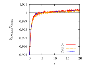
Figure 1: Ratio of $\delta_{c}$ between $\Lambda$CDM and EdS models as a function of the redshift $z$ for three different implementations. The red solid curve represents the solution of implementation A (a single second order differential equation), the orange dashed curve the solution of implementation B (two first order differential equations, one for $\delta$ and one for $\theta$), while the blue short-dashed curve represents the solution of implementation C (two first order differential equations, one for $f=1/\delta$ and one for $\theta$). The black solid line represents the exact asymptotic value that the ratio should reach.

In Fig. 1 we show the evolution of the ratio of $\delta_{\rm c}$ between a $\Lambda$CDM and an EdS model for the three different implementations discussed before. As it appears immediately clearly, on average, the solution is the same for all of them, as expected. In more detail, we see some substantial difference: implementations A and B are numerically noisier than implementation C. This is due to the fact that in general, the code hits the infinity barrier at slightly different values at each collapse redshift and the initial overdensity $\delta_{\rm ini}$ is affected by this. The blue dotted curve instead, is much smoother because it is easier to force the code, within a given accuracy, to reach $f_{0}$. From the point of view of numerical accuracy, implementation C is therefore numerically more stable.

Nevertheless, all three solutions show a similar trend which becomes relevant only at high redshifts though (differently from [82] where this was a substantial effect also at lower redshifts): despite approaching the EdS solution, $\delta_{\rm c}$ keeps growing and this would have important consequences on the mass function of high redshifts objects, with the result of predicting fewer objects. We also point out that at such high redshifts ($z\gtrsim 8$) an appropriate mass function must be used [see e.g. 143, for an in-depth discussion].

This is due to the fact that moving towards higher redshifts, $\delta_{\rm ini}$ grows too fast with respect to what is required (see Figure 8), because of small imprecisions arising from the combined effect of the root-finding algorithm, of the effective value of collapse $\delta_{\infty}$ ($1/\delta_{\infty}$) and of how the initial conditions are defined. Either solving a second order differential equation or a system of two differential equations, we require two initial conditions: for implementation A we need to find $\delta_{\rm ini}$ and $\delta_{\rm ini}^{\prime}$ while for implementation B we need $\delta_{\rm ini}$ and $\theta_{\rm ini}$ and for implementation C $f_{\rm ini}$ and $\theta_{\rm ini}$. Once $\delta_{\rm ini}$ or $f_{\rm ini}$ are found, $\delta_{\rm ini}^{\prime}$ and $\theta_{\rm ini}$ are related to them either via differentiation or via the continuity equation. Hence it is clear that a not exquisitely accurate determination of $\delta_{\rm ini}$ will have appreciable consequences.

Note however that the difference from a constant value is at the sub-percent level and of the order of 1-2% at most for $z\simeq 40$, making therefore results in literature generally correct.

As we will explain later in detail, this side effect can be avoided to a very high degree by refining the determination of the initial conditions.

3.2 Dependence on the collapse value

[1] pointed out clearly that results for $\delta_{\rm c}$ for a $f(R)$ model depend on the chosen value of the numerical infinity adopted and it is not correct to keep it constant when exploring the collapse at higher redshifts. The authors considered two different values for the collapse today: $\widetilde{\rm Inf}=10^{5}$ and $\widetilde{\rm Inf}=10^{8}$ setting the initial conditions at $z_{\rm ini}=1000$ and showed that this value can be as low as $10^{4}$ at collapse redshift $z\sim 3$ and that differences between the standard method and the method presented by the authors (based on the fact that they know what $\delta_{\rm c}$ should be at $z_{\rm c}=0$) grow increasing the redshift, since $\delta_{\rm c}$ grows without bound, as clearly shown in Fig. 1.

We want to investigate further the dependence of $\delta_{\rm c}$ on the exact value of the numerical infinity. The question we want to answer is: when can we be confident that the code converged, i.e., that when increasing the numerical infinity, the result does not change appreciably? We show this in Fig. 2, where we considered values of $\delta_{\infty}$ ranging from $10^{5}$ to $10^{9}$ for implementation B. Note also that this value is fixed and it does not change at higher collapse redshifts.

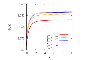
Figure 2: Critical collapse density $\delta_{\rm c}$ as a function of $z$ for different values of $\delta_{\infty}$. From bottom to top we consider: $10^{5}$ (red solid line), $10^{6}$ (orange dashed line), $10^{7}$ (blue short-dashed line), $10^{8}$ (brown dotted curve) and $10^{9}$ (grey dot-dashed curve), respectively.

It is clear that $\delta_{\rm c}$ depends critically on $\delta_{\infty}$. For a value as low as $\delta_{\infty}=10^{5}$, the value for $\delta_{\rm c}$ is substantially lower than the value expected, with a difference of about 2‰. This is roughly in agreement with what was found by [1]. Note that even if the difference might seem irrelevant and probably it is now with current data, it is not at all marginal for the mass function and the halo number counts for precision studies aiming to infer dark energy properties. Since at high mass, where we expect dark energy and modified gravity to play a considerable role, the mass function depends exponentially on the value of $\delta_{\rm c}$ and sub-percent differences here translate in differences of several percent in the mass function and quantities based on it, such as the Sunyaev-Zel’dovich (SZ) power spectrum. The evolution of $\delta_{\rm c}$ depends also on the physics considered, such as shear and rotation, or different gravitational models and it is therefore essential to have a converged result.

Increasing $\delta_{\infty}$ results in an increase of $\delta_{\rm c}$, such that for values of $\delta_{\infty}\geq 10^{7}$, the numerical solution has essentially converged to the expected value. Note that in Fig. 2 it is still possible to appreciate differences between $\delta_{\infty}=10^{7}$ and $\delta_{\infty}=10^{8}$, while for higher values differences are less than one part in $10^{4}$, approximately constant over all the redshifts investigated. We will hence consider from now on $\delta_{\infty}=10^{8}$.

Note that here, for clarity purposes, we smoothed the curves to suppress the numerical noise, so to be able to distinguish results for $\delta_{\infty}\geq 10^{7}$.

3.3 Dependence on the Time of the Initial Conditions

Another important quantity deserving attention is the time $a_{\rm ini}$ (or equivalently $z_{\rm ini}$), when initial conditions are set. Setting them too early will unnecessarily slow down the code, unless adaptive step-sizes are used, since we expect an EdS behaviour at high redshifts, unless early dark energy models are considered [144, 145, 146, 147, 148, 149, 150, 151]. On the other hand, setting them too late might not lead the code to the expected solution. This is because formally perturbations originate when $a_{\rm ini}\simeq 0$.

Here we recall how initial conditions are determined. The particular implementation is totally irrelevant, so we will just outline the general procedure. For a given collapse time $a_{\rm c}$, we need to infer the value of the initial overdensity $\delta_{\rm ini}$ such that $\delta(a_{\rm c})\rightarrow\infty$ or $f(a_{\rm c})\rightarrow 0$. In principle, $\delta_{\rm ini}$ can be specified as an input parameter, but this will lead to a collapse time that in general does not coincide with the desired one. The differential equation for $\delta_{\rm c}$ is then evolved having $\delta_{\rm ini}$ as initial condition.

In Fig. 3 we show the influence of the choice of $a_{\rm ini}$ on the evolution of the linearly extrapolated overdensity $\delta_{\rm c}$, as a function of redshift. Once again we consider a $\Lambda$CDM model. A similar behaviour happens in an EdS model. We present results for implementation C to have a smoother outcome, but we checked that a very similar result is found when considering the equations for $\delta$.

It is clear that to achieve a reliable result requires also an early time to start integrating the differential equations. We investigated different cases, ranging from $a_{\rm ini}=10^{-3}$ to $a_{\rm ini}=10^{-5}$. For large values of $a_{\rm ini}$, the numerical solution has certainly not converged since the perturbation did not collapse yet and as a consequence $\delta_{\rm c}$ grows unboundedly. We can observe a clear flattening of the curves decreasing the initial integration time. For $a_{\rm ini}$ as small as $10^{-5}$, the solution has definitely converged to the expected value (shown by the black solid line for the EdS model).

It is worth to investigate this aspect more in detail. [1] set their initial conditions at $z_{\rm ini}=10^{3}$ and find a reasonable solution for $\delta_{\rm c}$, for both $\delta_{\infty}=10^{5}$ and $10^{8}$, albeit not converging to the expected EdS solution (it grows unboundedly). [82], in the context of clustering early dark energy models, showed the evolution of $\delta_{\rm c}$ for a $\Lambda$CDM model. It converges to the numerical solution for an EdS cosmology for $z\simeq 4-5$, but both of them do not flatten to the expected analytic value. Nevertheless, their result is, within at most few percent, in agreement with what one has to expect. When instead we fix the value of $\delta$ (its inverse) to high (small) values, we find indeed an acceptable solution only for small enough $a_{\rm ini}$.

This result can be explained taking into account the settings of the different codes and the results of Fig. 2. We keep both $\delta_{\infty}$ and $a_{\rm ini}$ fixed and we do not change the first as a function of the collapsing time. The initial overdensity increases monotonically increasing the collapse redshift, but we do not have any scaling of our initial density perturbations since, for a generic dark energy model, we do not know a priori what the value for $\delta_{\rm c}$ should be, even if for a realistic model, it can not be too different from the $\Lambda$CDM value. This explains our findings with respect to [1]. When instead comparing our implementation with [82], we can appreciate the interplay and the degeneracy of $\delta_{\infty}$ and $a_{\rm ini}$. The authors fix the initial conditions at $z_{\rm ini}=10^{3}$ and assume $\delta_{\infty}=10^{5}$. According to our analysis, the first condition gives a too high value for $\delta_{\rm c}$, but a too low value for the latter. Both effects partially cancel each other delivering a good value for the linearly extrapolated overdensity. At the same time we notice that the sharp rise of $\delta_{\rm c}$ (our red solid line in Fig. 3) is only partially mitigated by a low value of $\delta_{\infty}$ in Fig. 7 of [82], being somehow intermediate with respect to our curves for $a_{\rm ini}=10^{-3}$ and $a_{\rm ini}=10^{-4}$.

This is a strong indication that not only the initial conditions have to be determined exquisitely well, but also all the other parameters can play a very important role if an analytic solution is not known. We will return to this point in section 4, where we discuss an alternative way to evaluate the initial conditions by scaling $a_{\rm ini}$.

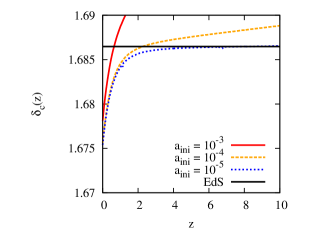
Figure 3: Evolution of $\delta_{\rm c}$ as a function of $z$ for a $\Lambda$CDM model for different values of $a_{\rm ini}$. The horizontal black solid curve represents the exact value of an EdS universe, the red solid curve the solution for $a_{\rm ini}=10^{-3}$, the orange (blue) dashed (short-dashed) curve the value for $a_{\rm ini}=10^{-4}$ ($a_{\rm ini}=10^{-5}$), respectively.

3.4 Dependence on the extrapolation

In Fig. 1 we showed that evolving the equation describing the evolution of $f=1/\delta$ gives a much less noisy result. While for the evolution of $\delta$ is critical to use a high enough value of $\delta_{\infty}$ for a proper numerical convergence to the analytic result, for $1/\delta$ it is important to know how close one has to be to zero to obtain the right answer. This is what we will discuss in this section. In the following we will consider, following the discussion in the previous section, $a_{\rm ini}=10^{-5}$.

While numerically it is difficult to compare two big numbers, it is much easier to compare two small numbers within a given precision range. Evolving $f=1/\delta$ implies as collapse condition that $f\rightarrow 0$. This cannot be achieved exactly but we can enforce it in this way: we evolve the system of differential equations till the collapse scale factor and till $f>\varepsilon=f_{0}$, but in general none of this conditions will be achieved exactly. The solver returns the value of $f$ and its derivative and we use this information to linearly extrapolate the value of $f$ to the exact collapse scale factor. In this way our solution is much less affected by the numerical noise due to the fact that the collapse condition and the collapse time are now reached exactly (within machine precision).

It is therefore important to determine how small $\varepsilon$ must be to achieve convergence of the result. We show the results of our analysis in Fig. 4.

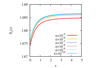
Figure 4: Evolution of $\delta_{\rm c}$ as a function of $z$ for a $\Lambda$CDM universe for different values of the extrapolation parameter $\varepsilon$. From bottom to top: the red (cyan) solid curve represents the solution for $\varepsilon=10^{-5}$ ($\varepsilon=10^{-10}$), the orange dashed curve $\varepsilon=10^{-6}$, the blue short-dashed curve $\varepsilon=10^{-7}$ and the brown dotted (grey dot-dashed) the solution for $\varepsilon=10^{-8}$ ($\varepsilon=10^{-9}$), respectively.

The situation is very similar to what was found and discussed before for $\delta_{\infty}$. When $\varepsilon=10^{-5}$, the perturbation is not collapsed yet and $\delta_{\rm c}$ is smaller than what it should be. This is in agreement with the results presented in Fig. 2: when $\delta_{\infty}=10^{5}$, the perturbation has not collapsed yet and the numerical value of $\delta_{\rm c}$ is smaller than the true one. The main difference is that the error now is smaller than before. Decreasing the value of $\varepsilon$ brings the numerical solution closer to the true one, so that, as expected from the discussion above, for $\varepsilon\leqslant 10^{-8}$, the numerical solution has completely converged to the true value. In the next section we will therefore assume $\varepsilon=10^{-8}$.

4 Improved Initial Conditions

After the discussion in section 3, we can now use the main results obtained to implement the equations of motion describing the evolution of the perturbations in an improved code. After discussing the details of the determination of the improved initial conditions and the structure of the code, we compare our numerical results with the analytic ones. According to the previous analysis, in the following we will consider the following parameters: $\delta_{\infty}=10^{8}$, $\varepsilon=10^{-8}$ and the maximum value to start integrating the equations $a_{\rm ini}=10^{-5}$.

As already discussed in detail in section 3, fixed initial conditions as well as a fixed value of numerical infinity lead to an artificial dependence of $\delta_{\rm c}$ on the chosen value of the collapse redshift. In the EdS limit, this leads to a small linear increase of the overdensity $\delta_{\rm c}$ with collapse redshift. [1] proposed a method to obtain the required value of the numerical infinity $\widetilde{\mathrm{Inf}}$ as a function of $z_{\rm c}$. This method requires calibrating the initial density contrast using the analytical results for the linear overdensity $\delta_{\rm c}$ in the EdS model where $\widetilde{\mathrm{Inf}}$ is assumed to be roughly independent of the cosmological model. We decided to use an alternative approach based on the appropriate rescaling of the initial scale factor to approximately match a constant value of the numerical infinity. As discussed in the previous section, the nonlinear evolution is described by the reciprocal density contrast $f$ and we therefore fix a lower bound $\epsilon$ to this quantity. The initial density contrast is then obtained by extrapolating $f_{\rm nl}$ to zero leading to the given initial value $f_{\rm ini}=1/\delta_{\rm ini}$. Since this procedure generically causes the value for the numerical infinity to depend on the collapse redshift, we need to change the initial conditions or equivalently the range of integration of the differential equation system to compensate for that. It turns out that an appropriate scaling for the initial scale factor is given by the linear growth factor of the model evaluated at the collapse scale factor. We therefore apply a simple rescaling law

$$a_{\rm ini}\longrightarrow\frac{a_{\rm ini}}{D_{+}(a_{\rm c})}\;.$$

By truncating the range of integration at a certain $a_{\rm c}<1$, the logarithmic range of numerical integration decreases by the amount $\sim-\log(D_{+}(a_{\rm c}))$ once the initial scale factor is fixed. Using this rescaling law, we keep the logarithmic size of integration interval approximately constant in $\log(a)$. Once the initial scale factor is rescaled, a constant value of numerical infinity is approximately matched. In case of the EdS model, the time evolution of $f$ is independent of the scale factor $a_{\rm c}$ and therefore a constant value of numerical infinity is matched exactly. In case of more complicated background fluids, this holds only approximately as the functional form of $f(a)$ changes with collapse redshift. We therefore rescale the initial scale factor by $D_{+}(a_{\rm c})$ instead of $a_{\rm c}$. Despite of that, this method does not require any calibration from an analytical result. Once this rescaling of the initial conditions is applied, results are perfectly stable up to collapse redshift of $20$ (the maximum we investigated) and reproduce the correct EdS value for $\delta_{\rm c}$ without initial calibration.

The following step is a further polishing of the initial conditions via a Newton-Raphson method. For the sake of computation time, we limit the code to five iterations. Starting from the initial guess of $\delta_{\rm ini}$, we evaluate the nonlinear value of $f$ and $\partial f/\partial\delta_{\rm ini}$ at the collapse and we move $\delta_{\rm ini}$ along the slope of the curve given by $f/(\partial f/\partial\delta_{\rm ini})$. If the change is smaller than about 10%, we stop the refinement.

In Fig. 5 we show the evolution of $\delta_{\rm c}$ for the two different initial conditions for a $\Lambda$CDM model. We consider implementation C for the old and new determination of the initial conditions. It is immediately clear that the improved initial conditions greatly improve the result. First of all the residual numerical noise due to the not exact estimation of the initial conditions is removed (for implementation A the numerical noise will be higher, but the time dependence identical). The initial overdensity is now accurate at the machine level thanks to the polishing procedure. In addition, and more importantly, $\delta_{\rm c}$ is now bounded: it reaches the theoretical value for an EdS model exactly and does not grow indefinitely, differently from before. This is a very important achievement showing the power of the new implementation. As a practical consequence, numerical values for $\delta_{\rm c}$ can now be used for the study of objects at high redshifts also with the help of the mass function, as discussed by [152].

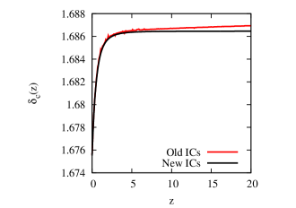
Figure 5: Comparison of $\delta_{\rm c}$ for different choices of initial conditions. The black (red noisy) solid curve represents the $\Lambda$CDM model with the novel (old) determination of the initial conditions. In both cases we used implementation C.

Having established the reliability of our code, we can now study in more detail some other quantities characterising the spherical collapse model. Apart from the value of $\delta_{\rm c}$ at the collapse, we can also study its evolution at the virialization redshift. While $\delta_{\rm c}$ represents the linear evolution of $\delta$, we can also investigate its non linear evolution, namely the virial overdensity $\Delta_{\rm V}$ at both the collapse and the virialization redshifts.

Since the collapse proceeds at a faster pace approaching the collapse time and the divergence appears formally only at the collapse, it is safe to integrate the full non-linear equation for $\delta$ till the virialization time. We verified that doing this is in excellent agreement with applying the recipe of [136] replacing all the quantities evaluated at collapse with the corresponding ones at the virialization.

To evaluate the turn-around scale factor $a_{\rm ta}$, we solve Eqs. 2.20 and 2.21 and determine $\log[(\delta_{\rm nl}+1)/a^{3}]$, which, besides irrelevant constants, is the inverse of the sphere radius $y$. The maximum value of $y$ is reached at the turn-around, therefore its inverse will reach at the same time its minimum. Hence, finding the location of the minimum will automatically give the value of the turn-around. Integrating the same set of equations till the turn-around will return $\zeta_{\rm ta}-1$.

Finally, the last quantity to evaluate is the virial scale factor $a_{\rm v}$. To do so, we first choose a recipe for the virialization process among the works cited above which provides the quantity $y_{\rm vir}$, then we look for the scale factor $x_{\rm v}=a_{\rm v}/a_{\rm ta}$ which minimises the function $\sqrt[3]{\zeta_{\rm ta}/(1+\delta_{\rm nl})}x_{\rm v}-r$. When this function is null with a precision of $10^{-8}$, the code returns the guessed value of $a_{\rm v}$. We repeat this procedure till the estimated virial scale factor does not change more than one part in $10^{8}$.

Later on we will compare the turn-around time $a_{\rm ta}$ and the non-linear overdensity $\zeta_{\rm ta}$ with theoretical predictions.

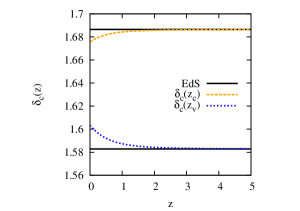
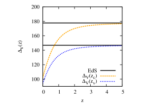
Figure 6: Left (right) panel: Evolution of $\delta_{\rm c}$ ($\Delta_{\rm V}$) evaluated at collapse $z_{\rm c}$ and virialization $z_{\rm v}$ redshift, respectively. The two horizontal black solid lines represent the EdS model, while the orange dashed and blue short-dashed lines the $\Lambda$CDM model. Upper (lower) curves show quantities at collapse (virialization) redshift.

In Fig. 6 we show the time evolution of $\delta_{\rm c}$ (left panel) and $\Delta_{\rm V}=\zeta_{\rm ta}\Omega_{\rm m}(a_{\rm c,v})(x/y)^{3}$ (right panel) as a function of the collapse ($a_{\rm c}$) or virialization ($a_{\rm v}$) scale factor for the EdS and $\Lambda$CDM models. It is clear that now the linear overdensity reaches exactly the theoretical value of an EdS model and does not grow further. This holds for both the EdS and the $\Lambda$CDM model, either at collapse or virialization. While the right panel does not reveal any surprise (the virial overdensity is smaller at late times where the cosmological constant dominates and approaches the EdS value for $z\gtrsim 5$), the left panel presents an interesting result. The upper curves show the linear overdensity at the collapse: at early times the two models give the same results as the EdS model is an excellent approximation, but at low redshift we have a different situation. When we consider the collapse time, the linear overdensity for the $\Lambda$CDM model is smaller than for an EdS model: this can be easily explained by taking into account that it is necessary to have a lower threshold for collapse because of the presence of the cosmological constant (analogous results are for generic dark energy models). When instead we consider the time of virialization, the expected value for $\delta_{\rm c}$ is higher for a $\Lambda$CDM than for an EdS one, while naively one could have thought the opposite behaviour, in analogy to the collapse. To explain this, it is useful to recall that $\delta_{\rm c}$ enters in the determination of the mass function: the number of massive objects must be the same both at the time of collapse and of virialization, since we consider a collapsed object virialized and vice versa. Hence one should not focus on $\delta_{\rm c}$ itself, but on the quantity $\nu_{\rm c}=\delta_{\rm c}(a_{\rm c})/D_{+}(a_{\rm c})$ which enters into the mass function. In the definition of $\nu_{\rm c}$, $D_{+}$ represents the linear growth factor. We checked that $\nu_{\rm c}=\nu_{\rm v}$ thus explaining the result in the left panel of Fig. 6. In other words, $\nu$ is a measure of $\delta_{\rm ini}$. We also compared our numerical solution with the fit provided by [96] for a flat $\Lambda$CDM model with $\Omega_{\rm m}=0.25$. For $0<z<5$, we found an agreement of the order 0.2%-0.3%.

In Fig. 7 we show the turn-around (left panel) and the corresponding value of the density $\zeta_{\rm ta}$ (right panel), again for an EdS and a $\Lambda$CDM model. Remember that, as explained before, the turn-around scale factor has been evaluated as the time when the normalised radius reaches unity. For these two models (but not for generic dark energy models), one could determine it as the half time of the collapse process. While this is correct, we saw that it leads to numerical noise in $\zeta_{\rm ta}$, therefore we prefer not to consider the symmetries of the models. The turn-around is identical for both models for $z\gtrsim 2$, while for $\zeta_{\rm ta}$ this is the case at higher redshifts ($z\gtrsim 5$). Requiring higher initial overdensity to overcome a faster expansion, for a $\Lambda$CDM model $\zeta_{\rm ta}$ is higher than for an EdS model and this reflects in an earlier turn-around. We checked that the numerical solution for an EdS model agrees with the theoretical prediction.

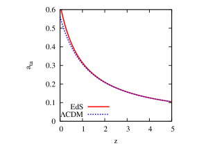
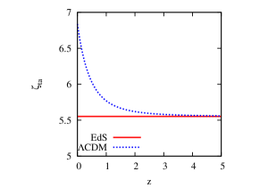
Figure 7: Left panel: evolution of the turn-around scale factor $a_{\rm ta}$ as a function of the collapse redshift. Right panel: evolution of the non-linear density $\zeta_{\rm ta}$ at turn-around. The solid red line shows the result for the EdS model, the dashed blue line for the $\Lambda$CDM result.

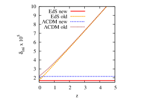
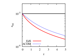
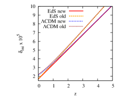
Figure 8: Top left panel: Evolution of the initial density perturbation $\delta_{\rm ini}$. The red solid (orange dashed) curve represents the values for an EdS model for the new (old) approach; the blue short-dashed and the brown dotted lines show the initial overdensity for a $\Lambda$CDM model for the new and the old implementation, respectively. Top right panel: Evolution of the initial scale factor $a_{\rm ini}$ where the integration starts. The solid red curve is for the EdS model while the blue dashed one stands for the $\Lambda$CDM model. The solid line at $a=10^{-5}$ reflects the old implementation. Bottom panel: evolution of $\delta_{\rm ini}$ in the old and in the new implementation, evolving it from $a_{\rm ini}$ to $a=10^{-5}$. Line styles and colours are as in the top panel.

Since the main difference between the old and the new implementation relies on a better estimation of the initial conditions, in Fig. 8 we show a comparison between the old and the new value of $\delta_{\rm ini}$ and how the initial scale factor $a_{\rm ini}$ where the integration starts is changing with respect to the collapse redshift. In the top left panel we show the initial overdensity effectively used by the code to integrate the equations of motion, while in the top right panel we show where the integration starts as a function of the collapse redshift. With the old initial conditions, we see, as expected, that the initial overdensity for the $\Lambda$CDM model is higher, due to the presence of the cosmological constant and for a collapse at $z=2$, they have essentially the same value of the EdS model. An earlier collapse implies of course a higher initial overdensity. In the new formulation, the $\delta_{\rm ini}$ for the $\Lambda$CDM model is still higher than for the EdS model, but now it is constant, regardless of the effective collapse time. This now translates into a change of $a_{\rm ini}$. While in the old formulation this was fixed to be $10^{-5}$, now we see that an earlier collapse corresponds to a smaller $a_{\rm ini}$. This is largely expected: the same overdensity, but at an earlier time will imply a faster and earlier collapse. This is the main difference which leads to a superior performance of the new implementation: instead of changing $\delta_{\rm ini}$, we change $a_{\rm ini}$ in a suitable way. Note also that to a lower $\delta_{\rm ini}$ corresponds a lower $a_{\rm ini}$ (compare the middle panel with the upper one).

It is interesting to have a better comparison between the implementations. To do so, we evolve the initial overdensity found with the new approach from $a_{\rm ini}$ to $a=10^{-5}$. Our results are presented in the bottom panel of Fig. 8. While at $z=0$ the initial overdensity is approximately the same in both implementations, differences appear at higher collapse redshifts. Also in the new implementation the initial overdensity at $a=10^{-5}$ grows when the collapse redshift increases, but it does so at a smaller pace: this results in a bounded evolution for $\delta_{\rm c}$, as we saw for the $\Lambda$CDM model in Fig. 5. This result once again shows how crucial is the correct determination of the initial conditions.

So far we have assumed a specific driver from the GSL library. We now investigate this aspect further taking into account the eventual stiffness of the equations and show the general good stability of the implementation. Extensive discussions about the theory and the numerical implementations, together with stability properties and accuracy for the explicit and the implicit class of Runge-Kutta methods can be found in [153, 154, 155] and formulas in [156]. The implicit Bulirsch-Stoer algorithm bsimp is described in [157] while for the Adams (msadams) and BDF (msbdf) multistep methods we refer the reader to [158, 159, 160]. For more details on the exact order and implementation of each single method, we refer the reader to the GSL manual; here we merely refer to the meaning of each single solver. The bsimp and msbdf methods are suitable for stiff problems and are based on the Implicit Bulirsch-Stoer method and on a variable-coefficient linear multistep backward differentiation formula (BDF) method in Nordsieck form, respectively. Names of the solvers ending in imp represent implicit Runge-Kutta methods (rk1imp, rk2imp, rk4imp of order 1, 2 and 4 respectively), while the others are explicit methods (rk2 is an embedded Runge-Kutta (2, 3), rk4 a classical fourth order Runge-Kutta (RK), rkf45 an embedded Runge-Kutta-Fehlberg (4, 5), rkck an embedded Runge-Kutta Cash-Karp (4, 5), rk8pd an embedded Runge-Kutta Prince-Dormand (8, 9) method). The msadams is a variable-coefficient linear multistep Adams method in Nordsieck form.

We run our code for several models: EdS, $\Lambda$CDM, early and oscillating dark energy models. Except for different running times, all the different solvers returned, within numerical precision, the same results, with differences smaller than one part in a million. This clearly shows that our implementation is stable and reliable and it is not influenced by the particular choice of the equation solver. Thanks to this, we can safely assume as default solver the embedded Runge-Kutta Cash-Karp (4, 5) rkck.

In addition, our code is also extremely fast, especially for an EdS and a $\Lambda$CDM model, where, for coherence with the previous analysis on dark energy models, even if constant, we tabulated the equation of state of the cosmological constant. For models where the equation of state is either not a constant or a non-trivial function of the scale factor, due to the adaptive step size of the equation solver, the code becomes more slowly.
Using four threads on a Intel Core i5-2520M CPU at 2.50 GHz, the execution time was of 26.1 seconds to evaluate 512 times $\delta_{\rm c}$ and $\Delta_{\rm V}$ for an EdS and a $\Lambda$CDM model at both the collapse and the virialization time at linearly equispaced steps between $z=0$ and $z=20$. Note that in the elapsed time, the following quantities were evaluated, but not asked in output: initial scale factor $a_{\rm ini}$ where the integration starts, evaluation of the initial overdensity $\delta_{\rm ini}$ via a root-finding and a Newton-Raphson algorithm (hence solving several times the full non-linear equations), creation of an internal table with $\delta$ as a function of $a$, determination of the turn-around scale factor $a_{\rm ta}$, of the overdensity at turn-around $\zeta_{\rm ta}$, the ratio between the virial and the turn-around radius $y_{\rm vir}=R_{\rm vir}/R_{\rm ta}$ and virial scale factor $a_{\rm vir}$. When solving the equations taking into account the shear and rotation invariants, the execution time is about 36.7 seconds, with the same setup. The longer execution time is due to the additional computational burden for the evaluation of the growth factor.

Beside the EdS and the $\Lambda$CDM model, we tested our code against several dark energy models, in particular early dark energy and oscillating dark energy models. We found that, albeit the code needs a longer running time, the results are in perfect agreement with previous works and perfectly match the results of N-body simulations [see 72, for a comparison between theory and simulations for early dark energy models]. The main novelty is that now the linear overdensity parameter $\delta_{\rm c}$ is numerically more stable and bounded from above. We checked that up to $z=20$, $\delta_{\rm c}$ is stable and does not grow over the EdS value.

With respect to the setup for a $\Lambda$CDM model, these classes of models require greater care to suppress the numerical noise in $\delta_{\rm c}$. Two solutions are possible: the first one takes into account that for early dark energy models the evolution of the dark energy component is known analytically while for many oscillating dark energy models their equation of state leads to an exact analytic expression for $\Omega_{\rm de}(a)$. Therefore one could replace the tabulated expressions for $w(a)$ with the corresponding analytic expressions. The other solution, which we followed since in general we cannot expect to have an exact expression for $\Omega_{\rm de}(a)$, is to provide a very fine sample for the tabulated equation of state, increase the number of points used to evaluate the evolution of $\Omega_{\rm de}(a)$ and increase the accuracy of the code which evolves the perturbed equations of motion. Also note that the code will provide reliable results if the model under consideration will present a matter dominated era at early times, when the integration of the equations of motion starts.

5 Conclusions

After reviewing the theory of the spherical collapse model, we discussed in detail the influence of each single parameter entering into the evaluation of the differential equations. With the standard set of equations for $\delta$ and $\theta$, we showed that the linear overdensity $\delta_{\rm c}$ is affected by numerical noise and it grows unbounded, while when using the equations for $f=1/\delta$ and $\theta$, the numerical noise is strongly suppressed, although the solution still grows without bounds. This behaviour is due to a combination of factors, namely the collapse only approximately reaches the numerical infinity and the initial conditions need to be adapted because of this.

Our main findings are:

• The critical collapse density strongly depends on the value of the numerical infinity $\delta_{\infty}$, as already pointed out by [1]. The numerical solution severely underestimates the analytic one for small values of $\delta_{\infty}$ and it increases when this parameter is increased. We find convergence of results for $\delta_{\infty}\geqslant 10^{8}$.

• After fixing $\delta_{\infty}$ to values high enough, we investigated how the result depends on the choice of $a_{\rm ini}$, the initial time to start the integration of the equations of motion. Values too large ($a_{\rm ini}\approx 10^{-3}$) lead the critical collapse density to growing quickly in the past, without any clear asymptotic flattening. For a converged solution, we find that $a_{\rm ini}\leqslant 10^{-5}$.

• To suppress the numerical noise due to the numerical infinity, it is useful to work with $f=1/\delta$. When the system collapses, $\delta\rightarrow\infty$ and $f\rightarrow 0$. In analogy to $\delta_{\infty}$, we asked ourselves how small $\epsilon$ should be to reach numerical convergence. As expected, the smaller $\epsilon$, the better is the numerical solution. For $\epsilon\leqslant 10^{-8}$, the solution has perfectly converged.

These considerations led us to improve the determination of the initial conditions following these steps:

1. Estimation of an initial slope for initial perturbations at $a_{\rm ini}=10^{-5}$.

2. Given an arbitrary initial overdensity $\delta_{\rm ini}=1$, $a_{\rm ini}$ is scaled by the quantity $\delta(a_{\rm c})/\delta(1)$.

3. New estimation of the initial slope at the new $a_{\rm ini}$ and determination of $\delta_{\rm ini}$ leading to the collapse at $a=a_{\rm c}$.

4. Refinement of $\delta_{\rm ini}$ via a Newton-Raphson method.

5. Once $\delta_{\rm ini}$ has been found, linear (non-linear) differential equations are started with appropriate initial conditions: a linear (non-linear) relation is used to relate $\tilde{\theta}$ and $\delta$.

In Figs. 5 - 7 we demonstrate the reliability and the power of the new implementation: the critical collapse density is now smooth and not affected by numerical noise, but most importantly, it is now bounded. We recover the theoretical results for the EdS model and show that we can deal with both the collapse and the virialization. The $\Lambda$CDM model correctly recovers the EdS solution at high redshifts. The code is stable and extremely fast as discussed before, and the results are independent of the particular solver adopted.

An interesting consequence of the new implementation is that instead of keeping fixed the starting time, this is shifted into the past and at the same time the initial overdensity is kept constant. This is clearly presented in the top and middle panels of Fig. 8. The consequence of this is that, when compared to previous implementations, the initial overdensity at $a_{\rm ini}$ still grows as the redshift increases, but it does so at a smaller pace than before. In other words, the new initial overdensity is smaller than the initial overdensity in implementations A, B or C. A welcome effect is a bounded critical collapse density $\delta_{\rm c}$.

Since $\delta_{\rm c}$ (or equivalently $\nu=\delta_{\rm c}/D_{+}$) is the main ingredient of the mass function, it is important that it is evaluated precisely. As [1] discussed, the different implementations might not be of a concern now, but will be in the future with better data. We believe that our new approach is useful for studies in particular at high redshifts, as shown in [152].

Percent-level differences in the mass function will translate also to the determination of the matter and Sunyaev-Zel’dovich (SZ) power spectrum when the halo model is used [161, 162, 163]. This semi-analytic model is based on the assumption that all the matter is locked inside gravitationally bound spheres which can be treated as hard spheres. The total matter power spectrum is given by the sum of two terms: the 1-halo term is due to particle pairs belonging to the same halo and the 2-halo term depends on particle pairs belonging to two separate halos and therefore depends on the clustering properties of the halos. The 2-halo term dominates on large scales, the 1-halo term on small scales. Both terms require the evaluation of integrals over the mass function. According to the previous discussion, an unbounded $\delta_{\rm c}$ will not have any effect at small redshifts, but will underestimate by several percent the power spectrum at high redshifts, particularly for SZ studies. In addition, one has to take into account that a proper choice of the mass function at high redshift is required.

As we made clear, the goal behind this work is to solve the issues appearing when dealing with the collapse. One could pursue a simpler route by evaluating the initial conditions working with the turn-around, since densities are finite. To do so, one needs to know the turn-around time and in general saying that $t(a_{\rm c})=2t_{\rm ta}$ is a very good approximation, but it is not necessarily correct for generic models, although differences might be small. We preferred not to introduce any approximation into our code to arrive at correct and physically motivated results.

Finally, we would like to add few considerations to extensions of the code for more general models. For non-minimally coupled models such those described in [85] and [86], the code needs minimal modifications since the structure of the equations is the same as in Eqs. 2.20 and 2.21. The only difference is in the term $\tfrac{3}{2}\Omega_{\rm m}(a)/f$ which needs to be multiplied by the appropriate function $G_{\rm eff}/G$, where $G_{\rm eff}$ is the effective gravitational constant of the model. If $G_{\rm eff}/G=4/3$, the code can be immediately used also for $f(R)$ models, as presented in [1].

For clustering dark energy models, it is enough to add the two additional differential equations for $\delta_{\rm de}$ (Eq. 2.13) and $\tilde{\theta}_{\rm de}$ (Eq. 2.15). The main difference is that it is now more difficult to define the sphere radius. It is therefore easier to take into account that turn-around is defined as the time of maximum expansion, where the expansion of the perturbation halts. Safely assuming that dark energy perturbations are sub-dominant with respect to matter perturbations, one can solve the equation for $\tilde{\theta}$ and search for the root of the function $\tilde{\theta}+3$. To see this we follow the discussion in [127].
The physical distance and velocity are given by

$$\boldsymbol{r}=\left[a(t)+g(t,\boldsymbol{x}_{0})\right]\boldsymbol{x}_{0}\;,\quad\boldsymbol{v}=a(t)\left[H(t)\boldsymbol{x}_{0}+\boldsymbol{u}\right]\;,$$

where $g(t,\boldsymbol{x}_{0})$ accounts for deviations from the background evolution. The perturbed velocity is given by the time derivative of $\boldsymbol{r}$ and defining $\dot{g}=a\dot{\tilde{g}}$, where $\dot{\tilde{g}}$ is the comoving peculiar velocity describing deviations from the Hubble flow, we can write

$$\boldsymbol{v}=\left[H(t)+\dot{\tilde{g}}(t,\boldsymbol{x}_{0})\right]\boldsymbol{r}_{0}\;,\quad\boldsymbol{v}=h(t)\boldsymbol{r}_{0}\;.$$ (5.1)

By comparing the previous expressions we can write

$$h=H+\dot{\tilde{g}}\;,\quad\boldsymbol{u}=\dot{\tilde{g}}\boldsymbol{x}_{0}\;.$$ (5.2)

where $h$ is the effective rate of expansion of the perturbed region. Taking the divergence of $\boldsymbol{u}$ we find

$$\vec{\nabla}\cdot\boldsymbol{u}=\theta=3\dot{\tilde{g}}+\boldsymbol{x}_{0}\cdot\vec{\nabla}\dot{\tilde{g}}\;,$$ (5.3)

where, under the top-hat approximation, the last term vanishes. We can finally conclude that

$$\frac{h}{H}=1+\frac{\tilde{\theta}}{3}\;,$$ (5.4)

where $\tilde{\theta}=\theta/H$ as before. Turn-around implies $h=0$ and enforces a condition on $\tilde{\theta}$.

In addition, with the knowledge of $\delta_{\rm de}$, one can evaluate the dark energy equation of state inside the perturbed region [79, 126, 127]:

$$w_{\rm de}^{\rm c}=\frac{P_{\rm de}+\delta P_{\rm de}}{\rho_{\rm de}+\delta\rho_{\rm de}}=w_{\rm de}+\left(c_{\rm eff}^{2}-w_{\rm de}\right)\frac{\delta_{\rm de}}{1+\delta_{\rm de}}\;.$$ (5.5)

This perturbed equation of state has two notable limits: when $\delta_{\rm de}\rightarrow 0$ we recover the background solution $w_{\rm de}^{\rm c}=w_{\rm de}$, when $\delta_{\rm de}\gg 1$ we recover the effective sound speed, $w_{\rm de}^{\rm c}=c_{\rm eff}^{2}$. Note also that when $c_{\rm eff}=w_{\rm de}$, $w_{\rm de}^{\rm c}$ is always equal to the background value.

For clustering dark energy models one can finally evaluate the contribution of the dark energy mass to the total mass of the virialised structure $\epsilon_{\rm de}=M_{\rm de}/M_{\rm m}$ where $M_{\rm de}$ is the mass due to the dark energy component and $M_{\rm m}$ is the matter (dark matter plus baryon) mass. The matter mass is defined as

$$M_{\rm m}=4\pi\int_{0}^{R_{\rm vir}}dRR^{2}\rho_{\rm m}(1+\delta_{\rm m})\;,$$ (5.6)

where $R_{\rm vir}$ is the virial radius. Under the top-hat approximation, this integral can be easily performed.

The dark energy mass comes in two flavours, according to how it is defined. In [80], $M_{\rm de}$ is defined as the mass associated with the dark energy perturbations only:

$$M_{\rm de,p}=4\pi\int_{0}^{R_{\rm vir}}dRR^{2}\rho_{\rm de}\delta_{\rm de}\;,$$ (5.7)

but as explained in [82] this definition will put matter and dark energy on unequal feet, therefore the authors modified the previous definition as in the following:

$$M_{\rm de,T}=4\pi\int_{0}^{R_{\rm vir}}dRR^{2}\rho_{\rm de}[1+3w_{\rm de}+(1+3c_{\rm eff})^{2}\delta_{\rm de}]\;,$$ (5.8)

which is a direct consequence of the generalised Poisson equation $\nabla^{2}\psi=4\pi G(\rho+3P/c^{2})$. A more physical reason is that gravitational lensing depends on the total mass of the perturbation. The value of $\epsilon$ is at most at the percent level (for models with $c_{\rm eff}^{2}=0$) and it is important only at late times, when dark energy perturbations become more important. To evaluate $\epsilon_{\rm de}$ we integrate the non-linear equations for $\delta_{\rm de}$ and $\delta_{\rm m}$ till $a_{\rm v}$.

A further point to consider for clustering dark energy models is that the evolution of $\delta_{\rm de}$ strongly depends on its equation of state. At early times, $\delta_{\rm de}\propto(1+w_{\rm de})\delta_{\rm m}$, therefore for phantom models, $\delta_{\rm de}<0$. In other words, to matter overdensities correspond dark energy underdensities (voids) and vice versa; therefore a cut-off must be set to the evolution of $\delta_{\rm de}$, such that $\delta_{\rm de}\geqslant-1$. Similar considerations can be applied to interacting dark energy models.

Finally, when adding shear and rotation, it is only necessary to have a prescription for their evolution. For the model by [124], this requires at each time step to calculate the linear growth factor. Since for a generic dark energy model there is no analytic solution, the computation of the equations of the spherical collapse becomes computationally demanding. This can be easily avoided by tabulating at the beginning the values of the linear growth factor of the model and interpolate them at the required time.

Appendix A Code structure

For completeness, here we outline the structure of our novel implementation in more detail, presenting it as a pseudo-code.

1

2

3Algorithm:  Code for the spherical collapse model

4

5

6void cosmology($\Omega_{\rm m,0}$,$\Omega_{\rm de,0}$,$h$,$w_{\rm de}(a)$){ /* Initialise the cosmological model */

7      

8      

      Data: Initialization of internal variables

9      

10      

11      /* Internal calculations */

12      

13      

14      $g(a)\leftarrow\int_{1}^{a}(1+w_{\rm de}(x))\leavevmode\nobreak\ d\ln{x}$

15        /* Dark energy evolution */

16      

17      

18      $H(a)\leftarrow H_{0}\sqrt{\Omega_{\rm m,0}a^{-3}+(1-\Omega_{\rm m,0}-\Omega_{\rm de,0})a^{-2}+\Omega_{\rm de,0}g(a)}$

19        /* Hubble function */

20      

21      

22      $H^{\prime}(a)\leftarrow-H_{0}^{2}[3\Omega_{\rm m,0}a^{-3}+2(1-\Omega_{\rm m,0}-\Omega_{\rm de,0})a^{-2}+3\Omega_{\rm de,0}(1+w_{\rm de}(a))g(a)]/2/a/H(a)$

23        /* Derivative of the Hubble function */

24      

25

26

27

28void spcModel($z_{\rm c}$, $\sigma^{2}-\omega^{2}$, flags){ /* Initialise the spherical collapse model */

29      

30      

      Data: Initialization of internal variables

31      

32      

33      $a_{\rm ini}\leftarrow 10^{-5}$

34        /* Maximum initial scale factor */

35      

36      

37      /* Get the right initial conditions: $a_{\rm ini}$, $\delta_{\rm ini}$ */

38      

39      

40      $x^{2}+\left[2+a_{\rm ini}H^{\prime}(a_{\rm ini})/H(a_{\rm ini})\right]x-3\Omega_{\rm m}(a_{\rm ini})/2=0$

41        /* Initial slope $\delta_{\rm ini}\propto a^{n}$ */

42      

43      

44      $\delta_{\rm ini}\leftarrow 1$

45        /* Arbitrary initial condition for $\delta_{\rm lin}$ */

46      

47      

48      $a_{\rm ini}\leftarrow a_{\rm ini}\delta_{\rm lin}(z_{\rm c})/\delta_{\rm lin}(z_{\rm c}=0)$

49        /* Initial scale factor */

50      

51      

52      $x^{2}+\left[2+a_{\rm ini}H^{\prime}(a_{\rm ini})/H(a_{\rm ini})\right]x-3\Omega_{\rm m}(a_{\rm ini})/2=0$

53        /* Initial slope for $\delta_{\rm ini}\propto a^{n}$ */

54      

55      

56      $\delta_{\rm ini}\leftarrow 1/\delta_{\rm NL}(\delta_{\rm ini})\rightarrow 0$

57        /* Initial overdensity $\sim 10^{-5}$ via root finding */

58      

59      

60      /* Get useful quantities $a_{\rm ta}$, $\zeta_{\rm ta}$, $y_{\rm vir}$, $a_{\rm vir}$ */

61      

62      

63      $a_{\rm ta}=$ findAt()

64        /* Turn-around scale factor */

65      

66      

67      $\zeta_{\rm ta}=\delta_{\rm NL}(a_{\rm ta})+1$

68        /* Find overdensity at turn-around */

69      

70      

71      $y_{\rm vir}=R_{\rm vir}/R_{\rm ta}$

72        /* Use [136, 133, 135] */

73      

74      

75      $a_{\rm vir}=$ findAv()

76        /* Virial scale factor */

77      

78

1

2Algorithm:  Necessary routines for the spherical collapse model

3

4

5double findAt(){ /* Determine the turn-around scale factor $a_{\rm ta}$ */

6      

7      

8      $a_{\rm ta}\leftarrow\tilde{\theta}_{\rm NL}(a)=-3$

9        /* Use Eq. 2.21 with a root-finding algorithm */

10      

11

12

13

14double findYv(){ /* Determine $y_{\rm vir}=R_{\rm vir}/R_{\rm ta}$ */

15      

16      

17      case (virialization condition)do /* Choose between different virialization recipes */

18             /* Shown for [136, 133, 135] */

19            

20            $\eta_{\rm t}\leftarrow 2\zeta_{\rm ta}^{-1}\Omega_{\rm de}(a_{\rm ta})/\Omega_{\rm m}(a_{\rm ta})$

21            

22            $\eta_{\rm v}\leftarrow 2\zeta_{\rm ta}^{-1}\Omega_{\rm de}(a_{\rm c})/\Omega_{\rm m}(a_{\rm c})(a_{\rm at}/a_{\rm c})^{3}$

23            

24            $y_{\rm vir}\leftarrow(1-\eta_{\rm v}/2)/(2+\eta_{\rm t}-3\eta_{\rm v}/2)$

25       end case

26      

27

28

29

30double findAv(){ /* Determine the virialization scale factor $a_{\rm vir}$ */

31      

32      

33      $a^{0}\leftarrow a_{\rm c}$

34      repeat

35            

36            $y(a)=a^{(n)}\left\{\zeta_{\rm ta}/[1+\delta_{\rm NL}(a^{(n)})]\right\}^{1/3}/a_{\rm ta}$

37              /* To be used with a root-finding algorithm */

38            

39            

40            $a(y_{\mathrm{vir}}^{(n)})\leftarrow y(a)-y_{\mathrm{vir}}^{(n)}=0$

41            

42            $a^{(n)}\overset{{\rm Eq}.\leavevmode\nobreak\ (\ref{eqn:vir_eq})}{\longrightarrow}y_{\mathrm{vir}}^{(n)}\longrightarrow a\left(y_{\mathrm{vir}}^{(n)}\right)=a^{(n+1)}$

43      until ($\left|(a^{(n+1)}-a^{(n)})/a^{(n)}\right|\leq tol$)

44

45

46

47double delta_t(){ /* Determine $\delta_{\rm lin}$ at turn-around */

48      

49      

50      $\delta\leftarrow\delta_{\rm lin}(a_{\rm ta})$

51        /* Use Eq. 2.22, $f\leftarrow 1/\delta_{\rm lin}$ */

52      

53

54

55

56double delta_c(){ /* Determine $\delta_{\rm c}$ at collapse and virialization */

57      

58       /* Use Eq. 2.22, $f\leftarrow 1/\delta_{\rm lin}$ */

59      

60      $\delta_{\rm c}(a_{\rm c})\leftarrow\delta_{\rm lin}(a_{\rm c})$

61      $\delta_{\rm c}(a_{\rm vir})\leftarrow\delta_{\rm lin}(a_{\rm vir})$

62

63

64

65double Delta_V(){ /* Determine $\Delta_{\rm V}$ at collapse and virialization */

66      

67      

68      $\Delta_{\rm V}(a_{\rm c})\leftarrow\zeta_{\rm ta}\Omega_{\rm m}(a_{\rm c})(a_{\rm c}/a_{\rm ta})^{3}/y_{\rm vir}^{3}$

69      $\Delta_{\rm V}(a_{\rm vir})\leftarrow\zeta_{\rm ta}\Omega_{\rm m}(a_{\rm vir})(a_{\rm vir}/a_{\rm ta})^{3}/y_{\rm vir}^{3}$

70

References

- [1] D. Herrera, I. Waga and S. E. Jorás, Calculation of the critical overdensity in the spherical-collapse approximation, Phys. Rev. D 95 (Mar., 2017) 064029, [1703.05824].
- [2] A. G. Riess, A. V. Filippenko, P. Challis and et al., Observational Evidence from Supernovae for an Accelerating Universe and a Cosmological Constant, AJ 116 (Sept., 1998) 1009–1038, [arXiv:astro-ph/9805201].
- [3] S. Perlmutter, G. Aldering, G. Goldhaber and et al., Measurements of Omega and Lambda from 42 High-Redshift Supernovae, ApJ 517 (June, 1999) 565–586, [arXiv:astro-ph/9812133].
- [4] S. Cole, W. J. Percival, J. A. Peacock, P. Norberg, C. M. Baugh, C. S. Frenk et al., The 2dF Galaxy Redshift Survey: power-spectrum analysis of the final data set and cosmological implications, MNRAS 362 (Sept., 2005) 505–534, [astro-ph/0501174].
- [5] E. Komatsu, K. M. Smith, J. Dunkley and et al., Seven-year Wilkinson Microwave Anisotropy Probe (WMAP) Observations: Cosmological Interpretation, ApJS 192 (Feb., 2011) 18–+, [1001.4538].
- [6] Planck Collaboration XIII, Planck 2015 results. XIII. Cosmological parameters, A& A 594 (Sept., 2016) A13, [1502.01589].
- [7] Planck Collaboration XIV, Planck 2015 results. XIV. Dark energy and modified gravity, A& A 594 (Sept., 2016) A14, [1502.01590].
- [8] S. Weinberg, The cosmological constant problem, Reviews of Modern Physics 61 (Jan., 1989) 1–23.
- [9] S. Nobbenhuis, Categorizing Different Approaches to the Cosmological Constant Problem, Foundations of Physics 36 (May, 2006) 613–680, [gr-qc/0411093].
- [10] J. Polchinski, The Cosmological Constant and the String Landscape, ArXiv High Energy Physics - Theory e-prints (Mar., 2006) , [hep-th/0603249].
- [11] R. Bousso, The cosmological constant, General Relativity and Gravitation 40 (Feb., 2008) 607–637, [0708.4231].
- [12] J. Martin, Everything you always wanted to know about the cosmological constant problem (but were afraid to ask), Comptes Rendus Physique 13 (July, 2012) 566–665, [1205.3365].
- [13] C. P. Burgess, The Cosmological Constant Problem: Why it’s hard to get Dark Energy from Micro-physics, ArXiv e-prints (Sept., 2013) , [1309.4133].
- [14] H. E. S. Velten, R. F. vom Marttens and W. Zimdahl, Aspects of the cosmological “coincidence problem”, European Physical Journal C 74 (Nov., 2014) 3160, [1410.2509].
- [15] A. Del Popolo and M. Le Delliou, Small Scale Problems of the CDM Model: A Short Review, Galaxies 5 (Feb., 2017) 17, [1606.07790].
- [16] J. S. Bullock and M. Boylan-Kolchin, Small-Scale Challenges to the CDM Paradigm, ArXiv e-prints (July, 2017) , [1707.04256].
- [17] M. Chevallier and D. Polarski, Accelerating Universes with Scaling Dark Matter, International Journal of Modern Physics D 10 (2001) 213–223, [arXiv:gr-qc/0009008].
- [18] E. V. Linder, Exploring the Expansion History of the Universe, Physical Review Letters 90 (Mar., 2003) 091301–+, [arXiv:astro-ph/0208512].
- [19] R. A. Battye and F. Pace, Approximation of the potential in scalar field dark energy models, Phys. Rev. D 94 (July, 2016) 063513, [1607.01720].
- [20] C. Brans and R. H. Dicke, Mach’s Principle and a Relativistic Theory of Gravitation, Physical Review 124 (Nov., 1961) 925–935.
- [21] A. De Felice and S. Tsujikawa, Generalized Brans-Dicke theories, JCAP 7 (July, 2010) 024, [1005.0868].
- [22] C. Deffayet, O. Pujolàs, I. Sawicki and A. Vikman, Imperfect dark energy from kinetic gravity braiding, JCAP 10 (Oct., 2010) 026, [1008.0048].
- [23] O. Pujolàs, I. Sawicki and A. Vikman, The imperfect fluid behind kinetic gravity braiding, Journal of High Energy Physics 11 (Nov., 2011) 156, [1103.5360].
- [24] A. Silvestri and M. Trodden, Approaches to understanding cosmic acceleration, Reports on Progress in Physics 72 (Sept., 2009) 096901, [0904.0024].
- [25] T. P. Sotiriou and V. Faraoni, f(R) theories of gravity, Reviews of Modern Physics 82 (Jan., 2010) 451–497, [0805.1726].
- [26] A. De Felice and S. Tsujikawa, f( R) Theories, Living Reviews in Relativity 13 (Dec., 2010) 3, [1002.4928].
- [27] S. Nojiri and S. D. Odintsov, Unified cosmic history in modified gravity: From F(R) theory to Lorentz non-invariant models, Physics Reports 505 (Aug., 2011) 59–144, [1011.0544].
- [28] S. Nojiri, S. D. Odintsov and V. K. Oikonomou, Modified Gravity Theories on a Nutshell: Inflation, Bounce and Late-time Evolution, ArXiv e-prints (May, 2017) , [1705.11098].
- [29] T. Clifton, P. G. Ferreira, A. Padilla and C. Skordis, Modified gravity and cosmology, Physics Reports 513 (Mar., 2012) 1–189, [1106.2476].
- [30] S. Tsujikawa, Dark Energy: Observational Status and Theoretical Models, in Lecture Notes in Physics, Berlin Springer Verlag (G. Calcagni, L. Papantonopoulos, G. Siopsis and N. Tsamis, eds.), vol. 863 of Lecture Notes in Physics, Berlin Springer Verlag, p. 289, 2013, DOI.
- [31] S. Tsujikawa, Quintessence: a review, Classical and Quantum Gravity 30 (Nov., 2013) 214003, [1304.1961].
- [32] A. Joyce, B. Jain, J. Khoury and M. Trodden, Beyond the cosmological standard model, Physics Reports 568 (Mar., 2015) 1–98, [1407.0059].
- [33] A. Joyce, L. Lombriser and F. Schmidt, Dark Energy Versus Modified Gravity, Annual Review of Nuclear and Particle Science 66 (Oct., 2016) 95–122, [1601.06133].
- [34] K. Koyama, Cosmological tests of modified gravity, Reports on Progress in Physics 79 (Apr., 2016) 046902, [1504.04623].
- [35] M. Sami and R. Myrzakulov, Late-time cosmic acceleration: ABCD of dark energy and modified theories of gravity, International Journal of Modern Physics D 25 (Oct., 2016) 1630031.
- [36] J. Beltran Jimenez, L. Heisenberg, G. J. Olmo and D. Rubiera-Garcia, Born-Infeld inspired modifications of gravity, ArXiv e-prints (Apr., 2017) , [1704.03351].
- [37] G. W. Horndeski, Second-Order Scalar-Tensor Field Equations in a Four-Dimensional Space, International Journal of Theoretical Physics 10 (Sept., 1974) 363–384.
- [38] C. Deffayet, X. Gao, D. A. Steer and G. Zahariade, From k-essence to generalized Galileons, Phys. Rev. D 84 (Sept., 2011) 064039, [1103.3260].
- [39] T. Kobayashi, M. Yamaguchi and J. Yokoyama, Generalized G-Inflation — Inflation with the Most General Second-Order Field Equations —, Progress of Theoretical Physics 126 (Sept., 2011) 511–529, [1105.5723].
- [40] J.-h. He, Testing f(R) dark energy model with the large scale structure, Phys. Rev. D 86 (Nov., 2012) 103505, [1207.4898].
- [41] J.-h. He and B. Wang, Revisiting f(R) gravity models that reproduce CDM expansion, Phys. Rev. D 87 (Jan., 2013) 023508, [1208.1388].
- [42] F. Schmidt, A. Vikhlinin and W. Hu, Cluster constraints on f(R) gravity, Phys. Rev. D 80 (Oct., 2009) 083505, [0908.2457].
- [43] R. A. Sunyaev and I. B. Zeldovich, Microwave background radiation as a probe of the contemporary structure and history of the universe, ARA& A 18 (1980) 537–560.
- [44] S. Majumdar, Cosmology with cluster surveys, Pramana 63 (Oct., 2004) 871.
- [45] J. M. Diego and S. Majumdar, The hybrid SZ power spectrum: combining cluster counts and SZ fluctuations to probe gas physics, MNRAS 352 (Aug., 2004) 993–1004, [arXiv:astro-ph/0402449].
- [46] W. Fang and Z. Haiman, Constraining dark energy by combining cluster counts and shear-shear correlations in a weak lensing survey, Phys. Rev. D 75 (Feb., 2007) 043010–+, [arXiv:astro-ph/0612187].
- [47] L. R. Abramo, R. C. Batista and R. Rosenfeld, The signature of dark energy perturbations in galaxy cluster surveys, Journal of Cosmology and Astro-Particle Physics 7 (July, 2009) 40–+, [0902.3226].
- [48] C. Angrick and M. Bartelmann, Statistics of gravitational potential perturbations: A novel approach to deriving the X-ray temperature function, A& A 494 (Feb., 2009) 461–470, [0802.1680].
- [49] M. Maturi, C. Angrick, F. Pace and M. Bartelmann, An analytic approach to number counts of weak-lensing peak detections, A& A 519 (Sept., 2010) A23, [0907.1849].
- [50] M. Maturi, C. Fedeli and L. Moscardini, Imprints of primordial non-Gaussianity on the number counts of cosmic shear peaks, MNRAS 416 (Oct., 2011) 2527–2538, [1101.4175].
- [51] C.-A. Lin and M. Kilbinger, A new model to predict weak lensing peak counts, Proceedings of the International Astronomical Union 10 (2014) 107–109.
- [52] R. Reischke, M. Maturi and M. Bartelmann, Extreme value statistics of weak lensing shear peak counts, MNRAS 456 (Feb., 2016) 641–653, [1507.01953].
- [53] C. Angrick, F. Pace, M. Bartelmann and M. Roncarelli, Constraints on m and 8 from the potential-based cluster temperature function, MNRAS 454 (Dec., 2015) 1687–1696, [1504.03187].
- [54] G. Holder, Z. Haiman and J. J. Mohr, Constraints on m, Λ, and 8 from Galaxy Cluster Redshift Distributions, ApJL 560 (Oct., 2001) L111–L114, [astro-ph/0105396].
- [55] Z. Haiman, J. J. Mohr and G. P. Holder, Constraints on Cosmological Parameters from Future Galaxy Cluster Surveys, ApJ 553 (June, 2001) 545–561, [arXiv:astro-ph/0002336].
- [56] J. Weller, R. A. Battye and R. Kneissl, Constraining Dark Energy with Sunyaev-Zel’dovich Cluster Surveys, Physical Review Letters 88 (June, 2002) 231301, [astro-ph/0110353].
- [57] S. Majumdar and J. J. Mohr, Importance of Cluster Structural Evolution in Using X-Ray and Sunyaev-Zeldovich Effect Galaxy Cluster Surveys to Study Dark Energy, ApJ 585 (Mar., 2003) 603–610, [astro-ph/0208002].
- [58] K. Tomita, Formation of Gravitationally Bound Primordial Gas Clouds, Progress of Theoretical Physics 42 (July, 1969) 9–23.
- [59] J. E. Gunn and J. R. Gott, III, On the Infall of Matter Into Clusters of Galaxies and Some Effects on Their Evolution, ApJ 176 (Aug., 1972) 1.
- [60] J. A. Fillmore and P. Goldreich, Self-similar gravitational collapse in an expanding universe, ApJ 281 (June, 1984) 1–8.
- [61] E. Bertschinger, Self-similar secondary infall and accretion in an Einstein-de Sitter universe, ApJS 58 (May, 1985) 39–65.
- [62] Y. Hoffman and J. Shaham, Local density maxima - Progenitors of structure, ApJ 297 (Oct., 1985) 16–22.
- [63] B. S. Ryden and J. E. Gunn, Galaxy formation by gravitational collapse, ApJ 318 (July, 1987) 15–31.
- [64] O. Lahav, P. B. Lilje, J. R. Primack and M. J. Rees, Dynamical effects of the cosmological constant, MNRAS 251 (July, 1991) 128–136.
- [65] V. Avila-Reese, C. Firmani and X. Hernández, On the Formation and Evolution of Disk Galaxies: Cosmological Initial Conditions and the Gravitational Collapse, ApJ 505 (Sept., 1998) 37–49, [astro-ph/9710201].
- [66] K. Subramanian, R. Cen and J. P. Ostriker, The Structure of Dark Matter Halos in Hierarchical Clustering Theories, ApJ 538 (Aug., 2000) 528–542, [arXiv:astro-ph/9909279].
- [67] Y. Ascasibar, G. Yepes, S. Gottlöber and V. Müller, On the physical origin of dark matter density profiles, MNRAS 352 (Aug., 2004) 1109–1120, [arXiv:astro-ph/0312221].
- [68] D. F. Mota and C. van de Bruck, On the spherical collapse model in dark energy cosmologies, A& A 421 (July, 2004) 71–81, [arXiv:astro-ph/0401504].
- [69] L. L. R. Williams, A. Babul and J. J. Dalcanton, Investigating the Origins of Dark Matter Halo Density Profiles, ApJ 604 (Mar., 2004) 18–39, [arXiv:astro-ph/0312002].
- [70] X. Shi, The outer profile of dark matter haloes: an analytical approach, MNRAS 459 (July, 2016) 3711–3720, [1603.01742].
- [71] S. Basilakos, Cluster Formation Rate in Models with Dark Energy, ApJ 590 (June, 2003) 636–640, [astro-ph/0303112].
- [72] F. Pace, J.-C. Waizmann and M. Bartelmann, Spherical collapse model in dark-energy cosmologies, MNRAS 406 (Aug., 2010) 1865–1874, [1005.0233].
- [73] F. Pace, C. Fedeli, L. Moscardini and M. Bartelmann, Structure formation in cosmologies with oscillating dark energy, MNRAS 422 (May, 2012) 1186–1202, [1111.1556].
- [74] S. Nadkarni-Ghosh, Non-linear density-velocity divergence relation from phase space dynamics, MNRAS 428 (Jan., 2013) 1166–1180, [1207.2294].
- [75] Y. Fan, P. Wu and H. Yu, Spherical collapse in the extended quintessence cosmological models, Phys. Rev. D 92 (Oct., 2015) 083529, [1510.04010].
- [76] T. Naderi, M. Malekjani and F. Pace, Evolution of spherical overdensities in holographic dark energy models, MNRAS 447 (Feb., 2015) 1873–1884, [1411.7251].
- [77] M. Manera and D. F. Mota, Cluster number counts dependence on dark energy inhomogeneities and coupling to dark matter, MNRAS 371 (Sept., 2006) 1373–1380, [arXiv:astro-ph/0504519].
- [78] N. J. Nunes and D. F. Mota, Structure formation in inhomogeneous dark energy models, MNRAS 368 (May, 2006) 751–758, [arXiv:astro-ph/0409481].
- [79] L. R. Abramo, R. C. Batista, L. Liberato and R. Rosenfeld, Structure formation in the presence of dark energy perturbations, Journal of Cosmology and Astro-Particle Physics 11 (Nov., 2007) 12–+, [0707.2882].
- [80] P. Creminelli, G. D’Amico, J. Noreña, L. Senatore and F. Vernizzi, Spherical collapse in quintessence models with zero speed of sound, JCAP 3 (Mar., 2010) 27, [0911.2701].
- [81] T. Basse, O. Eggers Bjælde and Y. Y. Y. Wong, Spherical collapse of dark energy with an arbitrary sound speed, JCAP 10 (Oct., 2011) 38, [1009.0010].
- [82] R. C. Batista and F. Pace, Structure formation in inhomogeneous Early Dark Energy models, JCAP 6 (June, 2013) 44, [1303.0414].
- [83] M. Malekjani, T. Naderi and F. Pace, Effects of ghost dark energy perturbations on the evolution of spherical overdensities, MNRAS 453 (Nov., 2015) 4148–4158, [1508.04697].
- [84] C. Heneka, D. Rapetti, M. Cataneo, A. B. Mantz, S. W. Allen and A. von der Linden, Cold dark energy constraints from the abundance of galaxy clusters, ArXiv e-prints (Jan., 2017) , [1701.07319].
- [85] F. Pace, L. Moscardini, R. Crittenden, M. Bartelmann and V. Pettorino, A comparison of structure formation in minimally and non-minimally coupled quintessence models, MNRAS 437 (Jan., 2014) 547–561, [1307.7026].
- [86] N. Nazari-Pooya, M. Malekjani, F. Pace and D. M.-Z. Jassur, Growth of spherical overdensities in scalar-tensor cosmologies, MNRAS 458 (June, 2016) 3795–3807, [1601.04593].
- [87] N. Wintergerst and V. Pettorino, Clarifying spherical collapse in coupled dark energy cosmologies, Phys. Rev. D 82 (Nov., 2010) 103516, [1005.1278].
- [88] E. R. M. Tarrant, C. van de Bruck, E. J. Copeland and A. M. Green, Coupled quintessence and the halo mass function, Phys. Rev. D 85 (Jan., 2012) 023503, [1103.0694].
- [89] S. Basilakos, Cosmological implications and structure formation from a time varying vacuum, MNRAS 395 (June, 2009) 2347–2355, [0903.0452].
- [90] M. Oguri, K. Takahashi, H. Ohno and K. Kotake, Decaying Cold Dark Matter and the Evolution of the Cluster Abundance, ApJ 597 (Nov., 2003) 645–649, [astro-ph/0306020].
- [91] R. Barkana and A. Loeb, Probing the epoch of early baryonic infall through 21-cm fluctuations, MNRAS 363 (Oct., 2005) L36–L40, [astro-ph/0502083].
- [92] S. Naoz and R. Barkana, Growth of linear perturbations before the era of the first galaxies, MNRAS 362 (Sept., 2005) 1047–1053, [astro-ph/0503196].
- [93] S. Naoz, S. Noter and R. Barkana, The first stars in the Universe, MNRAS 373 (Nov., 2006) L98–L102, [astro-ph/0604050].
- [94] H. E. S. Velten and T. R. P. Caramês, Nonlinear dark matter collapse under diffusion, Phys. Rev. D 90 (Sept., 2014) 063524, [1408.4328].
- [95] H. Velten, T. R. P. Caramês, J. C. Fabris, L. Casarini and R. C. Batista, Structure formation in a viscous CDM universe, Phys. Rev. D 90 (Dec., 2014) 123526, [1410.3066].
- [96] B. M. Schäfer and K. Koyama, Spherical collapse in modified gravity with the Birkhoff theorem, MNRAS 385 (Mar., 2008) 411–422, [0711.3129].
- [97] A. Borisov, B. Jain and P. Zhang, Spherical collapse in f(R) gravity, Phys. Rev. D 85 (Mar., 2012) 063518, [1102.4839].
- [98] M. Kopp, S. A. Appleby, I. Achitouv and J. Weller, Spherical collapse and halo mass function in f(R) theories, Phys. Rev. D 88 (Oct., 2013) 084015, [1306.3233].
- [99] L. Lombriser, B. Li, K. Koyama and G.-B. Zhao, Modeling halo mass functions in chameleon f(R) gravity, Phys. Rev. D 87 (June, 2013) 123511, [1304.6395].
- [100] M. Cataneo, D. Rapetti, L. Lombriser and B. Li, Cluster abundance in chameleon f(R) gravity I: toward an accurate halo mass function prediction, JCAP 12 (Dec., 2016) 024, [1607.08788].
- [101] E. Bellini, N. Bartolo and S. Matarrese, Spherical collapse in covariant Galileon theory, JCAP 6 (June, 2012) 019, [1202.2712].
- [102] A. Barreira, B. Li, C. M. Baugh and S. Pascoli, Spherical collapse in Galileon gravity: fifth force solutions, halo mass function and halo bias, JCAP 11 (Nov., 2013) 056, [1308.3699].
- [103] L. Taddei, R. Catena and M. Pietroni, Spherical collapse and halo mass function in the symmetron model, Phys. Rev. D 89 (Jan., 2014) 023523, [1310.6175].
- [104] P. Brax, R. Rosenfeld and D. A. Steer, Spherical collapse in chameleon models, JCAP 8 (Aug., 2010) 33, [1005.2051].
- [105] B. Li and G. Efstathiou, An extended excursion set approach to structure formation in chameleon models, MNRAS 421 (Apr., 2012) 1431–1442, [1110.6440].
- [106] B. Li and T. Y. Lam, Excursion set theory for modified gravity: Eulerian versus Lagrangian environments, MNRAS 425 (Sept., 2012) 730–739, [1205.0058].
- [107] L. Lombriser, A parametrisation of modified gravity on nonlinear cosmological scales, JCAP 11 (Nov., 2016) 039, [1608.00522].
- [108] K. Ichiki and M. Takada, Impact of massive neutrinos on the abundance of massive clusters, Phys. Rev. D 85 (Mar., 2012) 063521, [1108.4688].
- [109] M. LoVerde, Spherical collapse in CDM, Phys. Rev. D 90 (Oct., 2014) 083518, [1405.4858].
- [110] Y. Shibusawa, K. Ichiki and K. Kadota, The influence of primordial magnetic fields on the spherical collapse model in cosmology, JCAP 8 (Aug., 2014) 017, [1402.2405].
- [111] D. J. Eisenstein and A. Loeb, An analytical model for the triaxial collapse of cosmological perturbations, ApJ 439 (Feb., 1995) 520–541, [arXiv:astro-ph/9405012].
- [112] Y. Ohta, I. Kayo and A. Taruya, Evolution of the Cosmological Density Distribution Function from the Local Collapse Model, ApJ 589 (May, 2003) 1–16, [arXiv:astro-ph/0301567].
- [113] Y. Ohta, I. Kayo and A. Taruya, Cosmological Density Distribution Function from the Ellipsoidal Collapse Model in Real Space, ApJ 608 (June, 2004) 647–662, [arXiv:astro-ph/0402618].
- [114] C. Angrick and M. Bartelmann, Triaxial collapse and virialisation of dark-matter haloes, A& A 518 (July, 2010) A38, [1001.4984].
- [115] C. Angrick, Ellipticity and prolaticity of the initial gravitational-shear field at the position of density maxima, MNRAS 443 (Sept., 2014) 2361–2371, [1305.0497].
- [116] S. Nadkarni-Ghosh and A. Singhal, Phase space dynamics of triaxial collapse: joint density-velocity evolution, MNRAS 457 (Apr., 2016) 2773–2789, [1407.1945].
- [117] A. Del Popolo, On the evolution of aspherical perturbations in the universe: An analytical model, A& A 387 (June, 2002) 759–777, [astro-ph/0202436].
- [118] A. Del Popolo, Some improvements to the spherical collapse model, A& A 454 (July, 2006) 17–26, [0801.1086].
- [119] G. Cupani, M. Mezzetti and F. Mardirossian, Angular momentum in cluster Spherical Collapse Model, MNRAS 417 (Nov., 2011) 2554–2561, [1107.2390].
- [120] A. Del Popolo, F. Pace and J. A. S. Lima, Extended Spherical Collapse and the Accelerating Universe, International Journal of Modern Physics D 22 (July, 2013) 50038, [1207.5789].
- [121] A. Del Popolo, F. Pace and J. A. S. Lima, Spherical collapse model with shear and angular momentum in dark energy cosmologies, MNRAS 430 (Mar., 2013) 628–637, [1212.5092].
- [122] F. Pace, R. C. Batista and A. Del Popolo, Effects of shear and rotation on the spherical collapse model for clustering dark energy, MNRAS 445 (Nov., 2014) 648–659, [1406.1448].
- [123] R. Reischke, F. Pace, S. Meyer and B. M. Schäfer, Spherical collapse of dark matter haloes in tidal gravitational fields, MNRAS 463 (Nov., 2016) 429–440, [1606.09207].
- [124] R. Reischke, F. Pace, S. Meyer and B. M. Schäfer, Shear and vorticity in the spherical collapse of dark matter haloes, ArXiv e-prints (Dec., 2016) , [1612.04275].
- [125] F. Pace, R. Reischke, S. Meyer and B. M. Schäfer, Effects of tidal gravitational fields in clustering dark energy models, MNRAS 466 (Apr., 2017) 1839–1847, [1612.03018].
- [126] L. R. Abramo, R. C. Batista, L. Liberato and R. Rosenfeld, Dynamical mutation of dark energy, Phys. Rev. D 77 (Mar., 2008) 067301–+, [0710.2368].
- [127] L. R. Abramo, R. C. Batista, L. Liberato and R. Rosenfeld, Physical approximations for the nonlinear evolution of perturbations in inhomogeneous dark energy scenarios, Phys. Rev. D 79 (Jan., 2009) 023516–+, [0806.3461].
- [128] S. Engineer, N. Kanekar and T. Padmanabhan, Non-linear density evolution from an improved spherical collapse model, MNRAS 314 (May, 2000) 279–289, [astro-ph/9812452].
- [129] D. J. Shaw and D. F. Mota, An Improved Semianalytical Spherical Collapse Model for Nonlinear Density Evolution, ApJS 174 (Feb., 2008) 277–281, [0708.0868].
- [130] S. Lee and K.-W. Ng, Spherical collapse model with non-clustering dark energy, JCAP 10 (Oct., 2010) 28, [0910.0126].
- [131] S. Lee, Spherical collapse model with and without curvature, Physics Letters B 685 (Mar., 2010) 110–114, [0909.0826].
- [132] T. Kihara, Models of the Concentration of Matter into Galaxies in an Expanding Universe, II, Publications of the Astronomical Society of Japan 20 (1968) 220.
- [133] I. Maor and O. Lahav, On virialization with dark energy, Journal of Cosmology and Astro-Particle Physics 7 (July, 2005) 3–+, [arXiv:astro-ph/0505308].
- [134] P. Wang, Virialization in Dark Energy Cosmology, ApJ 640 (Mar., 2006) 18–21, [arXiv:astro-ph/0507195].
- [135] I. Maor, Spherical Collapse with Dark Energy, International Journal of Theoretical Physics 46 (Sept., 2007) 2274–2282, [arXiv:astro-ph/0602441].
- [136] L. Wang and P. J. Steinhardt, Cluster Abundance Constraints for Cosmological Models with a Time-varying, Spatially Inhomogeneous Energy Component with Negative Pressure, ApJ 508 (Dec., 1998) 483–490, [arXiv:astro-ph/9804015].
- [137] T. Kitayama and Y. Suto, Semianalytic Predictions for Statistical Properties of X-Ray Clusters of Galaxies in Cold Dark Matter Universes, ApJ 469 (Oct., 1996) 480, [astro-ph/9604141].
- [138] I. T. Iliev and P. R. Shapiro, The post-collapse equilibrium structure of cosmological haloes in a low-density universe, MNRAS 325 (Aug., 2001) 468–482, [astro-ph/0101067].
- [139] R. A. Battye and J. Weller, Constraining cosmological parameters using Sunyaev-Zel’dovich cluster surveys, Phys. Rev. D 68 (Oct., 2003) 083506, [astro-ph/0305568].
- [140] N. N. Weinberg and M. Kamionkowski, Constraining dark energy from the abundance of weak gravitational lenses, MNRAS 341 (May, 2003) 251–262, [astro-ph/0210134].
- [141] C. Horellou and J. Berge, Dark energy and the evolution of spherical overdensities, MNRAS 360 (July, 2005) 1393–1400, [arXiv:astro-ph/0504465].
- [142] S. Meyer, F. Pace and M. Bartelmann, Relativistic virialization in the spherical collapse model for Einstein-de Sitter and CDM cosmologies, Phys. Rev. D 86 (Nov., 2012) 103002, [1206.0618].
- [143] A. Del Popolo, F. Pace and M. Le Delliou, A high precision semi-analytic mass function, JCAP 3 (Mar., 2017) 032, [1703.06918].
- [144] M. Doran, M. Lilley, J. Schwindt and C. Wetterich, Quintessence and the Separation of Cosmic Microwave Background Peaks, ApJ 559 (Oct., 2001) 501–506, [arXiv:astro-ph/0012139].
- [145] C. Wetterich, Phenomenological parameterization of quintessence, Physics Letters B 594 (July, 2004) 17–22, [arXiv:astro-ph/0403289].
- [146] M. Doran, K. Karwan and C. Wetterich, Observational constraints on the dark energy density evolution, Journal of Cosmology and Astro-Particle Physics 11 (Nov., 2005) 7–+, [arXiv:astro-ph/0508132].
- [147] M. Doran and G. Robbers, Early dark energy cosmologies, Journal of Cosmology and Astro-Particle Physics 6 (June, 2006) 26–+, [arXiv:astro-ph/0601544].
- [148] M. Bartelmann, M. Doran and C. Wetterich, Non-linear structure formation in cosmologies with early dark energy, A& A 454 (July, 2006) 27–36, [arXiv:astro-ph/0507257].
- [149] M. J. Francis, G. F. Lewis and E. V. Linder, Halo mass functions in early dark energy cosmologies, MNRAS 393 (Feb., 2009) L31–L35, [0810.0039].
- [150] M. J. Francis, G. F. Lewis and E. V. Linder, Can early dark energy be detected in non-linear structure?, MNRAS 394 (Apr., 2009) 605–614, [0808.2840].
- [151] V. Pettorino, L. Amendola and C. Wetterich, How early is early dark energy?, Phys. Rev. D 87 (Apr., 2013) 083009, [1301.5279].
- [152] W. A. Watson, I. T. Iliev, A. D’Aloisio, A. Knebe, P. R. Shapiro and G. Yepes, The halo mass function through the cosmic ages, MNRAS 433 (Aug., 2013) 1230–1245, [1212.0095].
- [153] E. Hairer, S. P. Nørsett and G. Wanner, Solving Ordinary Differential Equations I (2Nd Revised. Ed.): Nonstiff Problems, vol. 8 of Springer Series in Computational Mathematics. Springer-Verlag New York, Inc., New York, NY, USA, 2nd rev. ed. 1993. corr. 3rd printing ed., 1993, 10.1007/978-3-540-78862-1.
- [154] E. Hairer and G. Wanner, Solving Ordinary Differential Equations II. Stiff and Differential-Algebraic Problems, vol. 14 of Springer Series in Computational Mathematics. Springer-Verlag New York, Inc., Berlin, 1996.
- [155] U. M. Ascher and L. R. Petzold, Computer Methods for Ordinary Differential Equations and Differential-Algebraic Equations. Society for Industrial and Applied Mathematics, Philadelphia, PA, USA, 1st ed., 1998.
- [156] M. Abramowitz, I. A. Stegun and R. H. Romer, Handbook of Mathematical Functions with Formulas, Graphs, and Mathematical Tables, vol. 56 of Applied mathematics series. United States Department of Commerce, National Bureau of Standards (NBS), Oct., 1988, 10.1119/1.15378.
- [157] G. Bader and P. Deuflhard, A semi-implicit mid-point rule for stiff systems of ordinary differential equations, Numer. Math. 41 (Oct., 1983) 373–398.
- [158] G. D. Byrne and A. C. Hindmarsh, A polyalgorithm for the numerical solution of ordinary differential equations, ACM Trans. Math. Softw. 1 (Mar., 1975) 71–96.
- [159] P. N. Brown, G. D. Byrne and A. C. Hindmarsh, Vode: A variable-coefficient ode solver, SIAM J. Sci. Stat. Comput. 10 (Sept., 1989) 1038–1051.
- [160] A. C. Hindmarsh, P. N. Brown, K. E. Grant, S. L. Lee, R. Serban, D. E. Shumaker et al., Sundials: Suite of nonlinear and differential/algebraic equation solvers, ACM Trans. Math. Softw. 31 (Sept., 2005) 363–396.
- [161] U. Seljak, Analytic model for galaxy and dark matter clustering, MNRAS 318 (Oct., 2000) 203–213, [arXiv:astro-ph/0001493].
- [162] C.-P. Ma and J. N. Fry, Deriving the Nonlinear Cosmological Power Spectrum and Bispectrum from Analytic Dark Matter Halo Profiles and Mass Functions, ApJ 543 (Nov., 2000) 503–513, [arXiv:astro-ph/0003343].
- [163] A. Cooray and R. Sheth, Halo models of large scale structure, Physics Reports 372 (Dec., 2002) 1–129, [arXiv:astro-ph/0206508].