Flexible Multiple Base Station Association and Activation for Downlink Heterogeneous Networks

Abstract

This letter shows that the flexible association of possibly multiple base stations (BSs) to each user over multiple frequency bands, along with the joint optimization of BS transmit power that encourages the turning-off of the BSs at off-peak time, can significantly improve the performance of a downlink heterogeneous wireless cellular network. We propose a gradient projection algorithm for optimizing BS association and an iteratively reweighting scheme together with a novel proximal gradient method for optimizing power in order to find the optimal tradeoff between network utility and power consumption. Simulation results reveal significant performance improvement as compared to the conventional single-BS association.

I Introduction

Heterogeneous network (HetNet), in which the pico base stations (BSs) are deployed throughout the network to offload traffic from macro BSs, is a key technique for densifying the BS deployments, thereby improving the throughput of wireless cellular network. A central question in the design of HetNet is the joint optimization of cell loading (i.e., user-BS association), transmit power, and frequency partitioning across the pico and macro BSs. In contrast to conventional HetNet design in which each user is associated with a single BS, this letter proposes a novel network utility maximization formulation that allows each user to associate with multiple BSs over multiple frequency bands.

The optimization of user-BS association is inextricably related to power control. Toward this end, this letter further formulates a BS transmit power spectrum optimization problem by incorporating a power consumption model that encourages turning off BSs at off-peak time, and illustrates that the proposed flexible multiple-BS association and BS activation scheme that takes into account signal strength, interference management, frequency allocation, and load balancing can achieve the right balance between network utility and power consumption in HetNets—although at a cost of larger overhead for coordinated scheduling and power control across the BSs.

This letter solves the proposed network optimization problem from a group sparse optimization perspective, and uses block coordinate ascent to iteratively optimize user-BS association and BS transmit power. We show that the optimization of user-BS association across the frequencies can be formulated as a convex optimization under fixed power, and further propose an efficient gradient projection implementation based on its Lagrangian dual. Moreover, we propose a proximal gradient method for power optimization with a nonsmooth power penalty. The proposed approach has an faster implementation than greedy heuristics yet achieves comparable performance.

Wireless cellular networks are traditionally designed with each user assigned to the BS with the strongest signal, and the BS schedules all associated users according to some system objective. It is well known, however, that association based on maximum signal-to-interference-plus-noise ratio (SINR) may not be optimal, as it typically under-utilizes pico BSs with lower transmit powers. The optimal user-BS association problem has been treated from global optimization [1, 2] and game theoretic [3] perspectives. The most common heuristic used in practice is cell-range expansion [4, 5], which can be interpreted as a dual optimization method that improves upon max-SINR association by taking cell-loading into account [6, 7]. The main observation that underpins the above dual optimization interpretation is that giving equal time/bandwidth to the multiple users associated with a single BS is optimal for proportional fairness [6]. This observation is true, however, only when each user is associated with only one BS and all BSs transmit at fixed and flat power spectral density (PSD) across the frequencies. The main point of this paper is that providing the BSs with the flexibility of varying PSDs across the frequencies and giving the users the flexibility of associating with possibly multiple BSs over multiple frequency bands can significantly improve the network utility, albeit at cost of larger scheduling overhead. Further, significant power saving can be obtained assuming a realistic power consumption model.

II Problem Formulation

Consider a downlink heterogeneous cellular network consisting of $K$ users and $L$ BSs. The total frequency band $W$ is divided into $N$ equal bands. Each user makes a decision at each band which BS(s) it wishes to associate with. Multiple users associated with the same BS in the same band are served in a time-division multiplex fashion. Let $p_{\ell}^{n}$ be the transmit power at BS $\ell$ in band $n$. If user $k$ is served by BS $\ell$ in band $n$, then its long-term average spectral efficiency is

$$r^{n}_{k\ell}=\frac{W}{N}\log\left(1+\frac{g_{k\ell}^{n}p^{n}_{\ell}}{\sigma^{2}+\sum_{\ell^{\prime}\neq\ell}g_{k\ell^{\prime}}^{n}p_{\ell^{\prime}}^{n}}\right)$$ (1)

where $\sigma^{2}$ is the additive noise power, and $g_{k\ell}^{n}$ is the long-term channel magnitude from BS $\ell$ to user $k$ in band $n$.

The BS power consumption is modeled as comprised of two parts: the transmit power $p_{\ell}^{n}$, and an on-power $\psi_{\ell}$, which incentivizes BS turning-off during off-peak time:

$$Q_{\ell}(\mathbf{p}_{\ell})=\mathbf{e}_{N}^{T}\mathbf{p}_{\ell}+\psi_{\ell}\left\|{\mathbf{p}_{\ell}}\right\|_{0}$$ (2)

where $\mathbf{p}_{\ell}={\left[p^{1}_{\ell},\ldots,p^{N}_{\ell}\right]^{T}},$ $\mathbf{e}_{N}$ denotes the all-one (column) vector of length $N,$ and $\left\|{\mathbf{p}_{\ell}}\right\|_{0}$ is the zero-norm of vector $\mathbf{p}_{\ell},$ i.e., $\left\|{\mathbf{p}_{\ell}}\right\|_{0}=0$ if $\mathbf{p}_{\ell}=\bm{0}$ and $\left\|{\mathbf{p}_{\ell}}\right\|_{0}=1$ otherwise. This BS power consumption model has been adopted in [8, 9].

A main novelty of our problem formulation is that we allow each user to be associated with potentially different BSs in different frequency bands. Let $\mathbf{X}^{n}\in\mathbb{R}^{K\times L}$ denote the association matrix in band $n$ between all users and all BSs. Since multiple users associated with the same BS and in the same band need to be served with time-division multiplexing, we use $x_{k\ell}^{n}$, the $(k,\ell)$-th entry of $\mathbf{X}^{n}$, to denote the total portion of time user $k$ is served by BS $\ell$ in band $n$. Then, the transmission rate of user $k$ is

$$R_{k}=\sum_{\ell=1}^{L}\sum_{n=1}^{N}x^{n}_{k\ell}r^{n}_{k\ell},~{}k=1,2,\ldots,K.$$ (3)

Let $\mathbf{P}=\left[\mathbf{p}_{1},\mathbf{p}_{2},\ldots,\mathbf{p}_{L}\right]\in\mathbb{R}^{N\times L}$ and let $\mathbf{X}$ denote the collection of $\left\{\mathbf{X}^{n}\right\}_{n=1}^{N}.$ The objective is to maximize a network utility, chosen here as a tradeoff between the BS power consumption and the proportionally fair utility defined as the sum of log of the user long-term rates:

$$\underset{\mathbf{X},\mathbf{P}}{\text{max}} \sum_{k=1}^{K}\log\left(R_{k}\right)-\lambda\sum_{\ell=1}^{L}Q_{\ell}\left(\mathbf{p}_{\ell}\right)$$ (4a)

s.t. $$\bm{0}\leq\mathbf{p}_{\ell}\leq\bar{\mathbf{p}}_{\ell},~{}\ell=1,2,\ldots,L$$ (4e)

$$\mathbf{X}^{n}\mathbf{e}_{L}\leq\mathbf{e}_{K},~{}n=1,2,\ldots,N$$

$$\left(\mathbf{X}^{n}\right)^{T}\mathbf{e}_{K}\leq\mathbf{e}_{L},~{}n=1,2,\ldots,N$$

$$\mathbf{X}^{n}\geq\bm{0},~{}n=1,2,\ldots,N$$

where $\lambda\geq 0$ is a constant factor for trade-off purpose, $\bar{\mathbf{p}}_{\ell}$ is the power budget of BS $\ell$ across all bands. In problem (4), $\mathbf{X}^{n}\mathbf{e}_{L}\leq\mathbf{e}_{K}$ enforces that the portion of time that each user is served by all associated BSs should be less than or equal to one in each band; $\left(\mathbf{X}^{n}\right)^{T}\mathbf{e}_{K}\leq\mathbf{e}_{L}$ enforces that the portion of time that each BS serves all associated users should also be less than or equal to one in each band. It is possible to prove that any $\mathbf{X}^{n}$ satisfying (4e) and (4e) is always realizable via coordinated scheduling across the BSs over multiple time slots [10]. Note that this formulation differs significantly from prior works on BS activation and BS association [6, 7, 10, 11, 12] in allowing each user to be served by multiple BSs in different bands. Further, the BSs may vary PSDs in different bands.

III Proposed Algorithms

III-A Iteratively Reweighted Sparse Optimization

Since the power model (2) includes a BS on-power that incentivizes BS turnoff, it is advantageous in the overall problem formulation (4) to find a group sparse solution $\mathbf{P}$, in which the zero columns correspond to BSs that are turned off. The paper adopts a nonsmooth mixed $\ell_{2}/\ell_{1}$ approach with a penalty function $\sum_{\ell=1}^{L}\|\mathbf{p}_{\ell}\|_{2}$ to promote group sparsity [13, 14, 15]. In this case, (4) can be approximated by the following weighted mixed $\ell_{2}/\ell_{1}$ problem:

$$\underset{\mathbf{X},\mathbf{P}}{\text{max}} f(\mathbf{X},\mathbf{P})-\lambda\sum^{L}_{\ell=1}\psi_{\ell}w_{\ell}||\mathbf{p}_{\ell}||_{2}$$ (5a)

s.t. (4e)–(4e) (5b)

where

$$f(\mathbf{X},\mathbf{P})=\sum^{K}_{k=1}\log(R_{k})-\lambda\mathbf{e}_{L}^{T}\mathbf{P}\mathbf{e}_{N}$$ (6)

and $\left\{w_{\ell}\right\}$ are weights. This leads to the following iteratively reweighting algorithm for solving problem (4), which consists of solving a sequence of weighted approximation problems (5) where the weights used for the next iteration are computed from the value of the current solution.

Algorithm 1: An Iteratively Reweighting Algorithm for Solving Problem (4) Step 1. Choose a positive sequence $\left\{\tau(t)\right\}.$ Set $t=0$ and $w_{\ell}(0)=1$ for all $\ell=1,2,\ldots,L.$ Step 2. Solve problem (5) with $w_{\ell}=w_{\ell}(t),~{}\ell=1,2,\ldots,L$ for its solution $\mathbf{P}(t)$ and $\mathbf{X}(t).$ Step 3. Update the weights by $$w_{\ell}(t+1)=\frac{1}{||\mathbf{p}_{\ell}(t)||_{2}+\tau(t)},~{}\ell=1,2,\ldots,L,$$ (7) set $t=t+1,$ and go to Step 2.

We remark that as shown in [16], (7) is an efficient and effective way of updating the weights (for the next iteration based on the solution of the current one). The idea is to use smaller weights to penalize BSs with larger $\left\{\|\mathbf{p}_{\ell}(t)\|_{2}\right\}.$ In particular, the weights (7) are chosen to be (approximately) inversely proportional to $\left\{\left\|\mathbf{p}_{\ell}(t)\right\|_{2}\right\}$ and $\left\{\tau(t)\right\}$ is introduced to avoid numerical instability. Empirically, it is better to chose $\left\{\tau(t)\right\}$ to be a decreasing sequence than simply setting them to be a small constant value. It has been observed in numerical simulations that Algorithm 1 equipped with (7) converges very fast and often terminates within several iterations.

III-B Iterative BS Association and Power Optimization

It remains to solve the subproblem (5). We observe that since the variables $\mathbf{X}$ and $\mathbf{P}$ are separable in the constraints of (5), we can use the block coordinate gradient ascent (BCGA) algorithm [17, 18, 19] to optimize BS association and power iteratively. The proposed BCGA algorithm alternatively updates $\mathbf{X}$ and $\mathbf{P},$ one at a time with the other being fixed. In the following, we propose a gradient projection step to update $\mathbf{X}$ and a proximal gradient ascent step [20, 21] to update $\mathbf{P}$ followed by a projection step. We use $s$ to denote the iteration index in the BCGA algorithm and $(\mathbf{X}(s),\mathbf{P}(s))$ to denote the iterates at the $s$-th iteration.

III-B1 Update $\mathbf{X}$ by Gradient Projection

At the $(s+1)$-th iteration, the optimization of $\mathbf{X}$ with $\mathbf{P}$ fixed as $\mathbf{P}(s)$ is a convex optimization, because the objective of (5) is logarithm of a linear function of $\mathbf{X}$ and the constraints are linear. We propose gradient projection as an efficient method for optimizing $\mathbf{X}$. The gradient update is:

$$\tilde{\mathbf{X}}^{n}(s)=\mathbf{X}^{n}(s)+\alpha^{n}(s)\nabla_{\mathbf{X}^{n}}f\left(\mathbf{X}(s),\mathbf{P}(s)\right)$$ (8)

where $\alpha^{n}(s)$ is some appropriately chosen step size.

The projection step is separable among different bands and in each of band $n=1,2,\ldots,N$ takes the following form

$$\underset{\mathbf{X}}{\text{min}} \frac{1}{2}\|\mathbf{X}^{n}-\tilde{\mathbf{X}}^{n}(s)\|_{\text{F}}^{2}$$ (9a)

s.t. (4e)–(4e) (9b)

where $\|\cdot\|_{\text{F}}$ denotes the Frobenius norm. The projection step is also a convex optimization problem, but instead of solving it directly, we show that solving its Lagrangian dual is much easier. Let $\mathbf{y}^{n}$ and $\mathbf{z}^{n}$ be the Lagrange multipliers associated with the linear inequality constraints $\mathbf{X}^{n}\mathbf{e}_{L}\leq\mathbf{e}_{K}$ and $\left(\mathbf{X}^{n}\right)^{T}\mathbf{e}_{K}\leq\mathbf{e}_{L},$ respectively. The Lagrangian dual of problem (9) can be written as

$$\underset{\mathbf{y}^{n},\mathbf{z}^{n}}{\text{min}} \frac{1}{2}\left\|\Theta_{s}(\mathbf{y}^{n},\mathbf{z}^{n})\right\|_{\text{F}}^{2}+\mathbf{e}_{K}^{T}\mathbf{y}^{n}+\mathbf{e}_{L}^{T}\mathbf{z}^{n}$$ (10a)

s.t. $$\mathbf{y}^{n}\leq\bm{0}$$ (10c)

$$\mathbf{z}^{n}\leq\bm{0}$$

where $\Theta_{s}(\mathbf{y}^{n},\mathbf{z}^{n})=\max\{\tilde{\mathbf{X}}^{n}(s)+\mathbf{y}^{n}\mathbf{e}_{L}^{T}+\mathbf{e}_{K}\left(\mathbf{z}^{n}\right)^{T},\mathbf{0}\}$. We relegate the detailed derivation of the above Lagrangian dual to Appendix A. The objective function in problem (10) is convex and continuously differentiable over $(\mathbf{y}^{n},\mathbf{z}^{n})$ and its gradient is

$$\left(\Theta_{s}(\mathbf{y}^{n},\mathbf{z}^{n})\mathbf{e}_{L}+\mathbf{e}_{K},\Theta_{s}(\mathbf{y}^{n},\mathbf{z}^{n})^{T}\mathbf{e}_{K}+\mathbf{e}_{L}\right)^{T}.$$

Since the dual problem (10) involves only the nonpositive constraint and the projection of any point onto the nonpositive orthant is simple to compute, we can easily apply the gradient projection method to solve the dual problem (10). After obtaining the solution $(\mathbf{y}^{n},\mathbf{z}^{n})$ of the dual problem (10), we can recover the solution of the original problem (9) as

$$\mathbf{X}^{n}(s+1)=\Theta_{s}(\mathbf{y}^{n},\mathbf{z}^{n}).$$ (11)

Simulation results show that the above algorithm for solving the projection problem (9) is much faster than directly using solver CVX [22]. The above algorithm is an extension of the DualBB algorithm proposed in [23, Section 4.3] from the square matrix case to the non-square matrix case and from the linear equality constraint case to the linear inequality constraint case.

III-B2 Update $\mathbf{P}$ by Proximal Gradient

At the $(s+1)$-th iteration, the optimization of $\mathbf{P}$ with $\mathbf{X}$ fixed as $\mathbf{X}(s+1)$ is nonconvex, but is separable among different BSs. However, because of the nonsmooth $\ell_{2}$-norm term in the objective (6) of problem (5), we need to use the proximal gradient method [20, 21]. First, compute the gradient update:

$$\tilde{\mathbf{p}}_{\ell}(s+1)=\mathbf{p}_{\ell}(s)+\beta_{\ell}(s+1)\nabla_{\mathbf{p}_{\ell}}f\left(\mathbf{X}(s+1),\mathbf{P}(s)\right)$$ (12)

where $\beta_{\ell}(s+1)$ is some appropriately chosen step size, e.g., 0.5. The proximal gradient method [20, 21] updates $\mathbf{p}_{\ell}$ by solving the following problem for each BS $\ell=1,2,\ldots,L$

$$\underset{\mathbf{p}_{\ell}}{\text{min}}\quad\frac{1}{2}\left\|\mathbf{p}_{\ell}-\tilde{\mathbf{p}}_{\ell}(s+1)\right\|_{2}^{2}+t_{\ell}(s+1)\left\|\mathbf{p}_{\ell}\right\|_{2}$$ (13)

where

$$t_{\ell}(s+1)={\lambda\psi_{\ell}w_{\ell}}\beta_{\ell}(s+1).$$ (14)

This problem has a closed-form solution [21, Section 6.5.1]:

$$\hat{\mathbf{p}}_{\ell}(s+1)=\max\left\{1-\frac{t_{\ell}(s+1)}{\left\|\tilde{\mathbf{p}}_{\ell}(s+1)\right\|_{2}},0\right\}\tilde{\mathbf{p}}_{\ell}(s+1),$$ (15)

which is sometimes called block soft thresholding. We specify the derivation of the closed-form solution in (15) in Appendix B for the sake of completeness. Since $\mathbf{p}_{\ell}$ must satisfy the power budget constraint, we further project $\hat{\mathbf{p}}_{\ell}(s+1)$ onto the feasible set and obtain the next iterate

$$\mathbf{p}_{\ell}(s+1)=\max\left\{\min\left\{\hat{\mathbf{p}}_{\ell}(s+1),\bar{\mathbf{p}}_{\ell}\right\},\bm{0}\right\}.$$ (16)

We summarize the proposed BCGA algorithm for solving problem (5) as Algorithm 2 below. The initial point can be chosen as the converged $(\mathbf{X},\mathbf{P})$ with the previous update of $w_{\ell}$. Global convergence of Algorithm 2 can be established, with appropriately chosen step sizes $\alpha^{n}(s)$ and $\beta_{\ell}(s+1)$ (e.g., by backtracking line search), as in [17, 18, 19].

Algorithm 2: A Block Coordinate Gradient Ascent Algorithm for Solving Problem (5) Step 1. Chose an initial point $\left(\mathbf{X}(0),\mathbf{P}(0)\right).$ Set $s=0$. Step 2. Use the gradient projection method to solve problem (10) and use (11) to recover the solution $\mathbf{X}^{n}(s+1)$ of problem (9) for all $n=1,2,\ldots,N.$ Step 3. Use (12), (15) and (16) to obtain $\mathbf{p}_{\ell}(s+1)$ for all $\ell=1,2,\ldots,L.$ Set $s=s+1$ and go to Step 2.

III-C Greedy Algorithm for Solving Problem (4)

This subsection outlines a greedy algorithm for solving problem (4), which serves as a benchmark for comparing with Algorithm 1. The idea is to sequentially determine whether or not to turn off an on-BS with all the other BSs’ on-off statuses being fixed. More specifically, at each iteration, the greedy algorithm picks an on-BS $\ell^{\prime}$ and solves problem

$$\underset{\mathbf{X},\mathbf{P}}{\text{max}} f(\mathbf{X},\mathbf{P})$$ (17a)

s.t. (4e)–(4e) (17c)

$$\mathbf{p}_{\ell}=\bm{0},~{}\ell\in\cal{L}^{\prime}\cup\{\ell^{\prime}\}$$

where $\cal{L}^{\prime}$ is the set of off-BSs at the current iteration. The algorithm turns off BS $\ell^{\prime}$ if the objective value of problem (4) at the solution of problem (17) is larger than that before turning off BS $\ell^{\prime}$ and otherwise keeps it on. Note that problem (17) is a smooth version of (4), so $\mathbf{X}$ and $\mathbf{P}$ can both be optimized by gradient projection as in Algorithm 2. The greedy algorithm for solving problem (4) is summarized as Algorithm 3 below.

Algorithm 3: A Greedy Algorithm for Solving Problem (4) Step 1. Set $\cal{L^{\prime}}=\emptyset,$ i.e., all BSs are on. Step 2. Apply Algorithm 2 to optimize $(\mathbf{X},\mathbf{P})$ for all the on-BSs in (17). Step 3. Sequentially turn off each on-BS $\ell^{\prime}$ and set $\cal{L}^{\prime}=\cal{L}^{\prime}\cup\{\ell^{\prime}\}$ if doing so increases the objective value of problem (4). Go to Step 2.

The greedy Algorithm 3 is a simple heuristic, with some possible drawbacks. First, the greedy algorithm can only turn off (at most) one BS at each iteration, which makes it inefficient and also makes it easily to get stuck in a locally optimal solution. In contrast, the proposed iteratively reweighting Algorithm 1 is capable of turning off multiple BSs simultaneously at each iteration; the proposed algorithm often terminates within only a few iterations. Note that the performance of Algorithm 3 is sensitive to the sequence of which BS to test in Step 2. In fact, the first few BSs in the testing sequence are more likely to be deactivated than the rest, particularly when the initial utility value is low. A random sequence might lead to quite suboptimal turning-off decisions.

IV Simulation Results

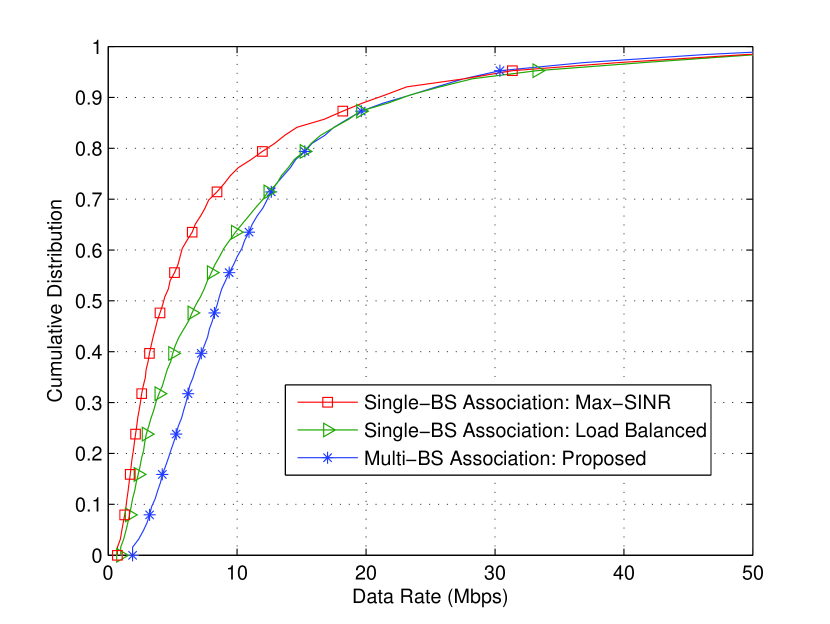
Figure 1: Rate CDFs of single-BS vs. multiple-BS association.

We simulate a 7-cell HetNet deployed on a regular hexagon wrapped around topology, with 1 macro-BS and 3 pico-BSs per cell. A total of 63 users are uniformly distributed throughout the network. The downlink distance-dependent pathloss is modeled as $128.1+37.6\log_{10}d$, where $d$ represents the BS-to-user distance in km; the shadowing effect is modeled as a zero-mean Gaussian random variable with 8dB standard deviation. The total bandwidth is 10MHz, divided into 16 equal bands. The background noise PSD is -169dBm/Hz; the max transmit PSD of macro-BS is -27dBm/Hz; the max transmit PSD of pico-BS is -47dBm/Hz. The on-power of macro-BS is 1450W; the on-power of pico-BS is 21.32W. Two single-BS association schemes are included as benchmarks: (i) Max-SINR scheme, which assigns each user to the BS with the highest SINR then performs power control under fixed association; (ii) Load balanced scheme [7], which uses a proportional fairness objective to associate users to BSs followed by power control under fixed association. The allocation variable $\mathbf{X}$ in these two benchmark schemes is also iteratively optimized with $\mathbf{P}$ using Steps 2 and 3 of Algorithm 2.

Fig. 1 compares the cumulative distribution function (CDF) of user rates for multiple-BS vs. single-BS association schemes without power consumption penalty (i.e., when $\lambda=0$). It is observed that the proposed multiple-band multiple-BS association approach significantly outperforms the single-BS association baselines, particularly in the low-rate regime, e.g., the proposed algorithm doubles the 10th percentile rate as compared to single-BS association. We remark that all the user-BS channels are assumed to be flat-fading across the 16 bands in the simulation, so the reported performance gain is entirely due to multiple-BS association but not frequency diversity.

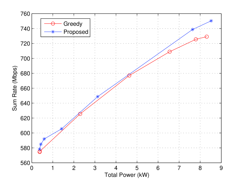
Figure 2: Greedy vs. proposed iteratively reweighting for BS turning-off.

We now evaluate the effectiveness of the proposed algorithms for power optimization and in turning off BSs for power saving. The different points in Fig. 2 are obtained by solving (4) with different $\lambda$ values. It is observed that the proposed algorithm slightly outperforms the greedy method. It should be emphasized that the greedy algorithm is highly sensitive to the initial starting point and the testing sequence of BSs (as in Step 3 of Algorithm 3), which are carefully tuned in this simulation. In particular, we choose to sequentially pick the on-BSs first across the macro BSs, then across the pico BSs, and terminate the algorithm until all on-BSs are picked twice. This testing sequence is believed to be near-optimal in this particular setting because the network model has only two tiers of BSs and their on-power levels differ significantly. In a more complex network, however, it would be more difficult to find a (near-)optimal BS testing sequence. Another drawback of the greedy heuristic is its high complexity, as it involves testing of candidate BSs one at a time, while our proposed algorithm is capable of turning off multiple BSs at the same time through coordinating the proximal updates across the on-BSs. In fact, the proximal update in our simulation has a fast convergence, typically within 30 iterations. As the greedy algorithm requires a centralized evaluation of the total network utility after every BS-deactivation attempt, its computational complexity would be prohibitively high when a large number of BSs are deployed in the network.

V Conclusion

This letter illustrates the benefit of providing the BSs with the flexibility of varying transmit PSDs and possibly being turned off, and providing the users with the flexibility of associating with multiple BSs across multiple frequency bands in a downlink HetNet. We show that the network utility maximization problem with a power consumption penalty can be solved efficiently using a combination of reweighted sparse optimization, block coordinate ascent, and proximal gradient method. By jointly optimizing the PSD levels across the bands, the multiple-BS association, and the user frequency allocation, the proposed algorithm enables effective balancing between network throughput and power consumption.

Appendix A Lagrangian Dual of Problem (9)

Let $\mathbf{y}^{n}\in\mathbb{R}^{K}$ and $\mathbf{z}^{n}\in\mathbb{R}^{L}$ be the Lagrange multipliers associated with the linear inequality constraints (4e) and (4e), respectively. The Lagrangian function of problem (9) can be written as

$${\mathcal{L}}\left(\mathbf{X}^{n};\mathbf{y}^{n},\mathbf{z}^{n}\right)=\frac{1}{2}\left\|\mathbf{X}^{n}-\tilde{\mathbf{X}}^{n}(s)\right\|^{2}_{\text{F}}-\left(\mathbf{X}^{n}\mathbf{e}_{L}-\mathbf{e}_{K}\right)^{T}\mathbf{y}^{n}\\ -\left((\mathbf{X}^{n})^{T}\mathbf{e}_{K}-\mathbf{e}_{L}\right)^{T}\mathbf{z}^{n}.$$ (18)

After some manipulations, we can rewrite ${\mathcal{L}}\left(\mathbf{X}^{n};\mathbf{y}^{n},\mathbf{z}^{n}\right)$ as

$${\mathcal{L}}\left(\mathbf{X}^{n};\mathbf{y}^{n},\mathbf{z}^{n}\right)=\frac{1}{2}\left\|\mathbf{X}^{n}\right\|^{2}_{\text{F}}-\text{Tr}\left(\mathbf{X}^{n}(\tilde{\mathbf{X}}^{n}(s))^{T}\right)-\mathbf{e}^{T}_{L}(\mathbf{X}^{n})^{T}\mathbf{y}^{n}\\ -\mathbf{e}^{T}_{K}\mathbf{X}^{n}\mathbf{z}^{n}+\mathbf{e}_{K}^{T}\mathbf{y}^{n}+\mathbf{e}_{L}^{T}\mathbf{z}^{n}+\text{const}(\tilde{\mathbf{X}}^{n}(s)),$$ (19)

where $\text{Tr}(\cdot)$ is the trace operator and $\text{const}(\tilde{\mathbf{X}}^{n}(s))$ denotes a constant term depending only on $\tilde{\mathbf{X}}^{n}(s)$. The analytic solution of the Lagrangian problem with fixed dual variables, i.e., $\displaystyle\min_{\mathbf{X}^{n}\geq\bm{0}}{\mathcal{L}}\left(\mathbf{X}^{n};\mathbf{y}^{n},\mathbf{z}^{n}\right),$ is

$$(\mathbf{X}^{n})^{*}=\max\left\{\tilde{\mathbf{X}}^{n}(s)+\mathbf{y}^{n}\mathbf{e}^{T}_{L}+\mathbf{e}_{K}(\mathbf{z}^{n})^{T},\bm{0}\right\}.$$ (20)

Using the fact

$$\frac{1}{2}\left\|\max\left\{\mathbf{C},\bm{0}\right\}\right\|^{2}_{\text{F}}-\text{Tr}\left(\max\left\{\mathbf{C},\bm{0}\right\}\mathbf{C}^{T}\right)=-\frac{1}{2}\left\|\max\left\{\mathbf{C},\bm{0}\right\}\right\|^{2}_{\text{F}}$$

and substituting $\left(\mathbf{X}^{n}\right)^{*}$ in (20) into ${\mathcal{L}}(\mathbf{X}^{n};\mathbf{y}^{n},\mathbf{z}^{n})$ in (19), we obtain

$$\min_{\mathbf{X}^{n}\geq\bm{0}}{\mathcal{L}}\left(\mathbf{X}^{n};\mathbf{y}^{n},\mathbf{z}^{n}\right)\\ =-\frac{1}{2}\left\|\max\left\{\tilde{\mathbf{X}}^{n}(s)+\mathbf{y}^{n}\mathbf{e}^{T}_{L}+\mathbf{e}_{K}(\mathbf{z}^{n})^{T},\bm{0}\right\}\right\|^{2}_{\text{F}}\\ -\mathbf{e}_{K}^{T}\mathbf{y}^{n}-\mathbf{e}_{L}^{T}\mathbf{z}^{n}+\text{const}(\tilde{\mathbf{X}}^{n}).$$ (21)

Therefore, the following Lagrangian dual of problem (9)

$$\underset{\mathbf{y}^{n},\,\mathbf{z}^{n}}{\text{max}} \min_{\mathbf{X}^{n}\geq\bm{0}}{\mathcal{L}}(\mathbf{X}^{n};\mathbf{y}^{n},\mathbf{z}^{n})$$ (22a)

s.t. $$\mathbf{y}^{n}\leq\bm{0}$$ (22c)

$$\mathbf{z}^{n}\leq\bm{0}$$

can be equivalently rewritten as problem (10).

Appendix B Closed-Form Solution of Problem (13)

The optimality condition [24] of problem (13) is

$$\mathbf{p}_{\ell}-\tilde{\mathbf{p}}_{\ell}(s+1)+t_{\ell}(s+1)\bm{\xi}=\bm{0},$$ (23)

where $\bm{\xi}\in\partial\|\mathbf{p}_{\ell}\|_{2}$ and $\partial\|\mathbf{p}_{\ell}\|_{2}$ is the subdifferential of the nonsmooth function $\|\mathbf{p}_{\ell}\|_{2}.$ It is simple to compute

$$\partial\|\mathbf{p}_{\ell}\|_{2}=\left\{\begin{array}[]{cl}\mathbf{p}_{\ell}/\|\mathbf{p}_{\ell}\|_{2},&\text{if~{}}\mathbf{p}_{\ell}\neq\bm{0};\\[5.0pt] \displaystyle\left\{\bm{\xi}\,|\,\|\bm{\xi}\|_{2}\leq 1\right\},&\text{if~{}}\mathbf{p}_{\ell}=\bm{0}.\end{array}\right.$$

Let $\mathbf{p}^{*}_{\ell}$ denote the optimal solution of problem (13). Now, we consider the following two cases separately.

• Case I: $t_{\ell}(s+1)\geq\|\tilde{\mathbf{p}}_{\ell}(s+1)\|_{2}.$ We show that $\mathbf{p}^{*}_{\ell}=\bm{0}$ is the optimal solution of problem (13) in this case. Let

  $$\bm{\xi}^{*}=\frac{\tilde{\mathbf{p}}_{\ell}(s+1)}{t_{\ell}(s+1)}.$$

  Then, $\|\bm{\xi}^{*}\|_{2}\leq 1$ and thus $\bm{\xi}^{*}\in\partial\|\mathbf{p}^{*}_{\ell}\|_{2}.$ Moreover, it is simple to check that $\mathbf{p}^{*}_{\ell}$ and $\bm{\xi}^{*}$ satisfy (23). This shows that $\mathbf{p}^{*}_{\ell}=\bm{0}$ is the optimal solution of problem (13) when $t_{\ell}(s+1)\geq\|\tilde{\mathbf{p}}_{\ell}(s+1)\|_{2}.$

• Case II: $t_{\ell}(s+1)<\|\tilde{\mathbf{p}}_{\ell}(s+1)\|_{2}.$ First, it is simple to argue (by contradiction) that $\bm{0}$ is not the optimal solution of problem (13) in this case. Therefore, the optimality condition of problem (13) can be equivalently rewritten as follows:

  $$\left(\frac{t_{\ell}(s+1)}{\|\mathbf{p}_{\ell}\|_{2}}+1\right)\mathbf{p}_{\ell}=\tilde{\mathbf{p}}_{\ell}(s+1),$$ (24)

  which implies that $\mathbf{p}^{*}_{\ell}$ and $\tilde{\mathbf{p}}_{\ell}(s+1)$ are of the same direction, i.e.,

  $$\mathbf{p}^{*}_{\ell}=a\tilde{\mathbf{p}}_{\ell}(s+1)\text{ for some }a>0.$$ (25)

  With the above form of $\mathbf{p}^{*}_{\ell}$ plugged in, problem (13) reduces to an optimization problem over the scalar variable $a>0$:

  $$\underset{a>0}{\text{min}}\quad\frac{(a-1)^{2}}{2}\left\|\tilde{\mathbf{p}}_{\ell}(s+1)\right\|_{2}+at_{\ell}(s+1).$$ (26)

  The closed-form solution of the above problem is

  $$a^{*}=1-\frac{t_{\ell}(s+1)}{\|\tilde{\mathbf{p}}_{\ell}(s+1)\|_{2}}>0.$$ (27)

  Hence, $\mathbf{p}^{*}_{\ell}=\left(1-\frac{t_{\ell}(s+1)}{\|\tilde{\mathbf{p}}_{\ell}(s+1)\|_{2}}\right)\tilde{\mathbf{p}}_{\ell}(s+1)$ is the optimal solution of problem (13) when $t_{\ell}(s+1)<\|\tilde{\mathbf{p}}_{\ell}(s+1)\|_{2}.$

From the above cases I and II, we can conclude that (15) is the solution to problem (13).

References

- [1] R. Sun, M. Hong, and Z.-Q. Luo, “Joint downlink base station association and power control for max-min fairness: Computation and complexity,” IEEE J. Sel. Areas Commun., vol. 33, no. 6, pp. 1040–1054, Mar. 2015.
- [2] L. P. Qian, Y. J. Zhang, Y. Wu, and J. Chen, “Joint downlink base station association and power control via benders’ decomposition,” IEEE Trans. Wireless Commun., vol. 12, no. 4, pp. 1651–1665, Mar. 2013.
- [3] V. N. Ha and L. B. Le, “Distributed base station association and power control for heterogeneous cellular networks,” IEEE Trans. Veh. Technol., vol. 63, no. 1, pp. 282–296, July 2013.
- [4] D. Lopez-Perez, X. Chu, and İ. Guvenc, “On the expanded region of picocells in heterogeneous networks,” IEEE J. Sel. Topics Signal Process., vol. 6, no. 3, pp. 281–294, June 2012.
- [5] R. Madan, J. Borran, A. Sampath, N. Bhushan, A. Khandekar, and T. Ji, “Cell association and interference coordination in heterogeneous LTE-A cellular networks,” IEEE J. Sel. Areas Commun., vol. 28, no. 9, pp. 1479–1489, Dec. 2010.
- [6] Q. Ye, B. Rong, Y. Chen, M. Al-Shalash, C. Caramanis, and J. G. Andrews, “User association for load balancing in heterogeneous cellular networks,” IEEE Trans. Wireless Commun., vol. 12, no. 6, pp. 2706–2716, June 2013.
- [7] K. Shen and W. Yu, “Distributed pricing-based user association for downlink heterogeneous cellular networks,” IEEE J. Sel. Areas Commun., vol. 32, no. 6, pp. 1100–1113, June 2014.
- [8] A. Abbasi and M. Ghaderi, “Energy cost reduction in cellular networks through dynamic base station activation,” in IEEE Ann. Int. Conf. Sensing Commun. Netw., June 2014, pp. 363–371.
- [9] S. Ping, A. Aijaz, O. Holland, and A. H. Aghvami, “Green cellular access network operation through dynamic spectrum and traffic load management,” in IEEE 24th Ann. Int. Symp. Personal Indoor Mobile Radio Commun. (PIMRC), Sept. 2013, pp. 2791–2796.
- [10] D. Bethanabhotla, O. Y. Bursalioglu, H. C. Papadopoulos, and G. Caire, “Optimal user-cell association for massive MIMO wireless networks,” IEEE Trans. Wireless Commun., vol. 15, no. 3, pp. 1835–1850, Mar. 2016.
- [11] M. Sanjabi, M. Razaviyayn, and Z.-Q. Luo, “Optimal joint base station assignment and beamforming for heterogeneous networks.” IEEE Trans. Signal Process., vol. 62, no. 8, pp. 1950–1961, Apr. 2014.
- [12] W. C. Liao, M. Hong, Y.-F. Liu, and Z.-Q. Luo, “Base station activation and linear transceiver design for optimal resource management in heterogeneous networks,” IEEE Trans. Signal Process., vol. 62, no. 15, pp. 3939–3952, Aug. 2014.
- [13] M. Yuan and Y. Lin, “Model selection and estimation in regression with grouped variables,” J. R. Stat. Soc. B, vol. 68, no. 1, pp. 49–67, 2006.
- [14] Y. Shi, J. Zhang, and K. Letaief, “Group sparse beamforming for green cloud-RAN,” IEEE Trans. Wireless Commun., vol. 13, no. 5, pp. 2809–2823, May 2014.
- [15] Y.-F. Liu, M. Hong, and E. Song, “Sample approximation-based deflation approaches for chance SINR constrained joint power and admission control,” IEEE Trans. Wireless Commun., vol. 15, no. 7, pp. 4535–4547, Jul. 2016.
- [16] E. J. Candès, M. B. Wakin, and S. P. Boyd, “Enhancing sparsity by reweighted minimization,” J. Fourier Anal. Appl., vol. 14, no. 5, pp. 877–905, 2008.
- [17] M. Razaviyayn, M. Hong, and Z.-Q. Luo, “A unified convergence analysis of block successive minimization methods for nonsmooth optimization,” SIAM J. Optim., vol. 23, no. 2, pp. 1126–1153, 2013.
- [18] Y. Xu and W. Yin, “A block coordinate descent method for multi-convex optimization with applications to nonnegative tensor factorization and completion,” SIAM J. Imaging Sci., vol. 6, no. 3, pp. 1758–1789, 2013.
- [19] P. Tseng and S. Yun, “A coordinate gradient descent method for nonsmooth separable minimization,” Math. Program., vol. 117, no. 1-2, pp. 387–423, 2009.
- [20] P. L. Combettes and J.-C. Pesquet, “Proximal splitting methods in signal processing,” in Fixed-point Algorithms for Inverse Problems in Science and Engineering. Springer New York, 2011, pp. 185–212.
- [21] N. Parikh and S. P. Boyd, “Proximal algorithms,” Found. Trends Optim., vol. 1, no. 3, pp. 127–239, Jan. 2014.
- [22] M. Grant, S. Boyd, and Y. Ye, “CVX: Matlab software for disciplined convex programming [Online],” Available: http://cvxr.com/cvx/, 2008.
- [23] B. Jiang, Y.-F. Liu, and Z. Wen, “Lp-norm regularization algorithms for optimization over permutation matrices,” SIAM J. Optim., vol. 26, no. 4, pp. 2284–2313, 2016.
- [24] R. T. Rockafellar, Convex Analysis. Princeton, NJ, U.S.A.: Priceton University Press, 1970.