Gluon quasidistribution function at one loop

Wei Wang1 111wei.wang@sjtu.edu.cn, Shuai Zhao1 222shuai.zhao@sjtu.edu.cn, Ruilin Zhu2,1 333rlzhu@njnu.edu.cn 1 INPAC, Shanghai Key Laboratory for Particle Physics and Cosmology, School of Physics and Astronomy, Shanghai Jiao Tong University, Shanghai, 200240, China
2 Department of Physics and Institute of Theoretical Physics, Nanjing Normal University, Nanjing, Jiangsu 210023, China
Abstract

We study the unpolarized gluon quasidistribution function in the nucleon at one loop level in the large momentum effective theory. For the quark quasidistribution, power law ultraviolet divergences arise in the cut-off scheme and an important observation is that they all are subjected to Wilson lines. However for the gluon quasidistribution function, we first point out that the linear ultraviolet divergences also exist in the real diagram which is not connected to any Wilson line. We then study the one loop corrections to parton distribution functions in both cut-off scheme and dimensional regularization to deal with the ultraviolet divergences. In addition to the ordinary quark and gluon distributions, we also include the quark to gluon and gluon to quark splitting diagrams. The complete one-loop matching factors between the quasi and light cone parton distribution functions are presented in the cut-off scheme. We derive the $P^{z}$ evolution equation for quasi parton distribution functions, and find that the $P^{z}$ evolution kernels are identical to the DGLAP evolution kernels.

I Introduction

Hadron structures are determined by strong interactions among quarks and gluons. In order to make predictions for high energy process involving hadrons, one must rely the factorization approach. Parton distribution functions (PDFs) are important inputs to evaluate the hadron scattering cross section in the collinear factorization. However, up to date it is still a formidable task to calculate the PDF from first principles because QCD are only well understood in the perturbative regime of short distance phenomena, whereas the long distance interactions require a nonperturbative approach.

The only method that allows to properly explore the nonperturbative interactions is Lattice QCD (LQCD). PDFs are defined as matrix elements of non-local operators located on the light cone. Thus they are time-dependent, and can not be directly calculated on LQCD. With the help of operator product expansion, PDFs can be expressed in terms of a series of moments that are calculable on LQCD in principle. However only the lowest few moments can be computed on LQCD, while the calculation for higher moments is much more involved due to the operator mixing and the noisy signal.

A more realistic and phenomenological approach is often adopted at this stage. One may appeal to some theoretical parametrization of PDFs and fit the free parameters in the parametrization using the experiment data such as DIS and $pp$ collisions data Butterworth:2015oua ; Hou:2016nqm ; Hou:2017khm . Such an approach has reached very high accuracy, for instance one has taken into account the next-to-next-to-leading order in $\alpha_{s}$ for the calculation of partonic cross section. This method keeps the dependence parametrization of PDFs, and also can not cover all the region of the parton longitudinal momentum fraction $x$.

In 2013, a new approach named as the large momentum effective theory (LaMET) was proposed Ji:2013dva ; Ji:2014gla to determine parton distribution functions on the lattice. In this approach, instead of using the correlations of quarks and gluons on the light cone, one makes use of the matrix elements of frame-dependent equal-time correlators in the large momentum limit. The equal-time correlators, defining the quasi parton distribution functions, can be directly investigated on the Lattice QCD. In the $P^{z}\to\infty$ limit, this effective theory allows us to perform a matching between the ordinary PDFs and the quasi ones. Through this way, the light-cone PDFs can be elegantly extracted. Moreover in fact this approach can generally allow one to derive the information of the light cone parton physics from first principles of QCD.

This approach has been developed rapidly, and a number of progresses have been made recently Xiong:2013bka ; Ma:2014jla ; Ma:2014jga ; Ji:2014lra ; Ji:2015qla ; Xiong:2015nua ; Monahan:2015lha ; Jia:2015pxx ; Li:2016amo ; Li:2017udt ; Nam:2017gzm ; Radyushkin:2016hsy ; Radyushkin:2017gjd ; Zhang:2017bzy ; Radyushkin:2017ffo ; Carlson:2017gpk ; Briceno:2017cpo ; Xiong:2017jtn ; Radyushkin:2017cyf ; Constantinou:2017sej ; Rossi:2017muf ; Orginos:2017kos ; Ji:2017rah ; Broniowski:2017wbr . A key issue in this approach concerns the renormalizability of the quasi PDF Ji:2015jwa ; Chen:2016fxx ; Monahan:2016bvm ; Alexandrou:2017huk ; Chen:2017mzz ; Ji:2017oey ; Ishikawa:2017faj ; Green:2017xeu . Using the heavy quark and Wilson line correspondence, an all order formal proof has been presented in Ref. Ji:2017oey . More explicitly, the one loop matching between nonsinglet quark distributions and quasidistributions has been studied in Refs. Xiong:2013bka ; Ma:2014jga , in which the linear power law ultraviolet (UV) divergences have been found in the cut-off scheme. To absorb the linear divergences, an approach using the nondipolar Wilson line has been proposed in Ref. Li:2016amo ; Li:2017udt ; the other one is Wilson line renormalization by including a “mass” counterterm Chen:2016fxx ; Ishikawa:2016znu ; Ji:2017oey ; Ishikawa:2017faj . On the other side, the direct evaluation of the parton distribution functions have also been performed on the lattice in Refs. Lin:2014zya ; Alexandrou:2015rja ; Chen:2016utp ; Bacchetta:2016zjm ; Alexandrou:2017huk ; Chen:2017mzz ; Bali:2017ude ; Yoon:2017qzo , and the accuracy is incredibly increasing.

It has been recognized for a long time that the gluon distribution functions are one of the key input parameters for the physics at hadron colliders. In the production of Higgs boson and heavy quarkonium, contributions from gluon PDFs are dominant over the quark ones Butterworth:2015oua ; Hou:2016nqm ; Hou:2017khm . For these reasons, it is mandatory to explore the quasi PDF for the gluon in the LaMET, which is still not available yet in the literature. The purpose of this paper is to fill this gap. To do so, we will calculate the perturbative function of gluon quasidistribution at one loop level. Both the cut-off and dimensional regularization scheme are employed in our calculation. We will discuss the difficulties in the application of UV cut-off scheme, and all of the matching functions will be presented in dimensional regularization (DR). The splitting functions are also studied. Based on the matching functions, we derive the $P^{z}$ evolution equation for the parton quasidistributions.

The rest of this paper is organized as follows. In Sec. II, we discuss the one loop results for gluon quasidistribution and light cone distribution in the cut-off scheme. In Sec. III, we give the one loop matching results for parton quasidistributions and light cone distributions at the dimensional regularization scheme (DR). The $P^{z}$ evolution equation of parton quasidistributions is also presented. We summarize in the last section. In the appendix, some calculation details in the cut-off scheme and dimensional regularization are relegated to Sec. A and Sec. B, respectively. In both schemes, we have used the finite gluon mass to regulate the infrared divergences, while in the appendix C, we present the results with the offshellness as an infrared regulator.

II Gluon quasidistribution function in LaMET

II.1 Parton distribution functions

PDFs are important inputs to evaluate the hadron scattering cross section in high energy physics. In the case of unpolarized quark distribution in a hadron, the light cone distribution is defined as

$\displaystyle f_{q/H}(x,\mu^{2})$ $\displaystyle=$ $\displaystyle\int\frac{d\xi^{-}}{4\pi}e^{-i\xi^{-}xP^{+}}\langle P|\overline{\psi}(\xi^{-})\gamma^{+}{\cal P}\exp\left(-ig\int^{\xi^{-}}_{0}d\eta A^{+}(\eta)\right)\psi(0)|P\rangle,$ (1)

where $H$ denotes the hadron, and $|P\rangle$ is the hadron state with momentum $P$, $x=k^{+}/P^{+}$ is the longitudinal momentum fraction.

When discussing light-cone distributions we adopt light-cone coordinate, while for quasi PDFs, the ordinary Minkowski coordinates are used. In the light-cone coordinate system, a vector $a$ is expressed as $a=(a^{+},a^{-},\vec{a}_{\perp})=((a^{0}+a^{3})/\sqrt{2},(a^{0}-a^{3})/\sqrt{2},a^{1},a^{2})$. We also have $k\cdot p=k_{\mu}p^{\mu}=g_{\mu\nu}k^{\mu}p^{\nu}=p^{+}k^{-}+p^{-}k^{+}-\vec{p}_{\perp}\cdot\vec{k}_{\perp}$. We introduce two unit light-cone vectors $n_{+}^{\mu}=(0,1,0,0)$, $n_{-}^{\mu}=(1,0,0,0)$ in the light-cone coordinate system, and the transverse metric $g^{\mu\nu}_{\perp}$. In light-cone coordinate system, $g^{\mu\nu}_{\perp}=g^{\mu\nu}-n_{+}^{\mu}n_{-}^{\nu}-n_{-}^{\mu}n_{+}^{\nu}$, and in ordinary Minkowski coordinates it can be written as $g^{\mu\nu}_{\perp}=g^{\mu\nu}+n_{z}^{\mu}n_{z}^{\nu}-n_{0}^{\mu}n_{0}^{\nu}$, where $n_{z}=(0,0,0,-1)$ and $n_{0}=(1,0,0,0)$. The nucleon momentum in the light-cone coordinates is written as $P^{\mu}=(P^{+},M^{2}/(2P^{+}),0,0)$. The above operator in Eq. (1) is non-local and time-dependent.

In the case of unpolarized gluon distribution in the nucleon, the corresponding light cone distribution is defined as Collins:1981uw

$\displaystyle xf_{g/H}(x,\mu^{2})$ $\displaystyle=$ $\displaystyle\int\frac{d\xi^{-}}{2\pi P^{+}}e^{-i\xi^{-}xP^{+}}\langle P|G^{+}_{~{}\mu}(\xi^{-}){\cal P}\exp\left(-ig\int^{\xi^{-}}_{0}d\eta A^{+}(\eta)\right)G^{\mu+}(0)|P\rangle\ .$ (2)

The covariant derivation is defined as $D_{\mu}=\partial_{\mu}+igA_{\mu}$. Then $G_{\mu\nu}=T^{a}G^{a}_{\mu\nu}=-\frac{i}{g}[D_{\mu},D_{\nu}]=T^{a}(\partial_{\mu}A^{a}_{\nu}-\partial_{\nu}A^{a}_{\mu}-gf^{abc}A^{b}_{\mu}A^{c}_{\nu})$.

In LaMET, the quasidistributions are introduced, which can be calculated directly on the lattice. The unpolarized quark quasidistribution is defined as Ji:2013dva

$\displaystyle\tilde{f}_{q/H}(x,\mu^{2},P^{z})$ $\displaystyle=$ $\displaystyle\int\frac{dz}{4\pi}e^{izxP^{z}}\langle P|\overline{\psi}(z)\gamma^{z}{\cal P}\exp\left(-ig\int^{z}_{0}dz^{\prime}_{z}A^{z}(z^{\prime})\right)\psi(0)|P\rangle\ ,$ (3)

where $x=k^{z}/P^{z}$ with the nucleon momentum $P^{z}$. All the fields are at $\xi^{0}=t=0$ and lie along the $\xi^{3}=z$ direction. Correspondingly, the $\gamma^{+}$ is replaced by $\gamma^{z}$ in the expression. The above quantity is non-local and time-independent, which can be simulated on the lattice for any $P^{z}\ll 1/a$, where $a$ is the lattice spacing.

According to the similar extension, the unpolarized gluon quasidistribution can be defined as Ji:2013dva ; Ma:2014jga

$\displaystyle x\tilde{f}_{g/H}(x,\mu^{2},P^{z})$ $\displaystyle=$ $\displaystyle\int\frac{dz}{2\pi P^{z}}e^{izxP^{z}}\langle P|G^{z}_{~{}\mu}(z){\cal P}\exp\left(-ig\int^{z}_{0}d\eta A^{z}(\eta)\right)G^{\mu z}(0)|P\rangle,$ (4)

where $\mu$ sums over the transverse components. The parton gauge link (Wilson line) is defined along the $z$ direction

$\displaystyle W(z_{2},z_{1})=\mathcal{P}\exp\left(-ig\int^{z_{2}}_{z_{1}}dz^{\prime}A^{z}(z^{\prime})\right).$ (5)

For gluon quasidistribution, the gauge link is in adjoint representation. Through the definitions of PDFs, one can obtain

$\displaystyle f_{q/H}(x)=-f_{\bar{q}/H}(-x),~{}~{}\tilde{f}_{q/H}(x)=-\tilde{f}_{\bar{q}/H}(-x),$ (6)

and

$\displaystyle f_{g/H}(x)=-f_{g/H}(-x),~{}~{}\tilde{f}_{g/H}(x)=-\tilde{f}_{g/H}(-x),$ (7)

by exchanging the two quark or gluon fields in the operator definitions. $\bar{q}$ and $\tilde{\bar{q}}$ are the light-cone and quasi distributions of anti-quark.

In the infinite momentum limit, the nucleon can be viewed as a beam of free partons. Employing the language of quantum field theory, the hard parts of parton quasidistributions and standard distributions can be calculated order by order. The nonperturbative parts of quasidistributions can be calculated on the lattice. Thus we can evaluate the light cone distributions through the matching condition between the quasidistributions and standard distributions. In LaMET, the standard distribution and quasidistribution are connected by the factorization formula

$\displaystyle\tilde{f}_{i/H}(x,P^{z})=\int^{1}_{0}\frac{dy}{y}Z_{ij}\left(\frac{x}{y},\frac{\mu}{P^{z}}\right)f_{j/H}(y,\mu).$ (8)

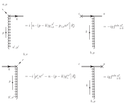
II.2 Feynman rules for gluon quasidistribution function

In the following, we will calculate the gluon quasidistributions in Feynman gauge. The gauge link $W(z,0)$ can be divided into two parts

$\displaystyle W(z,0)=W^{{\dagger}}(+\infty,z)W(+\infty,0),$ (9)

then a half of the matrix element can be written as

$\displaystyle W_{da}(+\infty,z_{1})F_{\mu,a}^{~{}z}(z_{1})$ $\displaystyle=$ $\displaystyle W_{da}(+\infty,z_{1})(\partial_{\mu}A^{z}_{a}-\partial^{z}A_{a,\mu}-gf_{abc}A_{b,\mu}A^{z}_{c}).$ (10)

With the help of integration by parts, the second and the third term of the right side can be rewritten in a compact form

$\displaystyle-\partial^{z}A_{a,\mu}-gf_{abc}A_{b,\mu}A^{z}_{c}=-\partial^{z}(W_{ad}(+\infty,z_{1})A^{d}_{\mu}(z_{1})),$ (11)

then Eq. (10) becomes

$\displaystyle W_{da}(+\infty,z_{1})F_{\mu,a}^{~{}z}(z_{1})$ $\displaystyle=$ $\displaystyle W_{da}(+\infty,z_{1})\partial_{\mu}A^{z}_{a}-\partial^{z}(W_{da}(+\infty,z_{1})A_{a,\mu}).$ (12)

It is obvious that the coupling between the abelian part of field strength tensor and gauge link, and the non-Abelian part of field strength tensor can be reorganized and described by one single Feynman rule. Expanding Eq.(12) to $\mathcal{O}(g^{1})$ in the momentum space will directly lead to the Feynman rule, which is shown in the left panel of Fig. 1. The coupling between eikonal line and gluon is shown in the right panel of Fig. 1.

Refer to caption
Figure 1: Feynman rules for quasi gluon distribution.

II.3 Cut-off scheme

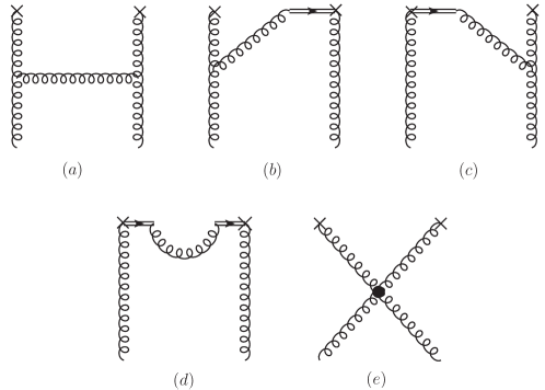
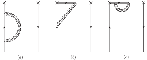
In Feynman gauge, the one-loop diagrams for gluon distribution are depicted in Fig. 2 and Fig. 3. The vertexes from gauge link and non-abelian contributions are incorporated. The gluon mass is introduced to regulate the infrared divergences, and we will use the cut-off scheme to regulate the UV divergences.

Refer to caption
Figure 2: One-loop real corrections to quasi (light-cone) gluon distribution in Feynman gauge. The double line includes both the gauge link and non-abelian contributions.
Refer to caption
Figure 3: One-loop virtual corrections to quasi (light-cone) gluon distribution in Feynman gauge, the conjugate diagrams are not shown. The double line includes both the gauge link and non-abelian contributions.

The one-loop correction can be generally expressed as

$\displaystyle\tilde{f}_{g/g}(x,\Lambda,P^{z})$ $\displaystyle=$ $\displaystyle(1+\delta\tilde{\mathcal{C}}^{(1)}_{gg}(\Lambda,P^{z})+\dots)\delta(x-1)+\tilde{f}_{g/g}^{(1)}(x,\Lambda,P^{z})+\dots,$ (13)

where $\delta\tilde{\mathcal{C}}^{(1)}_{gg}(\Lambda,P^{z})$ accounts for the virtual correction and $\tilde{f}_{g/g}^{(1)}(x,\Lambda,P^{z})$ denotes the real correction.

The contribution from Fig. 2(a) reads

xf~g/g(1)|Fig.2(a)=evaluated-at𝑥superscriptsubscript~𝑓𝑔𝑔1formulae-sequenceFig2𝑎absent\displaystyle x\tilde{f}_{g/g}^{(1)}\bigg{|}_{\mathrm{Fig}.\ref{fig:gluonreal}(a)}= $\displaystyle\int\frac{d^{4}k}{(2\pi)^{4}}(-gf_{a_{1}b_{1}c_{1}}[(P+k)^{\gamma_{1}}g^{\mu_{1}\nu_{1}}+(-2k+P)^{\mu_{1}}g^{\nu_{1}\gamma_{1}}+(k-2P)^{\nu_{1}}g^{\mu_{1}\gamma_{1}}])$
$\displaystyle\times(-gf_{a_{2}b_{2}c_{1}}[(-P-k)^{\gamma_{2}}g^{\mu_{2}\nu_{2}}+(2k-P)^{\mu_{2}}g^{\nu_{2}\gamma_{2}}+(2P-k)^{\nu_{2}}g^{\mu_{2}\gamma_{2}}])$
$\displaystyle\times(i)(k\cdot ng^{\nu^{\prime}_{2}}_{\perp\mu}-n^{\nu^{\prime}_{2}}k_{\perp\mu})(-i)(n^{\nu^{\prime}_{1}}k^{\mu}_{\perp}-k\cdot ng^{\nu^{\prime}_{1}\mu}_{\perp})\delta^{b_{1}}_{b_{2}}\frac{\delta(x-k^{z}/P^{z})}{2(N^{2}_{c}-1)(P^{z})^{2}}$
$\displaystyle\times\frac{-ig_{\nu_{2}\nu^{\prime}_{2}}}{k^{2}-m_{g}^{2}}\frac{-ig_{\nu_{1}\nu^{\prime}_{1}}}{k^{2}-m_{g}^{2}}\frac{-ig_{\gamma_{1}\gamma_{2}}}{(P-k)^{2}-m_{g}^{2}}(-g_{\perp\mu_{1}\mu_{2}}\delta^{a_{1}}_{a_{2}}).$ (14)

A straightforward calculation yields the quasi PDF

f~g/g(1)(x,Pz,Λ)|Fig.2(a)evaluated-atsuperscriptsubscript~𝑓𝑔𝑔1𝑥superscript𝑃𝑧Λformulae-sequenceFig2𝑎\displaystyle\tilde{f}_{g/g}^{(1)}(x,P^{z},\Lambda)\bigg{|}_{\mathrm{Fig}.\ref{fig:gluonreal}(a)} $\displaystyle=\frac{\alpha_{s}C_{A}}{2\pi x}\left\{\begin{array}[]{ll}\left(2x^{3}-3x^{2}+2x-2\right)\ln\frac{x-1}{x}+2x^{2}-\frac{5x}{2}+\frac{8}{3}+\frac{3}{4}\frac{\Lambda}{P^{z}}\ ,&x>1\\ \left(2x^{3}-3x^{2}+2x-2\right)\ln\frac{(x^{2}-x+1)m_{g}^{2}}{4x(1-x)(P^{z})^{2}}+\frac{1}{6}x\left(4x(8x-9)-\frac{9}{(x-1)x+1}+42\right)\\ -\frac{8}{3}+\frac{3}{4}\frac{\Lambda}{P^{z}}\ ,&0<x<1\\ -\left(2x^{3}-3x^{2}+2x-2\right)\ln\frac{x-1}{x}-2x^{2}+\frac{5x}{2}-\frac{8}{3}+\frac{3}{4}\frac{\Lambda}{P^{z}}\ ,&x<0\end{array}\right.$ (19)

and the light-cone PDF

fg/g(1)(x,Λ)|Fig.2(a)evaluated-atsuperscriptsubscript𝑓𝑔𝑔1𝑥Λformulae-sequenceFig2𝑎\displaystyle f_{g/g}^{(1)}(x,\Lambda)\bigg{|}_{\mathrm{Fig}.\ref{fig:gluonreal}(a)} $\displaystyle=\frac{\alpha_{s}C_{A}}{2\pi x}\left\{\begin{array}[]{ll}0\ ,&x>1\ \mbox{or}\ x<0\\ \left(2x^{3}-3x^{2}+2x-2\right)\ln\frac{\left(x^{2}-x+1\right)m_{g}^{2}}{\Lambda^{2}}-\frac{3x}{2(x^{2}-x+1)}+2x^{2}(x-1)+\frac{7}{2}x-2\ ,&0<x<1\end{array}\right.$ (22)

In the above, $\tilde{f}_{g/g}$ and $f_{g/g}$ are quasi and light-cone distributions respectively. One can find that, the infrared divergences, which are regularized as logarithms of $m_{g}^{2}$, are the same in Eqs. (19) and (22). It indicates that the quasi and light-cone distributions have the same infrared structure, and the LaMET factorization holds for the gluon case at one-loop level. The quasi distribution has non-zero values in the region $x>1$ and $x<0$, while the light-cone distribution is zero in these regions. The infrared divergence of quasi distribution only exists in the region $0<x<1$.

A few remarks on the above results are given in order.

  • From the amplitude for Fig. 2(a) given in Eq. (14), one can see that the gluon field strength tensor contributes with a factor $k$, and the three gluon vertex also contributes with a $k$. The $k^{z}$ integration is determined by the $\delta$ function, and thus this amplitude is proportional to

    $\displaystyle\int d^{3}k\frac{k^{4}}{k^{6}}\sim\frac{\Lambda}{P^{z}}.$

    For the light-cone PDF, one finds that this linear divergence is proportional to $n_{+}^{2}$ which vanishes.

  • One can notice that, in light-cone distribution, the UV divergence is logarithmic, while quasi distribution suffers a linear power UV divergence. This will bring an obstacle in the Lattice calculation and need to be properly renormalized. In fact, the linear power divergences have already been discussed in quasi quark distribution, but they only show up in the real diagram where the two pieces of gauge link are connected by a gluon line. Based on this fact, a small mass counter term of gauge link is introduced to deal with the divergence Chen:2016fxx ; Ji:2017oey ; Ishikawa:2016znu . However, in the gluon case, the linear power divergence appears in Eq. (19) and has nothing to do with the Wilson line. It indicates that linear power UV divergence in gluon case must be treated in a different approach. For Figs. 2(b) and (c) where the gluon gauge link participate in, the linear divergence exists as well. Results for these diagrams will be arranged to appendix A.

  • A more severe difficulty in applying the UV cut-off scheme to quasi gluon distribution comes from self-energy diagram Fig. (3a). It is well known that the cut-off scheme for the vacuum polarization will suffer quadratic divergence, even in QED. The source of this divergence is that an UV cut-off will break the gauge symmetry. In the following, we will perform our calculation in DR scheme. However, it would be valuable to find out a cut-off scheme respecting the gauge invariance when calculating in lattice perturbation theory.

  • We have checked that if the index $\mu$ also runs over the time component, i.e. $\mu=0,1,2$, the results for the quasi-PDF are linearly divergent as well.

  • We should note that there are also contributions from the “crossed” diagrams, which can be obtained by exchanging the two gluon lines entering the non-local vertex. They give non-zero contributions to light-cone distribution in the region $-1<x<0$, and for quasi distribution, they contribute to the region $x>0$, $-1<x<0$, and $x<-1$. The “crossed” diagrams and their contributions are not explicitly shown in this work, since their contributions can be easily derived by using Eq. (7).

III One-loop Results for parton quasidistributions and light cone distributions in Dimensional Regularization

In the literature, the matching of quark quasi-PDF has been performed in both cut-off and dimensional regularization schemes. The calculation in $\overline{\mathrm{MS}}$ scheme is meaningful to the discussions on the multiplicative renormalizability of quasi-PDF Ji:2015jwa and the nonperturbative renormalization in RI/MOM scheme Alexandrou:2017huk ; Chen:2017mzz ; Green:2017xeu ; Lin:2017ani ; Stewart:2017tvs . For these reasons we think that it is also valuable to perform perturbative calculation in DR scheme for gluon quasi PDF, just like the case for quark quasi distribution. Besides, it is also convenient to derive the $P^{z}$ evolution equations in DR scheme.

We also note that lattice collaborations had already performed a few calculations on the lattice and some promising results are obtained Lin:2014zya ; Alexandrou:2015rja , without a renormalization of the linear divergence. Therefore, even the problem of linear ultraviolet divergences is unsolved at present, studying the matching of gluon quasidistribution function in $\overline{\mathrm{MS}}$ scheme shall still provide some information to simulate the gluon PDF on the lattice.

In the following we will present our one-loop calculation for quasi and light-cone distributions of quark and gluon. In the calculation, we will work in the Feynman gauge and adopt the dimensional regularization to regularize the UV divergence. The infrared divergence will be regularized by a small gluon mass $m_{g}$.

III.1 Quark in quark

Refer to caption
Figure 4: One-loop real corrections to quark quasi (light-cone) distributions in Feynman gauge.
Refer to caption
Figure 5: One-loop virtual corrections to quark quasi (light-cone) distributions in Feynman gauge, where the conjugate diagrams are not shown.

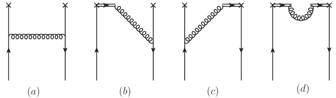
The Feynman diagrams for one-loop corrections to quark in quark distributions are shown in Figs. 4 and 5, where the diagrams in Fig. 4 are the real corrections and the ones in Fig. 5 are the virtual corrections. Similar with gluon distributions, there are also “crossed” diagrams, which can be obtained by exchanging the two quark lines connecting to the non-local vertex. These diagrams can be explained as one-loop corrections to quasi and light-cone distributions of anti-quark. According to Eq. (7), one can immediately recover the anti-quark distributions.

We will calculate the one-loop real corrections to quasi and light-cone quark distributions diagram by diagram. Therein, Fig. 4(a) gives the amplitude

f~q/q(1)(x,μ)|Fig.4(a)evaluated-atsuperscriptsubscript~𝑓𝑞𝑞1𝑥𝜇formulae-sequenceFig4𝑎\displaystyle\tilde{f}_{q/q}^{(1)}(x,\mu)\bigg{|}_{\mathrm{Fig}.\ref{fig:quarkreal}(a)} $\displaystyle=\mu^{2\epsilon}\int\frac{d^{4-2\epsilon}k}{(2\pi)^{4-2\epsilon}}\bar{u}(P)(-igT^{a}\gamma^{\mu})\frac{i}{\not{k}}\gamma^{z}\frac{i}{\not{k}}(-igT^{a}\gamma_{\mu})\frac{-i}{(P-k)^{2}-m_{g}^{2}}u(P)\frac{\delta(x-\frac{k^{z}}{P^{z}})}{4N_{c}P^{z}},$ (23)

which leads to

f~q/q(1)(x,Pz)|Fig.4(a)=αsCF2π{(x1)lnx1x+1,x>1(x1)lnmg24(1x)(Pz)2+x,0<x<1(x1)lnxx11,x<0\displaystyle\tilde{f}_{q/q}^{(1)}(x,P^{z})\bigg{|}_{\mathrm{Fig}.\ref{fig:quarkreal}(a)}=\frac{\alpha_{s}C_{F}}{2\pi}\left\{\begin{aligned} &(x-1)\ln\frac{x-1}{x}+1,~{}~{}&x>1\\ &(x-1)\ln\frac{m_{g}^{2}}{4(1-x)(P^{z})^{2}}+x,~{}~{}&0<x<1\\ &(x-1)\ln\frac{x}{x-1}-1,~{}~{}&x<0\end{aligned}\right. (24)

For the light-cone PDF, we have

fq/q(1)(x,μ)|Fig.4(a)=αsCF2π{0,x>1,x<0(x1)(lnmg2xμ2+2),0<x<1\displaystyle f_{q/q}^{(1)}(x,\mu)\bigg{|}_{\mathrm{Fig}.\ref{fig:quarkreal}(a)}=\frac{\alpha_{s}C_{F}}{2\pi}\left\{\begin{aligned} &0,~{}~{}&x>1,~{}~{}x<0\\ &(x-1)\left(\ln\frac{m_{g}^{2}x}{{\mu}^{2}}+2\right),~{}~{}&0<x<1\end{aligned}\right. (25)

The second and third diagrams have the identical result

f~q/q(1)(x,μ)|Fig.4(b,c)evaluated-atsuperscriptsubscript~𝑓𝑞𝑞1𝑥𝜇formulae-sequenceFig4𝑏𝑐\displaystyle\tilde{f}_{q/q}^{(1)}(x,\mu)\bigg{|}_{\mathrm{Fig}.\ref{fig:quarkreal}(b,c)} $\displaystyle=\mu^{2\epsilon}\int\frac{d^{4-2\epsilon}k}{(2\pi)^{4-2\epsilon}}\bar{u}(P)(igT^{a})\frac{-i}{n\cdot(P-k)}\gamma^{z}\frac{i}{\not{k}}(-igT^{a}\gamma^{z})\frac{-i}{(P-k)^{2}-m_{g}^{2}}u(P)\frac{\delta(x-\frac{k^{z}}{P^{z}})}{4N_{c}P^{z}}.$ (26)

The contributions to quasi PDFs are derived as:

f~q/q(1)(x,Pz)|Fig.4(b)=f~q/q(1)(x,Pz)|Fig.4(c)=αsCF4π{2x1xlnxx111x,x>12x1xln4(1x)(Pz)2mg2+12x1x,0<x<12x1xlnx1x+11x,x<0\displaystyle\tilde{f}_{q/q}^{(1)}(x,P^{z})\bigg{|}_{\mathrm{Fig}.\ref{fig:quarkreal}(b)}=\tilde{f}_{q/q}^{(1)}(x,P^{z})\bigg{|}_{\mathrm{Fig}.\ref{fig:quarkreal}(c)}=\frac{\alpha_{s}C_{F}}{4\pi}\left\{\begin{aligned} &\frac{2x}{1-x}\ln\frac{x}{x-1}-\frac{1}{1-x},~{}~{}~{}~{}&x>1\\ &\frac{2x}{1-x}\ln\frac{4(1-x)(P^{z})^{2}}{m_{g}^{2}}+\frac{1-2x}{1-x},~{}~{}~{}~{}&0<x<1\\ &\frac{2x}{1-x}\ln\frac{x-1}{x}+\frac{1}{1-x},~{}~{}~{}~{}&x<0\end{aligned}\right. (27)

While for the light-cone PDF, we have

fq/q(1)(x,μ2)|Fig.4(b)=fq/q(1)(x,μ2)|Fig.4(c)=αsCF2π{0,x>1,x<0x1xlnμ2mg2x,0<x<1\displaystyle f_{q/q}^{(1)}(x,\mu^{2})\bigg{|}_{\mathrm{Fig}.\ref{fig:quarkreal}(b)}=f_{q/q}^{(1)}(x,\mu^{2})\bigg{|}_{\mathrm{Fig}.\ref{fig:quarkreal}(c)}=\frac{\alpha_{s}C_{F}}{2\pi}\left\{\begin{aligned} &0,~{}~{}~{}~{}&x>1,~{}x<0\\ &\frac{x}{1-x}\ln\frac{\mu^{2}}{m_{g}^{2}x},~{}~{}~{}~{}&0<x<1\end{aligned}\right. (28)

Fig. 4(d) gives

f~q/q(1)|Fig.4(d)evaluated-atsuperscriptsubscript~𝑓𝑞𝑞1formulae-sequenceFig4𝑑\displaystyle\tilde{f}_{q/q}^{(1)}\bigg{|}_{\mathrm{Fig}.\ref{fig:quarkreal}(d)} $\displaystyle=\mu^{2\epsilon}\int\frac{d^{4-2\epsilon}k}{(2\pi)^{4-2\epsilon}}\bar{u}(P)\gamma^{z}(igT^{a})(-igT^{a})n^{2}\frac{-i}{n\cdot(P-k)}\frac{i}{n\cdot(P-k)}\frac{-i}{(P-k)^{2}-m_{g}^{2}}u(P)\frac{\delta(x-\frac{k^{z}}{P^{z}})}{4N_{c}P^{z}},$ (29)

which corresponds to

f~q/q(1)(x)|Fig.4(d)=αsCF2π{11x,x>11x1,0<x<11x1,x<0\displaystyle\tilde{f}_{q/q}^{(1)}(x)\bigg{|}_{\mathrm{Fig}.\ref{fig:quarkreal}(d)}=\frac{\alpha_{s}C_{F}}{2\pi}\left\{\begin{aligned} &\frac{1}{1-x},~{}~{}~{}~{}&x>1\\ &\frac{1}{x-1},~{}~{}~{}~{}&0<x<1\\ &\frac{1}{x-1},~{}~{}~{}~{}&x<0\end{aligned}\right. (30)

The light-cone PDF receives no contribution from this diagram since $n^{2}\equiv n^{2}_{+}=0$:

fq/q(1)(x,μ2)|Fig.4(d)=0.evaluated-atsuperscriptsubscript𝑓𝑞𝑞1𝑥superscript𝜇2formulae-sequenceFig4𝑑0\displaystyle f_{q/q}^{(1)}(x,\mu^{2})\bigg{|}_{\mathrm{Fig}.\ref{fig:quarkreal}(d)}=0. (31)

Next we will calculate the virtual corrections, where their conjugate diagrams contributions are included. The quark self energy diagram will give

δ𝒞~qq(1)|Fig.5(a)=αsCF2πdy{(y1)lny1y+1,y>1(y1)lnmg24(1y)(Pz)2+y,0<y<1(1y)lny1y1,y<0\displaystyle\delta\widetilde{\mathcal{C}}_{qq}^{(1)}\bigg{|}_{\mathrm{Fig}.\ref{fig:quarkvirtual}(a)}=-\frac{\alpha_{s}C_{F}}{2\pi}\int dy\left\{\begin{aligned} &(y-1)\ln\frac{y-1}{y}+1,~{}~{}&y>1\\ &(y-1)\ln\frac{m_{g}^{2}}{4(1-y)(P^{z})^{2}}+y,~{}~{}&0<y<1\\ &(1-y)\ln\frac{y-1}{y}-1,~{}~{}~{}~{}&y<0\end{aligned}\right. (32)

and

δ𝒞qq(1)|Fig.5(a)=αsCF2π01𝑑yy(lnμ2mg2y1).evaluated-at𝛿subscriptsuperscript𝒞1𝑞𝑞formulae-sequenceFig5𝑎subscript𝛼𝑠subscript𝐶𝐹2𝜋subscriptsuperscript10differential-d𝑦𝑦superscript𝜇2superscriptsubscript𝑚𝑔2𝑦1\displaystyle\delta\mathcal{C}^{(1)}_{qq}\bigg{|}_{\mathrm{Fig}.\ref{fig:quarkvirtual}(a)}=-\frac{\alpha_{s}C_{F}}{2\pi}\int^{1}_{0}dy~{}y\left(\ln\frac{\mu^{2}}{m_{g}^{2}y}-1\right). (33)

Fig. 5(b) gives

𝒞~qq(1)|Fig.5(b)evaluated-atsubscriptsuperscript~𝒞1𝑞𝑞formulae-sequenceFig5𝑏\displaystyle\tilde{\mathcal{C}}^{(1)}_{qq}\bigg{|}_{\mathrm{Fig}.\ref{fig:quarkvirtual}(b)} $\displaystyle=\mu^{2\epsilon}\int\frac{d^{4-2\epsilon}k}{(2\pi)^{4-2\epsilon}}\bar{u}(P)(-igT^{a})\frac{-i}{n\cdot(P-k)}\gamma^{z}\frac{i}{\not{k}}(-igT^{a}\gamma^{z})\frac{-i}{(P-k)^{2}-m_{g}^{2}}u(P)\frac{\delta(x-1)}{4N_{c}P^{z}},$ (34)

and thus

δ𝒞~qq(1)|Fig.5(b)=αsCF2πdy{2y1ylnyy111y,y>12y1yln4(1y)(Pz)2mg2+12y1y,0<y<12y1ylny1y+11y,y<0\displaystyle\delta\widetilde{\mathcal{C}}^{(1)}_{qq}\bigg{|}_{\mathrm{Fig}.\ref{fig:quarkvirtual}(b)}=-\frac{\alpha_{s}C_{F}}{2\pi}\int dy\left\{\begin{aligned} &\frac{2y}{1-y}\ln\frac{y}{y-1}-\frac{1}{1-y},~{}~{}&y>1\\ &\frac{2y}{1-y}\ln\frac{4(1-y)(P^{z})^{2}}{m_{g}^{2}}+\frac{1-2y}{1-y},~{}~{}&0<y<1\\ &\frac{2y}{1-y}\ln\frac{y-1}{y}+\frac{1}{1-y},~{}~{}&y<0\end{aligned}\right. (35)

The corrections for light-cone PDF are

δ𝒞qq(1)|Fig.5(b)=αsCF2π01𝑑y2y1ylnμ2mg2y.evaluated-at𝛿subscriptsuperscript𝒞1𝑞𝑞formulae-sequenceFig5𝑏subscript𝛼𝑠subscript𝐶𝐹2𝜋subscriptsuperscript10differential-d𝑦2𝑦1𝑦superscript𝜇2superscriptsubscript𝑚𝑔2𝑦\displaystyle\delta\mathcal{C}^{(1)}_{qq}\bigg{|}_{\mathrm{Fig}.\ref{fig:quarkvirtual}(b)}=-\frac{\alpha_{s}C_{F}}{2\pi}\int^{1}_{0}dy\frac{2y}{1-y}\ln\frac{\mu^{2}}{m_{g}^{2}y}. (36)

Fig. 5(c) gives the amplitude

𝒞~qq(1)|Fig.5(c)evaluated-atsubscriptsuperscript~𝒞1𝑞𝑞formulae-sequenceFig5𝑐\displaystyle\tilde{\mathcal{C}}^{(1)}_{qq}\bigg{|}_{\mathrm{Fig}.\ref{fig:quarkvirtual}(c)} $\displaystyle=\mu^{2\epsilon}\int\frac{d^{4-2\epsilon}k}{(2\pi)^{4-2\epsilon}}\bar{u}(P)\gamma^{z}(-igT^{a})(-igT^{a})n^{2}\frac{-i}{n\cdot(P-k)}\frac{i}{n\cdot(P-k)}\frac{-i}{(P-k)^{2}-m_{g}^{2}}u(P)\frac{\delta(x-1)}{4N_{c}P^{z}}.$ (37)

Corrections to quasi-PDF are then derived as

δ𝒞~qq(1)|Fig.5(c)=αsCF2π{11y,y>11y1,0<y<11y1,y<0\displaystyle\delta\widetilde{\mathcal{C}}^{(1)}_{qq}\bigg{|}_{\mathrm{Fig}.\ref{fig:quarkvirtual}(c)}=-\frac{\alpha_{s}C_{F}}{2\pi}\left\{\begin{aligned} &\frac{1}{1-y},~{}~{}~{}~{}&y>1\\ &\frac{1}{y-1},~{}~{}~{}~{}&0<y<1\\ &\frac{1}{y-1},~{}~{}~{}~{}&y<0\end{aligned}\right. (38)

and for the light-cone, it is again vanishing

δ𝒞qq(1)|Fig.5(c)=0.evaluated-at𝛿subscriptsuperscript𝒞1𝑞𝑞formulae-sequenceFig5𝑐0\displaystyle\delta\mathcal{C}^{(1)}_{qq}\bigg{|}_{\mathrm{Fig}.\ref{fig:quarkvirtual}(c)}=0. (39)

III.2 Gluon in gluon

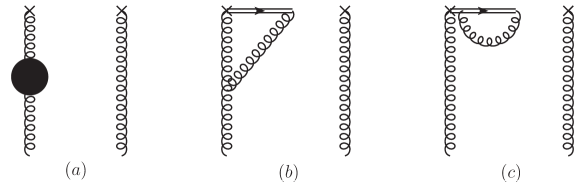
The Feynman diagrams for one-loop corrections to gluon quasi and light-cone distributions have been shown in Fig. 2 and Fig. 3, where the diagrams in Fig. 2 are for real corrections and the diagrams in Fig. 3 are for virtual corrections.

For the real corrections, we have

f~g/g(1)(x,Pz)|Fig.2(a)evaluated-atsuperscriptsubscript~𝑓𝑔𝑔1𝑥superscript𝑃𝑧formulae-sequenceFig2𝑎\displaystyle\tilde{f}_{g/g}^{(1)}(x,P^{z})\bigg{|}_{\mathrm{Fig}.\ref{fig:gluonreal}(a)} $\displaystyle=\frac{\alpha_{s}C_{A}}{2\pi x}\left\{\begin{array}[]{ll}\left(2x^{3}-3x^{2}+2x-2\right)\ln\frac{x-1}{x}+2x^{2}-\frac{5x}{2}+\frac{8}{3}\ ,&x>1\\ \left(2x^{3}-3x^{2}+2x-2\right)\ln\frac{(x^{2}-x+1)m_{g}^{2}}{4x(1-x)(P^{z})^{2}}+\frac{x}{6}\left(4x(8x-9)-\frac{9}{(x-1)x+1}+42\right)-\frac{8}{3}\ ,&0<x<1\\ -\left(2x^{3}-3x^{2}+2x-2\right)\ln\frac{x-1}{x}-2x^{2}+\frac{5x}{2}-\frac{8}{3}\ ,&x<0\end{array}\right.$ (43)

and

fg/g(1)(x,μ)|Fig.2(a)evaluated-atsuperscriptsubscript𝑓𝑔𝑔1𝑥𝜇formulae-sequenceFig2𝑎\displaystyle f_{g/g}^{(1)}(x,\mu)\bigg{|}_{\mathrm{Fig}.\ref{fig:gluonreal}(a)} $\displaystyle=\frac{\alpha_{s}C_{A}}{2\pi x}\left\{\begin{array}[]{ll}0\ ,&x>1\ \mbox{or}\ x<0\\ \left(2x^{3}-3x^{2}+2x-2\right)\ln\frac{\left(x^{2}-x+1\right)m_{g}^{2}}{\mu^{2}}-\frac{3x}{2(x^{2}-x+1)}+2x^{2}(x-1)+\frac{7}{2}x-2\ ,&0<x<1\end{array}\right.$ (46)

Fig. 2(b) yields

xf~g/g(1)|Fig.2(b)=evaluated-at𝑥superscriptsubscript~𝑓𝑔𝑔1formulae-sequenceFig2𝑏absent\displaystyle x\tilde{f}_{g/g}^{(1)}\bigg{|}_{\mathrm{Fig}.\ref{fig:gluonreal}(b)}= $\displaystyle\mu^{2\epsilon}\int\frac{d^{4-2\epsilon}k}{(2\pi)^{4-2\epsilon}}(-gf_{a_{1}b_{1}c_{1}}[(P+k)^{\gamma_{1}}g^{\mu_{1}\nu_{1}}+(-2k+P)^{\mu_{1}}g^{\nu_{1}\gamma_{1}}+(k-2P)^{\nu_{1}}g^{\mu_{1}\gamma_{1}}])$
$\displaystyle\times(i)(k\cdot ng^{~{}\mu_{2}}_{\perp\mu}-n^{\mu_{2}}P_{\perp\mu})(-i)(n^{\nu^{\prime}_{1}}k^{\mu}_{\perp}-k\cdot ng^{\nu^{\prime}_{1}\mu}_{\perp})\frac{\delta(x-k^{z}/P^{z})}{2(N^{2}_{c}-1)(P^{z})^{2}}\frac{-i}{(P-k)\cdot n}(-gf_{a_{2}c_{1}b_{1}}n^{\gamma_{2}})$
$\displaystyle\times\frac{-ig_{\nu_{1}\nu^{\prime}_{1}}}{k^{2}-m_{g}^{2}}\frac{-ig_{\gamma_{1}\gamma_{2}}}{(P-k)^{2}-m_{g}^{2}}(-g_{\perp\mu_{1}\mu_{2}}\delta^{a_{1}}_{a_{2}}),$ (47)

which leads to

f~g/g(1)(x,Pz)|Fig.2(b,c)=αsCA4π{1x1[x(1+x)lnxx12x+1],x>11x1[x(1+x)ln4x(1x)(Pz)2(1x+x2)mg2(2x22x+1)],0<x<11x1[x(1+x)lnx1x+2x1],x<0\displaystyle\tilde{f}_{g/g}^{(1)}(x,P^{z})\bigg{|}_{\mathrm{Fig}.\ref{fig:gluonreal}(b,c)}=-\frac{\alpha_{s}C_{A}}{4\pi}\left\{\begin{aligned} &\frac{1}{x-1}\left[x(1+x)\ln\frac{x}{x-1}-2x+1\right],~{}~{}~{}~{}&x>1\\ &\frac{1}{x-1}\left[x(1+x)\ln\frac{4x(1-x)(P^{z})^{2}}{(1-x+x^{2})m_{g}^{2}}-(2x^{2}-2x+1)\right],~{}~{}~{}~{}&0<x<1\\ &\frac{1}{x-1}\left[x(1+x)\ln\frac{x-1}{x}+2x-1\right],~{}~{}~{}~{}&x<0\end{aligned}\right. (48)

and

fg/g(1)(x,μ)|Fig.2(b)=fg/g(1)(x,μ)|Fig.2(c)=αsCA4π{0,x>1,x<0x(1+x)x1lnμ2mg2(1x+x2),0<x<1\displaystyle f_{g/g}^{(1)}(x,\mu)\bigg{|}_{\mathrm{Fig}.\ref{fig:gluonreal}(b)}=f_{g/g}^{(1)}(x,\mu)\bigg{|}_{\mathrm{Fig}.\ref{fig:gluonreal}(c)}=-\frac{\alpha_{s}C_{A}}{4\pi}\left\{\begin{aligned} &0,~{}~{}~{}~{}&x>1,~{}x<0\\ &{\frac{x(1+x)}{x-1}\ln\frac{\mu^{2}}{m_{g}^{2}(1-x+x^{2})}},~{}~{}~{}~{}&0<x<1\end{aligned}\right. (49)

Fig. 2(d) gives

xf~g/g(1)|Fig.2(d)=evaluated-at𝑥superscriptsubscript~𝑓𝑔𝑔1formulae-sequenceFig2𝑑absent\displaystyle x\tilde{f}_{g/g}^{(1)}\bigg{|}_{\mathrm{Fig}.\ref{fig:gluonreal}(d)}= $\displaystyle\mu^{2\epsilon}\int\frac{d^{4-2\epsilon}k}{(2\pi)^{4-2\epsilon}}\frac{i}{(P-k)\cdot n}gf_{d_{1}c_{1}a_{1}}n^{\gamma_{1}}\frac{-i}{(P-k)\cdot n}(-gf_{a_{2}c_{1}d_{1}}n^{\gamma_{2}})(i)(k\cdot ng^{\mu_{2}}_{\mu}-n^{\mu_{2}}P_{\mu})$
$\displaystyle\times(-i)(n^{\mu_{1}}P^{\mu}_{\perp}-k\cdot ng^{\mu_{1}\mu}_{\perp})\frac{\delta(x-k^{z}/P^{z})}{2(N^{2}_{c}-1)(P^{z})^{2}}\frac{-ig_{\gamma_{1}\gamma_{2}}}{(P-k)^{2}-m_{g}^{2}}(-g_{\perp\mu_{1}\mu_{2}}\delta^{a_{1}}_{a_{2}}),$ (50)

which leads to

f~g/g(1)(x,Pz)|Fig.2(d)=αsCA2π{x1x,x>1xx1,0<x<1xx1,x<0\displaystyle\tilde{f}_{g/g}^{(1)}(x,P^{z})\bigg{|}_{\mathrm{Fig}.\ref{fig:gluonreal}(d)}=\frac{\alpha_{s}C_{A}}{2\pi}\left\{\begin{aligned} &\frac{x}{1-x},~{}~{}~{}~{}&x>1\\ &\frac{x}{x-1},~{}~{}~{}~{}&0<x<1\\ &\frac{x}{x-1},~{}~{}~{}~{}&x<0\end{aligned}\right. (51)

and the correction to light-cone PDF is

fg/g(1)(x,μ)|Fig.2(d)=0.evaluated-atsuperscriptsubscript𝑓𝑔𝑔1𝑥𝜇formulae-sequenceFig2𝑑0\displaystyle f_{g/g}^{(1)}(x,\mu)\bigg{|}_{\mathrm{Fig}.\ref{fig:gluonreal}(d)}=0. (52)

Fig. 2(e) gives

xf~g/g(1)|Fig.2(e)=evaluated-at𝑥superscriptsubscript~𝑓𝑔𝑔1formulae-sequenceFig2𝑒absent\displaystyle x\tilde{f}_{g/g}^{(1)}\bigg{|}_{\mathrm{Fig}.\ref{fig:gluonreal}(e)}= $\displaystyle\mu^{2\epsilon}\int\frac{d^{4-2\epsilon}k}{(2\pi)^{4-2\epsilon}}[f_{c_{1}b_{2}a_{2}}f_{c_{1}b_{1}a_{1}}(g^{\nu_{1}\nu_{2}}g^{\mu_{1}\mu_{2}}-g^{\mu_{2}\nu_{1}}g^{\mu_{1}\nu_{2}})+f_{c_{1}b_{2}a_{1}}f_{c_{1}b_{1}a_{2}}(g^{\nu_{1}\nu_{2}}g^{\mu_{1}\mu_{2}}-g^{\mu_{1}\nu_{1}}g^{\mu_{2}\nu_{2}})]$
$\displaystyle\times(-ig_{s}^{2})(i)(k\cdot ng^{\nu^{\prime}_{2}}_{\perp\mu}-n^{\nu^{\prime}_{2}}k_{\perp\mu})(-i)(n^{\nu^{\prime}_{1}}k^{\mu}_{\perp}-k\cdot ng^{\nu^{\prime}_{1}\mu}_{\perp})$
$\displaystyle\times\delta^{b_{1}}_{b_{2}}\frac{\delta(x-k^{z}/P^{z})}{2(N^{2}_{c}-1)(P^{z})^{2}}\frac{-ig_{\nu_{1}\nu^{\prime}_{1}}}{k^{2}-m_{g}^{2}}\frac{-ig_{\nu_{2}\nu^{\prime}_{2}}}{k^{2}-m_{g}^{2}}(-g_{\perp\mu_{1}\mu_{2}}\delta^{a_{1}}_{a_{2}}).$ (53)

The amplitude gives

f~g/g(1)(x,Pz)|Fig.2(e)=αsCA2π{12,x>112,0<x<112,x<0\displaystyle\tilde{f}_{g/g}^{(1)}(x,P^{z})\bigg{|}_{\mathrm{Fig}.\ref{fig:gluonreal}(e)}=\frac{\alpha_{s}C_{A}}{2\pi}\left\{\begin{aligned} &\frac{1}{2},~{}~{}~{}~{}&x>1\\ &\frac{1}{2},~{}~{}~{}~{}&0<x<1\\ &-\frac{1}{2},~{}~{}~{}~{}&x<0\end{aligned}\right. (54)

and

fg/g(1)(x,μ)|Fig.2(e)=0.evaluated-atsuperscriptsubscript𝑓𝑔𝑔1𝑥𝜇formulae-sequenceFig2𝑒0\displaystyle f_{g/g}^{(1)}(x,\mu)\bigg{|}_{\mathrm{Fig}.\ref{fig:gluonreal}(e)}=0. (55)
Refer to caption
Figure 6: One-loop gluon self energy

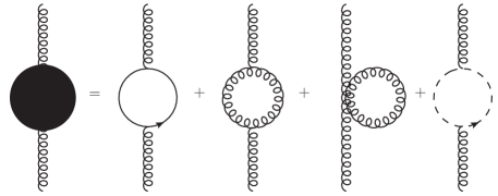
Now we turn to the one-loop virtual corrections. Fig. 3(a) and its conjugate diagram are just the vacuum polarization diagrams of QCD. The black disk denotes the four diagrams which contribute to the gluon self-energy, and these diagrams are shown in Fig. 6. For light-cone PDF, it reads

δ𝒞gg(1)|Fig.3(a)(subtracted)=αs4π[(53CAlnμ2mg243TFnflnμ2mg2)+(5593π)CA203TFnf],evaluated-at𝛿subscriptsuperscript𝒞1𝑔𝑔formulae-sequenceFig3𝑎subtractedsubscript𝛼𝑠4𝜋delimited-[]53subscript𝐶𝐴superscript𝜇2superscriptsubscript𝑚𝑔243subscript𝑇𝐹subscript𝑛𝑓superscript𝜇2superscriptsubscript𝑚𝑔25593𝜋subscript𝐶𝐴203subscript𝑇𝐹subscript𝑛𝑓\displaystyle\delta\mathcal{C}^{(1)}_{gg}\bigg{|}^{(\mathrm{subtracted})}_{\mathrm{Fig}.\ref{fig:gluonvirtual}(a)}=\frac{\alpha_{s}}{4\pi}\left[\left(\frac{5}{3}C_{A}\ln\frac{\mu^{2}}{m_{g}^{2}}-\frac{4}{3}T_{F}n_{f}\ln\frac{\mu^{2}}{-m_{g}^{2}}\right)+\left(\frac{55}{9}-\sqrt{3}\pi\right)C_{A}-\frac{20}{3}T_{F}n_{f}\right], (56)

where $n_{f}$ is the active quark flavor numbers. The UV divergence is subtracted in the $\overline{\mathrm{MS}}$ scheme. For quasi PDF, it contributes

δ𝒞~gg(1)|Fig.3(a)=αs4π[1ϵ(53CA43TFnf)+(53CAlnμ~2mg243TFnflnμ~2mg2)+(5593π)CA203TFnf],evaluated-at𝛿subscriptsuperscript~𝒞1𝑔𝑔formulae-sequenceFig3𝑎subscript𝛼𝑠4𝜋delimited-[]1italic-ϵ53subscript𝐶𝐴43subscript𝑇𝐹subscript𝑛𝑓53subscript𝐶𝐴superscript~𝜇2superscriptsubscript𝑚𝑔243subscript𝑇𝐹subscript𝑛𝑓superscript~𝜇2superscriptsubscript𝑚𝑔25593𝜋subscript𝐶𝐴203subscript𝑇𝐹subscript𝑛𝑓\displaystyle\delta\tilde{\mathcal{C}}^{(1)}_{gg}\bigg{|}_{\mathrm{Fig}.\ref{fig:gluonvirtual}(a)}=\frac{\alpha_{s}}{4\pi}\left[\frac{1}{\epsilon}\left(\frac{5}{3}C_{A}-\frac{4}{3}T_{F}n_{f}\right)+\left(\frac{5}{3}C_{A}\ln\frac{\tilde{\mu}^{2}}{m_{g}^{2}}-\frac{4}{3}T_{F}n_{f}\ln\frac{\tilde{\mu}^{2}}{-m_{g}^{2}}\right)+\left(\frac{55}{9}-\sqrt{3}\pi\right)C_{A}-\frac{20}{3}T_{F}n_{f}\right], (57)

before the UV subtraction. As we have shown in the last section, there is no $\tilde{\mu}$ dependence but $P^{z}$ in the real corrections of quasi PDFs. Therefore, we fix the scale $\tilde{\mu}$ to $P^{z}$ in self-energy correction of the external gluon line and subtract the UV pole. Such a procedure yields

δ𝒞~gg(1)|Fig.3(a)(subtracted)=αs4π[(53CAln(Pz)2mg243TFnfln(Pz)2mg2)+(5593π)CA203TFnf].evaluated-at𝛿subscriptsuperscript~𝒞1𝑔𝑔formulae-sequenceFig3𝑎subtractedsubscript𝛼𝑠4𝜋delimited-[]53subscript𝐶𝐴superscriptsuperscript𝑃𝑧2superscriptsubscript𝑚𝑔243subscript𝑇𝐹subscript𝑛𝑓superscriptsuperscript𝑃𝑧2superscriptsubscript𝑚𝑔25593𝜋subscript𝐶𝐴203subscript𝑇𝐹subscript𝑛𝑓\displaystyle\delta\tilde{\mathcal{C}}^{(1)}_{gg}\bigg{|}^{(\mathrm{subtracted})}_{\mathrm{Fig}.\ref{fig:gluonvirtual}(a)}=\frac{\alpha_{s}}{4\pi}\left[\left(\frac{5}{3}C_{A}\ln\frac{(P^{z})^{2}}{m_{g}^{2}}-\frac{4}{3}T_{F}n_{f}\ln\frac{(P^{z})^{2}}{-m_{g}^{2}}\right)+\left(\frac{55}{9}-\sqrt{3}\pi\right)C_{A}-\frac{20}{3}T_{F}n_{f}\right]. (58)

Fig. (3)(b) leads to

δ𝒞~gg(1)|Fig.3(b)=evaluated-at𝛿subscriptsuperscript~𝒞1𝑔𝑔formulae-sequenceFig3𝑏absent\displaystyle\delta\tilde{\mathcal{C}}^{(1)}_{gg}\bigg{|}_{\mathrm{Fig}.\ref{fig:gluonvirtual}(b)}= $\displaystyle\mu^{2\epsilon}\int\frac{d^{4-2\epsilon}k}{(2\pi)^{4-2\epsilon}}(-gf_{a_{1}b_{1}c_{1}}[(P+k)^{\gamma_{1}}g^{\mu_{1}\nu_{1}}+(-2k+P)^{\mu_{1}}g^{\nu_{1}\gamma_{1}}+(k-2P)^{\nu_{1}}g^{\mu_{1}\gamma_{1}}])$
$\displaystyle\times(i)(n\cdot Pg^{\mu_{2}}_{\perp\mu}-n^{\mu_{2}}P_{\perp\mu})(-i)(n^{\nu^{\prime}_{1}}k^{\mu}_{\perp}-n\cdot Pg^{\nu^{\prime}_{1}\mu}_{\perp})\frac{\delta(x-1)}{2(N^{2}_{c}-1)(P^{z})^{2}}$
$\displaystyle\times\frac{-i}{(P-k)\cdot n}(gf_{a_{2}c_{1}b_{1}}n^{\gamma_{2}})\frac{-ig_{\nu_{1}\nu^{\prime}_{1}}}{k^{2}-m_{g}^{2}}\frac{-ig_{\gamma_{1}\gamma_{2}}}{(P-k)^{2}-m_{g}^{2}}(-g_{\perp\mu_{1}\mu_{2}}\delta^{a_{1}}_{a_{2}}).$ (59)

Including its conjugate diagram, we have

δ𝒞~gg(1)|Fig.3(b)=αsCA2πdy{1+y1ylnyy1+12y1y,y>11+y1yln4y(1y)(Pz)2(1y+y2)mg22y22y+11y,0<y<11+y1ylny1y+2y11y,y<0\displaystyle\delta\tilde{\mathcal{C}}^{(1)}_{gg}\bigg{|}_{\mathrm{Fig}.\ref{fig:gluonvirtual}(b)}=-\frac{\alpha_{s}C_{A}}{2\pi}\int dy\left\{\begin{aligned} &\frac{1+y}{1-y}\ln\frac{y}{y-1}+\frac{1-2y}{1-y},~{}~{}&y>1\\ &\frac{1+y}{1-y}\ln\frac{4y(1-y)(P^{z})^{2}}{(1-y+y^{2})m_{g}^{2}}-\frac{2y^{2}-2y+1}{1-y},~{}~{}&0<y<1\\ &\frac{1+y}{1-y}\ln\frac{y-1}{y}+\frac{2y-1}{1-y},~{}~{}&y<0\end{aligned}\right. (60)

For light-cone PDF we have

δ𝒞gg(1)|Fig.3(b)=αsCA2π01𝑑y1+y1ylnμ2mg2(1y+y2).evaluated-at𝛿subscriptsuperscript𝒞1𝑔𝑔formulae-sequenceFig3𝑏subscript𝛼𝑠subscript𝐶𝐴2𝜋subscriptsuperscript10differential-d𝑦1𝑦1𝑦superscript𝜇2superscriptsubscript𝑚𝑔21𝑦superscript𝑦2\displaystyle\delta\mathcal{C}^{(1)}_{gg}\bigg{|}_{\mathrm{Fig}.\ref{fig:gluonvirtual}(b)}={-\frac{\alpha_{s}C_{A}}{2\pi}\int^{1}_{0}dy\frac{1+y}{1-y}\ln\frac{\mu^{2}}{m_{g}^{2}(1-y+y^{2})}}. (61)

Fig. (3)(c) gives

δ𝒞~gg(1)|Fig.3(c)=evaluated-at𝛿subscriptsuperscript~𝒞1𝑔𝑔formulae-sequenceFig3𝑐absent\displaystyle\delta\tilde{\mathcal{C}}^{(1)}_{gg}\bigg{|}_{\mathrm{Fig}.\ref{fig:gluonvirtual}(c)}= $\displaystyle\mu^{2\epsilon}\int\frac{d^{4-2\epsilon}k}{(2\pi)^{4-2\epsilon}}\frac{i}{(P-k)\cdot n}gf_{d_{1}c_{1}a_{1}}n^{\gamma_{1}}\frac{-i}{(P-k)\cdot n}(gf_{a_{2}c_{2}d_{1}}n^{\gamma_{2}})(i)(n\cdot Pg^{~{}\mu_{2}}_{\perp\mu}-n^{\mu_{2}}P_{\perp\mu})$
$\displaystyle(-i)(n^{\mu_{1}}P^{\mu}_{\perp}-k\cdot ng^{\mu_{1}\mu}_{\perp})\frac{\delta(x-1)}{2(N^{2}_{c}-1)(P^{z})^{2}}\frac{-ig_{\gamma_{1}\gamma_{2}}}{(P-k)^{2}-m_{g}^{2}}(-g_{\perp\mu_{1}\mu_{2}}\delta^{a_{1}}_{a_{2}}).$ (62)

This diagram and its conjugate diagram contribute

δ𝒞~gg(1)|Fig.3(c)=αsCA2πdy{y1y,y>1yy1,0<y<1yy1,y<0\displaystyle\delta\tilde{\mathcal{C}}^{(1)}_{gg}\bigg{|}_{\mathrm{Fig}.\ref{fig:gluonvirtual}(c)}=-\frac{\alpha_{s}C_{A}}{2\pi}\int dy\left\{\begin{aligned} &\frac{y}{1-y},~{}~{}~{}~{}&y>1\\ &\frac{y}{y-1},~{}~{}~{}~{}&0<y<1\\ &\frac{y}{y-1},~{}~{}~{}~{}&y<0\end{aligned}\right. (63)

For light-cone PDF, we have vanishing results:

δ𝒞gg(1)|Fig.3(c)=0.evaluated-at𝛿subscriptsuperscript𝒞1𝑔𝑔formulae-sequenceFig3𝑐0\displaystyle\delta\mathcal{C}^{(1)}_{gg}\bigg{|}_{\mathrm{Fig}.\ref{fig:gluonvirtual}(c)}=0. (64)

According to Eq. (7), the contributions from the “crossed” diagrams can be derived by replacing $x$ with $-x$ and multiplying an additional factor $(-1)$.

III.3 Gluon in quark

Refer to caption
Figure 7: One-loop diagrams for quark splitting to gluon.

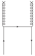
The gluon in quark distribution function is shown in Fig. 7, which gives

$\displaystyle\tilde{f}_{g/q}(x,P^{z})=$ $\displaystyle\mu^{2\epsilon}\int\frac{d^{4-2\epsilon}k}{(2\pi)^{4-2\epsilon}}\bar{u}(P)(-igT^{a}\gamma_{\mu_{2}})\frac{i}{\not{p}-\not{k}}(-igT^{a}\gamma_{\mu_{1}})u(P)$
$\displaystyle\times(i)(k\cdot ng^{\mu_{2}}_{\perp\mu}-n^{\mu_{2}}k_{\perp\mu})(-i)(n^{\mu_{1}}k^{\mu}_{\perp}-k\cdot ng^{\mu_{1}\mu}_{\perp})\frac{-i}{k^{2}-m_{g}^{2}}\frac{-i}{k^{2}-m_{g}^{2}}\frac{\delta(x-\frac{k^{z}}{P^{z}})}{2xN_{c}(P^{z})^{2}},$ (65)

The results for quasi PDF read

$\displaystyle\tilde{f}^{(1)}_{g/q}(x,P^{z})=\frac{\alpha_{s}C_{F}}{2\pi x}\left\{\begin{aligned} &(1+(1-x)^{2})\ln\frac{x}{x-1}-x+\frac{5}{2},~{}~{}~{}~{}&x>1\\ &(1+(1-x)^{2})\ln\frac{4x(P^{z})^{2}}{m_{g}^{2}}-2x^{2}+5x-\frac{5}{2},~{}~{}~{}~{}&0<x<1\\ &(1+(1-x)^{2})\ln\frac{x-1}{x}+x-\frac{5}{2},~{}~{}~{}~{}&x<0\end{aligned}\right.$ (66)

while for light-cone one, we have

$\displaystyle f^{(1)}_{g/q}(x,\mu)=\frac{\alpha_{s}C_{F}}{2\pi x}\left\{\begin{aligned} &0,~{}~{}~{}~{}&x>1,~{}~{}x<0\\ &\left(1+(1-x)^{2}\right)\ln\frac{\mu^{2}}{m_{g}^{2}(1-x)}-2(x^{2}-x+1),~{}~{}&0<x<1\end{aligned}\right.$ (67)

The contributions from the “crossed” diagrams can be derived by using Eq. (7).

III.4 Quark in gluon

Refer to caption
Figure 8: One-loop diagrams for gluon splitting to quark.

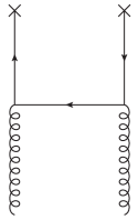
The quark in gluon distribution function is shown in Fig. 8, which contributes to

$\displaystyle\tilde{f}^{(1)}_{q/g}(x,P^{z})=$ $\displaystyle\mu^{2\epsilon}\int\frac{d^{4-2\epsilon}k}{(2\pi)^{4-2\epsilon}}(-1)\mathrm{Tr}\left[\gamma^{z}\frac{i}{\not{k}}(-igT^{a}\gamma^{\mu})\frac{i}{\not{k}-\not{p}}(-igT^{a}\gamma^{\nu})\frac{i}{\not{k}}\right](-g_{\perp\mu\nu})\frac{\delta(x-\frac{k^{z}}{P^{z}})}{4(N_{c}^{2}-1)P^{z}},$ (68)

The result reads

$\displaystyle\widetilde{f}_{q/g}(x,P^{z})=\frac{\alpha_{s}T_{F}}{2\pi}\left\{\begin{aligned} &(x^{2}+(1-x)^{2})\ln\frac{x}{x-1}-2x+1,~{}~{}~{}~{}&x>1\\ &(x^{2}+(1-x)^{2})\ln\frac{4(P^{z})^{2}}{-m_{g}^{2}}-4x^{2}+2x,~{}~{}~{}~{}&0<x<1\\ &(x^{2}+(1-x)^{2})\ln\frac{x-1}{x}+2x-1,~{}~{}~{}~{}&x<0\end{aligned}\right.$ (69)

For light-cone distribution, the result is

$\displaystyle f^{(1)}_{q/g}(x,\mu)=\frac{\alpha_{s}T_{F}}{2\pi}\left\{\begin{aligned} &0,~{}~{}~{}~{}&x>1,~{}~{}x<0\\ &(x^{2}+(1-x)^{2})\ln\frac{\mu^{2}}{-m_{g}^{2}x(1-x)}-1,~{}~{}~{}~{}&0<x<1\end{aligned}\right.$ (70)

The contributions from “crossed” diagrams can be derived by using Eq. (7).

III.5 Matching

In this subsection we perform the matching between the quasi and light-cone PDFs. According to LaMET, if the factorization theorem holds at the leading power of $\mu/P^{z}$, we expect a matching equation as

$\displaystyle\tilde{f}_{i/H}(x,P^{z})=\int^{1}_{0}\frac{dy}{y}Z_{ij}\left(\frac{x}{y},\frac{\mu}{P^{z}}\right)f_{j/H}(y,\mu)\equiv Z_{ij}\left(\xi,\frac{\mu}{P^{z}}\right)\otimes f_{j/H}(y),$ (71)

where $\xi\equiv x/y$, and $i,j$ denotes the involved parton such as quark $q$ and gluon $g$. To perform the perturbative matching, one should first replace the hadron with a parton $k$. Then $\tilde{f}_{i/k}(x,P^{z})$, $f_{j/k}(y,\mu)$ and the matching function $Z_{ij}(\xi,\mu/P^{z})$ can be calculated in perturbation theory. They can be expanded as series of $\alpha_{s}$

$\displaystyle\tilde{f}_{i/k}(x,P^{z})$ $\displaystyle=\sum_{n=0}^{\infty}\tilde{f}^{(n)}_{i/k}(x,P^{z}),$
$\displaystyle f_{j/k}(y,\mu)$ $\displaystyle=\sum_{n=0}^{\infty}f^{(n)}_{j/k}(y,\mu),$
$\displaystyle Z_{ij}\left(\xi,\frac{\mu}{P^{z}}\right)$ $\displaystyle=\sum_{n=0}^{\infty}\left(\frac{\alpha_{s}}{2\pi}\right)^{n}Z^{(n)}_{ij}\left(\xi,\frac{\mu}{P^{z}}\right).$ (72)

where

$\displaystyle f^{(0)}_{j/k}(y)=\delta_{jk}\delta(1-y),~{}~{}~{}~{}\tilde{f}^{(0)}_{i/k}(x)=\delta_{ik}\delta(1-x)$ (73)

are the tree-level distributions. At the order $\mathcal{O}(\alpha^{0}_{s})$, we have $Z^{(0)}_{ij}(\xi,\mu/P^{z})=\delta_{ij}\delta(1-\xi)$.

Then we calculate the matching coefficient $Z^{(1)}_{ij}$. At the order of $\mathcal{O}(\alpha^{1}_{s})$, the matching equation Eq. (71) is reduced to

$\displaystyle\tilde{f}^{(1)}_{i/k}(x,P^{z})$ $\displaystyle=Z^{(0)}_{ij}\left(\xi,\frac{\mu}{P^{z}}\right)\otimes f^{(1)}_{j/k}(y,\mu)+\frac{\alpha_{s}}{2\pi}Z^{(1)}_{ij}\left(\xi,\frac{\mu}{P^{z}}\right)\otimes f^{(0)}_{j/k}(y)$
$\displaystyle=f^{(1)}_{i/k}(x,\mu)+\frac{\alpha_{s}}{2\pi}Z^{(1)}_{ik}\left(x,\frac{\mu}{P^{z}}\right),$ (74)

and then we obtain

$\displaystyle\frac{\alpha_{s}}{2\pi}Z^{(1)}_{ik}\left(x,\frac{\mu}{P^{z}}\right)=\tilde{f}^{(1)}_{i/k}(x,P^{z})-f^{(1)}_{i/k}(x,\mu).$ (75)

Eq. (75) implies that, the one loop correction to the matching function $Z_{ik}(\xi,\mu/P^{z})$, can be derived by taking the difference of the one-loop quasi and LC PDFs. With the one-loop corrections calculated in Sec. III, we have

$\displaystyle Z^{(1)}_{qq}\left(\xi,\frac{\mu}{P^{z}}\right)$ $\displaystyle=C_{F}\left\{\begin{aligned} &-\frac{1+\xi^{2}}{1-\xi}\ln\frac{\xi-1}{\xi}+1,~{}~{}~{}~{}&\xi>1\\ &-\frac{1+\xi^{2}}{1-\xi}\ln\frac{\mu^{2}}{4(P^{z})^{2}\xi(1-\xi)}+\frac{2-5\xi+\xi^{2}}{1-\xi},~{}~{}~{}~{}&0<\xi<1\\ &\frac{1+\xi^{2}}{1-\xi}\ln\frac{\xi-1}{\xi}-1,~{}~{}~{}~{}&\xi<0\end{aligned}\right.$
$\displaystyle+\delta(1-\xi)C_{F}\int d\eta\left\{\begin{aligned} &\frac{1+\eta^{2}}{1-\eta}\ln\frac{\eta-1}{\eta}-1,~{}~{}~{}~{}&\eta>1\\ &\frac{1+\eta^{2}}{1-\eta}\ln\frac{\mu^{2}}{4(P^{z})^{2}\eta(1-\eta)}-\frac{2-5\eta+\eta^{2}}{1-\eta},~{}~{}~{}~{}&0<\eta<1\\ &-\frac{1+\eta^{2}}{1-\eta}\ln\frac{\eta-1}{\eta}+1,~{}~{}~{}~{}&\eta<0\end{aligned}\right.$
$\displaystyle=C_{F}\left\{\begin{aligned} &\left[-\frac{1+\xi^{2}}{1-\xi}\ln\frac{\xi-1}{\xi}+1\right]_{+},~{}~{}~{}~{}&\xi>1\\ &\left[-\frac{1+\xi^{2}}{1-\xi}\ln\frac{\mu^{2}}{4(P^{z})^{2}\xi(1-\xi)}+\frac{2-5\xi+\xi^{2}}{1-\xi}\right]_{+},~{}~{}~{}~{}&0<\xi<1\\ &\left[\frac{1+\xi^{2}}{1-\xi}\ln\frac{\xi-1}{\xi}-1\right]_{+},~{}~{}~{}~{}&\xi<0\end{aligned}\right.$ (76)

where $[\cdots]_{+}$ denotes the “plus” distribution

$\displaystyle\int\left[f(x)\right]_{+}T(x)dx\equiv\int f(x)\left[T(x)-T(1)\right]dx.$ (77)

The above one loop matching factor for quark to quark is equivalent to the result of Ref. Xiong:2013bka . Note that there is a little difference if one directly use the result of Ref. Xiong:2013bka , since therein a cut-off scheme is employed to regularize the UV divergence while a small quark mass is employed to regularize the collinear divergence.

The quark to gluon and gluon to quark ones are given as

$\displaystyle Z^{(1)}_{qg}\left(\xi,\frac{\mu}{P^{z}}\right)$ $\displaystyle=T_{F}\left\{\begin{aligned} &(\xi^{2}+(1-\xi)^{2})\ln\frac{\xi}{\xi-1}-2\xi+1,~{}~{}~{}~{}&\xi>1\\ &-(\xi^{2}+(1-\xi)^{2})\ln\frac{\mu^{2}}{4\xi(1-\xi)(P^{z})^{2}}+1+2\xi-4\xi^{2},~{}~{}~{}~{}&0<\xi<1\\ &-(\xi^{2}+(1-\xi)^{2})\ln\frac{\xi}{\xi-1}+2\xi-1,~{}~{}~{}~{}&\xi<0\\ \end{aligned}\right.$ (78)

and

$\displaystyle Z^{(1)}_{gq}\left(\xi,\frac{\mu}{P^{z}}\right)$ $\displaystyle=C_{F}\left\{\begin{aligned} &\frac{1+(1-\xi)^{2}}{\xi}\ln\frac{\xi}{\xi-1}-1+\frac{5}{2\xi},~{}~{}~{}~{}&\xi>1\\ &-\frac{1+(1-\xi)^{2}}{\xi}\ln\frac{\mu^{2}}{4\xi(1-\xi)(P^{z})^{2}}+3-\frac{1}{2\xi},~{}~{}~{}~{}&0<\xi<1\\ &-\frac{1+(1-\xi)^{2}}{\xi}\ln\frac{\xi}{\xi-1}+1-\frac{5}{2\xi},~{}~{}~{}~{}&\xi<0\\ \end{aligned}\right.$ (79)

The gluon to gluon matching function is given as

$\displaystyle~{}~{}~{}~{}Z^{(1)}_{gg}\left(\xi,\frac{\mu}{P^{z}}\right)$
$\displaystyle=C_{A}\left\{\begin{aligned} &\left(\frac{2\xi^{3}-3\xi^{2}+2\xi-2}{\xi}+\frac{\xi(1+\xi)}{\xi-1}\right)\ln\frac{\xi-1}{\xi}+2\xi-1+\frac{8}{3\xi},~{}~{}~{}~{}&\xi>1\\ &\left(\frac{2\xi^{3}-3\xi^{2}+2\xi-2}{\xi}+\frac{\xi(1+\xi)}{\xi-1}\right)\ln\frac{\mu^{2}}{4\xi(1-\xi)(P^{z})^{2}}\\ &+\frac{10\xi^{2}}{3}-4\xi+4-\frac{2}{3\xi}-\frac{2\xi^{2}-\xi+1}{1-\xi},~{}~{}~{}~{}&0<\xi<1\\ &-\left(\frac{2\xi^{3}-3\xi^{2}+2\xi-2}{\xi}+\frac{\xi(1+\xi)}{\xi-1}\right)\ln\frac{\xi-1}{\xi}-2\xi+1-\frac{8}{3\xi},~{}~{}~{}~{}&\xi<0\\ \end{aligned}\right.$
$\displaystyle~{}~{}~{}~{}-\delta(1-\xi)C_{A}\int d\eta\left\{\begin{aligned} &\frac{1+\eta}{1-\eta}\ln\frac{\eta}{\eta-1}+1,~{}~{}~{}~{}&\eta>1\\ &\frac{1+\eta}{1-\eta}\ln\frac{4\eta(1-\eta)(P^{z})^{2}}{\mu^{2}}-\left(\frac{5}{3}C_{A}-\frac{4}{3}T_{F}n_{f}\right)\ln\frac{(P^{z})^{2}}{\mu^{2}}\\ &-\frac{2\eta^{2}-\eta+1}{1-\eta},~{}~{}~{}~{}&0<\eta<1\\ &-\frac{1+\eta}{1-\eta}\ln\frac{\eta}{\eta-1}-1,~{}~{}~{}~{}&\eta<0\\ \end{aligned}\right.$
$\displaystyle=C_{A}\left\{\begin{aligned} &\frac{2\xi^{3}-3\xi^{2}+2\xi-2}{\xi}\ln\frac{\xi-1}{\xi}+\xi\left[\frac{1+\xi}{\xi-1}\ln\frac{\xi-1}{\xi}+1\right]_{+}+\xi-1+\frac{8}{3\xi},~{}~{}~{}~{}&\xi>1\\ &\frac{2\xi^{3}-3\xi^{2}+2\xi-2}{\xi}\ln\frac{\mu^{2}}{4\xi(1-\xi)(P^{z})^{2}}+\xi\left[\frac{1+\xi}{\xi-1}\ln\frac{\mu^{2}}{4\xi(1-\xi)(P^{z})^{2}}\right]_{+}\\ &+\delta(1-\xi)\left(\frac{5}{3}C_{A}-\frac{4}{3}T_{F}n_{f}\right)\ln\frac{(P^{z})^{2}}{\mu^{2}}-\left[\frac{2\xi^{2}-\xi+1}{1-\xi}\right]_{+}+\frac{10\xi^{2}}{3}-4\xi+4-\frac{2}{3\xi},~{}~{}~{}~{}&0<\xi<1\\ &-\frac{2\xi^{3}-3\xi^{2}+2\xi-2}{\xi}\ln\frac{\xi-1}{\xi}-\xi\left[\frac{1+\xi}{\xi-1}\ln\frac{\xi-1}{\xi}+1\right]_{+}-\xi+1-\frac{8}{3\xi},~{}~{}~{}~{}&\xi<0\\ \end{aligned}\right.$ (80)

Now we consider the contribution from the “crossed” diagrams. As we have discussed in Sec. III, “crossed” diagrams give non-zero contribution to light-cone distributions in $-1<x<0$, and to quasi distributions in $x>0$, $-1<x<0$ and $x<-1$. The contribution from the “uncrossed” and “crossed” diagrams can be related by Eq. (7). For quark, the “crossed” diagrams can be explained as corrections to anti-quark distributions. By replacing $x$ with $-x$ and $y$ with $-y$ in Eq. (71), one can immediately finds that the corrections from “crossed” diagrams share the same matching function $Z(x/y,\mu/P^{z})$. Then, the matching equation Eq. (71) can be extended to

$\displaystyle\tilde{f}_{i/H}(x,P^{z})=\int^{1}_{-1}\frac{dy}{|y|}Z_{ij}\left(\frac{x}{y},\frac{\mu}{P^{z}}\right)f_{j/H}(y,\mu).$ (81)

In this equation, the light-cone distributions have non-zero support in $-1<x<1$. The anti-quark distributions are also included.

III.6 $P^{z}$ evolution equations

From the matching equation Eq. (71) we can derive the evolution equations with $P^{z}$. Notice that the light-cone PDFs is independent of $P^{z}$, one can take the derivative of left and right hand sides of Eq. (71) with $\ln P^{z}$, which yields

$\displaystyle\frac{d\tilde{f}_{i/H}(x,P^{z})}{d\ln P^{z}}$ $\displaystyle=\frac{dZ_{ik}\left(\frac{x}{z},\frac{\mu}{P^{z}}\right)}{d\ln P^{z}}\otimes f_{k/H}(z,\mu)$
$\displaystyle=\frac{dZ_{ik}\left(\frac{x}{z},\frac{\mu}{P^{z}}\right)}{d\ln P^{z}}\otimes\left[Z^{-1}\left(\frac{z}{y},\frac{\mu}{P^{z}}\right)\right]_{kj}\otimes\tilde{f}_{j/H}(y,P^{z})$
$\displaystyle=\frac{d\ln Z_{ij}\left(\frac{x}{y},\frac{\mu}{P^{z}}\right)}{d\ln P^{z}}\otimes\tilde{f}_{j/H}(y,P^{z})$
$\displaystyle=\tilde{P}_{i\leftarrow j}(\xi)\otimes\tilde{f}_{j/H}(y,P^{z}),$ (82)

where $\tilde{P}_{i\leftarrow j}(\xi)\equiv d\ln Z_{ij}(x/y,\mu/P^{z})/d\ln P^{z}$ is the evolution kernel, and $\xi\equiv x/y$. With the matching functions calculated in the last subsection, we obtain the evolution equations at one loop level as follows:

$\displaystyle\frac{d\tilde{f}_{q/H}(x,P^{z})}{d\ln P^{z}}$ $\displaystyle=$ $\displaystyle\frac{\alpha_{s}}{\pi}\int\frac{dy}{y}\left[\tilde{P}_{q\leftarrow q}\left(\frac{x}{y}\right)\tilde{f}_{q/H}\left(y,\frac{\mu}{P^{z}}\right)+\tilde{P}_{q\leftarrow g}\left(\frac{x}{y}\right)\tilde{f}_{g/H}\left(y,\frac{\mu}{P^{z}}\right)\right]\ ,$ (83)
$\displaystyle\frac{d\tilde{f}_{g/H}(x,P^{z})}{d\ln P^{z}}$ $\displaystyle=$ $\displaystyle\frac{\alpha_{s}}{\pi}\int\frac{dy}{y}\left[\tilde{P}_{g\leftarrow q}\left(\frac{x}{y}\right)\sum_{f}\left(\tilde{f}_{q_{f}/H}\left(y,\frac{\mu}{P^{z}}\right)+\tilde{f}_{\bar{q}_{f}/H}\left(y,\frac{\mu}{P^{z}}\right)\right)+\tilde{P}_{g\leftarrow g}\left(\frac{x}{y}\right)\tilde{f}_{g/H}\left(y,\frac{\mu}{P^{z}}\right)\right],$ (84)

where the evolution kernels are

$\displaystyle\tilde{P}_{q\leftarrow q}(\xi)$ $\displaystyle=$ $\displaystyle C_{F}\left\{\begin{array}[]{ll}0\ ,\hskip 71.13188pt\xi>1\ \mbox{or}\ \xi<0\\ \frac{1+\xi^{2}}{(1-\xi)^{+}}+\frac{3}{2}\delta(1-\xi)\ ,\hskip 14.22636pt0<\xi\leq 1\end{array}\right.$ (87)
$\displaystyle\tilde{P}_{q\leftarrow g}(\xi)$ $\displaystyle=$ $\displaystyle T_{F}\left\{\begin{array}[]{ll}0\ ,&\xi>1\ \mbox{or}\ \xi<0\\ \xi^{2}+(1-\xi)^{2}\ ,&0<\xi\leq 1\end{array}\right.$ (90)
$\displaystyle\tilde{P}_{g\leftarrow q}(\xi)$ $\displaystyle=$ $\displaystyle C_{F}\left\{\begin{array}[]{ll}0\ ,&\xi>1\ \mbox{or}\ \xi<0\\ \frac{1+(1-\xi)^{2}}{\xi}\ ,&0<\xi\leq 1\end{array}\right.$ (93)
$\displaystyle\tilde{P}_{g\leftarrow g}(\xi)$ $\displaystyle=$ $\displaystyle\left\{\begin{array}[]{ll}0\ ,\hskip 71.13188pt\xi>1\ \mbox{or}\ \xi<0\\ \frac{2C_{A}(1-\xi+\xi^{2})^{2}}{\xi(1-\xi)^{+}}+\frac{\beta_{0}}{2}\delta(1-\xi)\ ,0<\xi\leq 1\end{array}\right.$ (96)

Here $\beta_{0}=({11C_{A}-2n_{f}})/{3}$. The $P^{z}$ evolution equations of quasi distributions are just the DGLAP equations for the light-cone parton distribution functions Altarelli:1977zs .

IV Conclusions

In this work, we have investigated the unpolarized gluon quasidistribution function in the nucleon at one loop level in the large momentum effective theory. To regularize the ultraviolet divergences, we have adopted the cut-off scheme and the dimensional regularization scheme, while two schemes with finite gluon mass or the offshellness are used to regulate the infrared divergences. In addition to the ordinary quark and gluon distribution functions, we have also studied the quark to gluon and gluon to quark contributions.

When studying the quark quasidistribution in the cut-off scheme, one can find that power law ultraviolet divergences arise in the nonlocal operator and they all are subjected to the Wilson lines. On the contrary in the gluon quasidistribution, we have pointed out in this work that the linear ultraviolet divergences also exist in the real diagram without connecting to the Wilson line. The one loop matching factors between the parton quasi and light cone distribution functions have been derived. Through the simulation on the lattice of the parton quasidistributions, one can finally obtain the nonperturbative information of the parton distributions. At last, we have studied the $P^{z}$ evolution equation for the quasi parton distribution functions, and found that the $P^{z}$ evolution kernels are identical to the DGLAP kernels.

Acknowledgments

We are grateful to Jun Gao, Tomomi Ishikawa, Xiangdong Ji, Yu Jia, Hsiang-Nan Li, Xiaohui Liu, Yanqing Ma, Fan Wang, Feng Yuan, Jianhui Zhang and Yong Zhao for helpful discussions. This work was supported in part by the National Natural Science Foundation of China under Grant No. 11647163, 11575110, 11655002, by Natural Science Foundation of Shanghai under Grant No. 15DZ2272100 and No. 15ZR1423100, by Natural Science Foundation of Jiangsu under Grant No. BK20171471, by the Young Thousand Talents Plan, by Key Laboratory for Particle Physics, Astrophysics and Cosmology, Ministry of Education, and by the Research Start-up Funding of Nanjing Normal University.

Appendix A Cut-off scheme results

In this appendix, we will present the one-loop results for the parton quasi (light cone) distribution functions at the cut-off scheme.

We first take Fig. 2(a) as an example to illustrate the calculation in UV cut-off scheme. By contracting the Lorentz and color indices for Eq. (14), and integrating out the delta function at the non-local vertex, we have the contribution

f~g/g(x,Pz)|Fig.2(a)evaluated-atsubscript~𝑓𝑔𝑔𝑥superscript𝑃𝑧formulae-sequenceFig2𝑎\displaystyle~{}~{}~{}~{}\tilde{f}_{g/g}(x,P^{z})\bigg{|}_{\mathrm{Fig}.\ref{fig:gluonreal}(a)}
$\displaystyle=-\frac{2i\alpha_{s}C_{A}}{xP^{z}}\int\frac{dk^{0}d^{2}k_{\perp}}{(2\pi)^{3}}\frac{1}{\left(-(k^{0})^{2}+k^{2}_{\perp}+m_{g}^{2}+x^{2}(P^{z})^{2}\right)^{2}\left(-(k^{0})^{2}+2k^{0}\sqrt{m_{g}^{2}+(P^{z})^{2}}+k^{2}_{\perp}+(P^{z})^{2}x(x-2)\right)}$
$\displaystyle\times\bigg{[}x^{2}(P^{z})^{2}\left(-(k^{0})^{2}-2k^{0}\sqrt{m_{g}^{2}+(P^{z})^{2}}-m_{g}^{2}+(P^{z})^{2}x(x+2)\right)+2(k^{2}_{\perp})^{2}+k^{2}_{\perp}(P^{z})^{2}(5x^{2}+4)\bigg{]}.$ (97)

The two dominators are given as

$\displaystyle D_{1}$ $\displaystyle\equiv-(k^{0})^{2}+k^{2}_{\perp}+m_{g}^{2}+x^{2}(P^{z})^{2},$
$\displaystyle D_{2}$ $\displaystyle\equiv-(k^{0})^{2}+2k^{0}\sqrt{m_{g}^{2}+(P^{z})^{2}}+k^{2}_{\perp}+(P^{z})^{2}x(x-2).$ (98)

The integral in Eq. (97) can be reduced to five scalar integrals:

$\displaystyle I_{1}$ $\displaystyle=\int\frac{dk^{0}d^{2}k_{\perp}}{(2\pi)^{3}}\frac{(k^{0})^{4}}{D^{2}_{1}D_{2}},$
$\displaystyle I_{2}$ $\displaystyle=\int\frac{dk^{0}d^{2}k_{\perp}}{(2\pi)^{3}}\frac{k^{0}}{D^{2}_{1}D_{2}},$
$\displaystyle I_{3}$ $\displaystyle=\int\frac{dk^{0}d^{2}k_{\perp}}{(2\pi)^{3}}\frac{1}{D^{2}_{1}D_{2}},$
$\displaystyle I_{4}$ $\displaystyle=\int\frac{dk^{0}d^{2}k_{\perp}}{(2\pi)^{3}}\frac{(k^{2}_{\perp})^{2}}{D^{2}_{1}D_{2}},$
$\displaystyle I_{5}$ $\displaystyle=\int\frac{dk^{0}d^{2}k_{\perp}}{(2\pi)^{3}}\frac{k^{2}_{\perp}}{D^{2}_{1}D_{2}}.$ (99)

To calculate these integrals, we perform the Feynman parametrization, and then integrate over $k^{0}$ by using the residue theorem. The remaining integral is the integral over transverse momentum $k_{\perp}$. The possible UV divergence is regularized by introducing a cut off $\Lambda$ on the transverse momentum. The last step is to integrate over the Feynman parameter. Through the above procedure, we arrive at

$\displaystyle I_{1}$ $\displaystyle=-\frac{iP^{z}}{4\pi}\left\{\begin{aligned} &x^{3}\ln\frac{x-1}{x}+x^{2}+\frac{x}{8}+\frac{1}{8(x-1)}+\frac{11}{24}+\frac{3}{8}\frac{\Lambda}{P^{z}},~{}~{}~{}~{}&x>1\\ &x^{3}\ln\frac{(1-x+x^{2})m^{2}_{g}}{4x(1-x)(P^{z})^{2}}-\frac{(x-1)x^{4}(P^{z})^{2}}{2\left(1-x+x^{2}\right)m_{g}^{2}}\\ &+\frac{64x^{8}-216x^{7}+374x^{6}-394x^{5}+252x^{4}-110x^{3}+43x^{2}-24x+8}{24(x-1)(1-x+x^{2})^{2}}+\frac{3}{8}\frac{\Lambda}{P^{z}},&0<x<1\\ &x^{3}\ln\frac{x}{x-1}-x^{2}-\frac{x}{8}-\frac{1}{8(x-1)}-\frac{11}{24}+\frac{3}{8}\frac{\Lambda}{P^{z}},~{}~{}~{}~{}&x<0\end{aligned}\right.$ (100)
$\displaystyle I_{2}$ $\displaystyle=-\frac{i}{16\pi(P^{z})^{2}}\left\{\begin{aligned} &\ln\frac{x-1}{x}+\frac{2x-1}{2x(x-1)},~{}~{}~{}~{}&x>1\\ &\ln\frac{4x(1-x)(P^{z})^{2}}{(1-x+x^{2})m^{2}_{g}}-\frac{2(x-1)x(P^{z})^{2}}{(1-x+x^{2})m^{2}_{g}}+\frac{2x^{6}-6x^{5}+10x^{4}-10x^{3}+2x^{2}+2x-1}{2x(x-1)(1-x+x^{2})^{2}},&0<x<1\\ &-\ln\frac{x-1}{x}-\frac{2x-1}{2x(x-1)},~{}~{}~{}~{}&x<0\end{aligned}\right.$ (101)
$\displaystyle I_{3}$ $\displaystyle=-\frac{i}{32\pi(P^{z})^{3}}\left\{\begin{aligned} &\frac{1}{x^{2}(x-1)},~{}~{}~{}~{}&x>1\\ &-\frac{4(x-1)(P^{z})^{2}}{m^{2}_{g}(1-x+x^{2})}+\frac{2x^{4}-6x^{3}+4x^{2}-2x+1}{(x-1)x^{2}\left(1-x+x^{2}\right)^{2}},&0<x<1\\ &-\frac{1}{x^{2}(x-1)},~{}~{}~{}~{}&x<0\end{aligned}\right.$ (102)
$\displaystyle I_{4}$ $\displaystyle=\frac{iP^{z}}{12\pi}\left\{\begin{aligned} &3x-1-\frac{9}{8}\frac{\Lambda}{P^{z}},~{}~{}~{}~{}&x>1\\ &2x^{3}-3x^{2}+3x-1-\frac{9}{8}\frac{\Lambda}{P^{z}},&0<x<1\\ &-(3x-1)-\frac{9}{8}\frac{\Lambda}{P^{z}},~{}~{}~{}~{}&x<0\end{aligned}\right.$ (103)
$\displaystyle I_{5}$ $\displaystyle=-\frac{i}{8\pi P^{z}}\left\{\begin{aligned} &(x-1)\ln\frac{x-1}{x}+1,~{}~{}~{}~{}&x>1\\ &(x-1)\ln\frac{(1-x+x^{2})m^{2}_{g}}{4x(1-x)(P^{z})^{2}}+2x-1,&0<x<1\\ &-(x-1)\ln\frac{x-1}{x}-1.~{}~{}~{}~{}&x<0\end{aligned}\right.$ (104)

One can find that the integrals $I_{2,3,5}$ are UV finite, but $I_{1}$ and $I_{4}$ are linearly divergent. With these integrals, we finally arrive at Eq. (19), which are linearly divergent as well.

The results for Fig. 2(b) and Fig. 2(c) are given as

f~g/g(1)(x,Pz,Λ)|Fig.2(b,c)=αsCA4π{1x1[x(1+x)lnxx12x+1+ΛPz],x>11x1[x(1+x)ln4x(1x)(Pz)2(1x+x2)mg2(2x22x+1)+ΛPz],0<x<11x1[x(1+x)lnx1x+2x1+ΛPz],x<0\displaystyle\tilde{f}_{g/g}^{(1)}(x,P^{z},\Lambda)\bigg{|}_{\mathrm{Fig}.\ref{fig:gluonreal}(b,c)}=-\frac{\alpha_{s}C_{A}}{4\pi}\left\{\begin{aligned} &\frac{1}{x-1}\left[x(1+x)\ln\frac{x}{x-1}-2x+1+\frac{\Lambda}{P^{z}}\right],~{}~{}~{}~{}&x>1\\ &\frac{1}{x-1}\left[x(1+x)\ln\frac{4x(1-x)(P^{z})^{2}}{(1-x+x^{2})m_{g}^{2}}-(2x^{2}-2x+1)+\frac{\Lambda}{P^{z}}\right],~{}~{}~{}~{}&0<x<1\\ &\frac{1}{x-1}\left[x(1+x)\ln\frac{x-1}{x}+2x-1+\frac{\Lambda}{P^{z}}\right],~{}~{}~{}~{}&x<0\end{aligned}\right. (105)

and

fg/g(1)(x,Λ)|Fig.2(b,c)=αsCA4π{0,x>1,x<0x(1+x)x1lnΛ2mg2(1x+x2),0<x<1\displaystyle f_{g/g}^{(1)}(x,\Lambda)\bigg{|}_{\mathrm{Fig}.\ref{fig:gluonreal}(b,c)}=-\frac{\alpha_{s}C_{A}}{4\pi}\left\{\begin{aligned} &0,~{}~{}~{}~{}&x>1,~{}x<0\\ &{\frac{x(1+x)}{x-1}\ln\frac{\Lambda^{2}}{m_{g}^{2}(1-x+x^{2})}},~{}~{}~{}~{}&0<x<1\end{aligned}\right. (106)

Fig. 2(d) gives

f~g/g(1)(x,Pz,Λ)|Fig.2(d)=αsCA2π{x1x+x(x1)2ΛPz,x>1xx1+x(x1)2ΛPz,0<x<1xx1+x(x1)2ΛPz,x<0\displaystyle\tilde{f}_{g/g}^{(1)}(x,P^{z},\Lambda)\bigg{|}_{\mathrm{Fig}.\ref{fig:gluonreal}(d)}=\frac{\alpha_{s}C_{A}}{2\pi}\left\{\begin{aligned} &\frac{x}{1-x}+\frac{x}{(x-1)^{2}}\frac{\Lambda}{P^{z}},~{}~{}~{}~{}&x>1\\ &\frac{x}{x-1}+\frac{x}{(x-1)^{2}}\frac{\Lambda}{P^{z}},~{}~{}~{}~{}&0<x<1\\ &\frac{x}{x-1}+\frac{x}{(x-1)^{2}}\frac{\Lambda}{P^{z}},~{}~{}~{}~{}&x<0\end{aligned}\right. (107)

and

fg/g(1)(x,Λ)|Fig.2(d)=0.evaluated-atsuperscriptsubscript𝑓𝑔𝑔1𝑥Λformulae-sequenceFig2𝑑0\displaystyle f_{g/g}^{(1)}(x,\Lambda)\bigg{|}_{\mathrm{Fig}.\ref{fig:gluonreal}(d)}=0. (108)

Fig. 2(e) gives

f~g/g(1)(x,Pz,Λ)|Fig.2(e)=αsCA2π{12Λ2xPz,x>112Λ2xPz,0<x<112Λ2xPz,x<0\displaystyle\tilde{f}_{g/g}^{(1)}(x,P^{z},\Lambda)\bigg{|}_{\mathrm{Fig}.\ref{fig:gluonreal}(e)}=\frac{\alpha_{s}C_{A}}{2\pi}\left\{\begin{aligned} &\frac{1}{2}-\frac{\Lambda}{2xP^{z}},~{}~{}~{}~{}&x>1\\ &\frac{1}{2}-\frac{\Lambda}{2xP^{z}},~{}~{}~{}~{}&0<x<1\\ &-\frac{1}{2}-\frac{\Lambda}{2xP^{z}},~{}~{}~{}~{}&x<0\end{aligned}\right. (109)

and

fg/g(1)(x,Λ)|Fig.2(e)=0.evaluated-atsuperscriptsubscript𝑓𝑔𝑔1𝑥Λformulae-sequenceFig2𝑒0\displaystyle f_{g/g}^{(1)}(x,\Lambda)\bigg{|}_{\mathrm{Fig}.\ref{fig:gluonreal}(e)}=0. (110)

For the virtual corrections, Fig. (3)(b) contributes

δ𝒞~gg(1)|Fig.3(b)=αsCA2πdy{1+y1ylnyy1+12y1y+11yΛPz,y>11+y1yln4y(1y)(Pz)2(1y+y2)mg22y22y+11y+11yΛPz,0<y<11+y1ylny1y+2y11y+11yΛPz.y<0\displaystyle\delta\tilde{\mathcal{C}}^{(1)}_{gg}\bigg{|}_{\mathrm{Fig}.\ref{fig:gluonvirtual}(b)}=-\frac{\alpha_{s}C_{A}}{2\pi}\int dy\left\{\begin{aligned} &\frac{1+y}{1-y}\ln\frac{y}{y-1}+\frac{1-2y}{1-y}+\frac{1}{1-y}\frac{\Lambda}{P^{z}},~{}~{}&y>1\\ &\frac{1+y}{1-y}\ln\frac{4y(1-y)(P^{z})^{2}}{(1-y+y^{2})m_{g}^{2}}-\frac{2y^{2}-2y+1}{1-y}+\frac{1}{1-y}\frac{\Lambda}{P^{z}},~{}~{}&0<y<1\\ &\frac{1+y}{1-y}\ln\frac{y-1}{y}+\frac{2y-1}{1-y}+\frac{1}{1-y}\frac{\Lambda}{P^{z}}.~{}~{}&y<0\end{aligned}\right. (111)

to quasi gluon distribution. For light-cone PDF we have

δ𝒞gg(1)|Fig.3(b)=αsCA2π01𝑑y1+y1ylnμ2mg2(1y+y2).evaluated-at𝛿subscriptsuperscript𝒞1𝑔𝑔formulae-sequenceFig3𝑏subscript𝛼𝑠subscript𝐶𝐴2𝜋subscriptsuperscript10differential-d𝑦1𝑦1𝑦superscript𝜇2superscriptsubscript𝑚𝑔21𝑦superscript𝑦2\displaystyle\delta\mathcal{C}^{(1)}_{gg}\bigg{|}_{\mathrm{Fig}.\ref{fig:gluonvirtual}(b)}={-\frac{\alpha_{s}C_{A}}{2\pi}\int^{1}_{0}dy\frac{1+y}{1-y}\ln\frac{\mu^{2}}{m_{g}^{2}(1-y+y^{2})}}. (112)

Fig. 3(c) and its conjugate diagram contribute

δ𝒞~gg(1)|Fig.3(c)=αsCA2πdy{y1y+y(1y)2ΛPz,y>1yy1+y(1y)2ΛPz,0<y<1yy1+y(1y)2ΛPz,y<0\displaystyle\delta\tilde{\mathcal{C}}^{(1)}_{gg}\bigg{|}_{\mathrm{Fig}.\ref{fig:gluonvirtual}(c)}=-\frac{\alpha_{s}C_{A}}{2\pi}\int dy\left\{\begin{aligned} &\frac{y}{1-y}+\frac{y}{(1-y)^{2}}\frac{\Lambda}{P^{z}},~{}~{}~{}~{}&y>1\\ &\frac{y}{y-1}+\frac{y}{(1-y)^{2}}\frac{\Lambda}{P^{z}},~{}~{}~{}~{}&0<y<1\\ &\frac{y}{y-1}+\frac{y}{(1-y)^{2}}\frac{\Lambda}{P^{z}},~{}~{}~{}~{}&y<0\end{aligned}\right. (113)

to quasi gluon distribution. For light-cone PDF, these diagrams vanish since $n_{+}^{2}=0$:

δ𝒞gg(1)|Fig.3(c)=0evaluated-at𝛿subscriptsuperscript𝒞1𝑔𝑔formulae-sequenceFig3𝑐0\displaystyle\delta\mathcal{C}^{(1)}_{gg}\bigg{|}_{\mathrm{Fig}.\ref{fig:gluonvirtual}(c)}=0 (114)

At last we discuss Fig. 3(a), the vacuum polarization diagram of QCD. Due to the Ward identity, the one-loop two-point green function of gluon should be transversely polarized. However, it is well known that a cut-off on the momentum integral breaks the gauge invariance. When the cut-off is imposed on all of the four components of the loop integral, it will lead to a quadratic divergence; when the cut-off is imposed on the transverse momentum integral, which is the case of this work (integrating out “0” component by using residue theorem and keeping $z$ component unintegrated), it will lead to a linear divergence. To evaluate Fig. 3(a) correctly, a cut-off scheme respecting the gauge invariance is needed, instead of a naive cut-off. This implies the linear divergence in the real corrections, as shown in the above, is a consequence of breaking the gauge invariance in the cut-off. For this reason, we can not have reasonable results for Fig. 3(a) at present.

Appendix B Integrals in dimensional regularization

In dimensional regularization scheme, the space-time dimension is shifted from $d=4$ to $d=4-2\epsilon$. However, as we will see below, the real corrections to quasi PDFs is finite in DR scheme.

Again we will briefly demonstrate the calculation method by taking Fig. 2(a) as an example. By contracting the Lorentz indices for Eq. (14), and integrating out the delta function at the non-local vertex, we have

f~g/g(x,Pz)|Fig.2(a)evaluated-atsubscript~𝑓𝑔𝑔𝑥superscript𝑃𝑧formulae-sequenceFig2𝑎\displaystyle~{}~{}~{}~{}\tilde{f}_{g/g}(x,P^{z})\bigg{|}_{\mathrm{Fig}.\ref{fig:gluonreal}(a)}
$\displaystyle=-\frac{2i\alpha_{s}C_{A}\mu^{2\epsilon}}{(d-2)xP^{z}}\int\frac{dk^{0}d^{2-2\epsilon}k_{\perp}}{(2\pi)^{3-2\epsilon}}\frac{1}{\left(-(k^{0})^{2}+k^{2}_{\perp}+m_{g}^{2}+x^{2}(P^{z})^{2}\right)^{2}\left(-(k^{0})^{2}+2k^{0}\sqrt{m_{g}^{2}+(P^{z})^{2}}+k^{2}_{\perp}+(P^{z})^{2}x(x-2)\right)}$
$\displaystyle\times\bigg{[}(d-2)x^{2}(P^{z})^{2}\left(-(k^{0})^{2}-2k^{0}\sqrt{m_{g}^{2}+(P^{z})^{2}}-m_{g}^{2}+(P^{z})^{2}x(x+2)\right)+4(k^{2}_{\perp})^{2}+(d-2)k^{2}_{\perp}(P^{z})^{2}(5x^{2}+4)\bigg{]}.$ (115)

We denote the two dominators as

$\displaystyle D_{1}$ $\displaystyle\equiv-(k^{0})^{2}+k^{2}_{\perp}+m_{g}^{2}+x^{2}(P^{z})^{2},$
$\displaystyle D_{2}$ $\displaystyle\equiv-(k^{0})^{2}+2k^{0}\sqrt{m_{g}^{2}+(P^{z})^{2}}+k^{2}_{\perp}+(P^{z})^{2}x(x-2).$ (116)

The integral can be reduced to five scalar integrals, which are

$\displaystyle I_{1}$ $\displaystyle=\int\frac{dk^{0}d^{2-2\epsilon}k_{\perp}}{(2\pi)^{3-2\epsilon}}\frac{(k^{0})^{4}}{D^{2}_{1}D_{2}},$
$\displaystyle I_{2}$ $\displaystyle=\int\frac{dk^{0}d^{2-2\epsilon}k_{\perp}}{(2\pi)^{3-2\epsilon}}\frac{k^{0}}{D^{2}_{1}D_{2}},$
$\displaystyle I_{3}$ $\displaystyle=\int\frac{dk^{0}d^{2-2\epsilon}k_{\perp}}{(2\pi)^{3-2\epsilon}}\frac{1}{D^{2}_{1}D_{2}},$
$\displaystyle I_{4}$ $\displaystyle=\int\frac{dk^{0}d^{2-2\epsilon}k_{\perp}}{(2\pi)^{3-2\epsilon}}\frac{(k^{2}_{\perp})^{2}}{D^{2}_{1}D_{2}},$
$\displaystyle I_{5}$ $\displaystyle=\int\frac{dk^{0}d^{2-2\epsilon}k_{\perp}}{(2\pi)^{3-2\epsilon}}\frac{k^{2}_{\perp}}{D^{2}_{1}D_{2}}.$ (117)

To calculate these integrals, we perform the Feynman parametrization, then integrate over $k^{0}$ by using the residue theorem. After that, we integrate over the transverse momentum $k_{\perp}$ in $2-2\epsilon$ dimensions. At last, the Feynman parameter $y$ is integrated out.

When integrating over $k_{\perp}$ the following formula is useful:

$\displaystyle\int\frac{d^{D}k_{\perp}}{(2\pi)^{D}}\frac{1}{(k^{2}_{\perp}+\Delta)^{n}}=\frac{1}{(4\pi)^{\frac{D}{2}}}\frac{\Gamma\left(n-\frac{D}{2}\right)}{\Gamma(n)}\frac{1}{\Delta^{n-\frac{D}{2}}}.$ (118)

We should note that this formula is valid only when $\mathrm{Re}\left(n-D/2\right)>0$. For a linearly divergent integral, $n-D/2=-1/2<0$, this formula is not valid. However, under the spirit of analytical continuation, one can assign a finite value to a linearly divergent integral by using Eq. (118). With such analytical continuation, the linearly divergent integrals $I_{1}$ and $I_{4}$ are finite in the dimensional regularization scheme. Therefore, the final result of Fig. 2(a) is finite as well. We believe that these results are only meaningful when a renormalization procedure is performed. This will be studied in a forthcoming work.

By evaluating these integrals, we have

$\displaystyle I_{1}$ $\displaystyle=-\frac{iP^{z}}{4\pi}\left\{\begin{aligned} &x^{3}\ln\frac{x-1}{x}+x^{2}+\frac{x}{8}+\frac{1}{8(x-1)}+\frac{11}{24},~{}~{}~{}~{}&x>1\\ &x^{3}\ln\frac{(1-x+x^{2})m^{2}_{g}}{4x(1-x)(P^{z})^{2}}-\frac{(x-1)x^{4}(P^{z})^{2}}{2\left(1-x+x^{2}\right)m_{g}^{2}}\\ &+\frac{64x^{8}-216x^{7}+374x^{6}-394x^{5}+252x^{4}-110x^{3}+43x^{2}-24x+8}{24(x-1)(1-x+x^{2})^{2}},&0<x<1\\ &x^{3}\ln\frac{x}{x-1}-x^{2}-\frac{x}{8}-\frac{1}{8(x-1)}-\frac{11}{24},~{}~{}~{}~{}&x<0\end{aligned}\right.$ (119)
$\displaystyle I_{2}$ $\displaystyle=-\frac{i}{16\pi(P^{z})^{2}}\left\{\begin{aligned} &\ln\frac{x-1}{x}+\frac{2x-1}{2x(x-1)},~{}~{}~{}~{}&x>1\\ &\ln\frac{4x(1-x)(P^{z})^{2}}{(1-x+x^{2})m^{2}_{g}}-\frac{2(x-1)x(P^{z})^{2}}{(1-x+x^{2})m^{2}_{g}}+\frac{2x^{6}-6x^{5}+10x^{4}-10x^{3}+2x^{2}+2x-1}{2x(x-1)(1-x+x^{2})^{2}},&0<x<1\\ &-\ln\frac{x-1}{x}-\frac{2x-1}{2x(x-1)},~{}~{}~{}~{}&x<0\end{aligned}\right.$ (120)
$\displaystyle I_{3}$ $\displaystyle=-\frac{i}{32\pi(P^{z})^{3}}\left\{\begin{aligned} &\frac{1}{x^{2}(x-1)},~{}~{}~{}~{}&x>1\\ &-\frac{4(x-1)(P^{z})^{2}}{m^{2}_{g}(1-x+x^{2})}+\frac{2x^{4}-6x^{3}+4x^{2}-2x+1}{(x-1)x^{2}\left(1-x+x^{2}\right)^{2}},&0<x<1\\ &-\frac{1}{x^{2}(x-1)},~{}~{}~{}~{}&x<0\end{aligned}\right.$ (121)
$\displaystyle I_{4}$ $\displaystyle=\frac{iP^{z}}{12\pi}\left\{\begin{aligned} &3x-1,~{}~{}~{}~{}&x>1\\ &2x^{3}-3x^{2}+3x-1,&0<x<1\\ &-(3x-1),~{}~{}~{}~{}&x<0\end{aligned}\right.$ (122)
$\displaystyle I_{5}$ $\displaystyle=-\frac{i}{8\pi P^{z}}\left\{\begin{aligned} &(x-1)\ln\frac{x-1}{x}+1,~{}~{}~{}~{}&x>1\\ &(x-1)\ln\frac{(1-x+x^{2})m^{2}_{g}}{4x(1-x)(P^{z})^{2}}+2x-1,&0<x<1\\ &-(x-1)\ln\frac{x-1}{x}-1,~{}~{}~{}~{}&x<0\end{aligned}\right.$ (123)

With these scalar integrals and Eq. (115), finally we arrive at Eq. (43). Similar approach can be applied to other diagrams. The complete results have been presented in Sec. III.

Appendix C Regularization with offshellness

In this appendix, we present the results in which offshellness of external particle is introduced to regularize the collinear divergence. In this scheme, quark and gluon are taken to be massless, but the external quark or gluon line is off-shell with a small negative offshellness $P^{2}<0$. The collinear divergence in quasi and light-cone distributions is then regularized as terms proportional to $\ln(-P^{2})$. One can also find that the matching coefficients in offshellness scheme is the same to the results in Sec. III E, which indicates that the factorization is independent of IR regulator. These results might be useful for the renormalization of quasi PDFs on the Lattice, for instance in the RI/MOM scheme.

C.1 Quark in quark

For quark quasi and light-cone PDFs, we have

f~q/q(1)(x,Pz)|Fig.4(a)=αsCF2π{(x1)lnx1x+1,x>1(x1)lnP24(Pz)2,0<x<1(x1)lnxx11,x<0\displaystyle\tilde{f}_{q/q}^{(1)}(x,P^{z})\bigg{|}_{\mathrm{Fig}.\ref{fig:quarkreal}(a)}=\frac{\alpha_{s}C_{F}}{2\pi}\left\{\begin{aligned} &(x-1)\ln\frac{x-1}{x}+1,~{}~{}&x>1\\ &(x-1)\ln\frac{-P^{2}}{4(P^{z})^{2}},~{}~{}&0<x<1\\ &(x-1)\ln\frac{x}{x-1}-1,~{}~{}&x<0\end{aligned}\right. (124)

and

fq/q(1)(x,μ)|Fig.4(a)=αsCF2π{0,x>1,x<0(x1)(lnP2x(1x)μ2)+x2,0<x<1\displaystyle f_{q/q}^{(1)}(x,\mu)\bigg{|}_{\mathrm{Fig}.\ref{fig:quarkreal}(a)}=\frac{\alpha_{s}C_{F}}{2\pi}\left\{\begin{aligned} &0,~{}~{}&x>1,~{}~{}x<0\\ &(x-1)\left(\ln\frac{-P^{2}x(1-x)}{{\mu}^{2}}\right)+x-2,~{}~{}&0<x<1\end{aligned}\right. (125)
f~q/q(1)(x,Pz)|Fig.4(b)=f~q/q(1)(x,Pz)|Fig.4(c)=αsCF4π{2x1xlnxx111x,x>12x1xln4(Pz)2P2+12x1x,0<x<12x1xlnx1x+11x,x<0\displaystyle\tilde{f}_{q/q}^{(1)}(x,P^{z})\bigg{|}_{\mathrm{Fig}.\ref{fig:quarkreal}(b)}=\tilde{f}_{q/q}^{(1)}(x,P^{z})\bigg{|}_{\mathrm{Fig}.\ref{fig:quarkreal}(c)}=\frac{\alpha_{s}C_{F}}{4\pi}\left\{\begin{aligned} &\frac{2x}{1-x}\ln\frac{x}{x-1}-\frac{1}{1-x},~{}~{}~{}~{}&x>1\\ &\frac{2x}{1-x}\ln\frac{4(P^{z})^{2}}{-P^{2}}+\frac{1-2x}{1-x},~{}~{}~{}~{}&0<x<1\\ &\frac{2x}{1-x}\ln\frac{x-1}{x}+\frac{1}{1-x},~{}~{}~{}~{}&x<0\end{aligned}\right. (126)

and

fq/q(1)(x,μ)|Fig.4(b)=fq/q(1)(x,μ)|Fig.4(c)=αsCF2π{0,x>1,x<0x1xlnμ2P2x(1x),0<x<1\displaystyle f_{q/q}^{(1)}(x,\mu)\bigg{|}_{\mathrm{Fig}.\ref{fig:quarkreal}(b)}=f_{q/q}^{(1)}(x,\mu)\bigg{|}_{\mathrm{Fig}.\ref{fig:quarkreal}(c)}=\frac{\alpha_{s}C_{F}}{2\pi}\left\{\begin{aligned} &0,~{}~{}~{}~{}&x>1,~{}x<0\\ &\frac{x}{1-x}\ln\frac{\mu^{2}}{-P^{2}x(1-x)},~{}~{}~{}~{}&0<x<1\end{aligned}\right. (127)
f~q/q(1)(x,Pz)|Fig.4(d)=αsCF2π{11x,x>11x1,0<x<11x1,x<0\displaystyle\tilde{f}_{q/q}^{(1)}(x,P^{z})\bigg{|}_{\mathrm{Fig}.\ref{fig:quarkreal}(d)}=\frac{\alpha_{s}C_{F}}{2\pi}\left\{\begin{aligned} &\frac{1}{1-x},~{}~{}~{}~{}&x>1\\ &\frac{1}{x-1},~{}~{}~{}~{}&0<x<1\\ &\frac{1}{x-1},~{}~{}~{}~{}&x<0\end{aligned}\right. (128)

and

fq/q(1)(x,μ)|Fig.4(d)=0.evaluated-atsuperscriptsubscript𝑓𝑞𝑞1𝑥𝜇formulae-sequenceFig4𝑑0\displaystyle f_{q/q}^{(1)}(x,\mu)\bigg{|}_{\mathrm{Fig}.\ref{fig:quarkreal}(d)}=0. (129)
δ𝒞~qq(1)|Fig.5(a)=αsCF2πdy{(y1)lny1y+1,y>1(y1)lnP24(Pz)2,0<y<1(1y)lny1y1,y<0\displaystyle\delta\widetilde{\mathcal{C}}^{(1)}_{qq}\bigg{|}_{\mathrm{Fig}.\ref{fig:quarkvirtual}(a)}=-\frac{\alpha_{s}C_{F}}{2\pi}\int dy\left\{\begin{aligned} &(y-1)\ln\frac{y-1}{y}+1,~{}~{}&y>1\\ &(y-1)\ln\frac{-P^{2}}{4(P^{z})^{2}},~{}~{}&0<y<1\\ &(1-y)\ln\frac{y-1}{y}-1,~{}~{}~{}~{}&y<0\end{aligned}\right. (130)

and

δ𝒞qq(1)|Fig.5(a)=αsCF2π01𝑑y[(y1)(lnP2y(1y)μ2)+y2].evaluated-at𝛿subscriptsuperscript𝒞1𝑞𝑞formulae-sequenceFig5𝑎subscript𝛼𝑠subscript𝐶𝐹2𝜋subscriptsuperscript10differential-d𝑦delimited-[]𝑦1superscript𝑃2𝑦1𝑦superscript𝜇2𝑦2\displaystyle\delta{\mathcal{C}}^{(1)}_{qq}\bigg{|}_{\mathrm{Fig}.\ref{fig:quarkvirtual}(a)}=-\frac{\alpha_{s}C_{F}}{2\pi}\int^{1}_{0}dy~{}\left[(y-1)\left(\ln\frac{-P^{2}y(1-y)}{\mu^{2}}\right)+y-2\right]. (131)
δ𝒞~qq(1)|Fig.5(b)=αsCF2πdy{2y1ylnyy111y,y>12y1yln4(Pz)2P2+12y1y,0<y<12y1ylny1y+11y,y<0\displaystyle\delta\widetilde{\mathcal{C}}^{(1)}_{qq}\bigg{|}_{\mathrm{Fig}.\ref{fig:quarkvirtual}(b)}=-\frac{\alpha_{s}C_{F}}{2\pi}\int dy\left\{\begin{aligned} &\frac{2y}{1-y}\ln\frac{y}{y-1}-\frac{1}{1-y},~{}~{}&y>1\\ &\frac{2y}{1-y}\ln\frac{4(P^{z})^{2}}{-P^{2}}+\frac{1-2y}{1-y},~{}~{}&0<y<1\\ &\frac{2y}{1-y}\ln\frac{y-1}{y}+\frac{1}{1-y},~{}~{}&y<0\end{aligned}\right. (132)

and

δ𝒞qq(1)|Fig.5(b)=αsCF2π01𝑑yy1ylnμ2P2y(1y).evaluated-at𝛿subscriptsuperscript𝒞1𝑞𝑞formulae-sequenceFig5𝑏subscript𝛼𝑠subscript𝐶𝐹2𝜋subscriptsuperscript10differential-d𝑦𝑦1𝑦superscript𝜇2superscript𝑃2𝑦1𝑦\displaystyle\delta\mathcal{C}^{(1)}_{qq}\bigg{|}_{\mathrm{Fig}.\ref{fig:quarkvirtual}(b)}=-\frac{\alpha_{s}C_{F}}{2\pi}\int^{1}_{0}dy\frac{y}{1-y}\ln\frac{\mu^{2}}{-P^{2}y(1-y)}. (133)
δ𝒞~qq(1)|Fig.5(c)=αsCF2π{11y,y>11y1,0<y<11y1,y<0\displaystyle\delta\widetilde{\mathcal{C}}^{(1)}_{qq}\bigg{|}_{\mathrm{Fig}.\ref{fig:quarkvirtual}(c)}=-\frac{\alpha_{s}C_{F}}{2\pi}\left\{\begin{aligned} &\frac{1}{1-y},~{}~{}~{}~{}&y>1\\ &\frac{1}{y-1},~{}~{}~{}~{}&0<y<1\\ &\frac{1}{y-1},~{}~{}~{}~{}&y<0\end{aligned}\right. (134)

and

δ𝒞qq(1)|Fig.5(c)=0.evaluated-at𝛿subscriptsuperscript𝒞1𝑞𝑞formulae-sequenceFig5𝑐0\displaystyle\delta\mathcal{C}^{(1)}_{qq}\bigg{|}_{\mathrm{Fig}.\ref{fig:quarkvirtual}(c)}=0. (135)

C.2 Gluon in gluon

For gluon quasi and light-cone PDFs, we have

f~g/g(1)(x,Pz)|Fig.2(a)evaluated-atsuperscriptsubscript~𝑓𝑔𝑔1𝑥superscript𝑃𝑧formulae-sequenceFig2𝑎\displaystyle\tilde{f}_{g/g}^{(1)}(x,P^{z})\bigg{|}_{\mathrm{Fig}.\ref{fig:gluonreal}(a)} $\displaystyle=\frac{\alpha_{s}C_{A}}{2\pi x}\left\{\begin{array}[]{ll}\left(2x^{3}-3x^{2}+2x-2\right)\ln\frac{x-1}{x}+2x^{2}-\frac{5x}{2}+\frac{8}{3}\ ,&x>1\\ \left(2x^{3}-3x^{2}+2x-2\right)\ln\frac{-P^{2}}{4(P^{z})^{2}}+\frac{2}{3}x^{2}(8x-9)+\frac{13x}{2}-\frac{8}{3}\ ,&0<x<1\\ -\left(2x^{3}-3x^{2}+2x-2\right)\ln\frac{x-1}{x}-2x^{2}+\frac{5x}{2}-\frac{8}{3}\ ,&x<0\end{array}\right.$ (139)

and

fg/g(1)(x,μ)|Fig.2(a)evaluated-atsuperscriptsubscript𝑓𝑔𝑔1𝑥𝜇formulae-sequenceFig2𝑎\displaystyle f_{g/g}^{(1)}(x,\mu)\bigg{|}_{\mathrm{Fig}.\ref{fig:gluonreal}(a)} $\displaystyle=\frac{\alpha_{s}C_{A}}{2\pi x}\left\{\begin{array}[]{ll}0&x>1\ \mbox{or}\ x<0\\ \left(2x^{3}-3x^{2}+2x-2\right)\ln\frac{-P^{2}x(1-x)}{\mu^{2}}+2x^{3}-2x^{2}+3x-2\ ,&0<x<1\end{array}\right.$ (142)
f~g/g(1)(x,Pz)|Fig.2(b)=f~g/g(1)(x,Pz)|Fig.2(c)=αsCA4π{11x[x(1+x)lnxx12x+1],x>111x[x(1+x)ln4(Pz)2P2(2x22x+1)],0<x<111x[x(1+x)lnx1x+2x1],x<0\displaystyle\tilde{f}_{g/g}^{(1)}(x,P^{z})\bigg{|}_{\mathrm{Fig}.\ref{fig:gluonreal}(b)}=\tilde{f}_{g/g}^{(1)}(x,P^{z})\bigg{|}_{\mathrm{Fig}.\ref{fig:gluonreal}(c)}=\frac{\alpha_{s}C_{A}}{4\pi}\left\{\begin{aligned} &\frac{1}{1-x}\left[x(1+x)\ln\frac{x}{x-1}-2x+1\right],&x>1\\ &\frac{1}{1-x}\left[x(1+x)\ln\frac{4(P^{z})^{2}}{-P^{2}}-(2x^{2}-2x+1)\right],&0<x<1\\ &\frac{1}{1-x}\left[x(1+x)\ln\frac{x-1}{x}+2x-1\right],&x<0\end{aligned}\right. (143)

and

fg/g(1)(x,μ)|Fig.2(b)=f~g/g(1)(x,μ)|Fig.2(c)=αsCA4π{0,x>1,x<0x(1+x)1xlnμ2P2x(1x),0<x<1\displaystyle f_{g/g}^{(1)}(x,\mu)\bigg{|}_{\mathrm{Fig}.\ref{fig:gluonreal}(b)}=\tilde{f}_{g/g}^{(1)}(x,\mu)\bigg{|}_{\mathrm{Fig}.\ref{fig:gluonreal}(c)}=\frac{\alpha_{s}C_{A}}{4\pi}\left\{\begin{aligned} &0,~{}~{}~{}~{}&x>1,~{}x<0\\ &{\frac{x(1+x)}{1-x}\ln\frac{\mu^{2}}{-P^{2}x(1-x)}},~{}~{}~{}~{}&0<x<1\end{aligned}\right. (144)
f~g/g(1)(x,Pz)|Fig.2(d)=αsCA2π{x1x,x>1xx1,0<x<1xx1,x<0\displaystyle\tilde{f}_{g/g}^{(1)}(x,P^{z})\bigg{|}_{\mathrm{Fig}.\ref{fig:gluonreal}(d)}=\frac{\alpha_{s}C_{A}}{2\pi}\left\{\begin{aligned} &\frac{x}{1-x},~{}~{}~{}~{}&x>1\\ &\frac{x}{x-1},~{}~{}~{}~{}&0<x<1\\ &\frac{x}{x-1},~{}~{}~{}~{}&x<0\end{aligned}\right. (145)

while the corresponding light-cone PDF

fg/g(1)(x,μ)|Fig.2(d)=0.evaluated-atsuperscriptsubscript𝑓𝑔𝑔1𝑥𝜇formulae-sequenceFig2𝑑0\displaystyle f_{g/g}^{(1)}(x,\mu)\bigg{|}_{\mathrm{Fig}.\ref{fig:gluonreal}(d)}=0. (146)
f~g/g(1)(x,Pz)|Fig.2(e)=αsCA2π{12,x>112,0<x<112,x<0\displaystyle\tilde{f}_{g/g}^{(1)}(x,P^{z})\bigg{|}_{\mathrm{Fig}.\ref{fig:gluonreal}(e)}=\frac{\alpha_{s}C_{A}}{2\pi}\left\{\begin{aligned} &\frac{1}{2},~{}~{}~{}~{}&x>1\\ &\frac{1}{2},~{}~{}~{}~{}&0<x<1\\ &-\frac{1}{2},~{}~{}~{}~{}&x<0\end{aligned}\right. (147)

and

fg/g(1)(x,μ)|Fig.2(e)=0.evaluated-atsuperscriptsubscript𝑓𝑔𝑔1𝑥𝜇formulae-sequenceFig2𝑒0\displaystyle f_{g/g}^{(1)}(x,\mu)\bigg{|}_{\mathrm{Fig}.\ref{fig:gluonreal}(e)}=0. (148)

For the virtual diagrams, we have

δ𝒞gg(1)|Fig.3(a)=αs4π[(53CA43TFnf)lnμ2P2+319CA209TFnf]evaluated-at𝛿subscriptsuperscript𝒞1𝑔𝑔formulae-sequenceFig3𝑎subscript𝛼𝑠4𝜋delimited-[]53subscript𝐶𝐴43subscript𝑇𝐹subscript𝑛𝑓superscript𝜇2superscript𝑃2319subscript𝐶𝐴209subscript𝑇𝐹subscript𝑛𝑓\displaystyle\delta\mathcal{C}^{(1)}_{gg}\bigg{|}_{\mathrm{Fig}.\ref{fig:gluonvirtual}(a)}=\frac{\alpha_{s}}{4\pi}\left[\left(\frac{5}{3}C_{A}-\frac{4}{3}T_{F}n_{f}\right)\ln\frac{\mu^{2}}{-P^{2}}+\frac{31}{9}C_{A}-\frac{20}{9}T_{F}n_{f}\right] (149)

which is the same to the result in Ref. Ji:2005nu . For quasi distribution, we have

δ𝒞~gg(1)|Fig.3(a)=αs4π[(53CA43TFnf)ln(Pz)2P2+319CA209TFnf].evaluated-at𝛿subscriptsuperscript~𝒞1𝑔𝑔formulae-sequenceFig3𝑎subscript𝛼𝑠4𝜋delimited-[]53subscript𝐶𝐴43subscript𝑇𝐹subscript𝑛𝑓superscriptsuperscript𝑃𝑧2superscript𝑃2319subscript𝐶𝐴209subscript𝑇𝐹subscript𝑛𝑓\displaystyle\delta\widetilde{\mathcal{C}}^{(1)}_{gg}\bigg{|}_{\mathrm{Fig}.\ref{fig:gluonvirtual}(a)}=\frac{\alpha_{s}}{4\pi}\left[\left(\frac{5}{3}C_{A}-\frac{4}{3}T_{F}n_{f}\right)\ln\frac{(P^{z})^{2}}{-P^{2}}+\frac{31}{9}C_{A}-\frac{20}{9}T_{F}n_{f}\right]. (150)
δ𝒞~gg(1)|Fig.3(b)=αsCA2πdy{1+y1ylnyy1+12y1y,y>11+y1yln4(Pz)2P22y22y+11y,0<y<11+y1ylny1y+2y11y,y<0\displaystyle\delta\tilde{\mathcal{C}}^{(1)}_{gg}\bigg{|}_{\mathrm{Fig}.\ref{fig:gluonvirtual}(b)}=-\frac{\alpha_{s}C_{A}}{2\pi}\int dy\left\{\begin{aligned} &\frac{1+y}{1-y}\ln\frac{y}{y-1}+\frac{1-2y}{1-y},~{}~{}&y>1\\ &\frac{1+y}{1-y}\ln\frac{4(P^{z})^{2}}{-P^{2}}-\frac{2y^{2}-2y+1}{1-y},~{}~{}&0<y<1\\ &\frac{1+y}{1-y}\ln\frac{y-1}{y}+\frac{2y-1}{1-y},~{}~{}&y<0\end{aligned}\right. (151)

for quasi distribution. For standard PDF we have

δ𝒞gg(1)|Fig.3(b)=αsCA2π01𝑑y1+y1ylnμ2P2y(1y).evaluated-at𝛿subscriptsuperscript𝒞1𝑔𝑔formulae-sequenceFig3𝑏subscript𝛼𝑠subscript𝐶𝐴2𝜋subscriptsuperscript10differential-d𝑦1𝑦1𝑦superscript𝜇2superscript𝑃2𝑦1𝑦\displaystyle\delta{\mathcal{C}}^{(1)}_{gg}\bigg{|}_{\mathrm{Fig}.\ref{fig:gluonvirtual}(b)}={-\frac{\alpha_{s}C_{A}}{2\pi}\int^{1}_{0}dy\frac{1+y}{1-y}\ln\frac{\mu^{2}}{-P^{2}y(1-y)}}. (152)
δ𝒞~gg(1)|Fig.3(c)=αsCA2πdy{y1y,y>1yy1,0<y<1yy1,y<0\displaystyle\delta\tilde{\mathcal{C}}^{(1)}_{gg}\bigg{|}_{\mathrm{Fig}.\ref{fig:gluonvirtual}(c)}=-\frac{\alpha_{s}C_{A}}{2\pi}\int dy\left\{\begin{aligned} &\frac{y}{1-y},~{}~{}~{}~{}&y>1\\ &\frac{y}{y-1},~{}~{}~{}~{}&0<y<1\\ &\frac{y}{y-1},~{}~{}~{}~{}&y<0\end{aligned}\right. (153)

The standard light-cone PDF has

δ𝒞gg(1)|Fig.3(c)=0.evaluated-at𝛿subscriptsuperscript𝒞1𝑔𝑔formulae-sequenceFig3𝑐0\displaystyle\delta\mathcal{C}^{(1)}_{gg}\bigg{|}_{\mathrm{Fig}.\ref{fig:gluonvirtual}(c)}=0. (154)

C.3 Gluon in quark and quark in gluon

For quark-to-gluon splitting functions, we have

$\displaystyle\widetilde{f}_{g/q}(x,P^{z})=\frac{\alpha_{s}C_{F}}{2\pi x}\left\{\begin{aligned} &(1+(1-x)^{2})\ln\frac{x}{x-1}-x+\frac{5}{2},~{}~{}~{}~{}&x>1\\ &(1+(1-x)^{2})\ln\frac{4(P^{z})^{2}}{-P^{2}}-x^{2}+4x-\frac{5}{2},~{}~{}~{}~{}&0<x<1\\ &(1+(1-x)^{2})\ln\frac{x-1}{x}+x-\frac{5}{2},~{}~{}~{}~{}&x<0\end{aligned}\right.$ (155)
$\displaystyle f_{g/q}(x,\mu)=\frac{\alpha_{s}C_{F}}{2\pi x}\left\{\begin{aligned} &0,~{}~{}~{}~{}&x>1,~{}~{}x<0\\ &\left(1+(1-x)^{2}\right)\ln\frac{\mu^{2}}{-P^{2}x(1-x)}-x^{2}+x-2,~{}~{}&0<x<1\end{aligned}\right.$ (156)

and for gluon-to-quark splitting functions, we have

$\displaystyle\widetilde{f}_{q/g}(x,P^{z})=\frac{\alpha_{s}T_{F}}{2\pi}\left\{\begin{aligned} &(x^{2}+(1-x)^{2})\ln\frac{x}{x-1}-2x+1,~{}~{}~{}~{}&x>1\\ &(x^{2}+(1-x)^{2})\ln\frac{4(P^{z})^{2}}{-P^{2}}-4x^{2}+2x,~{}~{}~{}~{}&0<x<1\\ &(x^{2}+(1-x)^{2})\ln\frac{x-1}{x}+2x-1.~{}~{}~{}~{}&x<0\end{aligned}\right.$ (157)
$\displaystyle f_{q/g}(x,\mu)=\frac{\alpha_{s}T_{F}}{2\pi}\left\{\begin{aligned} &0,~{}~{}~{}~{}&x>1,~{}~{}x<0\\ &(x^{2}+(1-x)^{2})\ln\frac{\mu^{2}}{-P^{2}x(1-x)}-1.~{}~{}~{}~{}&0<x<1\end{aligned}\right.$ (158)

References

  • (1) J. Butterworth et al., J. Phys. G 43, 023001 (2016) [arXiv:1510.03865 [hep-ph]].
  • (2) T. J. Hou et al., Phys. Rev. D 95, 034003 (2017) [arXiv:1609.07968 [hep-ph]].
  • (3) T. J. Hou et al., arXiv:1707.00657 [hep-ph].
  • (4) X. Ji, Phys. Rev. Lett.  110, 262002 (2013) [arXiv:1305.1539 [hep-ph]].
  • (5) X. Ji, Sci. China Phys. Mech. Astron.  57, 1407 (2014) [arXiv:1404.6680 [hep-ph]].
  • (6) X. Xiong, X. Ji, J. H. Zhang, and Y. Zhao, Phys. Rev. D 90, 014051 (2014) [arXiv:1310.7471 [hep-ph]].
  • (7) Y. Q. Ma and J. W. Qiu, arXiv:1404.6860 [hep-ph].
  • (8) Y. Q. Ma and J. W. Qiu, Int. J. Mod. Phys. Conf. Ser.  37, 1560041 (2015) [arXiv:1412.2688 [hep-ph]].
  • (9) X. Ji, J. H. Zhang, and Y. Zhao, Phys. Lett. B 743, 180 (2015) [arXiv:1409.6329 [hep-ph]].
  • (10) X. Ji, A. Schäfer, X. Xiong, and J. H. Zhang, Phys. Rev. D 92, 014039 (2015) [arXiv:1506.00248 [hep-ph]].
  • (11) X. Xiong and J. H. Zhang, Phys. Rev. D 92, 054037 (2015) [arXiv:1509.08016 [hep-ph]].
  • (12) C. Monahan and K. Orginos, Phys. Rev. D 91, 074513 (2015) [arXiv:1501.05348 [hep-lat]].
  • (13) Y. Jia and X. Xiong, Phys. Rev. D 94, 094005 (2016) [arXiv:1511.04430 [hep-ph]].
  • (14) H. N. Li, Phys. Rev. D 94, 074036 (2016) [arXiv:1602.07575 [hep-ph]].
  • (15) H. N. Li, JPS Conf. Proc.  13, 020055 (2017).
  • (16) S. I. Nam, arXiv:1704.03824 [hep-ph].
  • (17) A. Radyushkin, Phys. Lett. B 767, 314 (2017) [arXiv:1612.05170 [hep-ph]].
  • (18) A. V. Radyushkin, Phys. Rev. D 95, 056020 (2017) [arXiv:1701.02688 [hep-ph]].
  • (19) J. H. Zhang, J. W. Chen, X. Ji, L. Jin, and H. W. Lin, Phys. Rev. D 95, 094514 (2017) [arXiv:1702.00008 [hep-lat]].
  • (20) A. Radyushkin, Phys. Lett. B 770, 514 (2017) [arXiv:1702.01726 [hep-ph]].
  • (21) C. E. Carlson and M. Freid, Phys. Rev. D 95, 094504 (2017) [arXiv:1702.05775 [hep-ph]].
  • (22) R. A. Bricen̈o, M. T. Hansen, and C. J. Monahan, Phys. Rev. D 96, 014502 (2017) [arXiv:1703.06072 [hep-lat]].
  • (23) X. Xiong, T. Luu, and U. G. Meißner, arXiv:1705.00246 [hep-ph].
  • (24) A. V. Radyushkin, arXiv:1705.01488 [hep-ph].
  • (25) M. Constantinou and H. Panagopoulos, arXiv:1705.11193 [hep-lat].
  • (26) G. C. Rossi and M. Testa, Phys. Rev. D 96, 014507 (2017) [arXiv:1706.04428 [hep-lat]].
  • (27) K. Orginos, A. Radyushkin, J. Karpie, and S. Zafeiropoulos, arXiv:1706.05373 [hep-ph].
  • (28) X. Ji, J. H. Zhang, and Y. Zhao, arXiv:1706.07416 [hep-ph].
  • (29) W. Broniowski and E. Ruiz Arriola, arXiv:1707.09588 [hep-ph].
  • (30) X. Ji and J. H. Zhang, Phys. Rev. D 92, 034006 (2015) [arXiv:1505.07699 [hep-ph]].
  • (31) J. W. Chen, X. Ji, and J. H. Zhang, Nucl. Phys. B 915, 1 (2017) [arXiv:1609.08102 [hep-ph]].
  • (32) C. Monahan and K. Orginos, JHEP 1703, 116 (2017) [arXiv:1612.01584 [hep-lat]].
  • (33) C. Alexandrou, K. Cichy, M. Constantinou, K. Hadjiyiannakou, K. Jansen, H. Panagopoulos, and F. Steffens, arXiv:1706.00265 [hep-lat].
  • (34) J. W. Chen, T. Ishikawa, L. Jin, H. W. Lin, Y. B. Yang, J. H. Zhang, and Y. Zhao, arXiv:1706.01295 [hep-lat].
  • (35) X. Ji, J. H. Zhang, and Y. Zhao, arXiv:1706.08962 [hep-ph].
  • (36) T. Ishikawa, Y. Q. Ma, J. W. Qiu, and S. Yoshida, arXiv:1707.03107 [hep-ph].
  • (37) J. Green, K. Jansen, and F. Steffens, arXiv:1707.07152 [hep-lat].
  • (38) T. Ishikawa, Y. Q. Ma, J. W. Qiu, and S. Yoshida, arXiv:1609.02018 [hep-lat].
  • (39) H. W. Lin, J. W. Chen, S. D. Cohen, and X. Ji, Phys. Rev. D 91, 054510 (2015) [arXiv:1402.1462 [hep-ph]].
  • (40) C. Alexandrou, K. Cichy, V. Drach, E. Garcia-Ramos, K. Hadjiyiannakou, K. Jansen, F. Steffens, and C. Wiese, Phys. Rev. D 92, 014502 (2015) [arXiv:1504.07455 [hep-lat]].
  • (41) J. W. Chen, S. D. Cohen, X. Ji, H. W. Lin, and J. H. Zhang, Nucl. Phys. B 911, 246 (2016) [arXiv:1603.06664 [hep-ph]].
  • (42) A. Bacchetta, M. Radici, B. Pasquini, and X. Xiong, Phys. Rev. D 95, 014036 (2017) [arXiv:1608.07638 [hep-ph]].
  • (43) G. S. Bali et al. (RQCD Collaboration), arXiv:1705.10236 [hep-lat].
  • (44) B. Yoon et al., arXiv:1706.03406 [hep-lat].
  • (45) J. C. Collins and D. E. Soper, Nucl. Phys. B 194, 445 (1982).
  • (46) G. Altarelli and G. Parisi, Nucl. Phys. B 126, 298 (1977).
  • (47) X. d. Ji, J. P. Ma, and F. Yuan, JHEP 0507, 020 (2005) [hep-ph/0503015].
  • (48) C. Alexandrou, K. Cichy, M. Constantinou, K. Hadjiyiannakou, K. Jansen, H. Panagopoulos and F. Steffens, Nucl. Phys. B 923, 394 (2017) doi:10.1016/j.nuclphysb.2017.08.012 [arXiv:1706.00265 [hep-lat]].
  • (49) J. W. Chen, T. Ishikawa, L. Jin, H. W. Lin, Y. B. Yang, J. H. Zhang and Y. Zhao, arXiv:1706.01295 [hep-lat].
  • (50) J. Green, K. Jansen and F. Steffens, arXiv:1707.07152 [hep-lat].
  • (51) H. W. Lin, J. W. Chen, T. Ishikawa and J. H. Zhang, arXiv:1708.05301 [hep-lat].
  • (52) I. W. Stewart and Y. Zhao, arXiv:1709.04933 [hep-ph].