Fast Low-Rank Bayesian Matrix Completion with Hierarchical Gaussian Prior Models

Abstract

The problem of low-rank matrix completion is considered in this paper. To exploit the underlying low-rank structure of the data matrix, we propose a hierarchical Gaussian prior model, where columns of the low-rank matrix are assumed to follow a Gaussian distribution with zero mean and a common precision matrix, and a Wishart distribution is specified as a hyperprior over the precision matrix. We show that such a hierarchical Gaussian prior has the potential to encourage a low-rank solution. Based on the proposed hierarchical prior model, we develop a variational Bayesian matrix completion method which embeds the generalized approximate massage passing (GAMP) technique to circumvent cumbersome matrix inverse operations. Simulation results show that our proposed method demonstrates superiority over some state-of-the-art matrix completion methods.

I Introduction

The problem of recovering a partially observed matrix, which is referred to as matrix completion, arises in a variety of applications, including recommender systems [1, 2, 3], genotype prediction [4, 5], image classification [6, 7], network traffic prediction [8], and image imputation [9]. Low-rank matrix completion, which is empowered by the fact that many real-world data lie in an intrinsically low dimensional subspace, has attracted much attention over the past few years. Mathematically, a canonical form of the low-rank matrix completion problem can be presented as

$$\min_{\boldsymbol{X}}\quad \text{rank}(\boldsymbol{X})$$

s.t. $$\boldsymbol{Y}=\boldsymbol{\Omega}\ast\boldsymbol{X}$$ (1)

where $\boldsymbol{X}\in\mathbb{R}^{M\times N}$ is an unknown low-rank matrix, $\boldsymbol{\Omega}\in\{0,1\}^{M\times N}$ is a binary matrix that indicates which entries of $\boldsymbol{X}$ are observed, $\ast$ denotes the Hadamard product, and $\boldsymbol{Y}\in\mathbb{R}^{M\times N}$ is the observed matrix. It has been shown that the low-rank matrix $\boldsymbol{X}$ can be exactly recovered from (1) under some mild conditions [10]. Nevertheless, minimizing the rank of a matrix is an NP-hard problem and no known polynomial-time algorithms exist. To overcome this difficulty, alternative low-rank promoting functionals were proposed. Among them, the most popular alternative is the nuclear norm which is defined as the sum of the singular values of a matrix. Replacing the rank function with the nuclear norm yields the following convex optimization problem

$$\min_{\boldsymbol{X}}\quad \|\boldsymbol{X}\|_{*}$$

s.t. $$\boldsymbol{Y}=\boldsymbol{\Omega}\ast\boldsymbol{X}$$ (2)

It was proved that the nuclear norm is the tightest convex envelope of the matrix rank, and the theoretical recovery guarantee for (2) under both noiseless and noisy cases was provided in [10, 11, 12, 13]. To solve (2), a number of computationally efficient methods were developed. A well-known method is the singular value thresholding method which was proposed in [14]. Another efficient method was proposed in [15], in which an augmented Lagrange multiplier technique was employed. Apart from convex relaxation, non-convex surrogate functions, such as the log-determinant function, were also introduced to replace the rank function [16, 17, 18, 19]. Non-convex methods usually claim better recovery performance, since non-convex surrogate functions behaves more like the rank function than the nuclear norm. It is noted that for both convex methods and non-convex methods, one need to meticulously select some regularization parameters to properly control the tradeoff between the matrix rank and the data fitting error when noise is involved. However, due to the lack of the knowledge of the noise variance and the rank, it is usually difficult to determine appropriate regularization parameters.

Another important class of low-rank matrix completion methods are Bayesian methods [20, 21, 22, 23, 24], which model the problem in a Bayesian framework and have the ability to achieve automatic balance between the low-rankness and the fitting error. Specifically, in [20], the low-rank matrix is expressed as a product of two factor matrices, i.e. $\boldsymbol{X}=\boldsymbol{A}\boldsymbol{B}^{T}$, and the matrix completion problem is translated to searching for these two factor matrices $\boldsymbol{A}$ and $\boldsymbol{B}$. To encourage a low-rank solution, sparsity-promoting priors [25] are placed on the columns of two factor matrices, which aims to promote structured-sparse factor matrices with only a few non-zero columns, and in turn leads to a low-rank matrix $\boldsymbol{X}$. Nevertheless, this Bayesian method updates the factor matrices in a row-by-row fashion and needs to perform a number of matrix inverse operations at each iteration. To address this issue, a bilinear generalized approximate message passing (GAMP) method was developed to learn the two factor matrices $\boldsymbol{A}$ and $\boldsymbol{B}$ [22, 23], without involving any matrix inverse operations. This method, however, cannot automatically determine the matrix rank and needs to try out all possible values of the rank. Recently, a new Bayesian prior model was proposed in [24], in which columns of the low-rank matrix $\boldsymbol{X}$ follow a zero mean Gaussian distribution with an unknown deterministic covariance matrix that can be estimated via Type II maximum likelihood. It was shown that maximizing the marginal likelihood function yields a low-rank covariance matrix, which implies that the prior model has the ability to promote a low-rank solution. A major drawback of this method is that it requires to perform an inverse of an $MN\times MN$ matrix at each iteration, and thus has a cubic complexity in terms of the problem size. This high computational cost prohibits its application to many practical problems.

In this paper, we develop a new Bayesian method for low-rank matrix completion. To exploit the underlying low-rank structure of the data matrix, a low-rank promoting hierarchical Gaussian prior model is proposed. Specifically, columns of the low-rank matrix $\boldsymbol{X}$ are assumed to be mutually independent and follow a common Gaussian distribution with zero mean and a precision matrix. The precision matrix is treated as a random parameter, with a Wishart distribution specified as a hyperprior over it. We show that such a hierarchical Gaussian prior model has the potential to encourage a low-rank solution. The GAMP technique is employed and embedded in the variational Bayesian (VB) inference, which results in an efficient VB-GAMP algorithm for matrix completion. Note that due to the non-factorizable form of the prior distribution, the GAMP technique cannot be directly used. To address this issue, we construct a carefully devised surrogate problem whose posterior distribution is exactly the one required for VB inference. Meanwhile, the surrogate problem has factorizable prior and noise distributions such that the GAMP can be directly applied to obtain an approximate posterior distribution. Such a trick helps achieve a substantial computational complexity reduction, and makes it possible to successfully apply the proposed method to solve large-scale matrix completion problems.

The rest of the paper is organized as follows. In Section II, we introduce a hierarchical Gaussian prior model for low-rank matrix completion. Based on this hierarchical model, a variational Bayesian method is developed in Section III. In Section IV, a GAMP-VB method is proposed to reduce the computational complexity of the proposed algorithm. Simulation results are provided in Section V, followed by concluding remarks in Section VI.

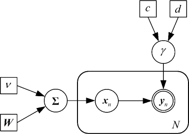
Figure 1: Proposed low-rank promoting hierarchical Gaussian prior model

II Bayesian Modeling

In the presence of noise, the canonical form of the matrix completion problem can be formulated as

$$\min_{\boldsymbol{X}}\quad \text{rank}(\boldsymbol{X})$$

s.t. $$\boldsymbol{Y}=\boldsymbol{\Omega}\ast(\boldsymbol{X}+\boldsymbol{E})$$ (3)

where $\boldsymbol{E}$ denotes the additive noise, and $\boldsymbol{\Omega}\in\{0,1\}^{M\times N}$ is a binary matrix that indicates which entries are observed. Without loss of generality, we assume $M\leq N$. As indicated earlier, minimizing the rank of a matrix is an NP-hard problem. In this paper, we consider modeling the matrix completion problem within a Bayesian framework.

We assume entries of $\boldsymbol{E}$ are independent and identically distributed (i.i.d.) random variables following a Gaussian distribution with zero mean and variance $\gamma^{-1}$. To learn $\gamma$, a Gamma hyperprior is placed over $\gamma$, i.e.

$$p(\gamma)=\text{Gamma}(\gamma|a,b)=\Gamma(a)^{-1}b^{a}\gamma^{a-1}e^{-b\gamma}$$ (4)

where $\Gamma(a)=\int_{0}^{\infty}t^{a-1}e^{-t}dt$ is the Gamma function. The parameters $a$ and $b$ are set to small values, e.g. $10^{-8}$, which makes the Gamma distribution a non-informative prior.

To promote the low-rankness of $\boldsymbol{X}$, we propose a two-layer hierarchical Gaussian prior model (see Fig. 1). Specifically, in the first layer, the columns of $\boldsymbol{X}$ are assumed mutually independent and follow a common Gaussian distribution:

$$p(\boldsymbol{X}|\boldsymbol{\Sigma})=\prod\limits_{n=1}^{N}p(\boldsymbol{x}_{n}|\boldsymbol{\Sigma})=\prod\limits_{n=1}^{N}\mathcal{N}(\boldsymbol{x}_{n}|\boldsymbol{0},\boldsymbol{\Sigma}^{-1})$$ (5)

where $\boldsymbol{x}_{n}$ denotes the $n$th column of $\boldsymbol{X}$, and $\boldsymbol{\Sigma}\in\mathbb{R}^{M\times M}$ is the precision matrix. The second layer specifies a Wishart distribution as a hyperprior over the precision matrix $\boldsymbol{\Sigma}$:

$$p(\boldsymbol{\Sigma})\propto |\boldsymbol{\Sigma}|^{\frac{\nu-M-1}{2}}\exp(-\frac{1}{2}\text{tr}(\boldsymbol{W}^{-1}\boldsymbol{\Sigma}))$$ (6)

where $\nu$ and $\boldsymbol{W}\in\mathbb{R}^{M\times M}$ denote the degrees of freedom and the scale matrix of the Wishart distribution, respectively. Note that the constraint $\nu>M-1$ for the standard Wishart distribution can be relaxed to $\nu>0$ if an improper prior is allowed, e.g. [26]. In Bayesian inference, improper prior distributes can often be used provided that the corresponding posterior distribution can be correctly normalized [27].

The Gaussian-inverse Wishart prior has the potential to encourage a low-rank solution. To illustrate this low-rankness promoting property, we integrate out the precision matrix $\boldsymbol{\Sigma}$ and obtain the marginal distribution of $\boldsymbol{X}$ as (details of the derivation can be found in Appendix A)

$$p(\boldsymbol{X})= \int\prod\limits_{n=1}^{N}p(\boldsymbol{x}_{n}|\boldsymbol{\Sigma})p(\boldsymbol{\Sigma})d\boldsymbol{\Sigma}$$

$$\propto |\boldsymbol{W}^{-1}+\boldsymbol{X}\boldsymbol{X}^{T}|^{-\frac{\nu+N}{2}}$$ (7)

From (7), we have

$$\log p(\boldsymbol{X})\propto-\log|\boldsymbol{X}\boldsymbol{X}^{T}+\boldsymbol{W}^{-1}|$$ (8)

If we choose $\boldsymbol{W}=\epsilon^{-1}\boldsymbol{I}$, and let $\epsilon$ be a small positive value, the log-marginal distribution becomes

$$\log p(\boldsymbol{X})\propto -\log|\boldsymbol{X}\boldsymbol{X}^{T}+\epsilon\boldsymbol{I}|$$

$$= -\sum_{m=1}^{M}\log(\lambda_{m}+\epsilon)$$ (9)

where $\lambda_{m}$ denotes the $m$th eigenvalue of $\boldsymbol{X}\boldsymbol{X}^{T}$. Clearly, in this case, the prior $p(\boldsymbol{X})$ encourages a low-rank solution $\boldsymbol{X}$. This is because maximizing the prior distribution $p(\boldsymbol{X})$ is equivalent to minimizing $\sum_{m=1}^{M}\log(\lambda_{m}+\epsilon)$ with respect to $\{\lambda_{m}\}$. It is well known that the log-sum function $\sum_{m=1}^{M}\log(\lambda_{m}+\epsilon)$ is an effective sparsity-promoting functional which encourages a sparse solution of $\{\lambda_{m}\}$ [28, 29, 30]. As a result, the resulting matrix $\boldsymbol{X}$ has a low-rank structure.

In addition to $\boldsymbol{W}=\epsilon^{-1}\boldsymbol{I}$, the parameter $\boldsymbol{W}$ can otherwise be devised in order to exploit additional prior knowledge about $\boldsymbol{X}$. For example, in some applications such as image inpainting, there is a spatial correlation among neighboring coefficients of $\boldsymbol{x}_{n}$. To capture the smoothness between neighboring coefficients, $\boldsymbol{W}$ can be set as [31]

$$\boldsymbol{W}=\boldsymbol{F}^{T}\boldsymbol{F}$$ (10)

where $\boldsymbol{F}\in\mathbb{R}^{M\times M}$ is a second-order difference operator with its $(i,j)$th entry given by

$$f_{i,j}=\begin{cases}-2,\quad&i=j\\ 1,&|i-j|=1\\ 0,&\text{else}\end{cases}$$ (11)

Another choice of $\boldsymbol{W}$ to promote a smooth solution is the Laplacian matrix [32], i.e.

$$\boldsymbol{W}=\boldsymbol{D}-\boldsymbol{A}+\hat{\epsilon}\boldsymbol{I}$$ (12)

where $\boldsymbol{A}$ is the adjacency matrix of a graph with its entries given by

$$a_{ij}=\exp\left(-\frac{|i-j|^{2}}{\theta^{2}}\right)$$ (13)

$\boldsymbol{D}$, referred to as the degree matrix, is a diagonal matrix with $d_{ii}=\sum_{j}a_{ij}$, and $\hat{\epsilon}$ is a small positive value to ensure $\boldsymbol{W}$ to be full rank.

It can be shown that $\boldsymbol{W}$ defined in (10) and (12) promotes low-rankness as well as smoothness of $\boldsymbol{X}$. To illustrate this, we first introduce the following lemma.

Lemma 1

For a positive-definite matrix $\boldsymbol{W}\in\mathbb{R}^{M\times M}$, the following equality holds valid

$$\log|\boldsymbol{X}\boldsymbol{X}^{T}+\boldsymbol{W}^{-1}|=\log|\boldsymbol{W}^{-1}|+\log|\boldsymbol{I}+\boldsymbol{X}^{T}\boldsymbol{W}\boldsymbol{X}|$$ (14)

for any $\boldsymbol{X}\in\mathbb{R}^{M\times N}$.

Proof:

See Appendix B. ∎

From Lemma 1, we have

$$\log p(\boldsymbol{X})\propto -\log|\boldsymbol{X}\boldsymbol{X}^{T}+\boldsymbol{W}^{-1}|$$

$$\propto -\log|\boldsymbol{I}+\boldsymbol{X}^{T}\boldsymbol{W}\boldsymbol{X}|$$

$$= -\sum_{n=1}^{N}\log(\tilde{\lambda}_{n}+1)$$ (15)

where $\tilde{\lambda}_{n}$ is the $n$th eigenvalue associated with $\boldsymbol{X}^{T}\boldsymbol{W}\boldsymbol{X}$. We see that maximizing the prior distribution is equivalent to minimizing $\sum_{n=1}^{N}\log(\tilde{\lambda}_{n}+1)$ with respect to $\{\tilde{\lambda}_{n}\}$. As discussed earlier, this log-sum functional is a sparsity-promoting functional which encourages a sparse solution $\{\tilde{\lambda}_{n}\}$. As a result, the matrix $\boldsymbol{X}^{T}\boldsymbol{W}\boldsymbol{X}$ has a low rank. Since $\boldsymbol{W}$ is full rank, this implies that $\boldsymbol{X}$ has a low-rank structure. On the other hand, notice that $\text{tr}(\boldsymbol{X}^{T}\boldsymbol{W}\boldsymbol{X})$ is the first-order approximation of $\log|\boldsymbol{I}+\boldsymbol{X}^{T}\boldsymbol{W}\boldsymbol{X}|$. Therefore minimizing $\log|\boldsymbol{I}+\boldsymbol{X}^{T}\boldsymbol{W}\boldsymbol{X}|$ will reduce the value of $\text{tr}(\boldsymbol{X}^{T}\boldsymbol{W}\boldsymbol{X})$. Clearly, for $\boldsymbol{W}$ defined in (10) and (12), a smoother solution results in a smaller value of $\text{tr}(\boldsymbol{X}^{T}\boldsymbol{W}\boldsymbol{X})$. Therefore when $\boldsymbol{W}$ is chosen to be (10) or (12), the resulting prior distribution $p(\boldsymbol{X})$ has the potential to encourage a low-rank and smooth solution.

Remarks: Our proposed hierarchical Gaussian prior model can be considered as a generalization of the prior model in [24]. Notice that in [24], the precision matrix in the prior model is assumed to be a deterministic parameter, whereas it is treated as a random variable and assigned a Wishart prior distribution in our model. This generalization offers more flexibility in modeling the underlying latent matrix. As discussed earlier, the parameter $\boldsymbol{W}$ can be devised to capture additional prior knowledge about the latent matrix, and such a careful choice of $\boldsymbol{W}$ can help substantially improve the recovery performance, as corroborated by our experimental results.

III Variational Bayesian Inference

III-A Review of The Variational Bayesian Methodology

Before proceeding, we firstly provide a brief review of the variational Bayesian (VB) methodology. In a probabilistic model, let $\boldsymbol{y}$ and $\boldsymbol{\theta}$ denote the observed data and the hidden variables, respectively. It is straightforward to show that the marginal probability of the observed data can be decomposed into two terms [27]

$$\ln p(\boldsymbol{y})=L(q)+\text{KL}(q||p),$$ (16)

where

$$L(q)=\int q(\boldsymbol{\theta})\ln\frac{p(\boldsymbol{y},\boldsymbol{\theta})}{q(\boldsymbol{\theta})}d\boldsymbol{\theta}$$ (17)

and

$$\text{KL}(q||p)=-\int q(\boldsymbol{\theta})\ln\frac{p(\boldsymbol{\theta}|\boldsymbol{y})}{q(\boldsymbol{\theta})}d\boldsymbol{\theta},$$ (18)

where $q(\boldsymbol{\theta})$ is any probability density function, $\text{KL}(q||p)$ is the Kullback-Leibler divergence [33] between $p(\boldsymbol{\theta}|\boldsymbol{y})$ and $q(\boldsymbol{\theta})$. Since $\text{KL}(q||p)\geq 0$, it follows that $L(q)$ is a rigorous lower bound for $\ln p(\boldsymbol{y})$. Moreover, notice that the left hand side of (16) is independent of $q(\boldsymbol{\theta})$. Therefore maximizing $L(q)$ is equivalent to minimizing $\text{KL}(q||p)$, and thus the posterior distribution $p(\boldsymbol{\theta}|\boldsymbol{y})$ can be approximated by $q(\boldsymbol{\theta})$ through maximizing $L(q)$.

The significance of the above transformation is that it circumvents the difficulty of computing the posterior probability $p(\boldsymbol{\theta}|\boldsymbol{y})$, when it is computationally intractable. For a suitable choice for the distribution $q(\boldsymbol{\theta})$, the quantity $L(q)$ may be more amiable to compute. Specifically, we could assume some specific parameterized functional form for $q(\boldsymbol{\theta})$ and then maximize $L(q)$ with respect to the parameters of the distribution. A particular form of $q(\boldsymbol{\theta})$ that has been widely used with great success is the factorized form over the component variables $\{\theta_{i}\}$ in $\boldsymbol{\theta}$ [34], i.e. $q(\boldsymbol{\theta})=\prod_{i}q_{i}(\theta_{i})$. We therefore can compute the posterior distribution approximation by finding $q(\boldsymbol{\theta})$ of the factorized form that maximizes the lower bound $L(q)$. The maximization can be conducted in an alternating fashion for each latent variable, which leads to [34]

$$q_{i}(\theta_{i})=\frac{e^{\langle\ln p(\boldsymbol{y},\boldsymbol{\theta})\rangle_{k\neq i}}}{\int e^{\langle\ln p(\boldsymbol{y},\boldsymbol{\theta})\rangle_{k\neq i}}d\theta_{i}},$$ (19)

where $\langle\cdot\rangle_{k\neq i}$ denotes the expectation with respect to the distributions $q_{k}(\theta_{k})$ for all $k\neq i$. By taking the logarithm on both sides of (19), it can be equivalently written as

$$\ln q_{i}(\theta_{i})=\langle\ln p(\boldsymbol{y},\boldsymbol{\theta})\rangle_{k\neq i}+\text{constant}.$$ (20)

III-B Proposed Algorithm

We now proceed to perform variational Bayesian inference for the proposed hierarchical model. Let $\boldsymbol{\theta}\triangleq\{\boldsymbol{X},\boldsymbol{\Sigma},\gamma\}$ denote all hidden variables. Our objective is to find the posterior distribution $p(\boldsymbol{\theta}|\boldsymbol{y})$. Since $p(\boldsymbol{\theta}|\boldsymbol{y})$ is usually computationally intractable, we, following the idea of [34], approximate $p(\boldsymbol{\theta}|\boldsymbol{y})$ as $q(\boldsymbol{X},\boldsymbol{\Sigma},\gamma)$ which has a factorized form over the hidden variables $\{\boldsymbol{X},\boldsymbol{\Sigma},\gamma\}$, i.e.

$$q(\boldsymbol{X},\boldsymbol{\Sigma},\gamma)=q_{x}(\boldsymbol{X})q_{\Sigma}(\boldsymbol{\Sigma})q_{\gamma}(\gamma).$$ (21)

As mentioned in the previous subsection, the maximization of $L(q)$ can be conducted in an alternating fashion for each latent variable, which leads to (details of the derivation can be found in [34])

$$\ln q_{x}(\boldsymbol{X})= \langle\ln p(\boldsymbol{\Sigma},\gamma)\rangle_{q_{\Sigma}(\boldsymbol{\Sigma})q_{\gamma}(\gamma)}+\text{constant},$$

$$\ln q_{\Sigma}(\boldsymbol{\Sigma})= \langle\ln p(\boldsymbol{X},\gamma)\rangle_{q_{x}(\boldsymbol{X})q_{\gamma}(\gamma)}+\text{constant},$$

$$\ln q_{\gamma}(\gamma)= \langle\ln p(\boldsymbol{X},\boldsymbol{\Sigma},)\rangle_{q_{x}(\boldsymbol{X})q_{\Sigma}(\boldsymbol{\Sigma})}+\text{constant},$$

where $\langle\rangle_{q_{1}(\cdot)\ldots q_{K}(\cdot)}$ denotes the expectation with respect to (w.r.t.) the distributions $\{q_{k}(\cdot)\}_{k=1}^{K}$. Details of this Bayesian inference scheme are provided next.

1). Update of $q_{x}(\boldsymbol{X})$: The calculation of $q_{x}(\boldsymbol{X})$ can be decomposed into a set of independent tasks, with each task computing the posterior distribution approximation for each column of $\boldsymbol{X}$, i.e. $q_{x}(\boldsymbol{x}_{n})$. We have

$$\ln q_{x}(\boldsymbol{x}_{n}) \propto\langle\ln[p(\boldsymbol{y}_{n}|\boldsymbol{x}_{n})p(\boldsymbol{x}_{n}|\boldsymbol{\Sigma})]\rangle_{q_{\Sigma}(\boldsymbol{\Sigma})q_{\gamma}(\gamma)}$$

$$\propto\langle-\gamma(\boldsymbol{y}_{n}-\boldsymbol{x}_{n})^{T}\boldsymbol{O}_{n}(\boldsymbol{y}_{n}-\boldsymbol{x}_{n})-\boldsymbol{x}_{n}^{T}\boldsymbol{\Sigma}\boldsymbol{x}_{n}\rangle$$

$$\propto-\boldsymbol{x}_{n}^{T}(\langle\gamma\rangle\boldsymbol{O}_{n}+\langle\boldsymbol{\Sigma}\rangle)\boldsymbol{x}_{n}+2\langle\gamma\rangle\boldsymbol{x}_{n}^{T}\boldsymbol{O}_{n}\boldsymbol{y}_{n}$$ (22)

where $\boldsymbol{y}_{n}$ denotes the $n$th column of $\boldsymbol{Y}$ and $\boldsymbol{O}_{n}\triangleq\text{diag}(\boldsymbol{o}_{n})$, with $\boldsymbol{o}_{n}$ being the $n$th column of $\boldsymbol{\Omega}$. From (22), it can be seen that $\boldsymbol{x}_{n}$ follows a Gaussian distribution

$$q_{x}(\boldsymbol{x}_{n})=\mathcal{N}(\boldsymbol{x}_{n}|\boldsymbol{\mu}_{n},\boldsymbol{Q}_{n})$$ (23)

with $\boldsymbol{\mu}_{n}$ and $\boldsymbol{Q}_{n}$ given as

$$\boldsymbol{\mu}_{n} =\langle\gamma\rangle\boldsymbol{Q}_{n}\boldsymbol{O}_{n}\boldsymbol{y}_{n}$$ (24)

$$\boldsymbol{Q}_{n} =(\langle\gamma\rangle\boldsymbol{O}_{n}+\langle\boldsymbol{\Sigma}\rangle)^{-1}$$ (25)

We see that to calculate $q_{x}(\boldsymbol{x}_{n})$, we need to perform an inverse operation of an $M\times M$ matrix which involves a computational complexity of $\mathcal{O}(M^{3})$.

2). Update of $q_{\Sigma}(\boldsymbol{\Sigma})$: The approximate posterior $q_{\Sigma}(\boldsymbol{\Sigma})$ can be obtained as

$$\ln q_{\Sigma}(\boldsymbol{\Sigma})$$

$$\propto \langle\ln[\prod\limits_{n=1}^{N}p(\boldsymbol{x}_{n}|\boldsymbol{\Sigma})p(\boldsymbol{\Sigma})]\rangle_{q_{x}(\boldsymbol{X})}$$

$$\propto \langle\frac{N}{2}\ln|\boldsymbol{\Sigma}|-\frac{1}{2}\text{tr}(\boldsymbol{X}^{T}\boldsymbol{\Sigma}\boldsymbol{X})+\frac{\nu-M-1}{2}\ln|\boldsymbol{\Sigma}|$$

$$-\frac{1}{2}\text{tr}(\boldsymbol{W}^{-1}\boldsymbol{\Sigma})\rangle$$

$$\propto \frac{\nu+N-M-1}{2}\ln|\boldsymbol{\Sigma}|-\frac{1}{2}\text{tr}((\boldsymbol{W}^{-1}+\langle\boldsymbol{X}\boldsymbol{X}^{T}\rangle)\boldsymbol{\Sigma})$$ (26)

From (26), it can be seen that $\boldsymbol{\Sigma}$ follows a Wishart distribution, i.e.

$$q_{\Sigma}(\boldsymbol{\Sigma})=\text{Wishart}(\boldsymbol{\Sigma};\hat{\boldsymbol{W}},\hat{\nu})$$ (27)

where

$$\hat{\boldsymbol{W}} =(\boldsymbol{W}^{-1}+\langle\boldsymbol{X}\boldsymbol{X}^{T}\rangle)^{-1}$$ (28)

$$\hat{\nu} =\nu+N$$ (29)

3). Update of $q_{\gamma}(\boldsymbol{\gamma})$: The variational optimization of $q_{\gamma}(\gamma)$ yields

$$\ln q_{\gamma}(\gamma)\propto \langle\ln p(\boldsymbol{Y}|\boldsymbol{X},\gamma)p(\gamma)\rangle_{q_{x}(\boldsymbol{X})}$$

$$\propto \langle\ln\prod_{(m,n)\in\mathbb{S}}p(y_{mn}|x_{mn},\gamma)p(\gamma)\rangle$$

$$\propto \langle\frac{L}{2}\ln\gamma-\frac{\gamma}{2}\sum_{(m,n)\in\mathbb{S}}(y_{mn}-x_{mn})^{2}+(c-1)\ln\gamma-d\gamma\rangle$$

$$= \bigg{(}\frac{L}{2}+c-1\bigg{)}\ln\gamma-\bigg{(}\frac{1}{2}\sum_{(m,n)\in\mathbb{S}}\langle(y_{mn}-x_{mn})^{2}\rangle+d\bigg{)}\gamma$$ (30)

where $x_{mn}$ and $y_{mn}$ denote the $(m,n)$th entry of $\boldsymbol{X}$ and $\boldsymbol{Y}$, respectively, $\mathbb{S}\triangleq\{(m,n)|\Omega_{mn}=1\}$ is an index set consisting of indices of those observed entries, and $L\triangleq|\mathbb{S}|$ is the cardinality of the set $\mathbb{S}$, in which $\Omega_{mn}$ denotes the $(m,n)$th entry of $\boldsymbol{\Omega}$.

It is easy to verify that $q_{\gamma}(\gamma)$ follows a Gamma distribution

$$q_{\gamma}(\gamma)=\text{Gamma}(\gamma|\tilde{c},\tilde{d})$$ (31)

with the parameters $\tilde{c}$ and $\tilde{d}$ given respectively by

$$\tilde{c}= \frac{L}{2}+c,$$

$$\tilde{d}= \frac{1}{2}\sum_{(m,n)\in\mathbb{S}}\langle(y_{mn}-x_{mn})^{2}\rangle+d$$ (32)

where

$$\langle(y_{mn}-x_{mn})^{2}\rangle=y_{mn}^{2}-2y_{mn}\langle x_{mn}\rangle+\langle x_{mn}^{2}\rangle$$ (33)

Some of the expectations and moments used during the update are summarized as

$$\langle\boldsymbol{\Sigma}\rangle =\hat{\boldsymbol{W}}\hat{\nu}$$ (34)

$$\langle\boldsymbol{X}\boldsymbol{X}^{T}\rangle =\langle\boldsymbol{X}\rangle\langle\boldsymbol{X}\rangle^{T}+\sum\limits_{n=1}^{N}\boldsymbol{Q}_{n}$$ (35)

$$\langle x_{mn}^{2}\rangle =\langle x_{mn}\rangle^{2}+Q_{n}(m,m)$$ (36)

where $Q_{n}(m,m)$ denotes the $m$th diagonal entry of $\boldsymbol{Q}_{n}$.

For clarity, we summarize our algorithm as follows.

Algorithm 1 VB Algorithm for Matrix Completion

0:  $\boldsymbol{Y}$, $\boldsymbol{\Omega}$, $\nu$ and $\boldsymbol{W}$.

0:  $q_{x}(\boldsymbol{X})$, $q_{\Sigma}(\boldsymbol{\Sigma})$, $q_{\gamma}(\gamma)$.

  Initialize $\langle\boldsymbol{\Sigma}\rangle$ and $\langle\gamma\rangle$;

  while not converge do

     for $n=1$ to $N$ do

        Update $q_{x}({\boldsymbol{x}_{n}})$ via (23), with $q_{\Sigma}(\boldsymbol{\Sigma})$ and $q_{\gamma}(\gamma)$ fixed;

     end for

     Update $q_{\Sigma}({\boldsymbol{\Sigma}})$ via (27), with $q_{x}(\boldsymbol{X})$ and $q_{\gamma}(\gamma)$ fixed;

     Update $q_{\gamma}(\gamma)$ via (31);

  end while

It can be easily checked that the computational complexity of our proposed method is dominated by the update of the posterior distribution $q_{x}(\boldsymbol{X})$, which requires computing an $M\times M$ matrix inverse $N$ times and therefore has a computational complexity scaling as $\mathcal{O}(M^{3}N)$. This makes the application of our proposed method to large data sets impractical. To address this issue, in the following, we develop a computationally efficient algorithm which obtains an approximation of $q_{x}(\boldsymbol{X})$ by resorting to the generalized approximate message passing (GAMP) technique [35].

IV VB-GAMP

GAMP is a low-complexity Bayesian iterative technique recently developed in [36, 35] for obtaining approximate marginal posteriors. Note that the GAMP algorithm requires that both the prior distribution and the noise distribution have factorized forms [35]. Nevertheless, in our model, the prior distribution $p(\boldsymbol{x}_{n}|\boldsymbol{\Sigma})$ has a non-factorizable form, in which case the GAMP technique cannot be directly applied. To address this issue, we first construct a surrogate problem which aims to recover $\boldsymbol{x}\in\mathbb{R}^{M}$ from linear measurements $\boldsymbol{b}\in\mathbb{R}^{M}$:

$$\boldsymbol{b}=\boldsymbol{U}^{T}\boldsymbol{x}+\boldsymbol{e}$$ (37)

where $\boldsymbol{U}\in\mathbb{C}^{M\times M}$ is obtained by performing a singular value decomposition of $\langle\boldsymbol{\Sigma}\rangle=\boldsymbol{U}\boldsymbol{S}\boldsymbol{U}^{T}$, $\boldsymbol{U}$ is a unitary matrix and $\boldsymbol{S}$ is a diagonal matrix with its diagonal elements equal to the singular values of $\langle\boldsymbol{\Sigma}\rangle$, and $\boldsymbol{e}$ denotes the additive Gaussian noise with zero mean and covariance matrix $\boldsymbol{S}^{-1}$. We assume that entries of $\boldsymbol{x}$ are mutually independent and follow the following distribution:

$$p(x_{m})=\begin{cases}\mathcal{N}(\kappa_{m},\xi^{-1})&\text{if $\pi_{m}=1$}\\ C,&\text{if $\pi_{m}=0$}\end{cases}$$ (38)

where $\pi_{m}$, $x_{m}$, and $\kappa_{m}$ denote the $m$th entry of $\boldsymbol{\pi}$, $\boldsymbol{x}$, and $\boldsymbol{\kappa}$, respectively, $C$ is a constant, $\boldsymbol{\pi}$, $\boldsymbol{\kappa}\in\mathbb{R}^{M\times 1}$ and $\xi$ are known parameters. It is noted that although $p(x_{m})=C$ is an improper prior distribution, it can often be used provided the corresponding posterior distribution can be correctly normalized [27]. Considering the surrogate problem (37), the posterior distribution of $\boldsymbol{x}$ can be calculated as

$$p(\boldsymbol{x}|\boldsymbol{b}) \propto p(\boldsymbol{b}|\boldsymbol{x})p(\boldsymbol{x})$$

$$\propto p(\boldsymbol{b}|\boldsymbol{x})\prod_{m\in S}p(x_{m})$$

$$=\mathcal{N}(\boldsymbol{U}^{T}\boldsymbol{x},\boldsymbol{S}^{-1})\prod_{m\in S}\mathcal{N}(\kappa_{m},\xi^{-1})$$ (39)

where $S\triangleq\{m|\pi_{m}=1\}$.

Taking the logarithm of $p(\boldsymbol{x}|\boldsymbol{b})$, we have

$$\ln p(\boldsymbol{x}|\boldsymbol{b}) \propto-\frac{1}{2}(\boldsymbol{b}-\boldsymbol{U}^{T}\boldsymbol{x})^{T}\boldsymbol{S}(\boldsymbol{b}-\boldsymbol{U}^{T}\boldsymbol{x})$$

$$\quad-\frac{1}{2}\xi\sum_{m\in S}(x_{m}-\kappa_{m})^{2}$$

$$=-\frac{1}{2}(\boldsymbol{b}-\boldsymbol{U}^{T}\boldsymbol{x})^{T}\boldsymbol{S}(\boldsymbol{b}-\boldsymbol{U}^{T}\boldsymbol{x})$$

$$\quad-\frac{1}{2}\xi(\boldsymbol{x}-\boldsymbol{\kappa})^{T}\boldsymbol{\Pi}(\boldsymbol{x}-\boldsymbol{\kappa})$$

$$\propto-\frac{1}{2}\boldsymbol{x}^{T}(\boldsymbol{U}\boldsymbol{S}\boldsymbol{U}^{T}+\xi\boldsymbol{\Pi})\boldsymbol{x}^{T}+(\boldsymbol{b}^{T}\boldsymbol{S}\boldsymbol{U}^{T}+\xi\boldsymbol{\kappa}^{T}\boldsymbol{\Pi})\boldsymbol{x}$$ (40)

where $\boldsymbol{\Pi}$ is a diagonal matrix with its $m$th diagonal entry equal to $\pi_{m}$. Clearly, $p(\boldsymbol{x}|\boldsymbol{b})$ follows a Gaussian distribution with its mean $\boldsymbol{\mu}$ and covariance matrix $\boldsymbol{Q}$ given by

$$\boldsymbol{\mu}= \boldsymbol{Q}(\boldsymbol{U}\boldsymbol{S}\boldsymbol{b}+\xi\boldsymbol{\Pi}\boldsymbol{\kappa})$$ (41)

$$\boldsymbol{Q}= (\boldsymbol{U}\boldsymbol{S}\boldsymbol{U}^{T}+\xi\boldsymbol{\Pi})^{-1}=(\langle\boldsymbol{\Sigma}\rangle+\xi\boldsymbol{\Pi})^{-1}$$ (42)

Comparing (24)–(25) with (41)–(42), we can readily verify that when $\boldsymbol{b}=\boldsymbol{0}$, $\boldsymbol{\kappa}=\boldsymbol{y}_{n}$, $\boldsymbol{\pi}=\boldsymbol{o}_{n}$ (i.e. $\boldsymbol{\Pi}=\boldsymbol{O}_{n}$), and $\xi=\langle\gamma\rangle$, $p(\boldsymbol{x}|\boldsymbol{b})$ is exactly the desired posterior distribution $q_{x}(\boldsymbol{x}_{n})$. Meanwhile, notice that for the surrogate problem (37), both the prior distribution and the noise distribution are factorizable. Hence the GAMP algorithm can be directly applied to (37) to find an approximation of the posterior distribution $p(\boldsymbol{x}|\boldsymbol{b})$. By setting $\boldsymbol{b}=\boldsymbol{0}$, $\boldsymbol{\kappa}=\boldsymbol{y}_{n}$, $\boldsymbol{\pi}=\boldsymbol{o}_{n}$, $\xi=\langle\gamma\rangle$, an approximate of $q_{x}(\boldsymbol{x}_{n})$ in (23) can be efficiently obtained. We now proceed to derive the GAMP algorithm for the surrogate problem (37).

IV-A Solving (37) via GAMP

GAMP was developed in a message passing-based framework. By using central-limit-theorem approximations, message passing between variable nodes and factor nodes can be greatly simplified, and the loopy belief propagation on the underlying factor graph can be efficiently performed. As noted in [35], the central-limit-theorem approximations become exact in the large-system limit under an i.i.d. zero-mean sub-Gaussian measurement matrix.

Firstly, GAMP approximates the true marginal posterior distribution $p(x_{m}|\boldsymbol{b})$ by

$$\hat{p}(x_{m}|\boldsymbol{b},\hat{r}_{m},\tau_{m}^{r})= \frac{p(x_{m})\mathcal{N}(x_{m}|\hat{r}_{m},\tau_{m}^{r})}{\int_{x}p(x_{m})\mathcal{N}(x_{m}|\hat{r}_{m},\tau_{m}^{r})}$$ (43)

where $\hat{r}_{m}$ and $\tau_{m}^{r}$ are quantities iteratively updated during the iterative process of the GAMP algorithm. Here, we have dropped their explicit dependence on the iteration number $k$ for simplicity. For the case $\pi_{m}=1$, substituting the prior distribution (38) into (43), it can be easily verified that the approximate posterior $\hat{p}(x_{m}|\boldsymbol{b},\hat{r}_{m},\tau_{m}^{r})$ follows a Gaussian distribution with its mean and variance given respectively as

$$\mu_{m}^{x} =\phi_{m}^{x}(\xi\kappa_{m}+\hat{r}_{m}/\tau_{m}^{r})$$ (44)

$$\phi_{m}^{x} =\frac{\tau_{m}^{r}}{1+\xi\tau_{m}^{r}}$$ (45)

Similarly, for the case $\pi_{m}=0$, substituting the prior distribution (38) into (43), the approximate posterior $\hat{p}(x_{m}|\boldsymbol{b},\hat{r}_{m},\tau_{m}^{r})$ follows a Gaussian distribution with its mean and variance given respectively as

$$\mu_{m}^{x} =\hat{r}_{m}$$ (46)

$$\phi_{m}^{x} =\tau_{m}^{r}$$ (47)

Another approximation is made to the noiseless output $z_{i}\triangleq\boldsymbol{u}_{i}^{T}\boldsymbol{x}$, where $\boldsymbol{u}_{i}^{T}$ denotes the $i$th row of $\boldsymbol{U}^{T}$. GAMP approximates the true marginal posterior $p(z_{i}|\boldsymbol{b})$ by

$$\hat{p}(z_{i}|\boldsymbol{b},\hat{p}_{i},\tau_{i}^{p})=\frac{p(b_{i}|z_{i})\mathcal{N}(z_{i}|\hat{p}_{i},\tau_{i}^{p})}{\int_{z}p(b_{i}|z_{i})\mathcal{N}(z_{i}|\hat{p}_{i},\tau_{i}^{p})}$$ (48)

where $\hat{p}_{i}$ and $\tau_{i}^{p}$ are quantities iteratively updated during the iterative process of the GAMP algorithm. Again, here we dropped their explicit dependence on the iteration number $k$. Under the additive white Gaussian noise assumption, we have $p(b_{i}|z_{i})=\mathcal{N}(b_{i}|z_{i},s_{i}^{-1})$, where $s_{i}$ denotes the $i$th diagonal element of $\boldsymbol{S}$. Thus $\hat{p}(z_{i}|\boldsymbol{b},\hat{p}_{i},\tau_{i}^{p})$ also follows a Gaussian distribution with its mean and variance given by

$$\mu_{i}^{z}= \frac{\tau_{i}^{p}s_{i}b_{i}+\hat{p}_{i}}{1+s_{i}\tau_{i}^{p}}$$ (49)

$$\phi_{i}^{z}= \frac{\tau_{i}^{p}}{1+s_{i}\tau_{i}^{p}}$$ (50)

With the above approximations, we can now define the following two scalar functions: $g_{\text{in}}(\cdot)$ and $g_{\text{out}}(\cdot)$ that are used in the GAMP algorithm. The input scalar function $g_{\text{in}}(\cdot)$ is simply defined as the posterior mean $\mu_{m}^{x}$, i.e.

$$g_{\text{in}}(\hat{r}_{m},\tau_{m}^{r})=\mu_{m}^{x}=\begin{cases}\phi_{m}^{x}(\xi\kappa_{m}+\hat{r}_{m}/\tau_{m}^{r})&\text{if $\pi_{m}=1$}\\ \hat{r}_{m}&\text{if $\pi_{m}=0$}\end{cases}$$ (51)

The scaled partial derivative of $\tau_{m}^{r}g_{\text{in}}(\hat{r}_{m},\tau_{m}^{r})$ with respect to $\hat{r}_{m}$ is the posterior variance $\phi_{m}^{x}$, i.e.

$$\tau_{m}^{r}\frac{\partial}{\partial\hat{r}_{m}}g_{\text{in}}(\hat{r}_{m},\tau_{m}^{r})=\phi_{m}^{x}=\begin{cases}\frac{\tau_{m}^{r}}{1+\xi\tau_{m}^{r}}&\text{if $\pi_{m}=1$}\\ \tau_{m}^{r}&\text{if $\pi_{m}=0$}\end{cases}$$ (52)

The output scalar function $g_{\text{out}}(\cdot)$ is related to the posterior mean $\mu_{i}^{z}$ as follows

$$g_{\text{out}}(\hat{p}_{i},\tau_{i,n}^{p}) =\frac{1}{\tau_{i}^{p}}(\mu_{i}^{z}-\hat{p}_{i})=\frac{s_{i}(b_{i}-\hat{p}_{i})}{1+s_{i}\tau_{i}^{p}}$$ (53)

The partial derivative of $g_{\text{out}}(\hat{p}_{i},\tau_{i}^{p})$ is related to the posterior variance $\phi_{i,n}^{z}$ in the following way

$$\frac{\partial}{\partial\hat{p}_{i}}g_{\text{out}}(\hat{p}_{i},\tau_{i}^{p})=\frac{\phi_{i}^{z}-\tau_{i}^{p}}{(\tau_{i}^{p})^{2}}=\frac{-s_{i}}{(1+s_{i}\tau_{i}^{p})}$$ (54)

Given the above definitions of $g_{\text{in}}(\cdot)$ and $g_{\text{out}}(\cdot)$, the GAMP algorithm tailored to the considered problem (37) can now be summarized as follows (details of the derivation of the GAMP algorithm can be found in [35]), in which $u_{i,m}$ denotes the $(i,m)$th entry of $\boldsymbol{U}^{T}$.

Algorithm 2 GAMP Algorithm

0:  $\boldsymbol{\kappa}$, $\boldsymbol{\pi}$, $\boldsymbol{b}$, and $\xi$.

0:  $\{\hat{r}_{m},\tau_{m}^{r}\}$, $\{\hat{p}_{i},\tau_{i}^{p}\}$, and $\{\mu_{m}^{x},\phi_{m}^{x}\}$.

  Initialization: Set $\hat{\psi}_{i}=0,\forall i\in\{1,\ldots,M\}$; $\{\mu_{m}^{x}\}_{m=1}^{M}$ are initialized as the mean variance of the prior distribution, and $\{\phi_{m}^{x}\}_{m=1}^{M}$ are set to small values, say $10^{-5}$.

  while not converge do

     Step 1. $\forall i\in\{1,\ldots,M\}$: $\begin{aligned} \qquad\qquad\quad\hat{z}_{i}=&\sum_{m}u_{i,m}\mu_{m}^{x}\\ \tau_{i}^{p}=&\sum_{m}u_{i,m}^{2}\phi_{m}^{x}\\ \hat{p}_{i}=&\hat{z}_{i}-\tau_{i}^{p}\hat{\psi}_{i}\\ \end{aligned}$

     Step 2. $\forall i\in\{1,\ldots,M\}$: $\begin{aligned} \qquad\qquad\quad\hat{\psi}_{i}=&g_{\text{out}}(\hat{p}_{i},\tau^{p}_{i})\\ \tau^{s}_{i}=&-\frac{\partial}{\partial\hat{p}_{i}}g_{\text{out}}(\hat{p}_{i},\tau^{p}_{i})\\ \end{aligned}$

     Step 3. $\forall m\in\{1,\ldots,M\}$: $\begin{aligned} \qquad\qquad\quad\tau_{m}^{r}=&\left(\sum_{i}u_{i,m}^{2}\tau^{s}_{i}\right)^{-1}\\ \hat{r}_{m}=&\mu_{m}^{x}+\tau_{m}^{r}\sum_{i}u_{i,m}\hat{\psi}_{i}\\ \end{aligned}$

     Step 4. $\forall m\in\{1,\ldots,M\}$: $\begin{aligned} \qquad\qquad\quad\mu_{m}^{x}=&g_{\text{in}}(\hat{r}_{m},\tau_{m}^{r})\\ \phi_{m}^{x}=&\tau_{m}^{r}\frac{\partial}{\partial\hat{r}_{m}}g_{\text{in}}(\hat{r}_{m},\tau_{m}^{r})\\ \end{aligned}$

  end while

IV-B Discussions

We have now derived an efficient algorithm to obtain an approximate posterior distribution of $\boldsymbol{x}$ for (37). Specifically, the true marginal posterior distribution of $x_{m}$ is approximated by a Gaussian distribution $\hat{p}(x_{m}|\boldsymbol{b},\hat{r}_{m},\tau_{m}^{r})$ with its mean and variance given by (44)–(45) or (46)–(47), depending on the value of $\pi_{m}$. The joint posterior distribution $p(\boldsymbol{x}|\boldsymbol{b})$ can be approximated as a product of approximate marginal posterior distributions:

$$p(\boldsymbol{x}|\boldsymbol{b})\approx\hat{p}(\boldsymbol{x}|\boldsymbol{b})=\prod\limits_{m=1}^{M}\hat{p}(x_{m}|\boldsymbol{b},\hat{r}_{m},\tau_{m}^{r})$$ (55)

As indicated earlier, by setting $\boldsymbol{b}=\boldsymbol{0}$, $\boldsymbol{\kappa}=\boldsymbol{y}_{n}$, $\boldsymbol{\pi}=\boldsymbol{o}_{n}$, and $\xi=\langle\gamma\rangle$, the posterior distribution $\hat{p}(\boldsymbol{x}|\boldsymbol{b})$ obtained via the GAMP algorithm can be used to approximate $q_{x}(\boldsymbol{x}_{n})$ in (23).

We see that to approximate $q_{x}(\boldsymbol{X})$ by using the GAMP, we first need to perform a singular value decomposition (SVD) of $\langle\boldsymbol{\Sigma}\rangle$, which has a computational complexity of $\mathcal{O}(M^{3})$. The GAMP algorithm used to approximate $q_{x}(\boldsymbol{x}_{n})$ involves very simple matrix-vector multiplications which has a computational complexity scaling as $\mathcal{O}(M^{2})$. Therefore the overall computational complexity for updating $q_{x}(\boldsymbol{X})$ is of order $\mathcal{O}(M^{2}N+M^{3})$. In contrast, using (24)–(25) to update $q_{x}(\boldsymbol{X})$ requires a computational complexity of $\mathcal{O}(NM^{3})$. Thus the GAMP technique can help achieve a significant reduction in the computational complexity as compared with a direct calculation of $q_{x}(\boldsymbol{X})$.

For clarity, the VB-GAMP algorithm for matrix completion is summarized as

Algorithm 3 VB-GAMP Algorithm for Matrix Completion

0:  $\boldsymbol{Y}$, $\boldsymbol{\Omega}$, $\nu$ and $\boldsymbol{W}$.

0:  $q_{x}(\boldsymbol{X})$, $q_{\Sigma}(\boldsymbol{\Sigma})$, and $q_{\gamma}(\gamma)$.

1:  Initialize $\langle\boldsymbol{X}\rangle$, $\langle\boldsymbol{\Sigma}\rangle$;

2:  while not converge do

3:     Calculate singular value decomposition of $\langle\boldsymbol{\Sigma}\rangle$;

4:     for $n=1$ to $N$ do

5:        Obtain an approximation of $q_{x}(\boldsymbol{x}_{n})$ via Algorithm 2;

6:     end for

7:     Update $q_{\Sigma}({\boldsymbol{\Sigma}})$ via (27);

8:     Update $q_{\gamma}(\gamma)$ via (31);

9:  end while

The proposed method proceeds in a double-loop manner, the outer loop calculate the variational posterior distributions $q_{\gamma}(\gamma)$ and $q_{\Sigma}(\boldsymbol{\Sigma})$, and the inner loop computes an approximation of $q_{x}(\boldsymbol{X})$. It is noted that there is no need to wait until the GAMP converges. Experimental results show that GAMP provides a reliable approximation of $q_{x}(\boldsymbol{x}_{n})$ even if only a few iterations are performed. In our experiments, only one iteration is used to implement GAMP.

V Experiments

In this section, we carry out experiments to illustrate the performance of our proposed GAMP-assisted Bayesian matrix completion method with hierarchical Gaussian priors (referred to as BMC-GP-GAMP). Throughout our experiments, the parameters used in our method are set to be $a=b=10^{-10}$ and $\nu=1$. Here we choose a small $\nu$ in order to encourage a low-rank precision matrix. We compare our method with several state-of-the-art methods, namely, the variational sparse Bayesian learning method (also referred to as VSBL) [20] which models the low-rankness of the matrix as the structural sparsity of its two factor matrices, the bilinear GAMP-based matrix completion method (also referred to as BiGAMP-MC) [23] which implements the VSBL using bilinear GAMP, the inexact version of the augmented Lagrange multiplier based matrix completion method (also referred to ALM-MC) [15], and a low-rank matrix fitting method (also referred to as LMaFit) [37] which iteratively minimizes the fitting error and estimates the rank of the matrix. It should be noted that both VSBL and LMaFit require to set an over-estimated rank. Note that we did not include [24] in our experiments due to its prohibitive computational complexity when the matrix dimension is large. Codes of our proposed algorithm along with other competing algorithms are available at http://www.junfang-uestc.net/codes/LRMC.rar, in which codes of other competing algorithms are obtained from their respective websites.

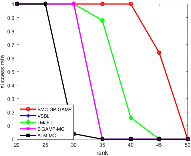
(a)

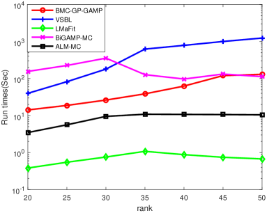
(b)

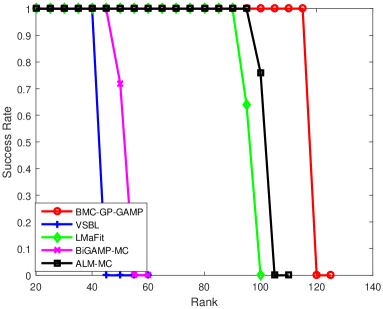
(c)

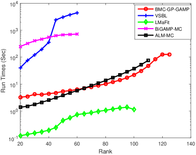
(d)

Figure 2: Synthetic data: (a) Success rates vs. the rank of the matrix, $\rho=0.2$; (b) Run times vs. the rank of the matrix, $\rho=0.2$; (c) Success rates vs. the rank of the matrix $\rho=0.5$; (d) Run times vs. the rank of the matrix, $\rho=0.5$

V-A Synthetic data

We first examine the effectiveness of our proposed method on synthetic data. We generate the test rank-$k$ matrix $\boldsymbol{X}$ of size $500\times 500$ by multiplying $\boldsymbol{A}\in\mathbb{R}^{500\times k}$ by the transpose of $\boldsymbol{B}\in\mathbb{R}^{500\times k}$, i.e. $\boldsymbol{X}=\boldsymbol{A}\boldsymbol{B}^{T}$. All the entries of $\boldsymbol{A}$ and $\boldsymbol{B}$ are sampled from a normal distribution. We consider the scenarios where $20\%$ ($\rho=0.2$) and $50\%$ ($\rho=0.5$) entries of $\boldsymbol{X}$ are observed. Here $\rho$ denotes the sampling ratio. The success rates as well as the run times of respective algorithms as a function of the rank of $\boldsymbol{X}$, i.e. $k$, are plotted in Fig. 2 Results are averaged over 25 independent trials. A trial is considered to be successful if the relative error is smaller than $10^{-2}$, i.e. $||\boldsymbol{X}-\boldsymbol{\hat{X}}||_{F}/||\boldsymbol{X}||_{F}<10^{-2}$, where $\boldsymbol{\hat{X}}$ denotes the estimated matrix. For our proposed method, the matrix parameter $\boldsymbol{W}$ is set to $10^{10}\boldsymbol{I}$. The pre-defined overestimated rank for VSBL and LMaFit is set to be twice the true rank. For the case $\rho=0.2$, VSBL and BiGAMP-MC present the same recovery performance with their curves overlapping each other. From Fig. 2, we can see that

• Our proposed method presents the best performance for both sampling ratio cases. Meanwhile, it has a moderate computational complexity. When the sampling ratio is set to 0.5, our proposed method has a run time similar to the ALM-MC method, while provides a clear performance improvement over the ALM-MC.

• The LMaFit method is the most computationally efficient. But its performance is not as good as our proposed method.

• The proposed method outperforms the other two Bayesian methods, namely, the VSBL and the BiGAMP-MC, by a big margin in terms of both recovery accuracy and computational complexity. Since the BiGAMP cannot automatically determine the matrix rank, it needs to try all possible values of the rank, which makes running the BiGAMP-MC time costly.

TABLE I: Error Rate for Chr22 Dataset

	$20\%$	$50\%$
BMC-GP-GAMP	0.0567	0.0233
VSBL	0.0587	0.0249
LMaFit	0.2525	0.2472
BiGAMP-MC	0.0573	0.0282
ALM-MC	0.0550	0.0246

V-B Gene data

We carry out experiments on gene data for genotype estimation. The dataset [4] is a matrix of size $790\times 112$ provided by Wellcome Trust Case Control Consortium (WTCCC) and contains the genetic information from chromosome 22. The dataset, which is referred to as “Chr22”, has been shown in [4] to be approximately low-rank. We randomly select $20\%$ or $50\%$ of the entries of the dataset as observations, and recover the rest entries using low-rank matrix completion methods. Again, for our proposed method, the matrix parameter $\boldsymbol{W}$ is set to $10^{10}\boldsymbol{I}$. The pre-defined ranks used for VSBL and LMaFit are both set to $100$. Following [4], we use a metric termed as “allelic-imputation error rate” to evaluate the performance of respective methods. The error rate is defined as

$$\text{Error Rate}=\frac{\text{nnz}(|\boldsymbol{X}-\text{round}(\hat{\boldsymbol{X}})|)}{T}$$ (56)

where $\boldsymbol{X}$ and $\hat{\boldsymbol{X}}$ denotes the true and the estimated matrices, respectively, the operation $\text{round}(\boldsymbol{X})$ returns a matrix with each entry of $\boldsymbol{X}$ rounded to its nearest integer, $\text{nnz}(\boldsymbol{X})$ counts the number of non-zero entries of $\boldsymbol{X}$, and $T$ denotes the number of unobserved entries. We report the average error rates of respective algorithms in Table I. From Table I, we see that all methods, except the LMaFit method, present similar results and the proposed method slightly outperforms other methods when $50\%$ entries are observed. Despite the superior performance on synthetic data, the LMaFit method incurs large estimation errors for this dataset.

TABLE II: NMAE for 100k Movielens Dataset

	$20\%$	$50\%$
BMC-GP-GAMP	0.1931	0.1851
VSBL	0.2004	0.1847
LMaFit	0.2677	0.2354
BiGAMP-MC	0.2009	0.1856
ALM-MC	0.2002	0.1893

V-C Collaborative Filtering

In this experiment, we study the performance of respective methods on the task of collaborative filtering. We use the MovieLens 100k dataset, which consists of $10^{5}$ ratings ranging from 1 to 5 on 1682 movies from 943 users. The ratings can form a matrix of size $943\times 1682$. We randomly choose $20\%$ or $50\%$ of available ratings as training data, and predict the rest ratings using respective matrix completion methods. The matrix parameter $\boldsymbol{W}$ used in the proposed method is set to $10^{10}\boldsymbol{I}$. The pre-defined ranks used for VSBL and LMaFit are both set to $100$. The performance is evaluated by the normalized mean absolute error (NMAE), which is calculated as

$$\text{NMAE}=\frac{\sum_{(i,j)\in S}|x_{ij}-\hat{x}_{ij}|}{(r_{\text{max}}-r_{\text{min}})|S|}$$ (57)

where $S$ is a set containing the indexes of those unobserved available ratings, $r_{\text{max}}$ and $r_{\text{min}}$ denote the maximum and minimum ratings, respectively. The results of NMAE are shown in Table II, from which we see that the proposed method achieves the most accurate rating prediction when the number of observed ratings is small.

TABLE III: Image Inpainting (PSNR/SSIM)

	Monarch		Lena
	$30\%$	$50\%$	$20\%$	$30\%$
BMC-GP-GAMP-I	19.3328/0.4942	23.8965/0.7066	23.4235/0.4946	25.6866/0.5991
BMC-GP-GAMP-II	20.8628/0.6960	25.6955/0.8705	25.3337/0.7479	28.0434/0.8328
BMC-GP-GAMP-III	21.1797/0.6710	25.6665/0.8422	25.2876/0.7388	27.9684/0.8213
VSBL	16.5478/0.3625	19.9965/0.5468	21.5168/0.4999	23.8180/0.5964
LMaFit	17.6527/0.4018	19.2834/0.5117	21.5525/0.4494	22.3862/0.5504
BiGAMP-MC	18.9154/0.4618	22.3883/0.6338	22.6557/0.4869	24.8173/0.5997
ALM-MC	19.6250/0.5149	23.6854/0.7253	23.1028/0.5164	25.5310/0.6433

V-D Image Inpainting

Lastly, we evaluate the performance of different methods on image inpainting. The objective of image inpainting is to complete an image with missing pixels. We conduct experiments on the benchmark images Butterfly and Lena, which are of size $256\times 256$ and $512\times 512$, respectively. In our experiments, we examine the performance of our proposed method under different choices of $\boldsymbol{W}$. As usual, we can set $\boldsymbol{W}=10^{10}\boldsymbol{I}$. Such a choice of $\boldsymbol{W}$ is referred to as BMC-GP-GAMP-I. We can also set $\boldsymbol{W}$ according to (10) and (12), which are respectively referred to as BMC-GP-GAMP-II and BMC-GP-GAMP-III. The parameters $\hat{\epsilon}$ and $\theta$ in (12) are set to $10^{-6}$ and $\sqrt{3}$, respectively. As discussed earlier in our paper, the latter two choices exploit both the low-rankness and the smoothness of the signal. For the Butterfly image, we consider cases where $30\%$ and $50\%$ of pixels in the image are observed. For the Lena image, we consider cases where $20\%$ and $40\%$ of pixels are observed. We report the peak signal to noise ratio (PSNR) as well as the structural similarity (SSIM) index of each algorithm in Table III. The original image with missing pixels and these images reconstructed by respective algorithms are shown in Fig. 3, 4, 5, and 6. From Table III, we see that with a common choice of $\boldsymbol{W}=10^{10}\boldsymbol{I}$, our proposed method, BMC-GP-GAMP-I, outperforms other methods in most cases. When $\boldsymbol{W}$ is more carefully devised, our proposed method, i.e. BMC-GP-GAMP-II and BMC-GP-GAMP-III, surpasses other methods by a substantial margin in terms of both PSNR and SSIM metrics. This result indicates that a careful choice of $\boldsymbol{W}$ that captures both the low-rank structure as well as the smoothness of the latent matrix can help substantially improve the recovery performance. From the reconstructed images, we also see that our proposed method, especially BMC-GP-GAMP-II and BMC-GP-GAMP-III, provides the best visual quality among all these methods.

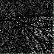
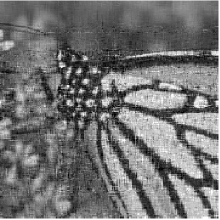
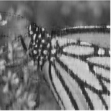
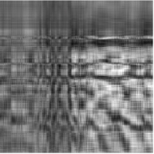
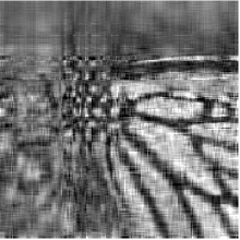
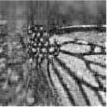
Figure 3: Top row (from left to right): observed Butterfly image with missing pixels ($\rho=0.3$), images recovered by BMC-GP-GAMP-I, BMC-GP-GAMP-II, and BMC-GP-GAMP-III, respectively. Bottom row (from left to right): images recovered by VSBL, LMaFit, BiGAMP-MC, and ALM-MC, respectively.

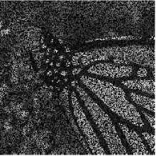
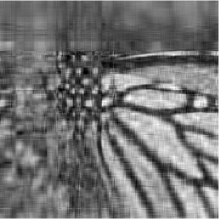
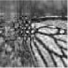
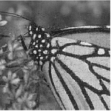
Figure 4: Top row (from left to right): observed Butterfly image with missing pixels ($\rho=0.5$), images recovered by BMC-GP-GAMP-I, BMC-GP-GAMP-II, and BMC-GP-GAMP-III, respectively. Bottom row (from left to right): images recovered by VSBL, LMaFit, BiGAMP-MC, and ALM-MC, respectively.

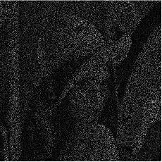
Figure 5: Top row (from left to right): observed Lena image with missing pixels ($\rho=0.2$), images recovered by BMC-GP-GAMP-I, BMC-GP-GAMP-II, and BMC-GP-GAMP-III, respectively. Bottom row (from left to right): images recovered by VSBL, LMaFit, BiGAMP-MC, and ALM-MC, respectively.

Figure 6: Top row (from left to right): observed Lena image with missing pixels ($\rho=0.3$), images recovered by BMC-GP-GAMP-I, BMC-GP-GAMP-II, and BMC-GP-GAMP-III, respectively. Bottom row (from left to right): images recovered by VSBL, LMaFit, BiGAMP-MC, and ALM-MC, respectively.

VI Conclusions

The problem of low-rank matrix completion was studied in this paper. A hierarchical Gaussian prior model was proposed to promote the low-rank structure of the underlying matrix, in which columns of the low-rank matrix are assumed to be mutually independent and follow a common Gaussian distribution with zero mean and a precision matrix. The precision matrix is treated as a random parameter, with a Wishart distribution specified as a hyperprior over it. Based on this hierarchical prior model, we developed a variational Bayesian method for matrix completion. To avoid cumbersome matrix inverse operations, the GAMP technique was used and embedded in the variational Bayesian inference, which resulted in an efficient VB-GAMP algorithm. Empirical results on synthetic and real datasets show that our proposed method offers competitive performance for matrix completion, and meanwhile achieves a significant reduction in computational complexity.

Appendix A Detailed Derivation of (7)

We provide a detailed derivation of (7). We have

$$p(\boldsymbol{X})= \int\prod\limits_{i=1}^{N}p(\boldsymbol{x}_{i}|\boldsymbol{\Sigma})p(\boldsymbol{\Sigma})d\boldsymbol{\Sigma}$$

$$\propto \int\left({\frac{|\boldsymbol{\Sigma}|}{(2\pi)^{M}}}\right)^{\frac{N}{2}}\exp(-\frac{1}{2}\text{tr}(\boldsymbol{X}^{T}\boldsymbol{\Sigma}\boldsymbol{X}))$$

$$\quad\times|\boldsymbol{\Sigma}|^{\frac{\nu-M-1}{2}}\exp(-\frac{1}{2}\text{tr}(\boldsymbol{W}^{-1}\boldsymbol{\Sigma}))d\boldsymbol{\Sigma}$$

$$\propto 2^{\frac{\nu M}{2}}\pi^{-\frac{MN}{2}}\Gamma_{M}\left(\frac{\nu+N}{2}\right)|\boldsymbol{W}^{-1}+\boldsymbol{X}\boldsymbol{X}^{T}|^{-\frac{\nu+N}{2}}$$

$$\times\int\frac{|\boldsymbol{\Sigma}|^{\frac{\nu+N-M-1}{2}}\exp(-\frac{1}{2}\text{Tr}((\boldsymbol{W}^{-1}+\boldsymbol{X}\boldsymbol{X}^{T})\boldsymbol{\Sigma}))}{2^{\frac{(\nu+N)M}{2}}|(\boldsymbol{W}^{-1}+\boldsymbol{X}\boldsymbol{X}^{T})^{-1}|^{\frac{\nu+N}{2}}\Gamma_{M}(\frac{\nu+N}{2})}d\boldsymbol{\Sigma}$$ (58)

where

$$\Gamma_{M}\left(x\right)=\pi^{\frac{M(M-1)}{4}}\prod_{j=1}^{M}\Gamma\left(x+\frac{1-j}{2}\right)$$ (59)

Note that the term in the integral of (58) is a standard Wishart distribution with $\nu+N$ degrees of freedom and variance matrix $(\boldsymbol{W}+\boldsymbol{X}\boldsymbol{X}^{T})^{-1}$. Thus we arrive at

$$p(\boldsymbol{X})\propto 2^{\frac{\nu M}{2}}\pi^{-\frac{MN}{2}}\Gamma_{M}\left(\frac{\nu+N}{2}\right)|\boldsymbol{W}^{-1}+\boldsymbol{X}\boldsymbol{X}^{T}|^{-\frac{\nu+N}{2}}$$

$$\propto |\boldsymbol{W}^{-1}+\boldsymbol{X}\boldsymbol{X}^{T}|^{-\frac{\nu+N}{2}}$$ (60)

Appendix B Proof of Lemma 1

Since we have $|\boldsymbol{X}\boldsymbol{X}^{T}+\boldsymbol{W}^{-1}|=|\boldsymbol{W}^{-1}||\boldsymbol{W}\boldsymbol{X}\boldsymbol{X}^{T}+\boldsymbol{I}|$, we only need to prove

$$|\boldsymbol{W}\boldsymbol{X}\boldsymbol{X}^{T}+\boldsymbol{I}|=|\boldsymbol{X}^{T}\boldsymbol{W}\boldsymbol{X}+\boldsymbol{I}|$$ (61)

Recalling the determinant of block matrices, we have

$$|\boldsymbol{W}\boldsymbol{X}\boldsymbol{X}^{T}+\boldsymbol{I}|=\begin{vmatrix}\boldsymbol{I}&\boldsymbol{X}^{T}\\ \boldsymbol{0}&\boldsymbol{W}\boldsymbol{X}\boldsymbol{X}^{T}+\boldsymbol{I}\end{vmatrix}$$ (62)

and

$$|\boldsymbol{I}|=\begin{vmatrix}\boldsymbol{I}&\boldsymbol{0}\\ -\boldsymbol{W}\boldsymbol{X}&\boldsymbol{I}\end{vmatrix}=\begin{vmatrix}\boldsymbol{I}&-\boldsymbol{X}^{T}\\ \boldsymbol{0}&\boldsymbol{I}\end{vmatrix}$$ (63)

which yields

$$|\boldsymbol{W}\boldsymbol{X}\boldsymbol{X}^{T}+\boldsymbol{I}|$$

$$= \begin{vmatrix}\boldsymbol{I}&\boldsymbol{X}^{T}\\ \boldsymbol{0}&\boldsymbol{W}\boldsymbol{X}\boldsymbol{X}^{T}+\boldsymbol{I}\end{vmatrix}$$

$$= \begin{vmatrix}\begin{bmatrix}\boldsymbol{I}&-\boldsymbol{X}^{T}\\ \boldsymbol{0}&\boldsymbol{I}\end{bmatrix}\begin{bmatrix}\boldsymbol{I}&\boldsymbol{0}\\ -\boldsymbol{W}\boldsymbol{X}&\boldsymbol{I}\end{bmatrix}\begin{bmatrix}\boldsymbol{I}&\boldsymbol{X}^{T}\\ \boldsymbol{0}&\boldsymbol{W}\boldsymbol{X}\boldsymbol{X}^{T}+\boldsymbol{I}\end{bmatrix}\end{vmatrix}$$

$$= \begin{vmatrix}\boldsymbol{X}^{T}\boldsymbol{W}\boldsymbol{X}+\boldsymbol{I}&\boldsymbol{0}\\ -\boldsymbol{W}\boldsymbol{X}&\boldsymbol{I}\end{vmatrix}$$

$$= |\boldsymbol{X}^{T}\boldsymbol{W}\boldsymbol{X}+\boldsymbol{I}|$$ (64)

Thus we have

$$\log|\boldsymbol{X}\boldsymbol{X}^{T}+\boldsymbol{W}^{-1}|=\log|\boldsymbol{W}^{-1}|+\log|\boldsymbol{I}+\boldsymbol{X}^{T}\boldsymbol{W}\boldsymbol{X}|$$ (65)

This completes the proof.

References

• [1] A. Karatzoglou, X. Amatriain, L. Baltrunas, and N. Oliver, “Multiverse recommendation: n-dimensional tensor factorization for context-aware collaborative filtering,” in Proceedings of the fourth ACM conference on Recommender systems, Barcelona, Spain, September 2010, pp. 79–86.
• [2] L. Xiong, X. Chen, T.-K. Huang, J. Schneider, and J. G. Carbonell, “Temporal collaborative filtering with Bayesian probabilistic tensor factorization,” in Proceedings of the 2010 SIAM International Conference on Data Mining, vol. 10, 2010, pp. 211–222.
• [3] G. Adomavicius and A. Tuzhilin, “Context-aware recommender systems,” in Recommender systems handbook.   Springer, 2011, pp. 217–253.
• [4] B. Jiang, S. Ma, J. Causey, L. Qiao, M. P. Hardin, I. Bitts, D. Johnson, S. Zhang, and X. Huang, “Sparrec: An effective matrix completion framework of missing data imputation for GWAS,” Scientific reports, vol. 6, 2016.
• [5] E. C. Chi, H. Zhou, G. K. Chen, D. O. D. Vecchyo, and K. Lange, “Genotype imputation via matrix completion,” Genome research, vol. 23, no. 3, pp. 509–518, 2013.
• [6] R. Cabral, F. D. la Torre, J. P. Costeira, and A. Bernardino, “Matrix completion for weakly-supervised multi-label image classification,” IEEE transactions on pattern analysis and machine intelligence, vol. 37, no. 1, pp. 121–135, 2015.
• [7] Y. Luo, T. Liu, D. Tao, and C. Xu, “Multiview matrix completion for multilabel image classification,” IEEE Transactions on Image Processing, vol. 24, no. 8, pp. 2355–2368, 2015.
• [8] W. Ye, L. Chen, G. Yang, H. Dai, and F. Xiao, “Anomaly-tolerant traffic matrix estimation via prior information guided matrix completion,” IEEE Access, vol. 5, pp. 3172–3182, 2017.
• [9] K. He and J. Sun, “Image completion approaches using the statistics of similar patches,” IEEE transactions on pattern analysis and machine intelligence, vol. 36, no. 12, pp. 2423–2435, 2014.
• [10] E. J. Candès and B. Recht, “Exact matrix completion via convex optimization,” Foundations of Computational mathematics, vol. 9, no. 6, p. 717, 2009.
• [11] B. Recht, M. Fazel, and P. A. Parrilo, “Guaranteed minimum-rank solutions of linear matrix equations via nuclear norm minimization,” SIAM review, vol. 52, no. 3, pp. 471–501, 2010.
• [12] M. Fazel, E. J. Candès, B. Recht, and P. A. Parrilo, “Compressed sensing and robust recovery of low rank matrices,” in 2008 42nd Asilomar Conference on Signals, Systems and Computers.   IEEE, 2008, pp. 1043–1047.
• [13] E. J. Candès and Yaniv, “Tight oracle inequalities for low-rank matrix recovery from a minimal number of noisy random measurements,” IEEE Transactions on Information Theory, vol. 57, no. 4, pp. 2342–2359, 2011.
• [14] J.-F. Cai, E. J. Candès, and Z. Shen, “A singular value thresholding algorithm for matrix completion,” SIAM Journal on Optimization, vol. 20, no. 4, pp. 1956–1982, 2010.
• [15] Z. Lin, M. Chen, and Y. Ma, “The augmented lagrange multiplier method for exact recovery of corrupted low-rank matrices,” arXiv preprint arXiv:1009.5055, 2010.
• [16] K. Mohan and M. Fazel, “Iterative reweighted least squares for matrix rank minimization,” in 2010 48th Annual Allerton Conference on Communication, Control, and Computing (Allerton).   IEEE, 2010, pp. 653–661.
• [17] D. Wipf, “Non-convex rank minimization via an empirical bayesian approach,” arXiv preprint arXiv:1408.2054, 2014.
• [18] Z. Kang, C. Kang, J. Cheng, and Q. Cheng, “Logdet rank minimization with application to subspace clustering,” Computational intelligence and neuroscience, vol. 2015, p. 68, 2015.
• [19] Z. Yang and L. Xie, “Enhancing sparsity and resolution via reweighted atomic norm minimization,” IEEE Transactions on Signal Processing, vol. 64, no. 4, pp. 995–1006, 2016.
• [20] S. D. Babacan, M. Luessi, R. Molina, and A. K. Katsaggelos, “Sparse Bayesian methods for low-rank matrix estimation,” IEEE Transactions on Signal Processing, vol. 60, no. 8, pp. 3964–3977, 2012.
• [21] M. Zhou, C. Wang, M. Chen, J. Paisley, D. Dunson, and L. Carin, “Nonparametric Bayesian matrix completion,” in 2010 IEEE Sensor Array and Multichannel Signal Processing Workshop (SAM).   IEEE, 2010, pp. 213–216.
• [22] J. T. Parker, P. Schniter, and V. Cevher, “Bilinear generalized approximate message passing – Part I: Derivation,” IEEE Transactions on Signal Processing, vol. 62, no. 22, pp. 5839–5853, 2014.
• [23] ——, “Bilinear generalized approximate message passing – Part II: Applications,” IEEE Transactions on Signal Processing, vol. 62, no. 22, pp. 5854–5867, 2014.
• [24] B. Xin, Y. Wang, W. Gao, and D. Wipf, “Exploring algorithmic limits of matrix rank minimization under affine constraints,” IEEE Transactions on Signal Processing, vol. 64, no. 19, pp. 4960–4974, 2016.
• [25] Z. Zhang and B. D. Rao, “Sparse signal recovery with temporally correlated source vectors using sparse Bayesian learning,” IEEE Journal of Selected Topics in Signal Processing, vol. 5, no. 5, pp. 912–926, Sep. 2011.
• [26] P. J. Everson and C. N. Morris, “Inference for multivariate normal hierarchical models,” Journal of the Royal Statistical Society: Series B (Statistical Methodology), vol. 62, pp. 399–412, Mar. 2000.
• [27] C. M. Bishop, Pattern recognition and machine learning.   Springer, 2007.
• [28] E. Candés, M. Wakin, and S. Boyd, “Enhancing sparsity by reweighted $l_{1}$ minimization,” Journal of Fourier Analysis and Applications, vol. 14, pp. 877–905, Dec. 2008.
• [29] Y. Shen, J. Fang, and H. Li, “Exact reconstruction analysis of log-sum minimization for compressed sensing,” IEEE Signal Processing Letters, vol. 20, pp. 1223–1226, Dec. 2013.
• [30] X. Fu, K. Huang, W.-K. Ma, N. D. Sidiropoulos, and R. Bro, “Joint tensor factorization and outlying slab suppression with applications,” IEEE Transactions on Signal Processing, vol. 63, no. 23, pp. 6315–6328, 2015.
• [31] Z. Chen, R. Molina, and A. K. Katsaggelos, “Robust recovery of temporally smooth signals from under-determined multiple measurements,” IEEE Transactions on Signal Processing, vol. 63, no. 7, pp. 1779–1791, 2015.
• [32] D. I. Shuman, S. K. Narang, P. Frossard, A. Ortega, and P. Vandergheynst, “The emerging field of signal processing on graphs: Extending high-dimensional data analysis to networks and other irregular domains,” IEEE Signal Processing Magazine, pp. 83–98, May 2013.
• [33] S. Kullback and R. A. Leibler, “On information and sufficiency,” The annals of mathematical statistics, pp. 79–86, 1951.
• [34] D. G. Tzikas, A. C. Likas, and N. P. Galatsanos, “The variational approximation for Bayesian inference,” IEEE Signal Processing Magazine, pp. 131–146, Nov. 2008.
• [35] S. Rangan, “Generalized approximate message passing for estimation with random linear mixing,” in Proc. IEEE Int. Symp. Inf. Theory (ISIT), Saint Petersburg, Russia, Aug. 2011.
• [36] D. L. Donoho, A. Maleki, and A. Montanari, “Message passing algorithms for compressed sensing: I. motivation and construction,” in Proc. Inf. Theory Workshop, Cairo, Egypt, Jan. 2010.
• [37] Z. Wen, W. Yin, and Y. Zhang, “Solving a low-rank factorization model for matrix completion by a nonlinear successive over-relaxation algorithm,” Mathematical Programming Computation, vol. 4, no. 4, pp. 333–361, Dec. 2012.