Hierarchical space-time modeling of asymptotically independent exceedances with an application to precipitation data

Abstract

The statistical modeling of space-time extremes in environmental applications is key to understanding complex dependence structures in original event data and to generating realistic scenarios for impact models. In this context of high-dimensional data, we propose a novel hierarchical model for high threshold exceedances defined over continuous space and time by embedding a space-time Gamma process convolution for the rate of an exponential variable, leading to asymptotic independence in space and time. Its physically motivated anisotropic dependence structure is based on geometric objects moving through space-time according to a velocity vector. We demonstrate that inference based on weighted pairwise likelihood is fast and accurate. The usefulness of our model is illustrated by an application to hourly precipitation data from a study region in Southern France, where it clearly improves on an alternative censored Gaussian space-time random field model. While classical limit models based on threshold-stability fail to appropriately capture relatively fast joint tail decay rates between asymptotic dependence and classical independence, strong empirical evidence from our application and other recent case studies motivates the use of more realistic asymptotic independence models such as ours.

Keywords: Asymptotic independence, space-time extremes, gamma random fields, space-time convolution, composite likelihood, hourly precipitation.

1 Introduction

The French Mediterranean area is subject to heavy rainfall events occurring mainly in the fall season. Intense precipitation often leads to flash floods, which can be defined as a sudden strong rise of the water level. Flash floods often cause fatalities and important material damage. In the literature, such intense rainfalls are often called flood-risk rainfall (Carreau and Bouvier, 2016); characterizing their spatio-temporal dependencies is key to understanding these processes. In this paper, we consider a large data set of hourly precipitation measurements from a study region in Southern France. We tackle the challenge of proposing a physically interpretable statistical space-time model for high threshold exceedances, which aims to capture the complex dependence and time dynamics of the data process.

Fueled by important environmental applications during the last decade, the statistical modeling of spatial extremes has undergone a fast evolution. A shift from maxima-based modeling to approaches using threshold exceedances can be observed over recent years, whose reasons lie in the capability of thresholding techniques to exploit more information from the data and to explicitly model the original event data. A first overview of approaches to modeling maxima is due to Davison et al. (2012). A number of hierarchical models based on latent Gaussian processes (Casson and Coles, 1999; Gaetan and Grigoletto, 2007; Cooley et al., 2007; Sang and Gelfand, 2009) have been proposed, but they may be criticized for relying on the rather rigid Gaussian dependence with very weak dependence in the tail, while the lack of closed-form marginal distributions makes interpretation difficult and frequentist inference cumbersome. Max-stable random fields (Smith, 1990; Schlather, 2002; Kabluchko et al., 2009; Davison and Gholamrezaee, 2012; Reich and Shaby, 2012; Opitz, 2013) are the natural limit models for maxima data and have spawned a very rich literature, from which the model of Reich and Shaby (2012) stands out for its hierarchical construction simplifying high-dimensional multivariate calculations and Bayesian inference. Generalized Pareto processes (Ferreira and de Haan, 2014; Opitz et al., 2015; Thibaud and Opitz, 2015) are the equivalent limit models for threshold exceedances. However, the asymptotic dependence stability in these limiting processes for maxima and threshold exceedances has a tendency to be overly restrictive when asymptotic dependence strength decreases at high levels and may vanish ultimately in the case of asymptotic independence. The results from the empirical spatio-temporal exploration of our French rainfall data in Section 6.2 are strongly in favor of asymptotic independence, which appears to be characteristic for many environmental data sets (Davison et al., 2013; Thibaud et al., 2013; Tawn et al., 2018) and may arise from physical laws such as the conservation of mass. This has motivated the development of more flexible dependence models, such as max-mixtures of max-stable and asymptotically independent processes (Wadsworth and Tawn, 2012; Bacro et al., 2016) or max-infinitely divisible constructions (Huser et al., 2018) for maxima data, or Gaussian scale mixture processes (Opitz, 2016; Huser et al., 2017) for threshold exceedances, capable to accommodate asymptotic dependence, asymptotic independence and Gaussian dependence with a smooth transition. Other flexible spatial constructions involve marginally transformed Gaussian processes (Huser and Wadsworth, 2018). Such threshold models can be viewed as part of the wider class of copula models (see Bortot et al., 2000; Davison et al., 2013, for other examples) typically combining univariate limit distributions with dependence structures that should ideally be flexible and relatively easy to handle in practice.

Statistical inference is then often carried out assuming temporal independence in measurements typically observed at spatial sites at regularly spaced time intervals. However, developing flexible space-time modeling for extremes is crucial for characterizing the temporal persistence of extreme events spanning several time steps; such models are important for short-term prediction in applications such as the forecasting of wind power and atmospheric pollution, and for extreme event scenario generators providing inputs to impact models, for instance in hydrology and agriculture. Early spatio-temporal models for rainfall were proposed in the 1980s (Rodriguez-Iturbe et al., 1987; Cox and Isham, 1988, and the references therein) and exploit the idea that storm events give rise to a cluster of rain cells, which are represented as cylinders in space-time. Currently, only few statistical space-time models for extremes are available. Davis and Mikosch (2008) consider extremal properties of heavy-tailed moving average processes where coefficients and the white-noise process depend on space and time, but their work was not focused on practical modeling. Sang and Gelfand (2009) propose a hierarchical procedure for maxima data but limited to latent Gauss–Markov random fields. Davis et al. (2013a, b) extend the widely used class of Brown–Resnick max-stable processes to the space-time framework and propose pairwise likelihood inference. Spatial max-stable processes with random set elements have been proposed by Schlather (2002); Davison and Gholamrezaee (2012), and Huser and Davison (2014) have fitted a space-time version to threshold exceedances of hourly rainfall data through pairwise censored likelihood. Huser and Davison (2014) model storms as discs of random radius moving at a random velocity for a random duration, leading to randomly centered space-time cylinders; our models developed in the following rely on similar geometric representations. A Bayesian approach based on spatial skew-$t$ random fields with a random set element and temporal autoregression was proposed by Morris et al. (2017). The aforementioned space-time models may capture asymptotic dependence or exact independence at small distances but are unsuitable for dealing with residual dependence in asymptotic independence. In this paper, we propose a novel approach to space-time modeling of asymptotically independent data to avoid the tendency of max-stable-like models to potentially strongly overestimate joint extreme risks. In a similar context, Nieto-Barajas and Huerta (2017) have recently proposed a spatio-temporal Pareto model for heavy-tailed data on spatial lattices, generalizing the temporal latent process model of Bortot and Gaetan (2014) to space-time.

Our model provides a hierarchical formulation for modeling spatio-temporal exceedances over high thresholds. It is defined over a continuous space-time domain and allows for a physical interpretation of extreme events spreading over space and time. Strong motivation also comes from Bortot and Gaetan (2014) by developing a generalization of their latent temporal process. Alternatively, our latent process could be viewed as a space-time version of the temporal trawl processes introduced by Barndorff-Nielsen et al. (2014) and exploited for extreme values by Noven et al. (2015), with spatial extensions recently proposed by Opitz (2017). Our approach is based on representing a generalized Pareto distribution as a Gamma mixture of an exponential distribution, enabling us to keep easily tractable marginal distributions which remain coherent with univariate extreme value theory. We use a kernel convolution of a space-time Gamma random process (Wolpert and Ickstadt, 1998a) based on influence zones defined as cylinders with an ellipsoidal basis to generate anisotropic spatio-temporal dependence in exceedances. We then develop statistical inference based on pairwise likelihood.

The paper is structured as follows. Our hierarchical model with a detailed description of its two stages and marginal transformations is developed in Section 2. Space-time Gamma random fields are presented in Section 7 where we also propose the construction and formulas for the space-time objects used for kernel convolution. Section 3 characterizes tail dependence behavior in our new model yielding asymptotic independence in space and time. Statistical inference of model parameters is addressed in Section 4 based on a pairwise log-likelihood for the observed censored excesses. We show good estimation performance through a simulation study presented in Section 5 involving two scenarios of different complexity. In Section 6, we focus on the dataset and explore in detail how our fitted space-time model captures spatio-temporal extremal dependence in hourly precipitation. Since a natural choice of a reference model for asymptotically independent data is to use threshold-censored space-time Gaussian processes, we show the good relative performance of our model by comparing it to such alternatives. A discussion of our modeling approach with some potential future extensions closes the paper in Section 7.

2 A hierarchical model for spatio-temporal exceedances

When dealing with exceedances of a random variable $X$ above a high threshold $u$, univariate extreme value theory suggests using the limit distribution of Generalized Pareto (GP) type. The GP cumulative distribution function (cdf) is defined for any $y>0$ by

$$GP(y;\sigma,\xi)=1-\left(1+\xi\frac{y}{\sigma}\right)_{+}^{-(1/\xi)},$$ (1)

where $(a)_{+}=\max(0,a)$, $\xi$ is a shape parameter and $\sigma$ a positive scale parameter. The sign of $\xi$ characterizes the maximum domain of attraction of the distribution of $X$: $\xi>0$ corresponds to the Fréchet domain of attraction while $\xi=0$ and $\xi<0$ correspond to the Gumbel and Weibull ones, respectively.

When $\xi>0$, the GP distribution can be expressed as a Gamma mixture for the rate of the exponential distribution (Reiss and Thomas, 2007, p.157), i.e.

$$V|\Lambda\sim{\mbox{Exp}}(\Lambda),\quad\Lambda\sim{\mbox{Gamma}}(1/\xi,\sigma/\xi)\quad\Rightarrow\quad V\sim GP(\,\cdot\,;\sigma,\xi),$$ (2)

where $\mathrm{Exp}(b)$ refers to the Exponential distribution with rate $b>0$ and $\mathrm{Gamma}(a,b)$ to the Gamma distribution with shape $a>0$ and rate $b>0$. Based on this hierarchical structure, we will here develop a stationary space-time construction for modeling exceedances over a high threshold, which possesses marginal GP distributions for the strictly positive excess above the threshold.

2.1 First stage: generic hierarchical space-time structure

We consider a stationary space-time random field $Z=\{Z(x),x\in\mathcal{X}\}$ with $x=(s,t)$ and $\mathcal{X}=\mathbb{R}^{2}\times\mathbb{R}^{+}$, such that $s$ indicates spatial location and $t$ time. Without loss of generality, we assume that the margins $Z(x)$ belong to the Fréchet domain of attraction with positive shape parameter $\xi$. To infer the tail behavior of $\{Z(x)\}$, we focus on values exceeding a fixed high threshold $u$, and we consider the exceedances over $u$,

$$Y(x)=(Z(x)-u)\cdot\mathbf{1}_{(u,\infty)}(Z(x)).$$ (3)

Standard results from extreme value theory (de Haan and Ferreira, 2006) establish the $GP$ distribution with $\xi>0$ in (1) as the limit of suitably renormalized positive threshold exceedances in (3), such that it represents a natural model for the values $Y(x)>0$. Following Bortot and Gaetan (2014), we use the representation of the $GP$ distribution as a Gamma mixture of an exponential distribution to formulate a two-stage model that induces spatio-temporal dependence arising in both the exceedance indicators $\mathbf{1}_{(u,\infty)}(Z(x))$ and the positive excesses $Z(x)-u>0$ by integrating space-time dependence in a latent Gamma component. A key feature of our model is that it naturally links exceedance probability to the size of the excess and therefore provides a joint space-time structure of the zero part and the positive part in the zero-inflated distribution of $Y(x)$.

In the first stage, we condition on a latent space-time random field $\{\Lambda(x)\}$ with marginal distributions $\Lambda(x)\sim\textrm{Gamma}(\alpha,\beta)$ and assume that

$$Y(x)\mid\left[\Lambda(x),Y(x)>0\right] \sim{\mbox{Exp}}\left(\Lambda(x)\right),$$ (4a)

$$\Pr(Y(x)>0\mid\Lambda(x)) =e^{-\kappa\Lambda(x)},$$ (4b)

where $\kappa>0$ is a parameter controlling the rate of upcrossings of the threshold. The resulting marginal distribution of $Y(x)$ conditionally on $Z(x)>u$ corresponds to the GP distribution, and the unconditional marginal cdf of $Y(x)$ is

$$F(y;\sigma,\xi)=\left\{\begin{array}[]{lc}p&\textrm{for }y=0,\\ p+(1-p)GP(y;\xi,\sigma)&\textrm{for }y>0,\end{array}\right.$$ (5)

with shape parameter $\xi=1/\alpha$, scale parameter $\sigma=(\kappa+\beta)/\alpha$, and with $1-p$ the probability of an exceedance over $u$, i.e. $\Pr(Z(x)>u)=\Pr(Y(x)>0)=1-p$. The probability of exceeding $u$,

$$\Pr(Z(x)>u)=\mathrm{E}\left(\Pr(Y(x)>0|\Lambda(x))\right)=\mathrm{E}\left(e^{-\kappa\Lambda(x)}\right)=\left(\frac{\beta}{\kappa+\beta}\right)^{\alpha}$$ (6)

depends on $\kappa$ and corresponds to the Laplace transform of $\Lambda(x)$ evaluated at $\kappa$. The constraint $\xi>0$ is not restrictive for dealing with precipitation in the French Mediterranean area, which is known to be heavy-tailed. For general modeling purposes, we can relax this assumption by following Bortot and Gaetan (2016): we consider a marginal transformation within the class of GP distributions for threshold exceedances, for which we suppose that $\alpha=1$ and $\beta=1$ for identifiability. By transforming $Y(x)$ through the probability integral transform

$$g(y)=GP^{-1}(GP(y;1,1+\kappa);\sigma^{*},\xi^{*})=(\sigma^{*}/{\xi^{*}})\left\{\left(1+\frac{y}{\kappa+1}\right)^{\xi^{*}}-1\right\}$$ (7)

with parameters $\xi^{*}\in\mathbb{R}$ and $\sigma^{*}>0$ to be estimated, we get a marginally transformed random field $Y^{*}(x)=g(Y(x))$ which satisfies $Y^{*}(x)\sim GP(\,\cdot\,;\xi^{*},\sigma^{*})$, conditionally on $Y^{*}(x)>0$. Notice that it is straightforward to develop extensions with nonstationary marginal excess distributions by injecting response surfaces $\sigma^{\star}(x)$ and $\xi^{\star}(x)$ into (7). Moreover, nonstationarity could be introduced into the latent Gamma model (4) in different ways. If $\kappa=\kappa(x)$ depends on $x$ or other covariate information, exceedance probabilites become nonstationary. If Gamma parameters $\alpha=\alpha(x)$ and $\beta=\beta(x)$ depend on covariates, then the GP margins in $Y(x)$ become nonstationary. Finally, one could combine the two previous nonstationary extensions.

2.2 Second stage: space-time dependence with Gamma random fields

Spatio-temporal dependence is introduced by means of a space-time stationary random field $\{\Lambda(x),x\in\mathcal{X}\}$ with $\mathrm{Gamma}(\alpha,\beta)$ marginal distributions. In principle, we could use an arbitrarily wide range of models with any kind of space-time dependence structure, for instance by marginally transforming a space-time Gaussian random field using the copula idea (Joe, 1997). However, we here aim to propose a construction where Gamma marginal distributions arise naturally without applying rather artificial marginal transformations. Inspired by the Gamma process convolutions of Wolpert and Ickstadt (1998a), we develop a space-time Gamma convolution process with Gamma marginal distributions. The kernel shape in our construction allows for a straightforward interpretation of the dependence structure, and it offers a physical interpretation of real phenomena such as mass and particle transport. Moreover, we obtain simple analytical formulas for the bivariate distributions, which facilitates statistical inference, interpretation and the characterization of joint tail properties.

We fix $\mathcal{X}=\mathbb{R}^{3}$ and consider $A\in\mathcal{B}_{b}(\mathcal{X})$, a subset of $\mathcal{X}$ belonging to the $\sigma-$field $\mathcal{B}_{b}(\mathcal{X})$ restricted to bounded sets of $\mathcal{X}$. A Gamma random field $\Gamma(dx)$ (Ferguson, 1973) is a non negative random measure defined on $\mathcal{X}$ characterized by a base measure $\alpha(dx)$ and a rate parameter $\beta$ such that

1. $\Gamma(A):=\int_{A}\Gamma(dx)\sim\textrm{Gamma}(\alpha(A),\beta)$, with $\alpha(A):=\int_{A}\alpha(dx)$;

2. for any $A_{1},A_{2}\in\mathcal{B}_{b}(\mathcal{X})$ such that $A_{1}\cap A_{2}=\emptyset$, $\Gamma(A_{1})$ and $\Gamma(A_{2})$ are independent random variables.

The calculation of important formulas in this paper requires the Laplace exponent of the random measure given as

$$\mathcal{L}(\phi):=-\log\mathrm{E}\left(\exp\left\{-\int\phi(x)\Gamma(dx)\right\}\right)=\int_{\mathcal{X}}\log\left\{1+\frac{\phi(x)}{\beta}\right\}\alpha(dx)$$

where $\phi$ is any positive measurable function; in our case, it will represent the kernel function (see the Appendix section 8). We propose to model $\{\Lambda(x),x\in\mathcal{X}\}$ as a convolution using a 3D indicator kernel $K(x,x^{\prime})$ with an indicator set of finite volume used to convolve the Gamma random field $\Gamma(dx)$ (Wolpert and Ickstadt, 1998a), i.e., $\Lambda(x)=\int K(x,x^{\prime})\Gamma(dx^{\prime})$. The shape of the kernel can be very general (although non indicator kernels usually do not lead to Gamma marginal distributions), and particular choices may lead to nonstationary random fields, or to stationary random fields with given dependence properties such as full symmetry, separability or independence beyond some spatial distance or temporal lag. In order to limit model complexity and computational burden to a reasonable amount, we use the indicator kernel $K(x,x^{\prime})=\mathbf{1}_{A}(x-x^{\prime})$, for $A\in\mathcal{B}_{b}(\mathcal{X})$, where $A$ is given as a slated elliptical cylinder, defining a $3$-dimensional set $A_{x}$ that moves through $\mathcal{X}$ according to some velocity vector. More precisely, let $E(s,\gamma_{1},\gamma_{2},\phi)$ be an ellipse centered at $s=(s_{1},s_{2})\in\mathbb{R}^{2}$ (see Figure 1-(a)), whose axes are rotated counterclockwise by the angle $\phi$ with respect to the coordinate axes, whose semi-axes’ lengths in the rotated coordinate system are $\gamma_{1}$ and $\gamma_{2}$, respectively. A physical interpretation is that the ellipse describes the spatial influence zone of a storm centered at $s$. For the temporal dynamics, we assume that the ellipses (storms) $E(s,\gamma_{1},\gamma_{2},\phi)$ move through space with a velocity $\omega=(\omega_{1},\omega_{2})\in\mathbb{R}^{2}$ for a duration $\delta>0$. The volume of the intersection of two slated elliptical cylinders (see Figure 1-(b)) is given by

$$V(s,t,s^{\prime},t^{\prime})=(\delta-|t-t^{\prime}|)_{+}\times\nu_{2}(E(s,\gamma_{1},\gamma_{2},\phi)\cap E(\tilde{s},,\gamma_{1},\gamma_{2},\phi))$$

where $\tilde{s}=(\tilde{s_{1}},\tilde{s_{2}})$ with $\tilde{s_{i}}=s_{i}^{\prime}-|t^{\prime}-t|\times\omega_{i}$, $i=1,2$, where $\nu_{d}(\cdot)$ is the Lebesgue measure on $\mathbb{R}^{d}$.

For two fixed locations, the strength of dependence in the random field $\Lambda(x)$ is an increasing monotone function of the intersection volume; other choices of $A$ are possible, provided that we are able to calculate efficiently the volume of the intersection. To efficiently calculate the ellipse intersection area, we use an approach for finding the overlap area between two ellipses, which does not rely on proxy curves; see Hughes and Chraibi (2012).

In the sequel, we consider the measure

$$\alpha(B)=\alpha\nu_{d}(B)/\nu_{d}(A),\quad B\in\mathcal{B}_{b}(\mathcal{X}).$$ (8)

It follows that $\Lambda(x)\sim\textrm{Gamma}(\alpha,\beta)$, as required for model (4). Exploiting the formulas of the Appendix section 8, the univariate Laplace transform of $\Lambda(x)$ is

$$LP_{x}^{(1)}(v):=\mathrm{E}\left(e^{-v\Lambda(x)}\right)=\left(\frac{\beta}{v+\beta}\right)^{\alpha},$$ (9)

and the bivariate Laplace transform of $\Lambda(x)$ and $\Lambda({x^{\prime}})$ is

$$LP_{x,x^{\prime}}^{(2)}(v_{1},v_{2}) := \mathrm{E}\left(e^{-v_{1}\Lambda(x)-v_{2}\Lambda({x^{\prime}})}\right)$$ (10)

$$= \left(\frac{\beta}{v_{1}+\beta}\right)^{\alpha(A_{x}\backslash A_{x^{\prime}})}\left(\frac{\beta}{v_{1}+v_{2}+\beta}\right)^{\alpha(A_{x}\cap A_{x^{\prime}})}\left(\frac{\beta}{v_{2}+\beta}\right)^{\alpha(A_{x^{\prime}}\backslash A_{x})}.$$

This model for $\Lambda(x)$ is stationary, but nonstationarity in Gamma marginal distributions and/or dependence can be generated by using nonstationary indicator sets $A_{x}$ whose size and shape depends on $x$. More general sets $A_{x}$ with finite Lebesgue volume $\nu_{3}(A_{x})$ could be used for constructing $\Lambda(x)=\Gamma(A_{x})$. In all cases, the intersecting volume $\nu_{3}(A_{x_{1}}\cap A_{x_{2}})$ tends to zero if $\|x_{2}-x_{1}\|\rightarrow\infty$, which establishes the property of $\alpha$-mixing over space and time for the processes $\Lambda(x)$ and $Y(x)$. This property is paramount to ensure consistency and asymptotic normality in the pairwise likelihood estimation that we consider in the following (see Huser and Davison (2014)).

3 Joint tail behavior of the hierarchical process

Extremal dependence in a bivariate random vector $(Z_{1},Z_{2})$ can be explored based on the tail behavior of the conditional distribution $\Pr(Z_{1}>F_{1}^{\leftarrow}(q)|Z_{2}>F_{2}^{\leftarrow}(q))$ as $q$ tends to $1$, where $F_{i}^{\leftarrow}$, $i=1,2$ denotes the generalized inverse distribution functions of $Z_{i}$ (Sibuya, 1960; Coles et al., 1999). The random vector $(Z_{1},Z_{2})$ is said to be asymptotically dependent if a positive limit $\chi$, referred to as the tail correlation coefficient, arises:

$$\chi(q):=\frac{\Pr(Z_{1}>F_{1}^{\leftarrow}(q),Z_{2}>F_{2}^{\leftarrow}(q))}{\Pr(Z_{2}>F_{2}^{\leftarrow}(q))}\rightarrow\chi>0,\qquad q\rightarrow 1^{-}.$$

The case $\chi=0$ characterizes asymptotic independence.

To obtain a finer characterization of the joint tail decay rate under asymptotic independence, faster than the marginal tail decay rate, Coles et al. (1999) have introduced the $\overline{\chi}$ index defined through the limit relation

$$\bar{\chi}(q):=\frac{2\log\Pr(Z_{2}>F_{2}^{\leftarrow}(q))}{\log{\Pr}(Z_{1}>F_{1}^{\leftarrow}(q),Z_{2}>F_{2}^{\leftarrow}(q))}-1\rightarrow\bar{\chi}\in(-1,1],\qquad q\rightarrow 1^{-}.$$

Larger values of $|\bar{\chi}|$ correspond to stronger dependence. We now show that $\{Z(x),x\in\mathcal{X}\}$ is an asymptotic independent process, i.e., for all pairs $(x,x^{\prime})\in\mathcal{X}^{2}$ with $x\not=x^{\prime}$ the bivariate random vectors $(Z(x),Z(x^{\prime}))$ are asymptotically independent.

Owing to the stationarity of the process, it is easy to show that for any $(x,x^{\prime})\in\mathcal{X}^{2}$, $x\not=x^{\prime}$ and for values $v$ exceeding a threshold $u\geq 0$, we get

$$\Pr(Z(x)>v) = LP_{x}^{(1)}(v-u+\kappa)$$

$$= \left(1+\frac{v-u+\kappa}{\beta}\right)^{-\alpha(A_{x})}$$

and

$$\Pr(Z(x)>v,Z(x^{\prime})>v) = LP_{x,x^{\prime}}^{(2)}(v-u+\kappa,v-u+\kappa)$$

$$= \left(1+\frac{v-u+\kappa}{\beta}\right)^{-\alpha(A_{x}\backslash A_{x^{\prime}})}\left(1+\frac{2v-2u+2\kappa}{\beta}\right)^{-\alpha(A_{x}\cap A_{x^{\prime}})}$$

$$\times\left(1+\frac{v-u+\kappa}{\beta}\right)^{-\alpha(A_{x^{\prime}}\backslash A_{x})}.$$

To simplify notations, we set $c_{0}:=\alpha(A_{x})$, $c_{1}:=\alpha(A_{x}\backslash A_{x^{\prime}})$, $c_{2}:=\alpha(A_{x}\cap A_{x^{\prime}})$ , $c_{3}:=\alpha(A_{x^{\prime}}\backslash A_{x})$, such that $c_{1}=c_{3}=c_{0}-c_{2}\geq 0$ and $c_{1}+2c_{2}+c_{3}=2c_{0}$. For $c_{2}=0$ characterizing disjoint indicator sets $A_{x}$ and $A_{x^{\prime}}$, it is clear that $Z(x)$ and $Z(x^{\prime})$ are independent. Now, assume $u=0$ without loss of generality and $x\not=x^{\prime}$; then,

$$\chi_{x,x^{\prime}}(v) := \frac{\Pr(Z(x)>v,Z(x^{\prime})>v)}{\Pr(Z(x^{\prime})>v)}$$

$$= \left(1+\frac{2v+2\kappa}{\beta}\right)^{-c_{2}}\left(1+\frac{v+\kappa}{\beta}\right)^{-c_{1}-c_{3}+c_{0}}$$

$$= \left(1+\frac{2v+2\kappa}{\beta}\right)^{-c_{2}}\left(1+\frac{v+\kappa}{\beta}\right)^{2c_{2}-c_{0}}$$

$$\sim {2}^{-c_{2}}\left(\frac{v}{\beta}\right)^{c_{2}-c_{0}},\qquad\mbox{for large $v$}.$$

Since $c_{2}<c_{0}$, we obtain

$$\chi_{x,x^{\prime}}=0.$$

We conclude that $Z$ is an asymptotic independent process.

To characterize the faster joint tail decay, we calculate

$$\bar{\chi}_{xx^{\prime}}(v) := \frac{2\log{\rm Pr}(Z(x)>v)}{\log{\rm Pr}(Z(x)>v,Z(x^{\prime})>v)}-1$$

$$= \cfrac{-2c_{0}\log\left(1+(v+\kappa)/{\beta}\right)}{-c_{1}\log(1+(v+k)/{\beta})-c_{2}\log\left(1+2(v+k)/{\beta}\right)-c_{3}\log(1+(v+k)/{\beta})}-1$$

$$= \cfrac{2c_{0}}{c_{1}+c_{2}\cfrac{\log\left(1+2(v+k)/{\beta}\right)}{\log\left(1+(v+k)/\beta\right)}+c_{3}}-1.$$

Taking the limit for $v\rightarrow\infty$ yields

$$\bar{\chi}_{x,x^{\prime}}=\cfrac{2c_{0}}{c_{1}+c_{2}+c_{3}}-1=\cfrac{c_{2}}{2c_{0}-c_{2}},$$

which describes the ratio between the intersecting volume of $A_{x}$ and $A_{x^{\prime}}$ and the volume of the union of these two sets. The value of $\bar{\chi}$ confirms the asymptotic independence of the process $Z$. A larger intersecting volume between $A_{x}$ and $A_{x^{\prime}}$ corresponds to stronger dependence.

4 Composite likelihood inference

To infer the tail behavior of the observed data process $\{Z(x)\}$, without loss of generality assumed to have generalized Pareto marginal distributions with shape parameter $\alpha$, we focus on values exceeding a fixed high threshold $u$. We let $\theta$ denote the vector of unknown parameters. For simplicity, we assume that we have observed the excess values $Y(s_{i},t)$ for a factorial design of $S$ locations $s_{i}$, $i=1,\ldots,S$ and $T$ times $t=1,\ldots,T$.

To exploit the tractability of intersecting volumes of two kernel sets, we focus on pairwise likelihood for efficient inference in our high-dimensional space-time set-up. The pairwise (weighted) log-likelihood adds up the contributions $f(Y(s_{i},t),Y(s_{j},t+k);\theta)$ of the censored observations $Y(s_{i},t),Y(s_{j},t+k)$ and can be written

$$\mathrm{pl}(\theta)=\sum_{t=1}^{T}\mathrm{pl}_{t}(\theta)=\sum_{t=1}^{T}\sum_{k=0}^{\Delta_{T}}\sum_{i=1}^{S}\sum_{j=1}^{S}\{1-{1}_{\{i\geq j,\,k=0\}}\}\log f(Y(s_{i},t),Y(s_{j},t+k);\theta){w_{s_{i},s_{j}}}$$ (11)

where $w_{s_{i},s_{j}}$ is a weight defined on $[0,\infty)$ (Bevilacqua et al., 2012; Davis et al., 2013b; Huser and Davison, 2014). We opt for a cut-off weight with $w_{s_{i},s_{j}}=1$ if $||s_{i}-s_{j}||\leq\Delta_{S}$ and $0$ otherwise, which bypasses an explosion of the number of likelihood terms and shifts focus to relatively short-range distances where dependence matters most. This also avoids that the pairwise likelihood value (and therefore parameter estimation) is dominated by a large number of intermediate-range distances where dependence has already decayed to (almost) nil.

The contributions $f(Y(x),Y(x^{\prime});\theta)$ are given by

$$f(y_{1},y_{2};\theta)=\left\{\begin{array}[]{ll}\frac{\partial^{2}}{\partial v_{1}\partial v_{2}}LP^{(2)}_{x,x^{\prime}}(v_{1},v_{2})J(y_{1})J(y_{2})&y_{1}>0,y_{2}>0\\ \left(-\frac{\partial}{\partial v_{1}}LP^{(1)}(v_{1})+\frac{\partial}{\partial v_{1}}LP_{x,x^{\prime}}^{(2)}(v_{1},v_{2})\right)J(y_{1})&y_{1}>0,y_{2}=0\\ \left(-\frac{\partial}{\partial v_{2}}LP^{(1)}(v_{2})+\frac{\partial}{\partial v_{2}}LP_{x,x^{\prime}}^{(2)}(v_{1},v_{2})\right)J(y_{2})&y_{1}=0,y_{2}>0\\ 1-2LP^{(1)}(v_{1})+LP_{x,x^{\prime}}^{(2)}(v_{1},v_{2})&y_{1}=0,y_{2}=0\end{array}\right.$$

with $v_{i}=(\kappa+1)\left(1+\xi^{*}y_{i}/\sigma^{*}\right)^{1/\xi^{*}}-1$ and $J(y_{i})=\frac{\kappa+1}{\sigma^{*}}\left(1+\frac{\xi^{*}y_{i}}{\sigma^{*}}\right)^{1/\xi^{*}-1}$, $i=1,2$. We provide analytical expressions for $LP^{(1)}$ and $LP_{x,x^{\prime}}^{(2)}$ in the Appendix section 9.

Since the space-time random field $\{\Lambda(x)\}$ is temporally $\alpha$-mixing, the maximum pairwise likelihood estimator $\widehat{\theta}$ can be shown to be asymptotically normal for large $T$ under mild additional regularity conditions; see Theorem 1 of Huser and Davison (2014). The asymptotic variance is given by the inverse of the Godambe information matrix $\mathcal{G}(\theta)=\mathcal{H}(\theta)[\mathcal{J}(\theta)]^{-1}\mathcal{H}(\theta)$. Therefore, standard error evaluation requires consistent estimation of the matrices $\mathcal{H}(\theta)=\mathrm{E}(-\nabla^{2}\mathrm{pl}(\theta))$ and $\mathcal{J}(\theta)=\mathrm{Var}(\nabla\mathrm{pl}(\theta))$. We estimate $\mathcal{H}(\theta)$ with $\widehat{\mathcal{H}}=-\nabla^{2}\mathrm{pl}(\widehat{\theta})$ and $\mathcal{J}(\theta)$ through a subsampling technique (Carlstein, 1986), implemented as follows. We define $B$ overlapping blocks $D_{b}\subset\{1,\ldots,T\}$, $b=1,\ldots,B$, containing $d_{b}$ observations; we write $pl_{D_{b}}$ for the pairwise likelihood (11) evaluated over the block $D_{b}$. The estimate of $\mathcal{J}(\theta)$ is

$$\widehat{\mathcal{J}}=\frac{T}{B}\sum_{b=1}^{B}\frac{1}{d_{b}}\nabla\mathrm{pl}_{D_{b}}(\widehat{\theta})\nabla\mathrm{pl}_{D_{b}}(\widehat{\theta})^{\prime}.$$

The estimates $\widehat{\mathcal{H}}$ and $\widehat{\mathcal{J}}$ allow us to calculate the composite likelihood information criterion (Varin and Vidoni, 2005)

$$\mathrm{CLIC}=-\mathrm{pl}(\hat{\theta})+\mathrm{tr}\{\hat{\mathcal{H}}^{-1}\hat{\mathcal{J}}\}$$

with lower values of $\mathrm{CLIC}$ indicating a better fit. Similar to Davison and Gholamrezaee (2012), we improve the interpretability of CLIC values through rescaling CLIC^∗=$c$ CLIC by a positive constant $c$ chosen to give a pairwise log-likelihood value $\mathrm{pl}(\theta)$ comparable to the log-likelihood under independence.

5 Simulation study

We assess the performance of the pairwise composite likelihood estimator through a small simulation study. For each replication, we consider $S=30$ randomly chosen sites on $[0,1]\times[0,1]$ observed at time points $t=1,\ldots,T=2000$. The realizations of the Gamma random field are simulated by adapting the algorithm of Wolpert and Ickstadt (1998b). In the simulations, we fix parameters $\xi=1$, $\sigma=10$ and an exceedance probability of $1-p=0.2$. We focus on estimating dependence parameters while treating the margins as known. For estimation, we fix the site-dependent threshold $u$ to an empirical quantile of order greater than $p$. Here, we fix $p=0.9$ corresponding to $\kappa=9$.

Two scenarios with different model complexity are considered, involving different specifications of the cylinder (see Table 1). Scenario A uses a circle-based cylinder without velocity, while Scenario B comes with a slated ellipse-based cylinder, yielding non null velocity. Technically, the model in Scenario A is over-parametrized since the rotation parameter $\phi$ cannot change the volume of the cylinder.

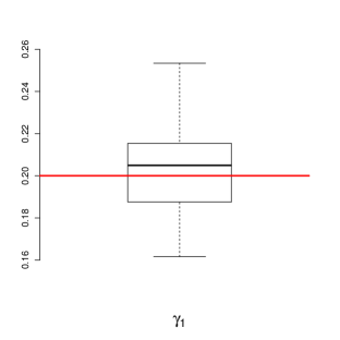
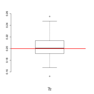
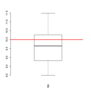
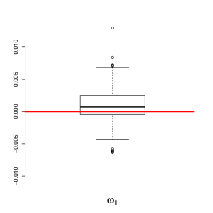
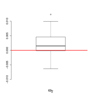
Figure 2: Summary of parameter estimates for Scenario A of the simulation study: boxplots of parameter estimates for $100$ simulated datasets.

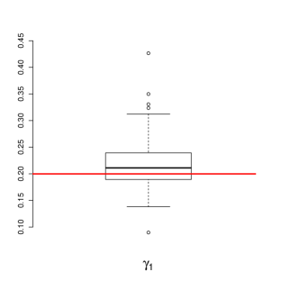
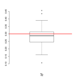
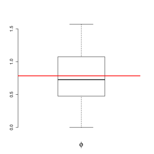
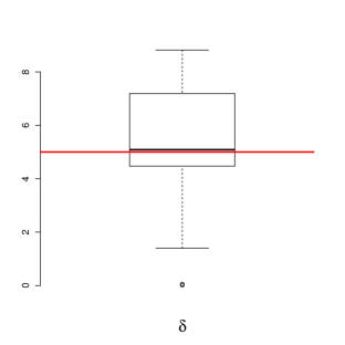
Figure 3: Summary of parameter estimates for Scenario B of the simulation study: boxplots of parameter estimates for $100$ simulated datasets.

Model parameters are estimated on $100$ data replications using the composite likelihood approach developed in Section 4. We have considered a larger number of replications for some parameter combinations, but in general the number of $100$ replications is enough to satisfactorily illustrate the estimation efficiency. The evaluation of $pl(\theta)$ depends on the choice of $\Delta_{S}$ and $\Delta_{T}$, where greater values increase the computational cost. Results in the literature indicate that using as much as computationally possible or all of the pairs will not necessarily lead to an improvement in estimation owing to potential issues with estimation variance (see Huser and Davison (2014), for instance). We have considered different values of $\Delta_{T}$ and have identified $\Delta_{T}=15$ as a good compromise for the estimation quality. The parameter $\Delta_{S}$ has been set to $1$ which is large enough with respect to the spatial domain limits. Main results are illustrated in the boxplots in Figures 2 and 3.

When the cylinder is circle-based, i.e. $\gamma_{1}=\gamma_{2}$, and without velocity (scenario A), the orientation parameter $\phi$ can take any value. In the simulation experiment we estimate all parameters without constraints, such that the optimization algorithm gives also an estimate of $\phi$. It is reassuring to see in the boxplots of Fig. 2 that the other parameters are still well estimated.

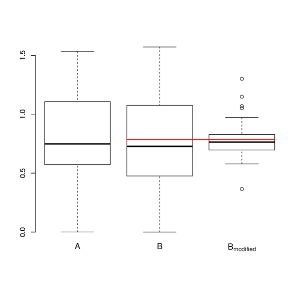
Figure 4: Parameter estimates of the simulation study: boxplots of $\phi$ estimates according to scenario A, scenario B and a modified scenario B with $\gamma_{2}=0.5$.

Results are fairly good for the scenario B where the velocity is non null. The estimates of the velocity present slightly higher variability, and the estimation of $\omega_{2}$ appears slightly biased. On the other hand, the duration $\delta$ and the lengths of the semi-axes of the ellipse ($\gamma_{1}$ and $\gamma_{2}$) are still well estimated. The angle $\phi$ is well defined in scenario B, but it is still estimated with relatively high variability. This may seem as disappointing at first glance, but it may be due to the only moderate difference in the length of the semi-axes. To check this conjecture, we consider a modified scenario B where the second semi-axis is modified from $\gamma_{2}=0.3$ to $\gamma_{2}=0.5$ and other parameters remain unchanged. As illustrated by the boxplots in Figure 4, estimation of $\phi$ clearly improves when the shape of the ellipse departs more strongly from a circular shape.

Even with only a relatively small number of spatial sites and time steps, the simulation study shows that the pairwise composite likelihood approach leads to reliable estimates of model parameters that are well identifiable. We underline that results are consistently good whatever the complexity of the scenario.

6 Space-time modeling of hourly precipitation data in southern France

6.1 Data

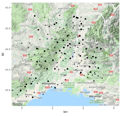
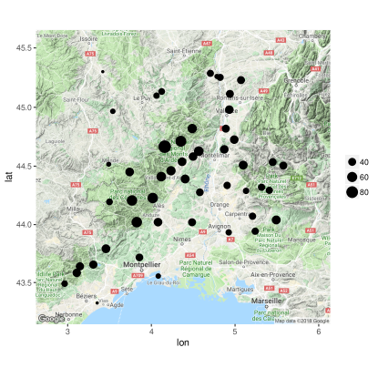
	$u$
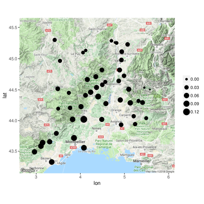
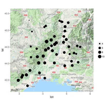
$\xi$	$\sigma$

Figure 5: Precipitation data of Southern France. Top left display: topographic map showing the meteorological stations selected for our case study. Dots correspond to the stations used for fitting. In the other displays, their diameter is proportional to empirical $99\%$ quantiles $u(s)$ (top right plot) and to estimates of the GPD parameters $\xi(s)$ (bottom left plot) and $\sigma(s)$ (bottom right plot).

We apply our hierarchical model to precipitation extremes observed over a study region in the South of France. Extreme rainfall events usually occur during fall season. They are mainly due to southern winds driving warm and moist air from the Mediterranean sea towards the relatively cold mountainous areas of the Cevennes and the Alps, leading to a situation which often provokes severe thunderstorms. The data were provided by Météo France (https://publitheque.meteo.fr). Our dataset is part of a query containing hourly observations at $213$ rainfall stations for years 1993 to 2014. To avoid modeling complex seasonal trends, we keep only data from the September to November months, resulting in observations over $54542$ hours. For model fitting, we consider a subsample of $50$ meteorological stations with elevations ranging from $2$ to $1418$ meters, for which the observation series contain less than $70\%$ of missing values over the full period. The spatial design of the stations is illustrated in Figure 5.

6.2 Exploratory analysis

We fit the univariate model (5) for each station by fixing a threshold $u$ that corresponds to the empirical $99\%$ quantile. We use such a rather high probability value since we have many observations, and there is a substantial number of zero values such that a high quantile is needed to get into the tail region of the positive values. Figure 5 clearly shows that spatial nonstationarity arises in the marginal distributions.

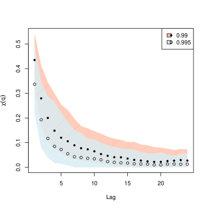
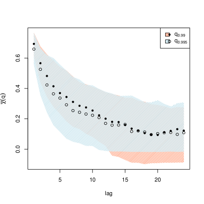
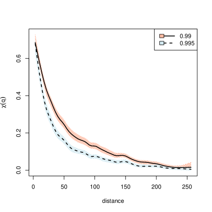
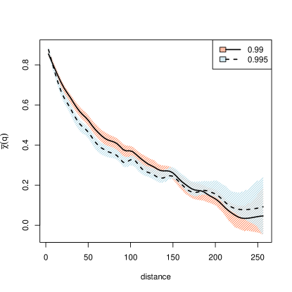
Figure 7: Empirical estimates of ${\chi}_{x}(q)$ (left panels) and ${\bar{\chi}}_{x}(q)$ (right panels) coefficients for the precipitation data. The filled region represents an approximate 95% confidence region based on a stationary bootstrap procedure.

Figure 7 displays the results of a bootstrap procedure in which we calculate estimates of $\chi(q)$ and $\bar{\chi}(q)$ for probabilities $q=0.99,0.995$ for pairs $Z(s,t)$, $Z(s,t+h)$ with only temporal lag, and for pairs $Z(s,t)$, $Z(s^{\prime},t)$ with only spatial lag. The curves for spatial lags are the result of a smoothing procedure. Confidence bands are based on $200$ bootstrap samples, drawn by the stationary bootstrap (Politis and Romano, 1994). Our procedure samples temporal blocks of observations and the block length follows a geometric distribution with an average of $20$ days. These plots support the assumption of asymptotic independence at all positive distances and at all positive temporal lags. Moreover, the strength of tail dependence as measured by the subasymptotic tail correlation value $\chi(q)$ strongly decreases when considering exceedances over increasingly high thresholds, which provides another clear sign of continuously decreasing and ultimately vanishing dependence strength. On the other hand, the values of the subasymptotic dependence measure $\overline{\chi}(q)$ (well adapted to asymptotic independence) decrease with increasing spatial distances or temporal lags, but they tend to stabilize at a non zero value. This behavior indicates the presence of residual tail dependence that vanishes only asymptotically.

6.3 Modeling spatio-temporal dependence

While the preceding exploratory analysis has shown that marginal distributions are not stationary, our model detailed in Section 2 requires a specific type of common marginal distributions. It would indeed be possible to extend the model to accommodate non stationary patterns (an example can be found in Bortot and Gaetan (2016)) and to jointly estimate marginal and dependence parameters. However, our focus here is to illustrate that our modeling strategy is capable to capture complex stationary spatio-temporal dependence patterns at large values, which would render joint estimation of margins and dependence highly intricate. Therefore, we fit a GP distribution separately to each site with thresholds chosen as the empirical $99\%$ quantile. With respect to positive precipitation, this quantile globally corresponds to a probability of $0.91$, with a minimum of $0.86$ and maximum of $0.95$ over the $50$ sites. Next, we use the estimated parameters $\hat{\xi}$ and $\hat{\sigma}$ to transform the raw exceedances $Y(x)$ observed at site $x$ to exceedances $\tilde{Y}(x)$ with cdf (5) such that $\xi=1$ and $\sigma=\kappa+1$, i.e.,

$$\tilde{Y}(x)=(\kappa+1)\left\{\left(1+\frac{\hat{\xi}\,Y(x)}{\hat{\sigma}}\right)^{1/\hat{\xi}}-1\right\}.$$

Since $\kappa$ must satisfy $\Pr(\tilde{Y}(x)>0)=(\kappa+1)^{-1}=0.01$, see Equation (6), we get $\kappa=99$.

We fit our hierarchical models to the censored pretransformed data $\tilde{Y}(x)$ by numerically maximizing the pairwise likelihood. We set the spatial cut-off distance to $\Delta_{S}=110\,km$, which retains about $60\%$ of the pairs of meteorological stations, and we choose the temporal cut-off as $\Delta_{T}=10$ hours. The resulting number of pairs of observations is approximately $4.6\times 10^{9}$, taking into account missing values. The full pairwise likelihood counts around $1.7\times 10^{11}$ pairs, which shows that we have attained a huge reduction. Pairwise likelihood maximization is coded in C, and it runs in parallel using the R library parallel. All calculations were carried out on a $2.6$ GHz machine with $32$ cores and $52Gb$ of memory. One evaluation of the composite likelihood requires approximately $18$ seconds. For calculating standard errors and CLIC^∗ values, we use the previously described subsampling technique based on temporal windows by considering $B=500$ overlapping blocks, each corresponding to $1000$ consecutive hours, i.e. $d_{b}=50\times 1000$.

We consider two settings for the hierarchical model, with (G1) and without velocity (G2). Then, we compare these two models to three variants of a censored Gaussian space-time copula model labeled C1, C2 and C3 (Bortot et al., 2000; Renard and Lang, 2007; Davison et al., 2013) pertaining to the class of asymptotic independent processes. The fits of the censored Gaussian space-time copula models match a censored Gaussian random field with transformed threshold exceedances; i.e., we transform original data to standard Gaussian margins $G(x)=\Phi^{\leftarrow}(\text{GP}(\tilde{Y}(x)))$ (with $\Phi$ the standard Gaussian cdf), and we suppose that $\{G(x),\,x\in\mathcal{X}\}$ is a Gaussian space-time random field with space-time correlation function $\rho(x_{1},x_{2};\theta)$.

We denote by $\rho_{e}(a)=\exp(-a)$ and by $\rho_{s}(a)=(1-1.5a+0.5a^{3})1_{[0,1]}(a)$, $a\geq 0$, the exponential and spherical correlation models with scale $1$, respectively. We introduce the scaled Mahalanobis distance between spatial locations $s_{1}$ and $s_{2}$, written

$$a(s_{1},s_{2};\tau)=\{(s_{1}-s_{2})^{\prime}\Omega(\tau)^{-1}(s_{1}-s_{2})\}^{1/2}$$

where

$$\Omega(\tau)=\left(\begin{array}[]{cc}\cos(\tau_{1})&-\sin(\tau_{1})\\ \sin(\tau_{1})&\cos(\tau_{1})\\ \end{array}\right)\left(\begin{array}[]{cc}1&0\\ 0&\tau_{2}^{-1}\\ \end{array}\right)\left(\begin{array}[]{cc}\cos(\tau_{1})&\sin(\tau_{1})\\ -\sin(\tau_{1})&\cos(\tau_{1})\\ \end{array}\right).$$

The Mahalanobis distance defines elliptical isocontours. Here, $\tau_{1}\in[0,\pi)$ is the angle with respect to the West-East direction, and $\tau_{2}>0$ is the length ratio of the two principal axes. We choose three specifications of the space-time correlation function:

• Space-time separable model:

  $$\rho(x_{1},x_{2};\theta)=\rho_{e}(a(s_{1},s_{2};\tau)/\psi_{S})\,\rho_{e}(|t_{1}-t_{2}|/\psi_{T})$$ (12)

  with $\theta=(\tau_{1},\tau_{2},\psi_{S},\psi_{T})$. We assume anisotropic spatial correlation in analogy to models G1 and G2. The model is isotropic for $\tau_{2}=1$.

• Frozen field model 1 (see Christakos, 2017, for a comprehensive account):

  $$\rho(x_{1},x_{2};\theta)=\rho_{e}(a(s_{1}-\nu t_{1},s_{2}-\nu t_{2};\tau)/\psi)$$ (13)

  where $\theta=(\tau_{1},\tau_{2},\psi,\nu^{\prime})$ and $\nu\in\mathbb{R}^{2}$ is a velocity vector.

• Frozen field model 2 with compact support:

  $$\rho(x_{1},x_{2};\theta)=\rho_{s}(a(s_{1}-\nu t_{1},s_{2}-\nu t_{2};\tau)/\psi).$$ (14)

  In this model, two observations separated by Mahalonobis distance $a(s_{1}-\nu t_{1},s_{2}-\nu t_{2};\tau)$ greater than $\psi$ will be independent.

Evaluation of the full likelihood of the models C1, C2 and C3 requires numerical operations such as matrix inversion, matrix determinants and high-dimensional Gaussian cdfs (Genz and Bretz, 2009), which are computationally intractable in our case. Therefore, we opt again for a pairwise likelihood approach, which also simplifies model selection through the CLIC^∗.

Estimation results are summarized in Table 2. The CLIC^∗ in the last column shows a preference for our hierarchical models with the best value for model G1, followed closely by G2. Estimated durations vary only slightly between G1 and G2. Estimates of $\phi$ differ more strongly, but one has to take into account that estimates of both semi-axis are very close. Moreover, estimates of $\gamma_{1}$ and $\gamma_{2}$ are similar for G1 and G2, which suggests coherent results for the two models and allows reliable physical interpretation of estimated parameter values. Regarding the results for model G1, we observe that the estimated parameters $\gamma_{1}$ and $\gamma_{2}$ characterize an ellipse covering a large part of the study region, which indicates relatively strong dependence even between sites that are far separated in space.

The estimate of $\phi$ underlines the low inclination of the ellipse, while $\gamma_{2}\approx 2\,\gamma_{1}$, which leads to an ellongated shape of the ellipse. It corresponds well to the orientation of the mountain ridges in the considered region.

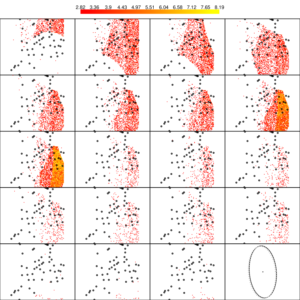
Figure 6: A simulation example showing exceedances of the $0.95$-quantile for the model G1 fitted to precipitation data. Dots correspond to the stations used for fitting. The evolution over time during $19$ hours is presented row-wise starting from the top left. The bottom right display illustrates the estimated ellipses, centred at the barycenter of the locations, and the movement induced by the velocity vector.

The estimate of $\delta$, which may be interpreted as the average duration of extreme events, correponds well to empirical measures of the actual durations of extreme events in the study region. The orientation of the reliefs seems to play an important role for the estimated velocity characterized by the values of $\omega_{1}$ and $\omega_{2}$, with $\omega_{1}$ being considerably larger than $\omega_{2}$. For visual illustration, Figure 6 shows a simulation of model G1 where the velocity effect in precipitation intensities becomes apparent. This simulation shows heavy precipitation arriving from the north, predominantly spreading over the eastern slopes of a mountain range in the study region, and then becoming more intense and finally gradually evacuating towards the south.

Among the Gaussian copula models, the preference goes to the separable model C1.

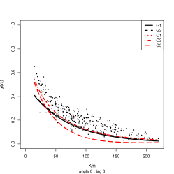
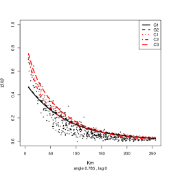
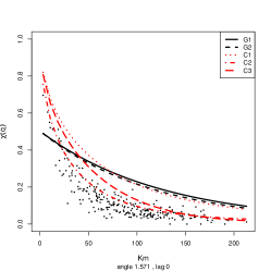
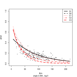
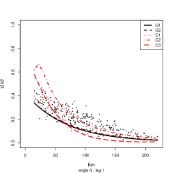
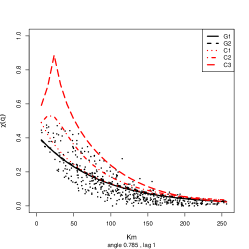
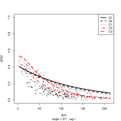
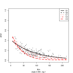
Figure 8: Estimated probabilities $\Pr(Z(s,t)>q|Z(s^{\prime},t^{\prime})>q)$ along different directions (expressed in radians) and at different temporal lags for the precipitation data. Dotted points correspond to empirical estimates. The value $q$ is fixed to the empirical $99\%$ quantile.

To underpin the good fit of our models through visual diagnostics, Figure 8 shows estimated probabilities $\Pr(Z(s,t)>q|Z(s^{\prime},t^{\prime})>q)$ along different directions and at different temporal lags $|t-t^{\prime}|$. These plots suggest that the behavior of models G1 and G2 is very close; there is no strong preference for one model over the other. The ranking of the copula models based on the CLIC^∗ is also confirmed by the visual diagnostics. For contemporaneous observations with time lag $0$, the models C1, C2 and C3 have comparable performance in capturing spatial dependence. However, for lags of $1$ hour, models C2 and C3 represent the space-time interaction not satisfactorily.

Finally, we gain deeper insight into the joint tail structure of the fitted models by calculating empirical estimates $\hat{p}_{i}(h)$ of the multivariate conditional probability

$$\chi^{*}_{s_{i};h}(q):=\Pr(Z(s_{j},t)>q,s_{j}\in\partial s_{i}|Z(s_{i},t-h)>q)$$

where $\partial s_{i}$ is the set of the four nearest neighbors of site $s_{i}$, $i=1,\ldots,50$. We compare these values with precise Monte-Carlo estimates $\tilde{p}_{i}^{(j)}(h)$, $j=1,\ldots,200$, based on a parametric bootstrap procedure using $200$ simulations of the models G1, G2 and C1 with the leading CLIC^∗ values. We compute site-specific root mean squared errors (RMSE)

$$\mathrm{RMSE}_{i}(h)=\left\{\frac{\sum_{j=1}^{200}(\tilde{p}^{(j)}_{i}(h)-\hat{p}_{i}(h))^{2}}{200}\right\}^{1/2},$$

as well as the resulting total RMSE, $\mathrm{RMSE}(h)=\sum_{i=1}^{50}\mathrm{RMSE}_{i}(h)$, as an overall measure of goodness of fit. Table 3 reports such values for fitted models using contemporaneous observations or lags of $1$ or $2$ hours ($h=0,1,2$) between the reference site and its neighbors. If we consider the quantile $q_{0.99}$ used as a threshold for fitting models, our hierarchical models present the best fit in terms of RMSE only for lagged values. However, models G1 and G2 extrapolate better for larger values of the threshold such as $q_{0.995}$.

7 Conclusions

We have proposed a novel space-time model for threshold exceedances of data with asymptotically vanishing dependence strength. In the spirit of the hierarchical modeling paradigm with latent layers to capture complex dependence and time dynamics, it is based on a latent Gamma convolution process with nonseparable space-time indicator kernels, and therefore amenable to physical interpretation. This framework leads to marginal and joint distributions that are available in closed form and are easy to handle in the extreme value context. The assumption of conditional independence as in our model is practical since it avoids the need to calculate cumulative distribution functions in large dimensions, although difficulty remains in evaluating the volume of the intersections of more than two cylinders and in calculating partial derivates for full likelihood formula. We can draw an interesting parallel to the max-stable Reich-Shaby process $Z_{RS}(x)$ (Reich and Shaby, 2012), which is one of the more easily tractable spatial max-stable models and has a related construction. Indeed, the inverted process $1/Z_{RS}(x)$ can be represented as the embedding of a dependent latent convolution process (based on positive $\alpha$-stable variables) for the rate of an exponential distribution. Conditional independence models cannot accurately capture the smoothness of the data generating process. Nevertheless, the $\alpha$-parameter in our model of the Gamma noise in (8) partially controls the smoothness of the latent Gamma field $\Lambda(s)$, with smaller values yielding more rugged surfaces.

In cases where data present asymptotic dependence, our asymptotically independent model may substantially underestimate the probability of jointly observing very high values over several space-time points. Asymptotic dependence in our construction (4) is equivalent to lower tail dependence in $\Lambda(x)$. There is no natural choice for introducing such dependence behavior, but a promising idea is to use what we label Beta scaling: given a temporal process $B(t)$ independent of $\Lambda(s,t)$ with $\mathrm{Beta}(\tilde{\alpha},\alpha)$ distributed margins, $0<\tilde{\alpha}<\alpha$, we could replace $\Lambda(s,t)$ in our construction by the process $\tilde{\Lambda}(s,t)=B(t)\Lambda(s,t)$ possessing margins following the $\Gamma(\tilde{\alpha},\beta)$ distribution. This construction has asymptotic dependence over space, and it will be asymptotically dependent over time if $B(t)$ has lower tail dependence. Follow-up work will explore theoretical properties and practical implementation of such extensions.

We have developed pairwise likelihood inference for our models, which scales well with high-dimensional datasets. We point out that handling observations over irregular time steps and missing data is straightforward with our model thanks to its definition over continuous time. While we think that MCMC-based Bayesian estimation of the relatively high number of parameters may be out of reach principally due to the very high dimension of the set of latent Gamma variables in the model’s current formulation, we are confident that future efforts to tackle the conditional simulation of such space-time processes based on MCMC simulation with fixed parameters could be successful; i.e., by using frequentist estimation of parameters, space-time prediction requires to iteratively update only the latent Gamma field through MCMC, but not parameters.

The application of our novel model to a high-dimensional real precipitation dataset from southern France was motivated from clear evidence of asymptotic independence highlighted at an exploratory stage. It provides practical illustration of the high flexibility of our model and its capability to accurately predict extreme event probabilities for concomitant threshold exceedances in space and time. Based on meteorological knowledge about the precipitation processes in the study region, we had hoped to estimate a clear velocity effect. As a matter of fact, the fitted hierarchical model with velocity appeared to be only slightly superior to other models in some aspects. This interesting finding may also be interpreted as evidence for the highly fragmented structure arising in precipitation processes at small spatial and temporal scales.

Ongoing work aims to adapt the current latent process construction to the multivariate setting by considering constructions with Gamma factors common to several components, specifically structures with a hierarchical tree-based construction of the latent Gamma components, and extensions to asymptotic dependence using the above-mentioned Beta-scaling. Ultimately, such novelties could provide a flexible toolbox for multivariate space-time modeling with scenarios of partial or full asymptotic dependence.

8 Appendix 1 : formulas for the Laplace exponent of a random measure

The Laplace exponent of the random measure $\Gamma(\cdot)$ is defined as

$$\mathcal{L}(\phi):=-\log\mathrm{E}\left(\exp\left\{-\int\phi(x)\Gamma(dx)\right\}\right)=\int_{\mathcal{X}}\log\left\{1+\frac{\phi(x)}{\beta}\right\}\alpha(dx),$$

where $\phi$ is any positive measurable function.
Consider $\phi=v\mathbf{1}_{A}(x)$. Then,

$$\mathcal{L}(\phi)=-\log\mathrm{E}\left(\exp\{-v\Gamma(A)\}\right)=\int_{A}\log\left\{1+\frac{v}{\beta}\right\}\alpha(dx)=\alpha(A)\log\left\{1+\frac{v}{\beta}\right\},$$

i.e.,

$$\mathrm{E}\left(\exp\{-v\Gamma(A)\}\right)=\left(\frac{\beta}{v+\beta}\right)^{\alpha(A)}.$$

For bivariate analyses, choosing $\phi(x)=v_{1}\mathbf{1}_{A_{1}}(x)+v_{2}\mathbf{1}_{A_{2}}(x)$, yields

$$\mathcal{L}(\phi) = -\log\mathrm{E}\left(\exp\{-v_{1}\Gamma(A_{1})-v_{2}\Gamma(A_{2})\}\right)$$

$$= -\log\mathrm{E}\left(\exp\{-v_{1}\Gamma(A_{1}\backslash A_{2})-(v_{1}+v_{2})\Gamma(A_{1}\cap A_{2})-v_{2}\Gamma(A_{2}\backslash A_{1})\}\right)$$

$$= \int_{A_{1}\backslash A_{2}}\log\left\{1+\frac{v_{1}}{\beta}\right\}\alpha(dx)+\int_{A_{1}\cap A_{2}}\log\left\{1+\frac{v_{1}+v_{2}}{\beta}\right\}\alpha(dx)$$

$$+\int_{A_{2}\backslash A}\log\left\{1+\frac{v_{2}}{\beta}\right\}\alpha(dx)$$

$$= \alpha(A_{1}\backslash A_{2})\log\left\{1+\frac{v_{1}}{\beta}\right\}+\alpha(A_{1}\cap A_{2})\log\left\{1+\frac{v_{1}+v_{2}}{\beta}\right\}+\alpha(A_{2}\backslash A_{1})\log\left\{1+\frac{v_{2}}{\beta}\right\}$$

and therefore

$$\mathrm{E}(\exp\{-v_{1}\Gamma(A_{1})-v_{2}\Gamma(A_{2})\})=\left(1+\frac{v_{1}}{\beta}\right)^{-\alpha(A_{1}\backslash A_{2})}\left(1+\frac{v_{1}+v_{2}}{\beta}\right)^{-\alpha(A_{1}\cap A_{2})}\left(1+\frac{v_{2}}{\beta}\right)^{-\alpha(A_{2}\backslash A_{1})}.$$

9 Appendix 2 : Formulas for the pairwise censored likelihood

Let $LP^{(1)}(v)$ and $LP_{x,x^{\prime}}^{(2)}(v_{1},v_{2})$, $x\neq x^{\prime}$ denote the univariate and bivariate Laplace transform of $\Lambda(A_{x})$ i.e.,

$$LP^{(1)}(v):=\mathrm{E}\left(e^{-v\Lambda(A_{x})}\right)=\left(\frac{\beta}{v+\beta}\right)^{c_{0}},$$

and

$$LP_{x,x^{\prime}}^{(2)}(v_{1},v_{2}):=\mathrm{E}\left(e^{-v_{1}\Lambda(A_{x})-v_{2}\Lambda(A_{x^{\prime}})}\right)=\left(\frac{\beta}{v_{1}+\beta}\right)^{c_{1}}\left(\frac{\beta}{v_{1}+v_{2}+\beta}\right)^{c_{2}}\left(\frac{\beta}{v_{2}+\beta}\right)^{c_{3}}$$

with $c_{0}=\alpha(A_{x})$ $c_{1}=\alpha(A_{x}\backslash A_{x^{\prime}})$, $c_{2}=\alpha(A_{x}\cap A_{x^{\prime}})$, $c_{3}=\alpha(A_{x^{\prime}}\backslash A_{x})$.

We obtain

$$\frac{\partial}{\partial v}LP^{(1)}(v) = -c_{0}\beta^{c_{0}}(v+\beta)^{-c_{0}-1},$$

$$\frac{\partial}{\partial v_{1}}LP_{x,x^{\prime}}^{(2)}(v_{1},v_{2}) = -\beta^{c_{1}+c_{2}+c_{3}}\left\{c_{1}(v_{1}+\beta)^{-c_{1}-1}(v_{1}+v_{2}+\beta)^{-c_{2}}(v_{2}+\beta)^{-c_{3}}\right.$$

$$+\left.c_{2}(v_{1}+\beta)^{-c_{1}}(v_{1}+v_{2}+\beta)^{-c_{2}-1}(v_{2}+\beta)^{-c_{3}}\right\},$$

$$\frac{\partial}{\partial v_{2}}LP_{x,x^{\prime}}^{(2)}(v_{1},v_{2}) = -\beta^{c_{1}+c_{2}+c_{3}}\left\{c_{3}(v_{1}+\beta)^{-c_{1}}(v_{1}+v_{2}+\beta)^{-c_{2}}(v_{2}+\beta)^{-c_{3}-1}\right.$$

$$+\left.c_{2}(v_{1}+\beta)^{-c_{1}}(v_{1}+v_{2}+\beta)^{-c_{2}-1}(v_{2}+\beta)^{-c_{3}}\right\},$$

$$\frac{\partial}{\partial v_{1}\partial v_{2}}LP_{x,x^{\prime}}^{(2)}(v_{1},v_{2}) = \beta^{c_{1}+c_{2}+c_{3}}\left\{c_{1}c_{2}(v_{1}+\beta)^{-c_{1}-1}(v_{1}+v_{2}+\beta)^{-c_{2}-1}(v_{2}+\beta)^{-c_{3}}\right.$$

$$+\left.c_{1}c_{3}(v_{1}+\beta)^{-c_{1}-1}(v_{1}+v_{2}+\beta)^{-c_{2}}(v_{2}+\beta)^{-c_{3}-1}\right.$$

$$+\left.c_{2}(c_{2}+1)(v_{1}+\beta)^{-c_{1}}(v_{1}+v_{2}+\beta)^{-c_{2}-2}(v_{2}+\beta)^{-c_{3}}\right.$$

$$+\left.c_{2}c_{3}(v_{1}+\beta)^{-c_{1}}(v_{1}+v_{2}+\beta)^{-c_{2}-1}(v_{2}+\beta)^{-c_{3}-1}\right\}.$$

	Parameters
Scenario	$\gamma_{1}$	$\gamma_{2}$	$\phi$	$\delta$	$\omega_{1}$	$\omega_{2}$
A	0.2	0.2	-	10	0.00	0.00
B	0.2	0.3	$\pi/4$	5	0.05	0.10

Table 1: Design of the two simulation scenarios.

Model	Parameters
	$\gamma_{1}$	$\gamma_{2}$	$\phi$	$\delta$	$\omega_{1}$	$\omega_{2}$	CLIC∗
G1	165.062	318.823	0.085	20.184	0.723	0.446	404480.8
	23.459	19.811	0.026	0.948	0.195	0.009
G2	175.817	294.323	0.041	20.036	0	0	404488.1
	11.879	25.291	0.064	1.039	-	-
C1	$\tau_{1}$	$\tau_{2}$	$\psi_{S}$	$\psi_{T}$			CLIC∗
	0.057	2.568	137.692	10.128			404626.2
	0.060	0.309	7.615	0.523
	$\tau_{1}$	$\tau_{2}$	$\psi_{S}$		$\nu_{1}$	$\nu_{2}$	CLIC∗
C2	1.034	2.025	108.755		6.672	16.358	404750.3
	0.040	0.318	7.299		0.908	1.502
C3	0.481	5.125	174.980		6.614	10.406	405020.4
	0.005	0.262	6.955		0.095	0.226

Table 2: Estimates, standard errors (in italic) and CLIC^∗ values of fitted models. Parameter units are kilometers for $\phi_{S}$, $\gamma_{1}$ and $\gamma_{2}$, radians for $\phi$ and $\tau_{1}$, hours for $\delta$ and $\phi_{T}$ and kilometers per hour for $\omega_{1}$, $\omega_{2}$, $\nu_{1}$ and $\nu_{2}$.

	$\mathrm{RMSE}(0)$		$\mathrm{RMSE}(1)$		$\mathrm{RMSE}(2)$
	$q_{0.99}$	$q_{0.995}$	$q_{0.99}$	$q_{0.995}$	$q_{0.99}$	$q_{0.995}$
G1	2.614	2.096	1.901	1.643	1.475	1.496
G2	2.605	2.072	1.907	1.626	1.477	1.480
C1	2.240	2.455	2.053	2.428	1.779	1.928

Table 3: Total root mean squared errors for the estimates of $\chi^{*}_{s_{i};h}(q)$.

(a)	(b)

Figure 1: Space-time kernels. Left display: a spatial ellipse $E(s,\gamma_{1},\gamma_{2},\phi)$ centered at $s$. Right display: an intersection of two slated elliptical cylinders $A_{s,t}$ and $A_{s^{\prime},t^{\prime}}$ with duration $\delta$.

References

- (1)
- Bacro et al. (2016) Bacro, J. N., Gaetan, C., and Toulemonde, G. (2016), “A flexible dependence model for spatial extremes,” Journal of Statistical Planning and Inference, 172, 36–52.
- Barndorff-Nielsen et al. (2014) Barndorff-Nielsen, O. E., Lunde, A., Shepard, N., and Veraat, A. E. D. (2014), “Integer-valued trawl processes: A class of stationary infinitively divisible processes,” Scandinavian Journal of Statistics, 41, 693–724.
- Bevilacqua et al. (2012) Bevilacqua, M., Gaetan, C., Mateu, J., and Porcu, E. (2012), “Estimating space and space-time covariance functions: a weighted composite likelihood approach,” Journal of the American Statistical Association, 107, 268–280.
- Bortot et al. (2000) Bortot, P., Coles, S., and Tawn, J. (2000), “The multivariate Gaussian tail model: an application to oceanographic data,” Journal of the Royal Statistical Society: Series C, 49, 31–49.
- Bortot and Gaetan (2014) Bortot, P., and Gaetan, C. (2014), “A latent process model for temporal extremes,” Scandinavian Journal of Statistics, 41, 606–621.
- Bortot and Gaetan (2016) Bortot, P., and Gaetan, C. (2016), “Latent process modelling of threshold exceedances in hourly rainfall series,” Journal of Agricultural, Biological, and Environmental Statistics, 21, 531–547.
- Carlstein (1986) Carlstein, A. (1986), “The use of subseries values for estimating the variance of a general statistic from a stationary sequence,” The Annals of Statistics, 14, 1171–1179.
- Carreau and Bouvier (2016) Carreau, J., and Bouvier, C. (2016), “Multivariate density model comparison for multi-site flood-risk rainfall in the French Mediterranean area,” Stochastic Environmental Research Risk Assessement, 30, 1591–1612.
- Casson and Coles (1999) Casson, E., and Coles, S. G. (1999), “Spatial regression models for extremes,” Extremes, 1, 449–468.
- Christakos (2017) Christakos, G. (2017), Spatiotemporal Random Fields Theory and Applications, Amsterdam: Elsevier.
- Coles et al. (1999) Coles, S., Heffernan, J., and Tawn, J. (1999), “Dependence measures for extreme value analyses,” Extremes, 2, 339–365.
- Cooley et al. (2007) Cooley, D., Nychka, D., and Naveau, P. (2007), “Bayesian spatial modeling of extreme precipitation return levels,” Journal of the American Statistical Association, 102, 824–840.
- Cox and Isham (1988) Cox, D. R., and Isham, V. (1988), “A simple spatial-temporal model of rainfall,” Proceedings of the Royal Society of London A: Mathematical, Physical and Engineering Sciences, 415, 317–328.
- Davis et al. (2013a) Davis, R. A., Klüppelberg, C., and Steinkohl, C. (2013a), “Max-stable processes for modeling extremes observed in space and time,” Journal of the Korean Statistical Society, 42, 399–414.
- Davis et al. (2013b) Davis, R. A., Klüppelberg, C., and Steinkohl, C. (2013b), “Statistical inference for max-stable processes in space and time,” Journal of the Royal Statistical Society, 75, 791–819.
- Davis and Mikosch (2008) Davis, R. A., and Mikosch, T. (2008), “Extreme value theory for space-time processes with heavy-tailed distributions,” Stochastic Processes and their Applications, 118, 560–584.
- Davison and Gholamrezaee (2012) Davison, A. C., and Gholamrezaee, M. M. (2012), “Geostatistics of extremes,” Proceedings of the Royal Society London, Series A, 468, 581–608.
- Davison et al. (2013) Davison, A. C., Huser, R., and Thibaud, E. (2013), “Geostatistics of dependent and asymptotically independent extremes,” Journal of Mathematical Geosciences, 45, 511–529.
- Davison et al. (2012) Davison, A. C., Padoan, S. A., and Ribatet, M. (2012), “Statistical modelling of spatial extremes,” Statistical Science, 27, 161–186.
- de Haan and Ferreira (2006) de Haan, L., and Ferreira, A. (2006), Extreme Value Theory: an Introduction, New-York: Springer.
- Ferguson (1973) Ferguson, T. S. (1973), “A Bayesian analysis of some nonparametric p roblems,” The Annals of Statistics, 1, 209–230.
- Ferreira and de Haan (2014) Ferreira, A., and de Haan, L. (2014), “The generalized Pareto process; with a view towards application and simulation,” Bernoulli, 20, 1717–1737.
- Gaetan and Grigoletto (2007) Gaetan, C., and Grigoletto, M. (2007), “A hierarchical model for the analysis of spatial rainfall extremes,” Journal of Agricultural Biological and Environmental Statistics, 12, 434–449.
- Genz and Bretz (2009) Genz, A., and Bretz, F. (2009), Computation of Multivariate Normal and t Probabilities, New York, NY: Springer.
- Hughes and Chraibi (2012) Hughes, G. B., and Chraibi, M. (2012), “Calculating ellipse overlap areas,” Computing and Visualization in Science, 15, 291–301.
- Huser and Davison (2014) Huser, R., and Davison, A. C. (2014), “Space-time modelling of extreme events,” Journal of the Royal Statistical Society: Series B, 76, 439–461.
- Huser et al. (2017) Huser, R., Opitz, T., and Thibaud, E. (2017), “Bridging asymptotic independence and dependence in spatial extremes using gaussian scale mixtures,” Spatial Statistics, 21, 166–186.
- Huser et al. (2018) Huser, R., Opitz, T., and Thibaud, E. (2018), “Penultimate modeling of spatial extremes: statistical inference for max-infinitely divisible processes,” arXiv preprint arXiv:1801.02946, .
- Huser and Wadsworth (2018) Huser, R., and Wadsworth, J. L. (2018), “Modeling spatial processes with unknown extremal dependence class,” Journal of the American Statistical Association, pp. 1–11.
- Joe (1997) Joe, H. (1997), Multivariate Models and Dependence Concepts, London: Chapman & Hall.
- Kabluchko et al. (2009) Kabluchko, Z., Schlather, M., and de Haan, L. (2009), “Stationary max-stable fields associated to negative definite functions,” The Annals of Probability, 37, 2042–2065.
- Morris et al. (2017) Morris, S. A., Reich, B. J., Thibaud, E., and Cooley, D. (2017), “A space-time skew-t model for threshold exceedances,” Biometrics, 73, 749–758.
- Nieto-Barajas and Huerta (2017) Nieto-Barajas, L. E., and Huerta, G. (2017), “Spatio-temporal Pareto modelling of heavy-tail data,” Spatial Statistics, 20, 92–109.
- Noven et al. (2015) Noven, R. C., Veraart, A. E., and Gandy, A. (2015), “A latent trawl process model for extreme values,” arXiv preprint arXiv:1511.08190, .
- Opitz (2013) Opitz, T. (2013), “Extremal t processes: elliptical domain of attraction and a spectral representation,” Journal of Multivariate Analysis, 122, 409–413.
- Opitz (2016) Opitz, T. (2016), “Modeling asymptotically independent spatial extremes based on Laplace random fields,” Spatial Statistics, 16, 1–18.
- Opitz (2017) Opitz, T. (2017), “Spatial random field models based on Lévy indicator convolutions,” arXiv preprint arXiv:1710.06826, .
- Opitz et al. (2015) Opitz, T., Bacro, J.-N., and Ribereau, P. (2015), “The spectrogram: A threshold-based inferential tool for extremes of stochastic processes,” Electronic Journal of Statistics, 9, 842–868.
- Politis and Romano (1994) Politis, D. N., and Romano, J. P. (1994), “The stationary bootstrap,” Journal of the American Statistical Association, 89, 1303–1313.
- Reich and Shaby (2012) Reich, B. J., and Shaby, B. A. (2012), “A hierarchical max-stable spatial model for extreme precipitation,” The Annals of Applied Statistics, 6, 1430–1451.
- Reiss and Thomas (2007) Reiss, R., and Thomas, M. (2007), Statistical Analysis of Extreme Values, third edn, Basel: Birkhäuser.
- Renard and Lang (2007) Renard, B., and Lang, M. (2007), “Use of a Gaussian copula for multivariate extreme value analysis: Some case studies in hydrology,” Advances in Water Resources, 30, 897 – 912.
- Rodriguez-Iturbe et al. (1987) Rodriguez-Iturbe, I., Cox, D. R., and Isham, V. (1987), “Some models for rainfall based on stochastic point processes,” Proceedings of the Royal Society of London A: Mathematical, Physical and Engineering Sciences, 410, 269–288.
- Sang and Gelfand (2009) Sang, H., and Gelfand, A. (2009), “Hierarchical modeling for extreme values observed over space and time,” Environmental and Ecological Statistics, 16, 407–426.
- Schlather (2002) Schlather, M. (2002), “Models for stationary max-stable random fields,” Extremes, 5, 33–44.
- Sibuya (1960) Sibuya, M. (1960), “Bivariate extreme statistics,” Annals of the Institute of Statistical Mathematics, 11, 195–210.
- Smith (1990) Smith, R. L. (1990), “Max-stable processes and spatial extremes,” Preprint, University of Surrey.
- Tawn et al. (2018) Tawn, J., Shooter, R., Towe, R., and Lamb, R. (2018), “Modelling spatial extreme events with environmental applications,” Spatial Statistics, 28, 39–58.
- Thibaud et al. (2013) Thibaud, E., Mutzner, R., and Davison, A. C. (2013), “Threshold modeling of extreme spatial rainfall,” Water Resources Research, 49, 4633–4644.
- Thibaud and Opitz (2015) Thibaud, E., and Opitz, T. (2015), “Efficient inference and simulation for elliptical Pareto processes,” Biometrika, 102, 855–870.
- Varin and Vidoni (2005) Varin, C., and Vidoni, P. (2005), “A note on composite likelihood inference and model selection,” Biometrika, 52, 519–528.
- Wadsworth and Tawn (2012) Wadsworth, J., and Tawn, J. (2012), “Dependence modelling for spatial extremes,” Biometrika, 99, 253–272.
- Wolpert and Ickstadt (1998a) Wolpert, R. L., and Ickstadt, K. (1998a), “Poisson/gamma random fields for spatial statistics,” Biometrika, 85, 251–267.
- Wolpert and Ickstadt (1998b) Wolpert, R. L., and Ickstadt, K. (1998b), “Simulation of Lévy random fields,” in Practical Nonparametric and Semiparametric Bayesian Statistics, eds. D. Dey, P. Müller, and D. Sinha, New York, NY: Springer New York, pp. 227–242.