Successive Quadratic Upper-Bounding for Discrete Mean-Risk Minimization and Network Interdiction

Abstract.

The advances in conic optimization have led to its increased utilization for modeling data uncertainty. In particular, conic mean-risk optimization gained prominence in probabilistic and robust optimization. Whereas the corresponding conic models are solved efficiently over convex sets, their discrete counterparts are intractable. In this paper, we give a highly effective successive quadratic upper-bounding procedure for discrete mean-risk minimization problems. The procedure is based on a reformulation of the mean-risk problem through the perspective of its convex quadratic term. Computational experiments conducted on the network interdiction problem with stochastic capacities show that the proposed approach yields solutions within 1-2% of optimality in a small fraction of the time required by exact search algorithms. We demonstrate the value of the proposed approach for constructing efficient frontiers of flow-at-risk vs. interdiction cost for varying confidence levels.

Keywords: Risk, polymatroids, conic integer optimization, quadratic optimization, stochastic network interdiction.

July 2017; June 2018

 
BCOL RESEARCH REPORT 17.05
Industrial Engineering & Operations Research
University of California, Berkeley, CA 94720–1777

1. Introduction

Conic optimization problems arise frequently when modeling parametric value-at-risk (VaR) minimization, portfolio optimization, and robust optimization with ellipsoidal objective uncertainty. Although convex versions of these models are solved efficiently by polynomial interior-point algorithms, their discrete counterparts are intractable. Branch-and-bound and branch-and-cut algorithms require excessive computation time even for relatively small instances. The computational difficulty is exacerbated by the lack of effective warm-start procedures for conic optimization.

In this paper, we consider a reformulation of a conic quadratic discrete mean-risk minimization problem that lends itself to a successive quadratic optimization procedure benefiting from fast warm-starts and eliminating the need to solve conic optimization problems directly.

Let $u$ be an $n$-dimensional random vector and $x$ be an $n$-dimensional decision vector in a closed set $X\subseteq\mathbb{R}^{n}$. If $u$ is normally distributed with mean $c$ and covariance $Q$, the minimum value-at-risk for $u^{\prime}x$ at confidence level $1-\epsilon\$, i.e.,

$$\begin{split}\zeta(\epsilon)=\min\ &\bigg{\{}z:\operatorname{\mathbf{Prob}}\left(u^{\prime}x>z\right)\leq\epsilon,\ \ x\in X\bigg{\}},\end{split}$$

for $0<\epsilon\leq 0.5$, is computed by solving the mean-risk optimization problem

$$(\text{MR})\ \ \ \min\ \bigg{\{}c^{\prime}x+\Omega\displaystyle\sqrt{x^{\prime}Qx}:\ x\in X\bigg{\}},$$

where $\Omega=\Phi^{-1}(1-\epsilon)$ and $\Phi$ is the c.d.f. of the standard normal distribution [18]. If $u$ is not normally distributed, but its mean and variance are known, (MR) yields a robust version by letting $\Omega=\sqrt{(1-\epsilon)/\epsilon}$, which provides an upper bound on the worst-case VaR [16, 21]. Alternatively, if $u_{i}$’s are independent and symmetric with support $[c_{i}-\sigma_{i},c_{i}+\sigma_{i}]$, then letting $\Omega=\sqrt{\ln(1/\epsilon)}$ with $Q_{ii}=\sigma_{i}^{2}$ gives an upper bound on the worst-case VaR as well [13]. The reader is referred to Ben-Tal et al. [15] for an in-depth treatment of robust models through conic optimization. Hence, under various assumptions on the uncertainty of $u$, one arrives at different instances of the mean-risk model (MR) with a conic quadratic objective. Ahmed [1] studies the complexity and tractability of various stochastic objectives for mean-risk optimization. Maximization of the mean-risk objective is $\mathcal{N}P$-hard even for a diagonal covariance matrix [2, 5]. If $X$ is a polyhedron, (MR) is a special case of conic quadratic optimization [4, 28], which can be solved by polynomial-time interior points algorithm [3, 29, 14]. Atamtürk and Gómez [7] give simplex QP-based algorithms for this case.

The interest of the current paper is in the discrete case of (MR) with integrality restrictions: $X\subseteq\mathbb{Z}^{n}$, which is $\mathcal{N}P$-hard. Atamtürk and Narayanan [10] describe mixed-integer rounding cuts, and Çezik and Iyengar [19] give disjunctive cuts for conic mixed-integer programming. The integral case is more predominantly addressed in the special case of independent random variables over binaries. In the absence of correlations, the covariance matrix reduces to a diagonal matrix $Q=diag(q)$, where $q$ is the vector of variances. In addition, when the decision variables are binary, (MR) reduces to

$$(\text{DMR})\ \ \ \min\left\{c^{\prime}x+\Omega\sqrt{q^{\prime}x}:x\in X\subseteq\mathbb{B}^{n}\right\}\cdot$$

Several approaches are available for (DMR) for specific constraint sets $X$. Ishii et al. [25] give an $O(n^{6})$ algorithm when the feasible set $X$ is the set of spanning trees; Hassin and Tamir [22] utilize parametric linear programming to solve (DMR) when $X$ defines a matroid in polynomial time. Atamtürk and Narayanan [11] give a cutting plane algorithm utilizing the submodularity of the objective; Atamtürk and Jeon [9] extend it to the mixed 0-1 case with indicator variables. Atamtürk and Narayanan [12] give an $O(n^{3})$ algorithm over a cardinality constraint. Shen et al. [34] provide a greedy $O(n\log n)$ algorithm to solve the diagonal case over the unit hypercube. Nikolova [30] gives a fully polynomial-time approximation scheme (FPTAS) for an arbitrary set $X\subseteq\mathbb{B}^{n}$ provided the deterministic problem with $\Omega=0$ can be solved in polynomial time.

The reformulation we give in Section 2 reduces the general discrete mean-risk problem (MR) to a sequence of discrete quadratic optimization problems, which is often more tractable than the conic quadratic case [8]. The uncorrelated case (DMR) reduces to a sequence of binary linear optimization problems. Therefore, one can utilize the simplex-based algorithms with fast warm-starts for general constraint sets. Moreover, the implementations can benefit significantly for structured constraint sets, such as spanning trees, matroids, graph cuts, shortest paths, for which efficient algorithms are known for non-negative linear objectives.

A motivating application: Network interdiction with stochastic capacities

Our motivating problem for the paper is network interdiction with stochastic capacities; although, since the proposed approach is independent of the feasible set $X$, it can be applied to any problem with a mean-risk objective (MR).

The deterministic interdiction problem is a generalization of the classical min-cut problem, where an interdictor with a limited budget minimizes the maximum flow on a network by stopping the flow on a subset of the arcs at a cost per interdicted arc. Consider a graph $G=(N,A)$ with nodes $N$ and arcs $A$. Let $s$ be the source node and $t$ be the sink node. Let $\alpha_{a}$ be the cost of interdicting arc $a\in A$ and $\beta$ be the total budget for interdiction. Then, given a set $I$ of interdicted arcs, the maximum $s-t$ flow on the remaining arcs is the capacity of the minimum cut on the arcs $A\setminus I$. Wood [36] shows that the deterministic interdiction problem is $\mathcal{N}P$-hard and gives integer formulations for it. Royset and Wood [32] give algorithms for a bi-criteria interdiction problem and generate an efficient frontier of maximum flow vs. interdiction cost. Cormican et al. [20], Janjarassuk and Linderoth [26] consider a stochastic version of the problem, where interdiction success is probabilistic. Held et al. [23] develop a decomposition approach for interdiction when network topology is stochastic. Network interdiction is a dual counterpart of survivable network design [17, 31], where one installs capacity to maximize the minimum flow against an adversary blocking the arcs. See Smith et al. [35] for a review of network interdiction models and algorithms.

When the arc capacities are stochastic, we are interested in an optimal interdiction plan that minimizes the maximum flow-at-risk. Unlike the expectation criterion used in previous stochastic interdiction models, this approach provides a confidence level for the maximum flow on the arcs that are not interdicted. Letting $c$ be the mean capacity vector and $Q$ the covariance matrix, the mean-risk network interdiction problem is modeled as

$$\min\quad c^{\prime}x+\Omega\sqrt{x^{\prime}Qx}$$

s.t. $$By\leq x+z,$$

$$(\text{MRNI})\ \ \ \ \ \quad\quad \alpha^{\prime}z\leq\beta,$$

$$y_{s}=1,\ y_{t}=0,$$

$$x\in\{0,1\}^{A},y\in\{0,1\}^{N},z\in\{0,1\}^{A},$$

where $B$ is the node-arc incidence matrix of $G$. Here, $z_{a}$ is one if arc $a$ is interdicted at a cost of $\alpha_{a}$ and zero otherwise; and $x_{a}$ is one if arc $a$ is in the minimum mean-risk cut and zero otherwise. The optimal value of (MRNI) is the “flow-at-risk” for a given interdiction budget $\beta$. Note that when $\Omega=0$, (MRNI) reduces to the deterministic network interdiction model of Wood [36]; and, in addition, if $z$ is a vector of zeros, it reduces to the standard $s-t$ min-cut problem. In a recent paper Lei et al. [27] give a scenario-based approach stochastic network interdiction under conditional value-at-risk measure. The following example underlines the difference of interdiction solutions between deterministic and mean-risk models with stochastic capacities.

Example 1.

Consider the simple network in Figure 1 with two arcs from $s$ to $t$. Arc 1 has mean capacity 1 and 0 variance, whereas arc 2 has mean capacity 0.9 and variance $\sigma^{2}$. Suppose the budget allows a single-arc interdiction. Then, the deterministic model with $\Omega=0$ would interdict arc 1 with higher mean and leave arc 2 with high variance intact. Consequently, the maximum $s-t$ flow would exceed $0.9+0.5\sigma$ with probability 0.3085 according to the normal distribution. On the other hand, the mean-risk model with $\Omega>0.2$, interdicts arc 2 with lower mean, but high variance ensuring that the maximum $s-t$ flow to be no more than 1.

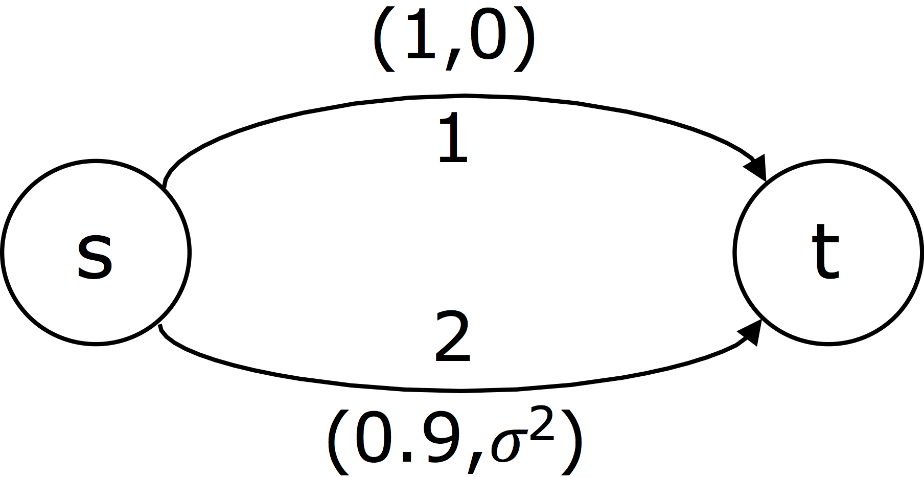
Figure 1. Mean-risk network interdiction.

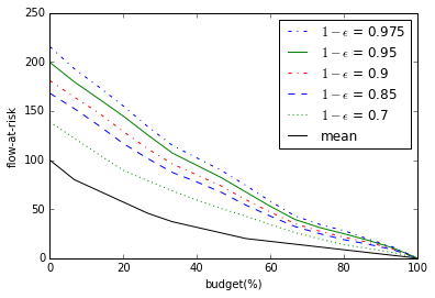
Figure 2. Flow-at-risk vs. interdiction budget for risk aversion levels.

The combinatorial aspect of network interdiction, coupled with correlations, make it extremely challenging to determine the least cost subset of arcs to interdict for a desired confidence level in the maximum flow even for moderate sized networks. Yet, understanding the cost and benefit of an interdiction strategy is of critical interest for planning purposes. Toward this end, the proposed approach in the current paper allows one to quickly build efficient frontiers of flow-at-risk vs. interdiction cost, which would, otherwise, be impractical for realistic sizes. Figure 2 shows the flow-at-risk as a function of the interdiction cost for different confidence levels for a $15\times 15$ grid graph shown in Figure 4. At 100% budget the network is interdicted completely allowing no flow. At lower budget levels the flow-at-risk increases significantly with the higher confidence levels. The vertical axis is scaled so that the deterministic min-cut value with $\Omega=0$ at 0% budget (no interdiction) is 100. The green solid curve corresponding to 95% confidence level shows that, if no interdiction is performed, the flow on the network is more than 200% of the deterministic maximum flow with probability 0.05. The same curve shows with 40% interdiction budget the flow is higher than the deterministic maximum flow (100) with probability only 0.05.

Contributions and outline

In Section 2, we give a non-convex upper-bounding function for (MR) that matches the mean-risk objective value at its local minima. Then, we describe an upper-bounding procedure that successively solves quadratic optimization problems instead of conic quadratic optimization. The rationale behind the approach is that algorithms for quadratic optimization with linear constraints scale better than interior point algorithms for conic quadratic optimization. Moreover, simplex algorithms for quadratic optimization can be effectively integrated into branch-and-bound algorithms and other iterative procedures as they allow fast warm-starts. In Section 3, we test the effectiveness of the proposed approach on the network interdiction problem with stochastic capacities and compare it with exact algorithms. We conclude in Section 4 with a few final remarks.

2. A successive quadratic optimization approach

In this section, we present a successive quadratic optimization procedure to obtain feasible solutions to (MR). The procedure is based on a reformulation of (MR) using the perspective function of the convex quadratic term $q(x)=x^{\prime}Qx$. Atamtürk and Gómez [7] introduce

$$(\text{PO})\ \ \ \min\left\{c^{\prime}x+\frac{\Omega}{2}h(x,t)+\frac{\Omega}{2}t:x\in X,\ t\geq 0\right\},$$

where $\Omega$ is a positive scalar as before, $h:\mathbb{R}^{n}\times\mathbb{R}_{+}\rightarrow\mathbb{R}\cup\{\infty\}$ is the closure of the perspective function of $q$ and is defined as

$$h(x,t):=\begin{cases}\frac{x^{\prime}Qx}{t}&\quad\text{ if }t>0,\\ 0&\quad\text{ if }t=0,\ x^{\prime}Qx=0,\\ +\infty&\quad\text{ otherwise. }\end{cases}$$

As the perspective of a convex function is convex [24], $h$ is convex. Atamtürk and Gómez [7] show the equivalence of (MR) and (PO) for a polyhedral set $X$. Since we are mainly interested in a discrete feasible region, we study (PO) for $X\subseteq\mathbb{Z}^{n}$.

For $t\geq 0$, it is convenient to define the optimal value function

$$f(t):=\underset{x\in X}{\min}\left\{g(x,t):=c^{\prime}x+\frac{\Omega}{2}h(x,t)+\frac{\Omega}{2}t\right\}\cdot$$ (1)

Given $t$, optimization problem (1) has a convex quadratic objective function. Let $x(t)$ be a minimizer of (1) with value $f(t)$. Note that $g$ is convex and $f$ is a point-wise minimum of convex functions in $t$ for each choice of $x\in X$, and is, therefore, typically non-convex (see Figure 3). We show below that, for any $t\geq 0$, $f(t)$ provides an upper bound on the mean-risk objective value for $x(t)$.

Lemma 1.

$\sqrt{a}\leq\frac{1}{2}(a/t+t)$ for all $a,t\geq 0$.

Proof.

Since $\sqrt{a}$ is concave over $a\geq 0$, it is bounded above by its gradient line:

$$\sqrt{a}\leq\sqrt{y}+\frac{1}{2\sqrt{y}}(a-y)$$

at any point $y\geq 0$. Letting $t=\sqrt{y}$ gives the result. ∎

Proposition 1.

For any $t\geq 0$, we have

$$c^{\prime}x(t)+\Omega\sqrt{{x(t)}^{\prime}Qx(t)}\leq f(t).$$

Proof.

Applying Lemma 1 with $a=x^{\prime}Qx\ (\geq 0\text{ as $Q$ is positive semidefinite})$ gives

$$\sqrt{x^{\prime}Qx}\leq\frac{1}{2}h(x,t)+\frac{t}{2},\ \forall x\in\mathbb{R}^{n},\ \forall t\geq 0.$$

First multiplying both sides by $\Omega\geq 0$ and then adding $c^{\prime}x$ shows

$$c^{\prime}x+\Omega\sqrt{x^{\prime}Qx} \leq c^{\prime}x+\frac{\Omega}{2}h(x,t)+\frac{\Omega}{2}t,\ \forall x\in\mathbb{R}^{n},\ \forall t\geq 0.$$

The inequality holds, in particular, for $x(t)$ as well. ∎

Example 2.

Consider the mean-risk optimization problem

$$\min\bigg{\{}x_{2}+\sqrt{10x_{1}^{2}+5x_{2}^{2}}:x\in X=\{(0,1),(1,0)\}\subseteq\mathbb{R}^{2}\bigg{\}}$$

with two feasible points. Figure 3 illustrates the optimal value function $f$. The curves in red and green show $g((1,0),t)$ and $g((0,1),t)$, respectively, and $f(t)=\min\{g((1,0),t),g((0,1),t)\}$ is shown with a dotted line. As the red and green curves intersect at $t=2.5$, $x(t)$ is $(0,1)$ for $t\leq 2.5$, and $(1,0)$ for $t\geq 2.5$.

In this example, $f$ has two local minima: $1+\sqrt{5}$ attained at $t=\sqrt{5}$ and $\sqrt{10}$ at $t=\sqrt{10}$. Observe that the upper bound $f(t)$ matches the mean-risk objective at these local minima:

$$c^{\prime}x({t})+\Omega\sqrt{x({t})^{\prime}Qx({t})}=f({t}),\ \ {t}\in\{\sqrt{5},\sqrt{10}\}.$$

The black step function shows the mean-risk values for the two feasible solutions of $X$. It turns out the upper bound $f(t)$ is tight, in general, for any local minima (Proposition 2).

In order to contrast the convex and discrete cases, we show with solid blue curve the lower bound $\hat{f}$ of $f$, where $\hat{f}(t)=\min\{g(x,t):x\in\hat{X}\}$ and $\hat{X}:=\{(x_{1},x_{2})\in\mathbb{R}^{2}_{+}:x_{1}+x_{2}=1\}$ is the convex relaxation of $X$. Let $\hat{x}(t)$ be the solution of this convex problem. Then $\hat{f}(t)$ provides an upper bound on $c^{\prime}\hat{x}(t)+\Omega\sqrt{{\hat{x}(t)}^{\prime}Q\hat{x}(t)}$ (graph shown in dotted blue curve) at any $t\geq 0$, and the bound is tight at $t=\sqrt{25/7}$, where the minimum of $\hat{f}(t)$ is attained.

Figure 3. The value function $f$ with two discrete feasible points.

Although, in general, $f(t)$ provides an upper bound, the next proposition shows that the mean-risk objective and $f$ match at local minima of $f$.

Proposition 2.

If $f$ has a local minimum at $\bar{t}>0$, then we have

$$c^{\prime}x(\bar{t})+\Omega\sqrt{{x(\bar{t})}^{\prime}Qx(\bar{t})}=f(\bar{t}).$$ (2)

Proof.

Since $f$ is the point-wise minimum of differentiable convex functions, it is differentiable at its local minima in the interior of its domain ($t>0$). Then, its vanishing derivative at $\bar{t}$

$$f^{\prime}(\bar{t})=-\frac{x(\bar{t})^{\prime}Qx(\bar{t})}{\bar{t}^{2}}+1=0$$

implies $\bar{t}=\sqrt{x(\bar{t})^{\prime}Qx(\bar{t})}$. Plugging this expression into $f(\bar{t})$ gives the result. ∎

Finally, we show that problems (MR) and (PO) are equivalent. In other words, the best upper bound matches the optimal value of the mean-risk problem, which provides an alternative way for solving (MR).

Proposition 3.

Problems (MR) and (PO) are equivalent; that is,

$${\min}\left\{c^{\prime}x+\Omega\sqrt{x^{\prime}Qx}:x\in X\right\}=\min\{f(t):t\geq 0\}\cdot$$

Proof.

Let $t^{*}$ be optimal for $\min\{f(t):t\geq 0\}$. By Proposition 1

$$f(t^{*})\geq c^{\prime}x(t^{*})+\Omega\sqrt{x(t^{*})^{\prime}Qx(t^{*})}\geq{\min}\left\{c^{\prime}x+\Omega\sqrt{x^{\prime}Qx}:x\in X\right\}.$$

The other direction follows from the observation

$$\min_{x\in X}\left\{c^{\prime}x+\Omega\sqrt{x^{\prime}Qx}\right\} =\min_{x\in X,\;{t\geq 0}}\left\{c^{\prime}x+\frac{\Omega}{2}\text{{h}{}}(x,t)+\frac{\Omega}{2}t:t=\sqrt{x^{\prime}Qx}\right\}$$

$$\geq\min_{x\in X,\;t\geq 0}\left\{c^{\prime}x+\frac{\Omega}{2}\text{{h}{}}(x,t)+\frac{\Omega}{2}t\right\}=\min_{t\geq 0}\{f(t)\}\cdot$$

∎

The one-dimensional upper-bounding function $f$ above suggests a local search algorithm that utilizes quadratic optimization to evaluate the function at any $t\geq 0$:

$$f(t)=\min_{x\in X}\left\{g(x,t):=c^{\prime}x+\frac{\Omega}{2t}x^{\prime}Qx+\frac{\Omega}{2}t\right\}$$

and avoids the solution of a conic quadratic optimization problem directly.

Algorithm 1 describes a simple binary search method that halves the uncertainty interval $[t_{min},t_{max}]$, initiated as $t_{min}=0$ and $t_{max}=\sqrt{\bar{x}^{\prime}Q\bar{x}}$, where $\bar{x}$ is an optimal solution to (MR) with $\Omega=0$. The algorithm is terminated either when a local minimum of $f$ is reached or the gap between the upper bound $f(t)$ and $c^{\prime}x(t)+\Omega\sqrt{x(t)^{\prime}Qx(t)}$ is small enough. For the computations in Section  3 we use 1% gap as the stopping condition.

Algorithm 1 Binary local search.

1:$X\subseteq\mathbb{Z}^{n};Q\text{ p.s.d. matrix; }c\text{ cost vector; }\Omega>0$

2:Local optimal solution $x$

3:Initialize $t_{\min}$ and $t_{\max}$

4:$\hat{z}\leftarrow\infty$ $\triangleright$ best objective value found

5:repeat

6:     $t\leftarrow\frac{t_{\min}+t_{\max}}{2}$

7:     $x(t)\leftarrow\operatorname*{arg\,min}\left\{c^{\prime}x+\frac{\Omega}{2t}x^{\prime}Qx+\frac{\Omega}{2}t:x\in X\right\}$   

8:     if $\frac{\partial g}{\partial t}(x(t),t)\leq-\epsilon$ then

9:         $t_{\min}\leftarrow t$

10:     else if  $\frac{\partial g}{\partial t}(x(t),t)\geq\epsilon$ then

11:         $t_{\max}\leftarrow t$

12:     else

13:         return $x(t)$

14:     end if

15:until stopping condition is met

16:return $\hat{x}$

The uncorrelated case over binaries

The reformulation (PO) simplifies significantly for the special case of independent random variables over binaries. In the absence of correlations, the covariance matrix reduces to a diagonal matrix $Q=diag(q)$, where $q$ is the vector of variances. For

$$(\text{DMR})\ \ \ \min\left\{c^{\prime}x+\Omega\sqrt{q^{\prime}x}:x\in X\subseteq\mathbb{B}^{n}\right\}$$

the upper bounding problem simplifies to

$$f(t)=\min\left\{c^{\prime}x+\frac{\Omega}{t}q^{\prime}x+\frac{\Omega}{2}t:x\in X\subseteq\mathbb{B}^{n}\right\},$$ (3)

which is a binary linear optimization problem for fixed $t$. Thus, $f$ can be evaluated fast for linear combinatorial optimization problems, such as the minimum spanning tree problem, shortest path problem, assignment problem, minimum cut problem [33], for which there exist polynomial-time algorithms. Even when the evaluation problem (3) is $\mathcal{N}P$-hard, simplex-based branch-and-bound algorithms equipped with warm-starts perform much faster than conic quadratic mean-risk minimization as demonstrated in the next section.

3. Computational Experiments

In this section we report on computational experiments conducted to test the effectiveness of the proposed successive quadratic optimization approach on the network interdiction problem with stochastic capacities. We compare the solution quality and the computation time with exact algorithms.

All experiments are carried out using CPLEX 12.6.2 solver on a workstation with a 3.60 GHz Intel R Xeon R CPU E5-1650 and 32 GB main memory and with a single thread. Default CPLEX settings are used with few exceptions: dynamic search and presolver are disabled to utilize the user cut callback; the branch-and-bound nodes are solved using linear outer approximation for faster enumeration; and the time limit is set to one hour.

Problem instances

We generate instances of the mean-risk network interdiction problem (MRNI) on grid graphs similar to the ones used in Cormican et al. [20], Janjarassuk and Linderoth [26]. Let $p\times q$ grid be the graph with $p$ columns and $q$ rows of grid nodes in addition to a source and a sink node (see Figure 4). The source and sink nodes are connected to all the nodes in the first and last column, respectively. The arcs incident to source or sink have infinite capacity and are not interdictable. The arcs between adjacent columns are always directed toward the sink, and the arcs connecting two nodes within the same column are directed either upward or downward with equal probability.

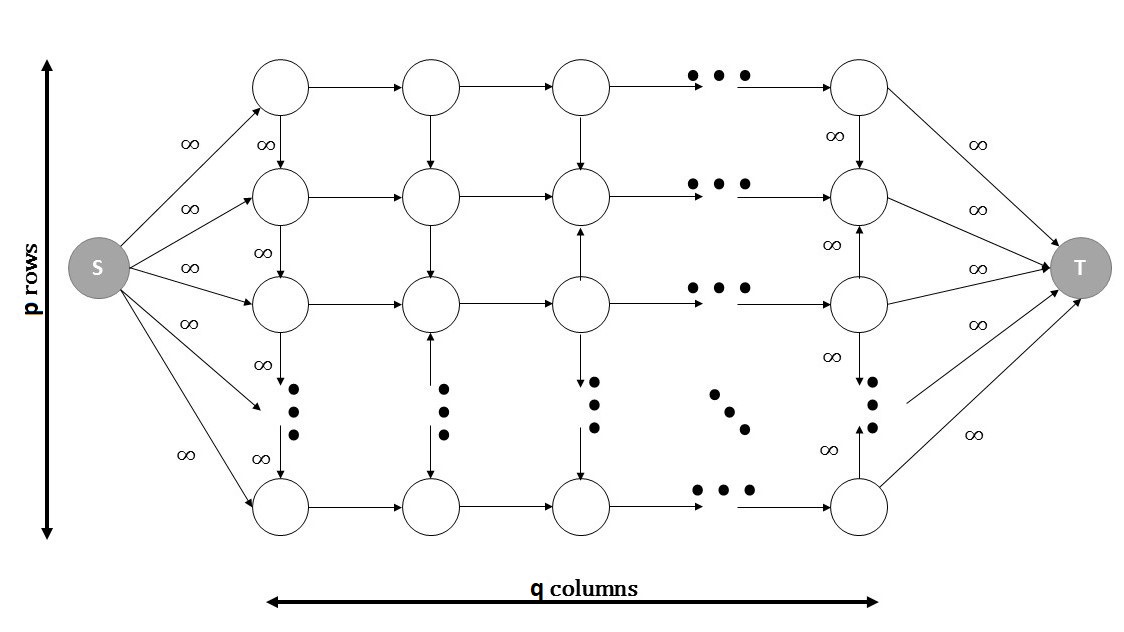
Figure 4. $p\times q$ grid graph.

We generate two types of data: uncorrelated and correlated. For each arc $a\in A$, the mean capacity $c_{a}$ and its standard deviation $\sigma_{a}$ are independently drawn from the integral uniform $[1,10]$, and the interdiction cost $\alpha_{a}$ is drawn from the integral uniform $[1,3]$. For the correlated case, the covariance matrix is constructed via a factor model: $Q=\operatorname{diag}(\sigma_{1}^{2},\cdots,\sigma^{2}_{|A|})+EFE^{\prime}$, where $F$ is an $m\times m$ factor covariance matrix and $E$ is the exposure matrix of the arcs to the factors. $F$ is computed as $F=HH^{\prime}$, where each $H_{ij}$ is drawn from uniform $[-100/pq,100/pq]$, and each $E_{ij}$ from uniform $[0,0.1]$ with probability 0.2 and set to 0 with probability 0.8. The interdiction budget $\beta$ is set to $\lceil\frac{Y}{2}\rceil$, and the risk averseness parameter $\Omega$ is set to $\Phi^{-1}(1-\epsilon)$, where $\Phi$ is the c.d.f. of the standard normal distribution. Five instances are generated for each combination of graph sizes $p\times q$ : $10\times 10$, $20\times 20$, $30\times 30$ and confidence levels $1-\epsilon$: 0.9, 0.95, 0.975. The data set is available for download at http://ieor.berkeley.edu/$\sim$atamturk/data/prob.interdiction .

For completeness, we state the corresponding perspective optimization for (MRNI):

$$\min\quad c^{\prime}x+\Omega x^{\prime}Qx/2t+\Omega t/2$$

s.t. $$By\leq x+z,$$

$$(\text{PO}-\text{MRNI})\ \ \ \ \ \quad\quad \alpha^{\prime}z\leq\beta,$$

$$y_{s}=1,\ y_{t}=0,$$

$$x\in\{0,1\}^{A},y\in\{0,1\}^{N},z\in\{0,1\}^{A},t\in\mathbb{R}_{+}.$$

Computations

Table 1 summarizes the performance of the successive quadratic optimization approach on the network interdiction instances. We present the number of iterations, the computation time in seconds, and the percentage optimality gap for the solutions, separately for the uncorrelated and correlated instances. Each row represents the average over five instances for varying grid sizes and confidence levels. One sees in the table that only a few number of iterations are required to obtain solutions within about 1% of optimality for both the correlated and uncorrelated instances. While the solution times for the correlated case are higher, even the largest instances are solved under 20 seconds on average. The computation time increases with the size of the grids, but is not affected by the confidence level $1-\epsilon$.

Table 1. Performance of the binary local search.

		Uncorrelated			Correlated
$p\times q$	$1-\epsilon$	iter	time	gap	iter	time	gap
$10\times 10$	0.9	2.8	0.04	1.47	3.0	0.10	0.68
	0.95	3.4	0.05	0.28	3.0	0.11	0.74
	0.975	2.8	0.05	0.00	3.0	0.09	0.73
$20\times 20$	0.9	3.0	0.49	1.54	4.0	2.74	0.35
	0.95	2.8	0.36	1.06	4.0	2.68	0.44
	0.975	2.8	0.45	1.07	4.0	3.21	5.86
$30\times 30$	0.9	3.0	2.24	1.67	5.0	16.00	0.46
	0.95	3.0	2.54	1.26	5.8	16.87	0.15
	0.975	3.0	2.58	1.19	5.8	18.57	0.20
avg		$\normalsize{\mathbf{2.96}}$	$\normalsize{\mathbf{0.98}}$	$\normalsize{\mathbf{1.06}}$	$\normalsize{\mathbf{4.18}}$	$\normalsize{\mathbf{6.71}}$	$\normalsize{\mathbf{1.07}}$

Table 2. Performance of b&b and b&c algorithms.

		Uncorrelated instances
		Cplex					Cplex $+$ cuts
$p\times q$	$1-\epsilon$	rgap	stime	time	egap (#)	nodes	cuts	rgap	stime	time	egap (#)	nodes
$10\times 10$	0.9	15.1	0	1	0.0	457	101	5.1	0	3	0.0	11
	0.95	17.0	1	1	0.0	1,190	127	5.6	2	4	0.0	75
	0.975	17.9	1	2	0.0	1,194	137	6.0	3	4	0.0	73
$20\times 20$	0.9	17.9	66	169	0.0	23,093	463	10.2	23	44	0.0	602
	0.95	20.0	469	676	0.0	56,937	579	11.4	48	102	0.0	4,850
	0.975	21.6	404	1,365	0.5(1)	91,786	621	12.5	79	262	0.0	16,883
$30\times 30$	0.9	19.1	2,338	3,258	4.6(4)	65,475	680	12.6	666	838	0.0	11,171
	0.95	21.3	3,315	3,600	10.3(5)	61,754	752	14.3	850	1,313	0.0	22,420
	0.975	23.1	3,535	3,600	15.3(5)	67,951	767	15.9	1,973	2,315	1.6(2)	35,407
avg		$\normalsize{\mathbf{19.2}}$	$\normalsize{\mathbf{1,125}}$	$\normalsize{\mathbf{1,408}}$	$\normalsize{\mathbf{3.4(15)}}$	$\normalsize{\mathbf{41,093}}$	$\normalsize{\mathbf{470}}$	$\normalsize{\mathbf{10.4}}$	$\normalsize{\mathbf{404}}$	$\normalsize{\mathbf{543}}$	$\normalsize{\mathbf{0.2(2)}}$	$\normalsize{\mathbf{10,166}}$
		Correlated instances
		Cplex					Cplex $+$ cuts
$p\times q$	$1-\epsilon$	rgap	stime	time	egap (#)	nodes	cuts	rgap	stime	time	egap (#)	nodes
$10\times 10$	0.9	10.5	2	4	0.0	268	114	5.8	4	7	0.0	14
	0.95	14.5	1	2	0.0	727	126	8.0	2	6	0.0	44
	0.975	16.2	2	2	0.0	1,105	120	10.3	2	5	0.0	67
$20\times 20$	0.9	15.0	49	92	0.0	11,783	341	12.0	26	31	0.0	1,199
	0.95	16.9	75	314	0.0	30,536	400	13.8	48	81	0.0	3,567
	0.975	18.2	802	615	0.0	66,759	420	15.1	66	129	0.0	6,911
$30\times 30$	0.9	12.1	427	873	0.0	21,748	343	9.3	130	246	0.0	4,325
	0.95	13.3	527	1,436	0.0	37,448	420	10.3	249	295	0.0	4,559
	0.975	13.8	1,776	2,465	0.4(1)	59,202	529	10.8	673	810	0.0	12,093
avg		$\normalsize{\mathbf{14.5}}$	$\normalsize{\mathbf{386}}$	$\normalsize{\mathbf{666}}$	$\normalsize{\mathbf{0.1(1)}}$	$\normalsize{\mathbf{25,509}}$	$\normalsize{\mathbf{313}}$	$\normalsize{\mathbf{10.6}}$	$\normalsize{\mathbf{133}}$	$\normalsize{\mathbf{179}}$	$\normalsize{\mathbf{0.0\phantom{0)}}}$	$\normalsize{\mathbf{3,642}}$

The optimal/best known objective values used for computing the optimality gaps in Table 1 are obtained with the CPLEX branch-and-bound algorithm. To provide a comparison with the successive quadratic optimization procedure, we summarize the performance for the exact algorithm in Table 2, for the uncorrelated and correlated instances, respectively. In each column, we report the percentage integrality gap at the root node (rgap), the time spent until the best feasible solution is obtained (stime), the total solution time in CPU seconds (time), the percentage gap between the best upper bound and the lower bound at termination (egap), and the number of nodes explored (nodes). If the time limit is reached before proving optimality, the number of instances unsolved (#) is shown next to egap. Each row of the tables represents the average for five instances.

Observe that the solution times with the CPLEX branch-and-bound algorithm are much larger compared to the successive quadratic optimization approach: 1,408 secs. vs. 1 sec. for the uncorrelated instances and 666 secs. vs. 7 secs. for the correlated instances. The difference in the performance is especially striking for the 30 $\times$ 30 instances, of which half are not solved to optimality within the time limit. Many of these unsolved instances are terminated with large optimality gaps (egap).

In order to strengthen the convex relaxation of 0-1 problems with a mean-risk objective, one can utilize the polymatroid inequalities [6]. Polymatroid inequalities exploit the submodularity of the mean-risk objective for the diagonal case. They are extended for the (non-digonal) correlated case as well as for mixed 0-1 problems in [11]. To improve the performance of the exact algorithm, we also test it by adding the polymatroid cuts. It is clear in Table 2 that the polymatroid cuts have a very positive impact on the exact algorithm. The root gaps are reduced significantly with the addition of the polymatroid cuts. Whereas 16 of the instances are unsolved within the time limit with default CPLEX, all but two instances are solved to optimality when adding the cuts. Nevertheless, the solution times even with the cutting planes are much larger compared to the successive quadratic optimization approach: 543 secs. vs. 1 sec. for the uncorrelated case and 179 secs. vs. 7 secs. for the correlated case.

Branch-and-bound and branch-and-cut algorithms spend a significant amount of solution time to prove optimality rather than finding feasible solutions. Therefore, for a fairer comparison, it is also of interest to check the time to the best feasible solution, which are reported under the column stime in Table 2. The average time to the best solution is 1,125 and 386 seconds for the branch-and-bound algorithm and 404 and 133 seconds for the branch-and-cut algorithm for the uncorrelated and correlated cases, respectively. Figure 5 presents the progress of the incumbent solution over time for one of the $30\times 30$ instances. The vertical axis shows the distance to the optimal value (100%). The binary search algorithm finds a solution within 3% of the optimal under 3 seconds. It takes 1,654 seconds for the default branch-and-bound algorithm and 338 seconds for the branch-and-cut algorithm to find a solution at least as good.

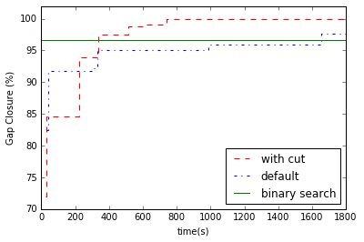
Figure 5. Performance profile of the algorithms.

The next set of experiments are done to test the impact of the budget constraint on the performance of the algorithms. For these experiments, the instances with $1-\epsilon=0.95$ and grid size $20\times 20$ are solved with varying levels of budgets. Specifically, the budget parameter $\beta$ is set to $\frac{\bar{\alpha}Y}{\eta}$ for $\eta\in\{2,4,6,8,10,20\}$, where $\bar{\alpha}$ denotes the mean value of $\alpha_{a}$. As before, each row of the Tables 3 – 4 presents the averages for five instances. Observe that the binary search algorithm is not as sensitive to the budget as the exact algorithms. For the exact the algorithms, while the root gap decreases with larger budget values, the solution time tends to increase, especially for the uncorrelated instances.

Table 3. Performance of the binary search for varying budgets.

	Uncorrelated			Correlated
$\eta$	iter	time	gap	iter	time	gap
2	3.0	0.30	0.00	4.0	1.33	0.27
4	2.8	0.36	1.06	4.0	2.68	0.44
6	2.8	0.38	1.02	4.0	1.70	0.54
8	3.0	0.35	0.17	4.0	1.69	0.26
10	3.0	0.36	0.03	4.0	1.48	1.50
avg	$\normalsize{\mathbf{2.92}}$	$\normalsize{\mathbf{0.35}}$	$\normalsize{\mathbf{0.46}}$	$\normalsize{\mathbf{4.0}}$	$\normalsize{\mathbf{1.78}}$	$\normalsize{\mathbf{0.60}}$

Table 4. Performance of b&b and b&c for varying budgets.

	Uncorrelated instances
	Cplex					Cplex $+$ cuts
$\eta$	rgap	stime	time	egap (#)	nodes	cuts	rgap	stime	time	egap (#)	nodes
2	24.4	3	6	0.0	680	104	7.1	7	8	0.0	18
4	20.0	469	676	0.0	56,937	579	11.4	48	102	0.0	4850
6	18.7	888	1,412	0.1(1)	123,930	626	11.5	94	124	0.0	6457
8	18.6	343	1,618	0.0	121,157	563	12.5	167	327	0.0	25,062
10	18.1	898	1,705	1.1(1)	121,624	523	12.3	225	300	0.0	21,130
avg	$\normalsize{\mathbf{20.0}}$	$\normalsize{\mathbf{520}}$	$\normalsize{\mathbf{1083}}$	$\normalsize{\mathbf{0.2(2)}}$	$\normalsize{\mathbf{84,865}}$	$\normalsize{\mathbf{479}}$	$\normalsize{\mathbf{10.9}}$	$\normalsize{\mathbf{108}}$	$\normalsize{\mathbf{172}}$	$\normalsize{\mathbf{0.0\phantom{(0)}}}$	$\normalsize{\mathbf{11,503}}$
	Correlated instances
	Cplex					Cplex $+$ cuts
$\eta$	rgap	stime	time	egap (#)	nodes	cuts	rgap	stime	time	egap (#)	nodes
2	25.4	6	11	0.0	1,325	128	19.8	3	9	0.0	125
4	16.9	75	314	0.0	30,536	400	13.8	48	81	0.0	3,567
6	13.4	86	246	0.0	32,990	408	10.6	43	94	0.0	7,574
8	13.2	105	199	0.0	27,514	386	10.9	38	62	0.0	4,997
10	12.3	37	129	0.0	20,880	330	9.8	33	35	0.0	1,870
avg	$\normalsize{\mathbf{16.2}}$	$\normalsize{\mathbf{61}}$	$\normalsize{\mathbf{180}}$	$\normalsize{\mathbf{0.0\phantom{(0)}}}$	$\normalsize{\mathbf{22,649}}$	$\normalsize{\mathbf{330}}$	$\normalsize{\mathbf{13.0}}$	$\normalsize{\mathbf{33}}$	$\normalsize{\mathbf{56}}$	$\normalsize{\mathbf{0.0\phantom{(0)}}}$	$\normalsize{\mathbf{3,627}}$

Next, we present the experiments performed to test the effect of the interdiction cost parameter $\alpha$. New instances with $1-\epsilon=0.95$ and grid size $20\times 20$ are generated with varying $\alpha_{a}$ drawn from integral uniform $[r,3r]$ for $r\in\{5,10,15,20,25\}$. To keep the relative scales of the parameters consistent with the previous experiments, the budget parameter $\beta$ is set to $\frac{\bar{\alpha}Y}{4}$. Tables 5 – 6 summarize the results. The optimality gaps for the binary search algorithm are higher for these experiments with similar run times. Both the binary search and the exact algorithms appear to be insensitive to the changes in the interdiction cost in our experiments.

Table 5. Performance of the binary search for varying interdiction costs.

	Uncorrelated			Correlated
$r$	iter	time	gap	iter	time	gap
5	3.0	0.39	3.93	4.0	2.15	0.22
10	2.8	0.42	1.94	4.0	2.05	4.29
15	2.8	0.41	3.43	4.0	2.17	0.48
20	2.8	0.41	1.20	4.0	2.24	0.80
25	2.8	0.44	1.76	4.0	2.22	0.63
avg	$\normalsize{\mathbf{2.84}}$	$\normalsize{\mathbf{0.41}}$	$\normalsize{\mathbf{2.45}}$	$\normalsize{\mathbf{4.0}}$	$\normalsize{\mathbf{2.17}}$	$\normalsize{\mathbf{1.29}}$

Table 6. Performance of b&b and b&c for varying interdiction costs.

	Uncorrelated instances
	Cplex					Cplex $+$ cuts
$r$	rgap	stime	time	egap (#)	nodes	cuts	rgap	stime	time	egap (#)	nodes
5	22.4	969	2,405	0.6(2)	299,432	705	15.1	296	428	0.0	26,404
10	22.5	1,299	2,552	1.8(2)	282,257	725	15.4	802	944	0.0	56,725
15	22.4	1,611	2,383	3.3(3)	267,595	686	15.3	815	1,319	0.5(1)	72,508
20	22.2	1,436	2,905	4.4(4)	279,349	704	14.9	336	775	0.0	44,972
25	22.3	1,502	2,905	4.2(4)	339,789	691	15.2	576	985	0.2(1)	57,971
avg	$\normalsize{\mathbf{22.4}}$	$\normalsize{\mathbf{1363}}$	$\normalsize{\mathbf{2630}}$	$\normalsize{\mathbf{2.8(15)}}$	$\normalsize{\mathbf{293,684}}$	$\normalsize{\mathbf{702}}$	$\normalsize{\mathbf{15.2}}$	$\normalsize{\mathbf{565}}$	$\normalsize{\mathbf{890}}$	$\normalsize{\mathbf{0.1(2)}}$	$\normalsize{\mathbf{51,716}}$
	Correlated instances
	Cplex					Cplex $+$ cuts
$r$	rgap	stime	time	egap (#)	nodes	cuts	rgap	stime	time	egap (#)	nodes
5	16.7	302	887	0.0	966,71	449	13.9	72	135	0.0	10,406
10	17.2	644	1,020	0.0	118,975	442	14.4	163	209	0.0	17,283
15	17.0	175	1,359	0.5(1)	124,748	434	14.2	91	157	0.0	13,486
20	16.9	800	1,434	0.0	140,953	418	14.0	57	263	0.0	21,663
25	16.7	379	1,276	0.0	140,621	440	13.8	108	200	0.0	16,675
avg	$\normalsize{\mathbf{16.9}}$	$\normalsize{\mathbf{460}}$	$\normalsize{\mathbf{1195}}$	$\normalsize{\mathbf{0.1(1)}}$	$\normalsize{\mathbf{124393}}$	$\normalsize{\mathbf{436}}$	$\normalsize{\mathbf{14.0}}$	$\normalsize{\mathbf{98}}$	$\normalsize{\mathbf{193}}$	$\normalsize{\mathbf{0.0\phantom{(0)}}}$	$\normalsize{\mathbf{15,902}}$

Finaly, we test the performance of the binary search algorithm for larger grid sizes up to $100\times 100$ to see how it scales up. Five instances of each size are generated as in our original set of instances. The exact algorithms are not run for these large instances; therefore, the gap is computed against the convex relaxation of the problem and, hence, it provides an upper bound on the optimality gap. Table 7 reports the number of iterations, the time spent for the algorithm, and the percentage integrality gap, that is the gap between the upper bound found by the algorithm and the lower bound from the convex relaxation.

Observe that the $100\times 100$ instances have about 20,000 arcs. The correlated instances for this size could not be run due to memory limit. For the $20\times 20$ instances, the reported upper bounds 20.73% and 17.31% on the optimality gap should be compared with the actual optimality gaps 1.06% and 0.44% in Table 1. The large difference between the exact gap in Table 1 and igap in Table 7 is indicative of poor lower bounds from the convex relaxations, rather than poor upper bounds. The binary search algorithm converges in a small number of iterations for these large instances as well; however, solving quadratic 0-1 optimization problems at each iteration takes significantly longer time.

Table 7. Performance of the binary local search for larger networks.

	Uncorrelated			Correlated
$p\times q$	iter	time	igap	iter	time	igap
$20\times 20$	2.8	0.36	20.73	4.0	2.68	17.31
$40\times 40$	3.0	5.33	26.15	5.0	80.47	11.81
$60\times 60$	3.2	35.66	27.09	6.0	502.14	10.12
$80\times 80$	3.6	141.96	27.31	6.0	3,199.11	8.53
$100\times 100$	10.2	4,991.3	31.08	-	-	-
avg	$\normalsize{\mathbf{4.6}}$	$\normalsize{\mathbf{1,034.92}}$	$\normalsize{\mathbf{26.47}}$	$\normalsize{\mathbf{5.3}}$	$\normalsize{\mathbf{945.97}}$	$\normalsize{\mathbf{11.94}}$

4. Conclusion

In this paper we introduce a successive quadratic optimization procedure embedded in a bisection search for finding high quality solutions to discrete mean-risk minimization problems with a conic quadratic objective. The search algorithm is applied on a non-convex upper-bounding function that provides tight values at local minima. Computations with the network interdiction problem with stochastic capacities indicate that the proposed method finds solutions within 1–4% optimal in a small fraction of the time required by exact branch-and-bound and branch-and-cut algorithms. Although we demonstrate the approach for the network interdiction problem with stochastic capacities, since method is agnostic to the constraints of the problem, it can be applied to any 0-1 optimization problem with a mean-risk objective.

References

- Ahmed [2006] S. Ahmed. Convexity and decomposition of mean-risk stochastic programs. Mathematical Programming, 106:433–446, 2006.
- Ahmed and Atamtürk [2011] S. Ahmed and A. Atamtürk. Maximizing a class of submodular utility functions. Mathematical Programming, 128:149–169, 2011.
- Alizadeh [1995] F. Alizadeh. Interior point methods in semidefinite programming with applications to combinatorial optimization. SIAM Journal on Optimization, 5:13–51, 1995.
- Alizadeh and Goldfarb [2003] F. Alizadeh and D. Goldfarb. Second-order cone programming. Mathematical Programming, 95:3–51, 2003.
- Atamtürk and Gómez [2017] A. Atamtürk and A. Gómez. Maximizing a class of utility functions over the vertices of a polytope. Operations Research, 65:433–445, 2017.
- Atamtürk and Gómez [2017] A. Atamtürk and A. Gómez. Submodularity in conic quadratic mixed 0-1 optimization. arXiv preprint arXiv:1705.05918, 2017. BCOL Research Report 16.02, IEOR, UC Berkeley.
- Atamtürk and Gómez [2017] A. Atamtürk and A. Gómez. Simplex QP-based methods for minimizing a conic quadratic objective over polyhedra. arXiv preprint arXiv:1706.05795, 2017. BCOL Research Report 17.02, IEOR, UC Berkeley.
- Atamtürk and Gómez [2018] A. Atamtürk and A. Gómez. Strong formulations for quadratic optimization with m-matrices and indicator variables. Mathematical Programming, 170:141–176, 2018.
- Atamtürk and Jeon [2017] A. Atamtürk and H. Jeon. Lifted polymatroid inequalities for mean-risk optimization with indicator variables. arXiv preprint arXiv:1705.05915, 2017. BCOL Research Report 17.01, IEOR, UC Berkeley.
- Atamtürk and Narayanan [2007] A. Atamtürk and V. Narayanan. Cuts for conic mixed integer programming. In M. Fischetti and D. P. Williamson, editors, Proceedings of the 12th International IPCO Conference, pages 16–29, 2007.
- Atamtürk and Narayanan [2008] A. Atamtürk and V. Narayanan. Polymatroids and mean-risk minimization in discrete optimization. Operations Research Letters, 36:618–622, 2008.
- Atamtürk and Narayanan [2009] A. Atamtürk and V. Narayanan. The submodular 0-1 knapsack polytope. Discrete Optimization, 6:333–344, 2009.
- Ben-Tal and Nemirovski [2000] A. Ben-Tal and A. Nemirovski. Robust solutions of linear programming problems contaminated with uncertain data. Mathematical Programming, 88:411–424, 2000.
- Ben-Tal and Nemirovski [2001] A. Ben-Tal and A. Nemirovski. Lectures on modern convex optimization: analysis, algorithms, and engineering applications. SIAM, 2001.
- Ben-Tal et al. [2009] A. Ben-Tal, L. El Ghaoui, and A. Nemirovski. Robust optimization. Princeton University Press, 2009.
- Bertsimas and Popescu [2005] D. Bertsimas and I. Popescu. Optimal inequalities in probability theory: A convex optimization approach. SIAM Journal on Optimization, 15:780–804, 2005.
- Bienstock and Muratore [2000] D. Bienstock and G. Muratore. Strong inequalities for capacitated survivable network design problems. Mathematical Programming, 89:127–147, 2000.
- Birge and Louveaux [2011] J. R. Birge and F. Louveaux. Introduction to Stochastic Programming. Springer, 2011.
- Çezik and Iyengar [2005] M. T. Çezik and G. Iyengar. Cuts for mixed 0-1 conic programming. Mathematical Programming, 104:179–202, 2005.
- Cormican et al. [1998] K. J. Cormican, D. P. Morton, and R. K. Wood. Stochastic network interdiction. Operations Research, 46:184–197, 1998.
- Ghaoui et al. [2003] L. E. Ghaoui, M. Oks, and F. Oustry. Worst-case value-at-risk and robust portfolio optimization: A conic programming approach. Operations Research, 51:543–556, 2003.
- Hassin and Tamir [1989] R. Hassin and A. Tamir. Maximizing classes of two-parameter objectives over matroids. Mathematics of Operations Research, 14:362–375, 1989.
- Held et al. [2005] H. Held, R. Hemmecke, and D. L. Woodruff. A decomposition algorithm applied to planning the interdiction of stochastic networks. Naval Research Logistics, 52:321–328, 2005.
- Hiriart-Urruty and Lemaréchal [2013] J.-B. Hiriart-Urruty and C. Lemaréchal. Convex analysis and minimization algorithms I: Fundamentals. Springer, 2013.
- Ishii et al. [1981] H. Ishii, S. Shiode, T. Nishida, and Y. Namasuya. Stochastic spanning tree problem. Discrete Applied Mathematics, 3:263–273, 1981.
- Janjarassuk and Linderoth [2008] U. Janjarassuk and J. Linderoth. Reformulation and sampling to solve a stochastic network interdiction problem. Networks, 52:120–132, 2008.
- Lei et al. [2018] Xiao Lei, Siqian Shen, and Yongjia Song. Stochastic maximum flow interdiction problems under heterogeneous risk preferences. Computers & Operations Research, 90:97–109, 2018.
- Lobo et al. [1998] M. S. Lobo, L. Vandenberghe, S. Boyd, and H. Lebret. Applications of second-order cone programming. Linear Algebra & its Applications, 284:193–228, 1998.
- Nesterov and Todd [1998] Y. E Nesterov and M. J. Todd. Primal-dual interior-point methods for self-scaled cones. SIAM Journal on Optimization, 8:324–364, 1998.
- Nikolova [2009] E. Nikolova. Strategic Algorithms. PhD thesis, Massachusetts Institute of Technology, 2009.
- Rajan and Atamtürk [2002] D. Rajan and A. Atamtürk. Survivable network design : Routing of flows and slacks. In G. Anandalingam and S. Raghavan, editors, Telecommunications Network Design and Management, pages 65–81. Kluwer Academic Publishers, 2002.
- Royset and Wood [2007] J. O. Royset and R. K. Wood. Solving the bi-objective maximum-flow network-interdiction problem. INFORMS Journal on Computing, 19:175–184, 2007.
- Schrijver [2003] Alexander Schrijver. Combinatorial optimization: polyhedra and efficiency, volume 24. Springer Science & Business Media, 2003.
- Shen et al. [2003] Z.-J. M. Shen, C. Coullard, and M. S. Daskin. A joint location-inventory model. Transportation Science, 37:40–55, 2003.
- Smith et al. [2013] J. C. Smith, M. Prince, and J. Geunes. Modern network interdiction problems and algorithms. In P. M. Pardalos, D.-Z. Du, and R. L. Graham, editors, Handbook of Combinatorial Optimization, pages 1949–1987. Springer, 2013.
- Wood [1993] R. K. Wood. Deterministic network interdiction. Mathematical and Computer Modelling, 17:1–18, 1993.