Dynamical system for animal coat pattern model

Abstract

We construct a dynamical system for a reaction diffusion system due to Murray, which relies on the use of the Thomas system nonlinearities and describes the formation of animal coat patterns. First, we prove existence and uniqueness of global positive strong solutions to the system by using semigroup methods. Second, we show that the solutions are continuously dependent on initial values. Third, we show that the dynamical system enjoys exponential attractors whose fractal dimensions can be estimated. Finally, we give a numerical example.

1 Introduction

We consider a model of animal coat patterns given by Murray ([8, 9]):

$$\begin{cases}\begin{aligned} &\frac{\partial u}{\partial t}=\Delta u+\gamma\Big{(}a-u-\frac{\rho uv}{1+u+ku^{2}}\Big{)}&\hskip 14.22636pt\text{ in }\Omega\times(0,\infty),\\ &\frac{\partial v}{\partial t}=\alpha\Delta v+\gamma\Big{\{}\beta(b-v)-\frac{\rho uv}{1+u+ku^{2}}\Big{\}}&\hskip 11.38092pt\text{ in }\Omega\times(0,\infty)\end{aligned}\end{cases}$$ (1.1)

in a bounded domain $\Omega\subset\mathbb{R}^{d}\,(d=1,2,3\dots)$. Here, $u(t)$ and $v(t)$ denote the concentration of the activator and inhibitor at time $t$, respectively. These concentrations are supplied at constant rates $\gamma a$ and $\gamma\beta b$, and are degrade linearly proportional to themselves. Furthermore, both are used up in the reaction at a rate $f(u,v)=\frac{\gamma\rho uv}{1+u+ku^{2}}.$ The form of $f(u,v)$ exhibits substrate inhibition, where $k$ is a measure of the severity of the inhibition. The constant $\alpha>1$ is the ratio of diffusion coefficient. The constant $\gamma$ is a measure of the domain size, which can have any of the following interpretations:

• $\gamma^{1/2}$ is proportional to the linear size of the spatial domain in one-dimension.

• $\gamma$ represents the relative strength of the reaction terms. This means, for example, that an increase in $\gamma$ may represent an increase in activity of some rate-limiting step in the reaction sequence.

• An increase in $\gamma$ can also be thought of as equivalent to a decrease in the diffusion coefficient ratio $\alpha$.

The system (1.1) is coupled with a Neumann boundary condition:

$$\begin{cases}\begin{aligned} &\frac{\partial u}{\partial\mathbf{n}}=\frac{\partial v}{\partial\mathbf{n}}=0&\hskip 28.45274pt\text{ on }\partial\Omega\times(0,\infty),\\ &u(0,x)=u_{0}\geq 0,v(0,x)=v_{0}\geq 0&\hskip 28.45274pt\text{ in }\Omega,\end{aligned}\end{cases}$$ (1.2)

where $\mathbf{n}$ denotes the exterior normal to the boundary $\partial\Omega.$

The system (1.1) is a special form of the activator-inhibitor system, which is general given by a reaction diffusion system

$$\begin{cases}\begin{aligned} &\frac{\partial u}{\partial t}=\alpha_{1}\Delta u+\gamma f(u,v)&\hskip 28.45274pt\text{ in }\Omega\times(0,\infty),\\ &\frac{\partial v}{\partial t}=\alpha_{2}\Delta v+\gamma g(u,v)&\hskip 28.45274pt\text{ in }\Omega\times(0,\infty).\end{aligned}\end{cases}$$ (1.3)

By the use of this model, one can obtain many pattern formations in biological, physical, or chemical systems. Gierer-Meinhardt ([3]) and Meinhardt ([7]) presented the functions

$$f=\nu_{1}-\nu_{2}u+\frac{\nu_{3}u^{2}}{v},$$

$$g=\nu_{4}u^{2}-\nu_{5}v$$

for a model of biological pattern formation. It is then called the Gierer-Meinhardt system. Global solutions to the system is then shown by Rothe ([10]). Existence of attractors and the Turing instability of the system are given by Yagi ([14]).

Masuda-Takahashi ([6]) then introduced a generalized Gierer-Meinhardt system, i.e. the system (1.3) with

$$f=\nu_{1}-\nu_{2}u+\frac{\nu_{3}u^{p}}{v^{q}},$$

$$g=\frac{\nu_{4}u^{r}}{v^{s}}-\nu_{5}v.$$

The authors then proved global existence of solutions in some special cases of coefficients. Li-Chen-Qin ([5]) and then Jiang ([4]) showed global existence of solutions in some other cases.

For the system (1.1), the nonlinearities came from the use of the Thomas system nonlinearities ([12]). Murray reproduced animal coat patterns from this model, and gave a heuristic explanation for the formation of these patterns by investigating the linearization of the system (1.1) at the unstable homogeneous stationary solution ([9]). He concluded that these patterns depend only on the eigenfunction corresponding to the largest eigenvalue of the linearization. Sander-Wanner then showed that the mechanism of these patterns is the same as that for spinodal decomposition in the Cahn-Hilliard equation ([1, 11]). This leads to a conclusion, which is in contrast to the Murray’s explanation that the patterns in spaces of dimension less than three can be explained by linear behaviour corresponding to a whole range of largest eigenvalues.

The above interesting results on the system (1.1) are based on an assumption: the system is well-posed. Not like to the Gierer-Meinhardt systems, global existence as well as existence of an attractor to (1.1) have not been investigated.

In this paper, we show that the system (1.1) coupled with (1.2) is well-posed. In other words, we prove existence and uniqueness of global positive strong solutions to (1.1), and show that the solution’s behavior changes continuously with initial conditions. For this, we use semigroup methods. We then construct a dynamical system for the model. Furthermore, by using the theory of dynamical systems (see Theorems 2.3 and 2.4) presented by Yagi ([14]), we show that the dynamical system enjoys exponential attractors whose fractal dimensions can be estimated.

The paper is organized as follows. Section 2 is preliminary. Some basic concepts such as sectorial operators, analytical semigroups, dynamical systems, and attractors are reviewed. In Section 3, we formulate the system (1.1) into an abstract form, and recall the definition of mild and strong solutions to the form. A sufficient condition for existence of strong solutions to the abstract equation is presented. In Section 4, we construct local strong solutions, and prove the nonnegativity of these solutions. Section 5 shows that the local strong solutions constructed in Section 4 are global by using a priori estimate for solutions. Section 6 provides the regular dependence of solutions on initial data. This helps us construct a continuous dynamical system in Section 7. Existence of exponential attractors is also shown in that section. The paper ends with a numerical example in Section 8.

2 Preliminary

Let $E$ be a Banach space with norm $\|\cdot\|$. Let us review concepts of analytical semigroups generated by sectorial operators in $E$, and of dynamical systems on $E$. For more details, see, e.g., [14].

Throughout this paper, Banach and Hilbert spaces are always defined over the complex field $\mathbb{C}$.

2.1 Sectorial operators and analytical semigroups

A densely defined, closed linear operator $A$ in $E$ is said to be sectorial if it satisfies the condition:

• The spectrum $\sigma(A)$ of $A$ is contained in an open sectorial domain $\Sigma_{\varpi}$:

  $$\sigma(A)\subset\Sigma_{\varpi}=\{\lambda\in\mathbb{C}:|\arg\lambda|<\varpi\},\quad\quad 0<\varpi<\frac{\pi}{2}.$$

  The resolvent of $A$ satisfies the estimate

  $$\|(\lambda-A)^{-1}\|\leq\frac{M_{\varpi}}{|\lambda|},\quad\quad\quad\quad\lambda\notin\Sigma_{\varpi}$$

  with some constant $M_{\varpi}>0$ depending only on the angle $\varpi$.

Let $A$ be a sectorial operator. The fractional powers $A^{\theta},-\infty<\theta<\infty,$ are then defined as follows. For each complex number $z$ such that ${\rm Re}\,z>0$, $A^{-z}$ is defined by using the Dunford integral in $\mathcal{L}(E)$:

$$A^{-z}=\frac{1}{2\pi i}\int_{\gamma}\lambda^{-z}(\lambda-A)^{-1}d\lambda.$$

Here, $\gamma=\gamma_{-}\cup\gamma_{0}\cup\gamma_{+}$ is an integral contour surrounding the spectrum $\sigma(A)$ counterclockwise in the domain $\mathbb{C}\setminus(-\infty,0]\cap\mathbb{C}\setminus\sigma(A)$ of the complex plane, where

$$\gamma_{\pm}\colon\lambda=\rho e^{\pm i\varpi},\hskip 56.9055pt\frac{\|A^{-1}\|^{-1}}{2}\leq\rho<\infty,$$

and

$$\gamma_{0}\colon\lambda=\frac{\|A^{-1}\|^{-1}}{2}e^{i\varphi},\hskip 28.45274pt-\varpi\leq\varphi\leq\varpi.$$

It is known that $A^{-z}$ is one to one for ${\rm Re}\,z>0$. The following definition is thus meaningful:

$$A^{z}=(A^{-z})^{-1}\hskip 28.45274pt\text{ for }{\rm Re}\,z>0.$$

In addition, it is natural to define $A^{0}=I$, the identity mapping on $E$. In this way, for every real number $-\infty<\theta<\infty,$ $A^{\theta}$ has been defined.

The following lemma shows useful estimates for fractional powers and the semigroup generated by a sectorial operator.

Lemma 2.1.

Let (H) be satisfied. Then,

• $(-A)$ generates an analytical semigroup $\{e^{-tA},t\geq 0\}.$

• For $0\leq\theta<\infty,$

  $$\|A^{\theta}e^{-tA}\|\leq\iota_{\theta}t^{-\theta},\hskip 56.9055pt0<t<\infty,$$ (2.1)

  where $\iota_{\theta}=\sup_{0\leq t<\infty}t^{\theta}\|A^{\theta}e^{-tA}\|<\infty$. In particular, there exists $0<\nu<\infty$ such that

  $$\|e^{-tA}\|\leq\iota_{0}e^{-\nu t}\leq\iota_{0},\hskip 56.9055pt0\leq t<\infty.$$ (2.2)

• For $0<\theta\leq 1,$

  $$\|[e^{-tA}-I]A^{-\theta}\|\leq\frac{\iota_{1-\theta}}{\theta}t^{\theta},\hskip 56.9055pt0\leq t<\infty.$$ (2.3)

For the proof, see [14].

2.2 Dynamical systems

A family of nonlinear operators $S(t),0\leq t<\infty$, from a subset $E_{0}$ of $E$ into $E_{0}$ is called a semigroup on $E_{0}$ if the family satisfies

• $S(0)=I$.

• $S(t)S(s)=S(t+s),\hskip 28.45274pt0\leq s,t<\infty$.

In addition to these properties, if the operators $S(t)$ satisfy

• $S(\cdot)(\cdot)$ is continuous from $[0,\infty)\times E_{0}$ to $E_{0}$

then the family is called a continuous semigroup on $E_{0}$.

Let $S$ be a continuous semigroup on $E_{0}$. For each $x\in E_{0}$, the trace of $E_{0}$ - valued continuous function $S(\cdot)x$ in $E_{0}$ is called a trajectory starting from $x$. A dynamical system is the set of trajectories starting from the points in $E_{0}$, and is denoted by a triple $(S,E_{0},E).$

A set $\mathcal{A}\subset E_{0}$ is called an absorbing set if $\mathcal{A}$ absorbs every bounded set of $E_{0}$, i.e. for any bounded set $B$ of $E_{0}$, there exists $0\leq t_{B}<\infty$ such that

$$S(t)B\subset\mathcal{A},\hskip 28.45274ptt_{B}\leq t<\infty.$$

A set $\mathcal{A}\subset E_{0}$ is called an attractor if it satisfies two conditions:

• $\mathcal{A}$ is an invariant set of the dynamical system, i.e.

  $$S(t)\mathcal{A}\subset\mathcal{A},\hskip 28.45274pt0\leq t<\infty.$$

• For some neighborhood $W$ of $\mathcal{A}$,

  $$\lim_{t\to\infty}h(S(t)W,\mathcal{A})=0.$$

  Here, $h(\cdot,\cdot)$ is the Hausdorff pseudo-distance, i.e. for two subsets $B_{1}$ and $B_{2}$ of $E$,

  $$h(B_{1},B_{2})=\sup_{x\in B_{1}}\inf_{y\in B_{2}}\|x-y\|.$$

An attractor $\mathcal{A}$ is called a global attractor of the dynamical system $(S,E_{0},E)$ if it satisfies three conditions:

• $\mathcal{A}$ is a compact set of $E.$

• $\mathcal{A}$ is a strictly invariant set of the dynamical system, i.e.

  $$S(t)\mathcal{A}=\mathcal{A},\hskip 28.45274pt0\leq t<\infty.$$

• $\lim_{t\to\infty}h(S(t)B,\mathcal{A})=0$ for every bounded set $B$ of $E_{0}$.

Let us finally review the concept of exponential attractors. A compact attractor $\mathcal{A}^{*}\subset E_{0}$ is called an exponential attractor if it satisfies the following conditions:

• $\mathcal{A}^{*}$ contains a global attractor $\mathcal{A}$ of the dynamical system $(S,E_{0},E).$

• $\mathcal{A}^{*}$ has finite fractal dimension. Here, the fractal dimension of $\mathcal{A}^{*}$ is defined by

  $$d_{F}(\mathcal{A}^{*})=-\limsup_{\epsilon\to 0}\frac{\log N(\epsilon)}{\log\epsilon},$$

  where $N(\epsilon)$ is the minimal number of balls with radius $\epsilon$ which cover the set $\mathcal{A}^{*}.$

• There exists $0<\alpha<\infty$ such that for all bounded set $B\subset E_{0}$,

  $$h(S(t)B,\mathcal{A}^{*})\leq C_{B}e^{-\alpha t},\hskip 28.45274pt0\leq t<\infty$$

  with some $0<C_{B}<\infty.$

Remark 2.2.

It is obvious that every dynamical system enjoys at most one global attractor. However, an exponential attractor, if it exists, is not unique in general. Exponential attractors exist as a family.

The following theorem shows a sufficient condition for existence of exponential attractors for a dynamical system.

Theorem 2.3.

Let $(S,E_{0},E)$ be a dynamical system in a Banach space $E$, where the phase space $E_{0}$ is a closed bounded set of $E$. Assume that there exist an operator $K$, two constants $0<t_{0}<\infty$ and $0\leq\delta<\frac{1}{2}$ satisfying the following conditions:

• $K\colon E_{0}\to E_{1}$, where $E_{1}$ is a Banach space which is compactly embedded in $E$. In addition, $K$ satisfies a Lipschitz condition in the sense

  $$\|K(x)-K(y)\|_{E_{1}}\leq L\|x-y\|,\hskip 28.45274ptx,y\in E_{0}$$

  with some $L>0.$

• $S(t_{0})$ is a compact perturbation of contraction operator in the sense

  $$\|S(t_{0})(x)-S(t_{0})(y)\|\leq\delta\|x-y\|+\|K(x)-K(y)\|,\hskip 28.45274ptx,y\in E_{0}.$$

• $S(\cdot)(\cdot)$ satisfies a Lipschitz condition on $[0,t_{0}]\times E_{0}$ in the sense

  $$\|S(t)(x)-S(s)(y)\|\leq L_{1}(|t-s|+\|x-y\|),\hskip 28.45274pt0\leq t,s\leq t_{0},x,y\in E_{0}$$

  with some $L_{1}>0.$

Then, for any $0<\theta<\frac{1-2\delta}{2L}$, there exists an exponential attractor $\mathcal{A}_{\theta}$ for $(S,E_{0},E)$ such that

$$h(S(t)E_{0},\mathcal{A}_{\theta})\leq\frac{R}{2(\delta+\theta L)}e^{\frac{t\log[2(\delta+\theta L)]}{t_{0}}},\hskip 28.45274pt0<t<\infty.$$

Here, $R$ is the diameter of $E_{0}$.

For the proof, see [14].

Let us now consider the case where $E$ is a Hilbert space and $E_{0}$ is a compact subset of $E$. We say that an operator $S_{1}$ from $E_{0}$ to $E_{0}$ has squeezing property if there exist a constant $0<\delta<\frac{1}{4}$ and an orthogonal operator $P$ of finite rank $N$ such that for $x,y\in E_{0}$, either

$$\|S_{1}(x)-S_{1}(y)\|\leq\delta\|x-y\|$$

or

$$(I-P)(S_{1}(x)-S_{1}(y))\leq\|P(S_{1}(x)-S_{1}(y))\|.$$

Theorem 2.4.

Let $(S,E_{0},E)$ be a dynamical system in a Hilbert space $E$, where $E_{0}\subset E$ is compact. Assume that for some fixed $0<t_{0}<\infty,$ the operator $S(t_{0})$ has the squeezing property with some $0<\delta<\frac{1}{4}$ and an orthogonal operator $P$ of finite rank $N.$ Assume further that $S(t)$ satisfies the Lipschitz condition (iii) of Theorem 2.3.

Then, for any $0<\theta<1-2\delta$, there exists an exponential attractor $\mathcal{A}_{\theta}$ for $(S,E_{0},E)$ such that

$$h(S(t)E_{0},\mathcal{A}_{\theta})\leq\frac{R}{2\delta+\theta}e^{\frac{t\log(2\delta+\theta)}{t_{0}}},\hskip 28.45274pt0<t<\infty.$$

In addition, the fractal dimension of $\mathcal{A}_{\theta}$ is finite and estimated by

$$d_{F}(A_{\theta})\leq 1+N\max\{-\frac{\log(\frac{3L_{1}}{\theta}+1)}{\log(2\delta+\theta)},1\}.$$

Here, $R$ is the diameter of $E_{0}$, i.e. $R=\sup_{x,y\in E_{0}}\|x-y\|.$

For the proof, see [14].

3 Abstract formulation

Let us formulate the system (1.1) coupled with the condition (1.2) as an abstract equation.

Set the underlying space

$$(E,\|\cdot\|)=(L_{2}(\Omega)\times L_{2}(\Omega),\|\cdot\|_{L_{2}\times L_{2}}),$$

where the norm is defined by $\Big{\|}\Big{(}\begin{matrix}x_{1}\\ x_{2}\end{matrix}\Big{)}\Big{\|}_{L_{2}\times L_{2}}=\sqrt{\|x_{1}\|_{L_{2}}^{2}+\|x_{2}\|_{L_{2}}^{2}},$ $\Big{(}\begin{matrix}x_{1}\\ x_{2}\end{matrix}\Big{)}\in E.$ And set the space of initial functions

$$V=\left\{\left(\begin{matrix}u_{0}\\ v_{0}\end{matrix}\right);0\leq u_{0},v_{0}\in L_{2}(\Omega)\right\}.$$ (3.1)

Denote by $A$ a diagonal matrix operator diag$\{A_{1},A_{2}\}$ of $E$, where $A_{1}$ and $A_{2}$ are realization of operators $-\Delta+\gamma$ and $-\alpha\Delta+\gamma\beta$ in $L_{2}(\Omega)$, respectively, under the homogeneous Neumann boundary condition (1.2) on $\partial\Omega$. According to [14, Theorem 1.25], $A_{i}\,(i=1,2)$ are positive define self-adjoint operators of $L_{2}(\Omega)$ with domain

$$\mathcal{D}(A_{i})=H^{2}_{N}(\Omega)=\{h\in H^{2}(\Omega);\frac{\partial h}{\partial\mathbf{n}}=0\text{ on }\partial\Omega\},$$

here $H^{2}(\Omega)$ denotes the space of all complex-valued functions whose partial derivatives in the distribution sense up to the second order belong to $L_{2}(\Omega).$ Furthermore, on account of [14, Theorem 16.7, 16.9], the domain of the fractional power $A^{\theta}$ is defined by

$$\mathcal{D}(A^{\theta})=\begin{cases}H^{2\theta}(\Omega)\times H^{2\theta}(\Omega),\hskip 28.45274pt\text{if }0\leq\theta<\frac{3}{4},\\ H^{2\theta}_{N}(\Omega)\times H^{2\theta}_{N}(\Omega),\hskip 28.45274pt\text{if }\frac{3}{4}<\theta\leq 1.\end{cases}$$ (3.2)

(Here,

$$H^{2\theta}_{N}(\Omega)=\{h\in H^{2\theta}(\Omega);\frac{\partial h}{\partial\mathbf{n}}=0\text{ on }\partial\Omega\},$$

and $H^{2\theta}(\Omega)$ is the space of all restrictions of functions in $H^{2\theta}(\mathbb{R}^{n})$ to $\Omega$. In addition,

$$H^{2\theta}(\mathbb{R}^{n})=\{f\in\mathcal{S}(\mathbb{R}^{n})^{\prime};\mathcal{F}^{-1}[(1+|x|^{2})^{\theta}\mathcal{F}f]\in L_{2}(\mathbb{R}^{n})\},$$

where $\mathcal{S}(\mathbb{R}^{n})^{\prime}$ is the the set of tempered distributions in $\mathbb{R}^{n}$, $\mathcal{F}^{-1}$ and $\mathcal{F}$ are the Fourier transform and inverse Fourier transform on $\mathcal{S}(\mathbb{R}^{n})^{\prime}$, respectively.)

Let us define an operator $\bar{F}\colon E\to E$ by

$$\bar{F}(X)=\left(\begin{matrix}\gamma a-\frac{\gamma\rho u|v|}{1+|u|+ku^{2}}\\ \gamma\beta b-\frac{\gamma\rho|u|v}{1+|u|+ku^{2}}\end{matrix}\right),\quad X=\left(\begin{matrix}u\\ v\end{matrix}\right)\in E.$$

Since

$$\Big{|}\frac{u}{1+|u|+ku^{2}}\Big{|}\leq 1,$$

$\bar{F}$ certainly maps $E$ into $E$. Furthermore, the function $\bar{F}$ has the following properties.

Lemma 3.1.

There exists $0<c_{\infty}<\infty$ such that

$$\|\bar{F}(x)-\bar{F}(y)\|\leq c_{\infty}(1+\|x\|_{\infty}+\|y\|_{\infty})\|x-y\|,\hskip 28.45274ptx,y\in E,$$

and

$$\|\bar{F}(x)\|\leq c_{\infty}(1+\|x\|),\hskip 28.45274ptx\in E.$$

Here, $\|\cdot\|_{\infty}$ is defined by

$$\|x\|_{\infty}=\max\{\|x_{1}\|_{L_{\infty}},\|x_{2}\|_{L_{\infty}}\},\quad x=\left(\begin{matrix}x_{1}\\ x_{2}\end{matrix}\right)\in E.$$

Proof.

Let $x=\left(\begin{matrix}u_{1}\\ v_{1}\end{matrix}\right)$ and $y=\left(\begin{matrix}u_{2}\\ v_{2}\end{matrix}\right)$ in $E$. Then,

$$\bar{F}(x)-\bar{F}(y)=\gamma\rho\left(\begin{matrix}\frac{u_{2}|v_{2}|}{1+|u_{2}|+ku_{2}^{2}}-\frac{u_{1}|v_{1}|}{1+|u_{1}|+ku_{1}^{2}}\\ \frac{|u_{2}|v_{2}}{1+|u_{2}|+ku_{2}^{2}}-\frac{|u_{1}|v_{1}}{1+|u_{1}|+ku_{1}^{2}}\end{matrix}\right).$$

We consider the norm in $L_{2}$ of the first component in the latter parenthesis. We have

$$\left\|\frac{u_{2}|v_{2}|}{1+|u_{2}|+ku_{2}^{2}}-\frac{u_{1}|v_{1}|}{1+|u_{1}|+ku_{1}^{2}}\right\|_{L_{2}}$$

$$\leq \left\|\frac{u_{2}|v_{2}|-u_{1}|v_{1}|}{(1+|u_{2}|+ku_{2}^{2})(1+|u_{1}|+ku_{1}^{2})}\right\|_{L_{2}}$$

$$+\left\|\frac{|u_{1}|u_{2}|v_{2}|-u_{1}|v_{1}||u_{2}|}{(1+|u_{2}|+ku_{2}^{2})(1+|u_{1}|+ku_{1}^{2})}\right\|_{L_{2}}$$

$$+\left\|\frac{k(u_{1}^{2}u_{2}|v_{2}|-u_{1}|v_{1}|u_{2}^{2})}{(1+|u_{2}|+ku_{2}^{2})(1+|u_{1}|+ku_{1}^{2})}\right\|_{L_{2}}$$

$$= \bar{F}_{11}+\bar{F}_{12}+\bar{F}_{13}.$$

The first term, $\bar{F}_{11}$, can be estimated easily:

$$\bar{F}_{11}\leq \|u_{2}|v_{2}|-u_{1}|v_{1}|\|_{L_{2}}$$

$$= \|(u_{2}-u_{1})|v_{2}|+u_{1}(|v_{2}|-|v_{1}|)\|_{L_{2}}$$

$$\leq \|u_{2}-u_{1}\|_{L_{2}}\|v_{2}\|_{L_{\infty}}+\|u_{1}\|_{L_{\infty}}\|v_{2}-v_{1}\|_{L_{2}}$$

$$\leq \|x-y\|(\|x\|_{\infty}+\|y\|_{\infty}).$$

For the second term, $\bar{F}_{12}$, we have

$$\bar{F}_{12}= \left\|\frac{(u_{2}-u_{1})|u_{1}||v_{2}|+u_{1}(|u_{1}||v_{2}|-|v_{1}||u_{2}|)}{(1+|u_{2}|+ku_{2}^{2})(1+|u_{1}|+ku_{1}^{2})}\right\|_{L_{2}}$$

$$= \left\|\frac{(u_{2}-u_{1})|u_{1}||v_{2}|+u_{1}|v_{2}|(|u_{1}|-|u_{2}|)+u_{1}|u_{2}|(|v_{2}|-|v_{1}|)}{(1+|u_{2}|+ku_{2}^{2})(1+|u_{1}|+ku_{1}^{2})}\right\|_{L_{2}}$$

$$\leq \left\|\frac{(u_{2}-u_{1})|u_{1}||v_{2}|}{1+|u_{1}|+ku_{1}^{2}}\right\|_{L_{2}}+\left\|\frac{u_{1}|v_{2}|(|u_{1}|-|u_{2}|)}{1+|u_{1}|+ku_{1}^{2}}\right\|_{L_{2}}$$

$$+\left\|\frac{u_{1}|u_{2}|(|v_{2}|-|v_{1}|)}{1+|u_{1}|+ku_{1}^{2}}\right\|_{L_{2}}$$

$$\leq \|(u_{2}-u_{1})|v_{2}|\|_{L_{2}}+\||v_{2}|(|u_{1}|-|u_{2}|)\|_{L_{2}}+\||u_{2}|(|v_{2}|-|v_{1}|)\|_{L_{2}}$$

$$\leq 2\|u_{2}-u_{1}\|_{L_{2}}\|v_{2}\|_{L_{\infty}}+\|u_{2}\|_{L_{\infty}}\|v_{2}-v_{1}\|_{L_{2}}$$

$$\leq 3\|x-y\|\|y\|_{\infty}.$$

For the last term, $\bar{F}_{13}$, we have

$$\bar{F}_{13}= \left\|\frac{k(u_{1}^{2}u_{2}(|v_{2}|-|v_{1}|)+ku_{1}|v_{1}|u_{2}(u_{1}-u_{2})}{(1+|u_{2}|+ku_{2}^{2})(1+|u_{1}|+ku_{1}^{2})}\right\|_{L_{2}}$$

$$\leq \left\|\frac{ku_{1}^{2}u_{2}(|v_{2}|-|v_{1}|)}{1+ku_{1}^{2}|u_{2}|}\right\|_{L_{2}}+\left\|\frac{ku_{1}u_{2}|v_{1}|(u_{1}-u_{2})}{1+|u_{1}u_{2}|}\right\|_{L_{2}}$$

$$\leq \|v_{2}-v_{1}\|_{L_{2}}+k\|v_{1}\|_{L_{\infty}}\|u_{1}-u_{2}\|_{L_{2}}$$

$$\leq (1+k\|x\|_{\infty})\|x-y\|.$$

The above estimates for the three terms give that

$$\left\|\frac{u_{2}|v_{2}|}{1+|u_{2}|+ku_{2}^{2}}-\frac{u_{1}|v_{1}|}{1+|u_{1}|+ku_{1}^{2}}\right\|_{L_{2}}$$

$$\leq\|x-y\|[1+(k+1)\|x\|_{\infty}+4\|y\|_{\infty})]$$

$$\leq\max\{k+1,4\}(1+\|x\|_{\infty}+\|y\|_{\infty})\|x-y\|.$$

Similarly, we have an estimate for the norm in $L_{2}$ of the second component:

$$\left\|\frac{|u_{2}|v_{2}}{1+|u_{2}|+ku_{2}^{2}}-\frac{|u_{1}|v_{1}}{1+|u_{1}|+ku_{1}^{2}}\right\|_{L_{2}}$$

$$\leq\max\{k+1,4\}(1+\|x\|_{\infty}+\|y\|_{\infty})\|x-y\|.$$

Therefore, we arrive at

$$\|\bar{F}(x)-\bar{F}(y)\|\leq\sqrt{2}\gamma\rho\max\{k+1,4\}(1+\|x\|_{\infty}+\|y\|_{\infty})\|x-y\|.$$ (3.3)

In the meantime, we have

$$\|\bar{F}(x)\|^{2}= \gamma^{2}\left\|a-\frac{\rho u_{1}v_{1}}{1+|u_{1}|+ku_{1}^{2}}\right\|_{L_{2}}^{2}+\gamma^{2}\left\|\beta b-\frac{\rho|u_{1}|v_{1}}{1+|u_{1}|+ku_{1}^{2}}\right\|_{L_{2}}^{2}$$

$$\leq\gamma^{2}(a\text{Vol}(\Omega)+\rho\|v_{1}\|_{L_{2}})^{2}+\gamma^{2}(\beta b\text{Vol}(\Omega)+\rho\|v_{1}\|_{L_{2}})^{2}$$

$$\leq 2\gamma^{2}[\max\{a,\gamma b\}\text{Vol}(\Omega)+\rho\|x\|]^{2},$$

where $\text{Vol}(\Omega)=\int_{\Omega}dz.$ This means that

$$\|\bar{F}(x)\|\leq\sqrt{2}\gamma[\max\{a,\gamma b\}\text{Vol}(\Omega)+\rho\|x\|].$$ (3.4)

Thus, the lemma has been proved due to (3.3) and (3.4). ∎

Using $A$ and $\bar{F}$, the system (1.1) coupled with (1.2) is formulated as an abstract equation of the form

$$\begin{cases}\frac{dX}{dt}+AX=\bar{F}(X),\hskip 28.45274pt0<t<\infty,\\ X(0)=X_{0}\in V\end{cases}$$ (3.5)

in $E$, where $X_{0}=\left(\begin{matrix}u_{0}\\ v_{0}\end{matrix}\right).$ At the end of Section 4, we conclude that a solution of (3.5) is also a solution of (1.1) coupled with (1.2).

Definition 3.2.

• A continuous function $X$ on $[0,\infty)$ is called a mild solution to (3.5) if

  $$X(t)=e^{-tA}X_{0}+\int_{0}^{t}e^{-(t-s)A}\bar{F}(X(s))ds,\hskip 28.45274pt0\leq t<\infty,$$

  where $\{e^{-tA},t\geq 0\}$ is the semigroup generated by operator $A$ in $E$.

• A continuous function $X$ on $[0,\infty)$ is called a strong solution to (3.5) if

  $$X\in\mathcal{C}^{1}((0,\infty);E),\quad X(t)\in\mathcal{D}(A),\hskip 28.45274pt0<t<\infty,$$

  and $X$ satisfies (3.5).

Proposition 3.3.

• A strong solution of (3.5) is always a mild solution.

• Let $X$ be a mild solution of (3.5). Assume that the function $G$ defined by

  $$G(t)=\int_{0}^{t}(t-s)^{-1}\|\bar{F}(X(s))-\bar{F}(X(t))\|ds,$$

  is defined and integrable on any closed interval of $(0,\infty)$. Then, $X$ becomes a strong solution of (3.5).

Proof.

The part (i) is quite obvious. So we only prove the part (ii).

Let $A_{n},n=1,2,3\dots,$ be the Yosida approximation of the operator $A$ defined by

$$A_{n}=A(1+\frac{A}{n})^{-1}=n-n^{2}(n+A)^{-1},\hskip 28.45274ptn=1,2,3\dots$$

It is well known that

• $A_{n}$ generates an analytical semigroup $\{e^{-tA_{n}},t\geq 0\}.$ Furthermore,

  $$\begin{cases}\lim_{n\to\infty}A_{n}x=Ax\hskip 28.45274pt\text{ in }E,x\in\mathcal{D}(A),\\ \lim_{n\to\infty}e^{-tA_{n}}=e^{-tA}\hskip 28.45274pt\text{ in }\mathcal{L}(E).\end{cases}$$ (3.6)

• For $0\leq\theta<\infty,$

  $$\|A_{n}^{\theta}e^{-tA_{n}}\|\leq\iota_{\theta}t^{-\theta},\hskip 56.9055pt0<t<\infty,$$ (3.7)

  and

  $$\|e^{-tA_{n}}\|\leq\iota_{0}e^{-\nu t}\leq\iota_{0},\hskip 56.9055pt0\leq t<\infty,$$ (3.8)

  where $\iota_{\theta}$ and $\nu$ are the constants in (2.1) and (2.2).

Consider a function

$$X_{n}(t)=e^{-tA_{n}}X_{0}+\int_{0}^{t}e^{-(t-u)A_{n}}\bar{F}(X(u))du,\hskip 28.45274pt0\leq t<\infty.$$

Then, (3.6) and (3.8) give

$$\lim_{n\to\infty}X_{n}(t)=X(t),\hskip 28.45274pt0\leq t<\infty.$$

In addition, since $A_{n}$ is a bounded operator, we have

$$\frac{dX_{n}}{dt}= -A_{n}e^{-tA_{n}}X_{0}-\int_{0}^{t}A_{n}e^{-(t-u)A_{n}}\bar{F}(X(u))du+\bar{F}(X(t))$$

$$= -A_{n}X_{n}(t)+\bar{F}(X(t)),\hskip 28.45274pt0<t<\infty.$$

Therefore, for any $\epsilon>0$,

$$X_{n}(t)=X_{n}(\epsilon)+\int_{\epsilon}^{t}[\bar{F}(X(u))-A_{n}X_{n}(u)]du,\hskip 28.45274pt\epsilon\leq t<\infty.$$ (3.9)

We now want to show the convergence of $A_{n}X_{n}(t)$ for $0<t<\infty$. We have

$$A_{n}X_{n}(t)= A_{n}e^{-tA_{n}}X_{0}+\int_{0}^{t}A_{n}e^{-(t-u)A_{n}}\bar{F}(X(u))du$$

$$= A_{n}e^{-tA_{n}}X_{0}+\int_{0}^{t}A_{n}e^{-(t-u)A_{n}}[\bar{F}(X(u))-\bar{F}(X(t))]du$$

$$+\int_{0}^{t}A_{n}e^{-(t-u)A_{n}}du\bar{F}(X(t))$$

$$= A_{n}e^{-tA_{n}}X_{0}+\int_{0}^{t}A_{n}e^{-(t-u)A_{n}}[\bar{F}(X(u))-\bar{F}(X(t))]du$$ (3.10)

$$+[I-e^{-tA_{n}}]\bar{F}(X(t)).$$

The latter integral is bounded due to (3.7):

$$\int_{0}^{t}\|A_{n}e^{-(t-u)A_{n}}[\bar{F}(X(u))-\bar{F}(X(t))]\|du$$

$$\leq\int_{0}^{t}(t-u)^{-1}\|\bar{F}(X(u))-\bar{F}(X(t))\|du=G(t).$$ (3.11)

Hence, the Lebesgue dominate theorem provides that

$$\lim_{n\to\infty} \int_{0}^{t}A_{n}e^{-(t-u)A_{n}}[\bar{F}(X(u))-\bar{F}(X(t))]du$$

$$=\int_{0}^{t}Ae^{-(t-u)A}[\bar{F}(X(u))-\bar{F}(X(t))]du.$$

Thus,

$$\lim_{n\to\infty}A_{n}X_{n}(t)= Ae^{-tA}X_{0}+\int_{0}^{t}Ae^{-(t-u)A}[\bar{F}(X(u))-\bar{F}(X(t))]du$$

$$+[I-e^{-tA}]\bar{F}(X(t)).$$

Using this, we have

$$X(t)= \lim_{n\to\infty}A_{n}^{-1}A_{n}X_{n}(t)$$

$$= A^{-1}[Ae^{-tA}X_{0}+\int_{0}^{t}Ae^{-(t-u)A}[\bar{F}(X(u))-\bar{F}(X(t))]du$$

$$+[I-e^{-tA}]\bar{F}(X(t)).$$

This shows that

$$X(t)\in\mathcal{D}(A(t)),$$

and

$$AX(t)= Ae^{-tA}X_{0}+\int_{0}^{t}Ae^{-(t-u)A}[\bar{F}(X(u))-\bar{F}(X(t))]du$$

$$+[I-e^{-tA}]\bar{F}(X(t)),\hskip 28.45274pt0<t<\infty.$$

Let us next consider the convergence in (3.9) when $n\to\infty$. Thanks to (3.10) and (3.11),

$$\|A_{n}X_{n}(t)\|\leq t^{-1}\|X_{0}\|+\int_{0}^{t}(t-u)^{-1}\|\bar{F}(X(u))-\bar{F}(X(t))\|du$$

$$+(1+\iota_{0})\|\bar{F}(X(t))\|$$

$$= t^{-1}\|X_{0}\|+(1+\iota_{0})\|\bar{F}(X(t))\|+G(t),\hskip 28.45274pt0<t<\infty.$$

The Lebesgue dominate theorem applied to (3.9) then provides that

$$X(t)=X(\epsilon)+\int_{\epsilon}^{t}[\bar{F}(X(u))-AX(u)]du,\hskip 28.45274pt\epsilon\leq t<\infty.$$

Therefore, $X$ is differentiable in $[\epsilon,\infty)$. Since $\epsilon>0$ is arbitrary,

$$X\in\mathcal{C}^{1}((0,\infty);E),$$

and $X$ satisfies the equation (3.5). This means that $X$ is a strong solution of (3.5). The proposition has thus been proved. ∎

Remark 3.4.

Proposition 3.3 deals with global solutions of (3.5). It is clear that the proposition is still true for local solutions. In other words, let $X$ be a local mild solution of (3.5), i.e. $X$ satisfies the conditions in Definition 3.2 on some interval $[0,T_{loc}]$. If the function $G$ defined in Proposition 3.3 is integrable on any closed interval of $[0,T_{loc}]$, then $X$ becomes a strong solution on the same interval.

4 Nonnegative local solutions

In this section, we show existence and uniqueness of nonnegative local strong solutions to (3.5).

Let us consider (3.5) with initial condition $X(t_{0})=\zeta\in V$ instead of the condition $X(0)=X_{0}\in V,$ where $t_{0}$ is some nonnegative constant. In other words, we consider the equation

$$\begin{cases}\frac{dX}{dt}+AX=\bar{F}(X),\hskip 28.45274ptt_{0}<t<\infty,\\ X(t_{0})=\zeta\in V\end{cases}$$ (4.1)

in $E$. (We do this because results related to (4.1) in this section are used in next sections.)

Theorem 4.1.

There exists a unique local strong solution $X$ on $[t_{0},t_{0}+\tau(\|\zeta\|)]$ to (4.1), where $\tau\colon[0,\infty)\to(0,\infty)$ is some continuous function, which is independent of $t_{0}$. Furthermore, for any $\frac{3}{4}<\eta<1$,

$$\|A^{\eta}X(t)\|\leq[1+(\iota_{0}+\iota_{\eta})\|\zeta\|](t-t_{0})^{-\eta},\hskip 28.45274ptt_{0}<t\leq t_{0}+\tau(\|\zeta\|),$$ (4.2)

and

$$\|AX(t)\|\leq\chi(\|\zeta\|)[1+(t-t_{0})^{-1}],\hskip 28.45274ptt_{0}<t\leq t_{0}+\tau(\|\zeta\|),$$ (4.3)

where $\chi$ is some real-valued positive continuous function on $[0,\infty)$, and is independent of $t_{0}$.

Proof.

We use the fixed point theorem for contractions to prove existence and uniqueness of local mild solutions. We then use Proposition 3.3 to show that the local mild solution is a strong solution.

Let’s fix $\frac{3}{4}<\eta<1$ and $t_{0}<T<\infty$. Set the underlying space

$$\Xi(T)= \{Y\in\mathcal{C}((t_{0},T];\mathcal{D}(A^{\eta}))\cap\mathcal{C}([t_{0},T];E)\text{ such that }$$

$$\sup_{t_{0}<t\leq T}(t-t_{0})^{\eta}\|A^{\eta}Y(t)\|<\infty\}.$$

Then, $\Xi(T)$ becomes a Banach space with norm

$$\|Y\|_{\Xi(T)}=\sup_{t_{0}<t\leq T}(t-t_{0})^{\eta}\|A^{\eta}Y(t)\|+\sup_{t_{0}\leq t\leq T}\|Y(t)\|.$$

Consider a subset $\Upsilon(T)$ of $\Xi(T)$ which consists of functions $Y\in\Xi(T)$ such that

$$\max\left\{\sup_{t_{0}<t\leq T}(t-t_{0})^{\eta}\|A^{\eta}Y(t)\|,\sup_{t_{0}\leq t\leq T}\|Y(t)\|\right\}\leq C_{1},$$ (4.4)

where

$$C_{1}=1+(\iota_{0}+\iota_{\eta})\|\zeta\|.$$

Obviously, $\Upsilon(T)$ is a nonempty closed subset of $\Xi(T)$.

For $Y\in\Upsilon(T)$, we define a function on $[t_{0},T]$ by

$$\Phi Y(t)= e^{-(t-t_{0})A}\zeta+\int_{t_{0}}^{t}e^{-(t-s)A}[\bar{F}(Y(s))ds.$$

Our goal is then to verify that $\Phi$ is a contraction mapping from $\Upsilon(T)$ into itself, provided $T$ is sufficiently small, and that the fixed point of $\Phi$ is the desired solution of (4.1). For this purpose, we divide the proof into six steps.

Step 1. Let us show that $\Phi Y\in\Upsilon(T)$ for $Y\in\Upsilon(T).$

Thanks to (2.2) and Lemma 3.1,

$$\|\Phi Y(t)\|\leq \|e^{-(t-t_{0})A}\zeta\|+\int_{t_{0}}^{t}\|e^{-(t-s)A}\|\|\bar{F}(Y(s))\|ds$$

$$\leq \iota_{0}\|\zeta\|+\iota_{0}c_{\infty}\int_{t_{0}}^{t}(1+\|Y(s)\|)ds$$

$$\leq \iota_{0}\|\zeta\|+\iota_{0}c_{\infty}(1+C_{1})(t-t_{0}),\hskip 28.45274ptt_{0}\leq t\leq T.$$

Furthermore, (2.1) gives

$$\|A^{\eta}\Phi Y(t)\|\leq \|A^{\eta}e^{-(t-t_{0})A}\zeta\|+\int_{t_{0}}^{t}\|A^{\eta}e^{-(t-s)A}\|\|\bar{F}(Y(s))\|ds$$

$$\leq \iota_{\eta}(t-t_{0})^{-\eta}\|\zeta\|+\iota_{\eta}c_{\infty}\int_{t_{0}}^{t}(t-s)^{-\eta}[1+\|Y(s)\|]ds$$

$$\leq \iota_{\eta}(t-t_{0})^{-\eta}\|\zeta\|+\iota_{\eta}c_{\infty}(1+C_{1})\int_{t_{0}}^{t}(t-s)^{-\eta}ds$$

$$= \iota_{\eta}(t-t_{0})^{-\eta}\|\zeta\|+\frac{\iota_{\eta}c_{\infty}(1+C_{1})(t-t_{0})^{1-\eta}}{1-\eta}\hskip 28.45274ptt_{0}<t\leq T.$$

Therefore, it is easily seen that

$$\max\left\{\sup_{t_{0}<t\leq T}(t-t_{0})^{\eta}\|A^{\eta}\Phi Y(t)\|,\sup_{t_{0}\leq t\leq T}\|\Phi Y(t)\|\right\}\leq C_{1},$$

provided $T$ is sufficiently small. In fact, $T$ can be chosen to be any function of $\|\zeta\|$ such that

$$T-t_{0}\leq\min\Big{\{}\frac{1}{\iota_{0}},\frac{1}{\iota_{\eta}}\Big{\}}\frac{1+[\iota_{\eta}+\iota_{0}(1-\eta)]\|\zeta\|}{c_{\infty}[2+(\iota_{0}+\iota_{\eta})\|\zeta\|]}.$$ (4.5)

It now remains to prove the continuity of $\Phi Y$ and $A^{\eta}\Phi Y$ on $[t_{0},T]$ and $(t_{0},T],$ respectively. For $t_{0}<s<t\leq T$, the semigroup property gives

$$\Phi Y(t)= e^{-(t-s)A}e^{-(s-t_{0})A}\zeta+\int_{s}^{t}e^{-(t-u)A}\bar{F}(Y(u))du$$

$$+e^{-(t-s)A}\int_{t_{0}}^{s}e^{-(s-u)A}\bar{F}(Y(u))du.$$

Using this equality, (2.1) and Lemma 3.1, we have

$$\|A^{\eta}\Phi Y(t)-A^{\eta}\Phi Y(s)\|$$

$$\leq \|A^{\eta}e^{-(s-t_{0})A}[e^{-(t-s)A}-I]\zeta\|+\int_{s}^{t}\|A^{\eta}e^{-(t-u)A}\|\|\bar{F}(Y(u))\|du$$

$$+\|e^{-(t-s)A}-I\|\int_{t_{0}}^{s}\|A^{\eta}e^{-(s-u)A}\|\|\bar{F}(Y(u))\|du$$

$$\leq \iota_{\eta}\|\zeta\|(s-t_{0})^{-\eta}\|e^{-(t-s)A}-I\|+\iota_{\eta}c_{\infty}\int_{s}^{t}(t-u)^{-\eta}(1+\|Y(u)\|)du$$

$$+\iota_{\eta}c_{\infty}\|e^{-(t-s)A}-I\|\int_{t_{0}}^{s}(s-u)^{-\eta}(1+\|Y(u)\|)du$$

$$\leq \iota_{\eta}\|\zeta\|(s-t_{0})^{-\eta}\|e^{-(t-s)A}-I\|+\iota_{\eta}c_{\infty}(1+C_{1})\int_{s}^{t}(t-u)^{-\eta}du$$

$$+\iota_{\eta}c_{\infty}(1+C_{1})\|e^{-(t-s)A}-I\|\int_{t_{0}}^{s}(s-u)^{-\eta}du$$

$$= \iota_{\eta}\|\zeta\|(s-t_{0})^{-\eta}\|e^{-(t-s)A}-I\|+\frac{\iota_{\eta}c_{\infty}(1+C_{1})(t-s)^{1-\eta}}{1-\eta}$$

$$+\frac{\iota_{\eta}c_{\infty}(1+C_{1})(s-t_{0})^{1-\eta}\|e^{-(t-s)A}-I\|}{1-\eta}.$$

Since

$$\lim_{t\to s}\|e^{-(t-s)A}-I\|=0,$$

we observe that

$$\lim_{t\to s}\|A^{\eta}\Phi Y(t)-A^{\eta}\Phi Y(s)\|=0.$$

Thus, $A^{\eta}\Phi Y$ is continuous on $(t_{0},T].$ As a consequence, $\Phi Y$ is also continuous on $(t_{0},T]$ because $A^{-\eta}\in L(E)$ and $\Phi Y=A^{-\eta}(A^{\eta}\Phi).$

We finally show the continuity of $\Phi Y$ at $t=t_{0}$. Due to (2.2), (4.4), and Lemma 3.1, we have

$$\|\Phi Y(t)-\Phi Y(t_{0})\|= \|[e^{-(t-t_{0})A}-I]\zeta+\int_{t_{0}}^{t}e^{-(t-u)A}\bar{F}(Y(u))du\|$$

$$\leq \|[e^{-(t-t_{0})A}-I]\zeta\|+\iota_{0}c_{\infty}\int_{t_{0}}^{t}[1+\|Y(u)\|]du$$

$$\leq \|[e^{-(t-t_{0})A}-I]\zeta\|+\iota_{0}c_{\infty}(1+C_{1})(t-t_{0}).$$

Thus,

$$\lim_{t\to t_{0}}\Phi Y(t)=\Phi Y(t_{0}).$$

Step 2. Let us show that $\Phi$ is a contraction mapping on $\Upsilon(T),$ provided $T$ is sufficiently small.

Let $Y_{1},Y_{2}\in\Upsilon(T).$ Lemma 3.1 and (2.2) give

$$\|\Phi Y_{1}(t)-\Phi Y_{2}(t)\|$$

$$=\|\int_{t_{0}}^{t}e^{-(t-u)A}[\bar{F}(Y_{1}(u))-\bar{F}(Y_{2}(u))]du\|$$

$$\leq\iota_{0}c_{\infty}\int_{t_{0}}^{t}[1+\|Y_{1}(s)\|_{\infty}+\|Y_{2}(s)\|_{\infty}]\|Y_{1}(u)-Y_{2}(u)\|du,\hskip 14.22636ptt_{0}\leq t\leq T.$$

Since $\mathcal{D}(A^{\eta})=H^{2\eta}(\Omega)\times H^{2\eta}(\Omega)$ and $H^{2\eta}(\Omega)\subset\mathcal{C}(\Omega)$ with continuous embedding, there exists a constant $C$ such that

$$\|Y_{i}(s)\|_{\infty}\leq C\|A^{\eta}Y_{i}(s)\|,\hskip 28.45274ptt_{0}<s\leq T,i=1,2.$$ (4.6)

Thus,

$$\|\Phi Y_{1}(t)-\Phi Y_{2}(t)\|$$

$$\leq\iota_{0}c_{\infty}\int_{t_{0}}^{t}[1+C\|A^{\eta}Y_{1}(u)\|+C\|A^{\eta}Y_{2}(u)\|]\|Y_{1}(u)-Y_{2}(u)\|du$$

$$\leq\iota_{0}c_{\infty}\int_{t_{0}}^{t}[1+2CC_{1}(u-t_{0})^{-\eta}]\|Y_{1}(u)-Y_{2}(u)\|du\hskip 28.45274pt(\text{see }\eqref{Ton21})$$

$$\leq\iota_{0}c_{\infty}\int_{t_{0}}^{t}[1+2CC_{1}(u-t_{0})^{-\eta}]du\|Y_{1}-Y_{2}\|_{\Xi(T)}$$

$$=\iota_{0}c_{\infty}\Big{[}t-t_{0}+\frac{2CC_{1}(t-t_{0})^{1-\eta})}{1-\eta}\Big{]}\|Y_{1}-Y_{2}\|_{\Xi(T)},\hskip 14.22636ptt_{0}\leq t\leq T.$$ (4.7)

Similarly, we have for $t_{0}\leq t\leq T$,

$$(t-t_{0})^{\eta} \|A^{\eta}[\Phi Y_{1}(t)-\Phi Y_{2}(t)]\|$$

$$=(t-t_{0})^{\eta}\|\int_{t_{0}}^{t}A^{\eta}e^{-(t-u)A}[\bar{F}(Y_{1}(u))-\bar{F}(Y_{2}(u))]du\|$$

$$\leq\iota_{\eta}c_{\infty}(t-t_{0})^{\eta}\int_{t_{0}}^{t}(t-u)^{-\eta}[1+C\|A^{\eta}Y_{1}(u)\|+C\|A^{\eta}Y_{2}(u)\|]$$

$$\hskip 56.9055pt\times\|Y_{1}(u)-Y_{2}(u)\|du$$

$$\leq\iota_{\eta}c_{\infty}(t-t_{0})^{\eta}\int_{t_{0}}^{t}(t-u)^{-\eta}[1+2CC_{1}(u-t_{0})^{-\eta}]$$

$$\hskip 56.9055pt\times\|Y_{1}(u)-Y_{2}(u)\|du$$

$$\leq\iota_{\eta}c_{\infty}(t-t_{0})^{\eta}\int_{t_{0}}^{t}(t-u)^{-\eta}[1+2CC_{1}(u-t_{0})^{-\eta}]du\|Y_{1}-Y_{2}\|_{\Xi(T)}$$

$$=\iota_{\eta}c_{\infty}\Big{[}\frac{t-t_{0}}{1-\eta}+2CC_{1}B(1-\eta,1-\eta)(t-t_{0})^{1-\eta}\Big{]}\|Y_{1}-Y_{2}\|_{\Xi(T)},$$ (4.8)

where $B(\cdot,\cdot)$ is the Beta function.

Combining the estimates (4.7) and (4.8), we obtain that

$$\|\Phi Y_{1}-\Phi Y_{2}\|_{\Xi(T)}$$

$$\leq c_{\infty}\Big{[}(\iota_{0}+\frac{\iota_{\eta}}{1-\eta})(T-t_{0})+2CC_{1}\{\frac{\iota_{0}}{1-\eta}+\iota_{\eta}B(1-\eta,1-\eta)\}(T-t_{0})^{1-\eta}\Big{]}$$

$$\times\|Y_{1}-Y_{2}\|_{\Xi(T)}.$$

This shows that $\Phi$ is contraction on $\Upsilon(T),$ provided $T$ is sufficiently small. In fact, $T$ can be chosen to be any function of $\|\zeta\|$ such that

$$(\iota_{0}+\frac{\iota_{\eta}}{1-\eta})(T-t_{0})+2CC_{1}[\frac{\iota_{0}}{1-\eta}+\iota_{\eta}B(1-\eta,1-\eta)](T-t_{0})^{1-\eta}<\frac{1}{c_{\infty}}.$$ (4.9)

Step 3. Let us prove existence of a local mild solution to (4.1).

Let $T>t_{0}$ be sufficiently small in such a way that $\Phi$ maps $\Upsilon(T)$ into itself and is contraction with respect to the norm of $\Xi(T)$. Because of (4.5) and (4.9), we can choose $T=t_{0}+\tau(\|\zeta\|)$, where $\tau(\|\zeta\|)$ continuously depends only on $\|\zeta\|$. Thanks to the fixed point theorem, there exists a unique function $X\in\Upsilon(t_{0}+\tau(\|\zeta\|))$ such that $X(t)=\Phi X(t)$ for $t_{0}\leq t\leq t_{0}+\tau(\|\zeta\|).$ This means that $X$ is a local mild solution of (4.1) on $[t_{0},t_{0}+\tau(\|\zeta\|)]$.

Step 4. Let us prove uniqueness of local mild solutions to (4.1).

Suppose that $\bar{X}$ is any other local mild solution of (4.1) on $[t_{0},t_{0}+\tau(\|\zeta\|)]$. The solution formula of $\bar{X}$, (2.2), and Lemma 3.1 then imply that

$$\|\bar{X}(t)\|\leq \|e^{-(t-t_{0})A}\zeta\|+\int_{t_{0}}^{t}\|e^{-(t-s)A}\bar{F}(\bar{X}(s))\|ds$$

$$\leq \iota_{0}\|\zeta\|+\iota_{0}c_{\infty}\int_{t_{0}}^{t}[1+\|\bar{X}(s)\|]ds,\hskip 28.45274ptt_{0}\leq t\leq t_{0}+\tau(\|\zeta\|).$$

The Gronwall inequality then provides that

$$1+\|\bar{X}(t)\| \leq(1+\iota_{0}\|\zeta\|)e^{\iota_{0}c_{\infty}(t-t_{0})}$$

$$\leq(1+\iota_{0}\|\zeta\|)e^{\iota_{0}c_{\infty}\tau(\|\zeta\|)},\hskip 28.45274ptt_{0}\leq t\leq t_{0}+\tau(\|\zeta\|).$$

Using this, we have for $t_{0}<t\leq t_{0}+\tau(\|\zeta\|)$,

$$\|A^{\eta}\bar{X}(t)\|$$

$$\leq \|A^{\eta}e^{-(t-t_{0})A}\zeta\|+\int_{t_{0}}^{t}\|A^{\eta}e^{-(t-s)A}\bar{F}(\bar{X}(s))\|ds$$

$$\leq \iota_{\eta}\|\zeta\|(t-t_{0})^{-\eta}+\iota_{\eta}c_{\infty}\int_{t_{0}}^{t}(t-s)^{-\eta}[1+\|\bar{X}(s)\|]ds$$

$$\leq \iota_{\eta}\|\zeta\|(t-t_{0})^{-\eta}+\iota_{\eta}c_{\infty}(1+\iota_{0}\|\zeta\|)e^{\iota_{0}c_{\infty}\tau(\|\zeta\|)}\int_{t_{0}}^{t}(t-s)^{-\eta}ds$$

$$= \iota_{\eta}\|\zeta\|(t-t_{0})^{-\eta}+\frac{\iota_{\eta}c_{\infty}(1+\iota_{0}\|\zeta\|)e^{\iota_{0}c_{\infty}\tau(\|\zeta\|)}(t-t_{0})^{1-\eta}}{1-\eta}.$$

Hence,

$$\|A^{\eta}\bar{X}(t)\| \leq C(\|\zeta\|)[(t-t_{0})^{-\eta}+(t-t_{0})^{1-\eta}],\hskip 28.45274ptt_{0}<t\leq t_{0}+\tau(\|\zeta\|),$$

where $C(\|\zeta\|)$ is a function of $\|\zeta\|$ and is independent of $t_{0}$.

Let us estimate the difference between $X$ and $\bar{X}$. We observe from the latter inequality, Lemma 3.1, (2.2), and (4.4) that

$$\|X(t)-\bar{X}(t)\|$$

$$=\|\int_{t_{0}}^{t}e^{-(t-s)A}[\bar{F}(X(s))-\bar{F}(\bar{X}(s))]ds\|$$

$$\leq\iota_{0}c_{\infty}\int_{t_{0}}^{t}[1+\|X(s)\|_{\infty}+\|\bar{X}(s)\|_{\infty}]\|X(s)-\bar{X}(s)\|ds$$

$$\leq\iota_{0}c_{\infty}\int_{t_{0}}^{t}[1+\|A^{\eta}X(s)\|+\|A^{\eta}\bar{X}(s)\|]\|X(s)-\bar{X}(s)\|ds$$

$$\leq\iota_{0}c_{\infty}\int_{t_{0}}^{t}[1+C_{1}(s-t_{0})^{-\eta}+C(\|\zeta\|)\{(s-t_{0})^{-\eta}+(s-t_{0})^{1-\eta}\}]$$

$$\hskip 56.9055pt\times\|X(s)-\bar{X}(s)\|ds,\hskip 28.45274ptt_{0}\leq t\leq t_{0}+\tau(\|\zeta\|).$$

Let $t_{0}\leq S\leq t_{0}+\tau(\|\zeta\|)$. Taking supremum on $[t_{0},S]$ in both the hand sides of the above estimate, we arrive at

$$\sup_{t\in[t_{0},S]}\|X(t)-\bar{X}(t)\|$$

$$\leq\iota_{0}\sup_{t\in[t_{0},S]}\int_{t_{0}}^{t}[1+C_{1}(s-t_{0})^{-\eta}+C(\|\zeta\|)$$

$$\hskip 28.45274pt\times\{(s-t_{0})^{-\eta}+(s-t_{0})^{1-\eta}\}]ds\sup_{s\in[t_{0},S]}\|X(s)-\bar{X}(s)\|$$

$$=\iota_{0}\Big{[}S-t_{0}+\frac{\{C_{1}+C(\|\zeta\|)\}(S-t_{0})^{1-\eta}}{1-\eta}+\frac{C(\|\zeta\|)(S-t_{0})^{2-\eta}}{2-\eta}\Big{]}$$ (4.10)

$$\hskip 28.45274pt\times\sup_{t\in[t_{0},S]}\|X(t)-\bar{X}(t)\|.$$

We choose $t_{0}\leq S\leq t_{0}+\tau(\|\zeta\|)$ such that

$$\iota_{0}\Big{[}S-t_{0}+\frac{\{C_{1}+C(\|\zeta\|)\}(S-t_{0})^{1-\eta}}{1-\eta}+\frac{C(\|\zeta\|)(S-t_{0})^{2-\eta}}{2-\eta}\Big{]}<1.$$

Then, (4.10) gives

$$\sup_{t\in[t_{0},S]}\|X(t)-\bar{X}(t)\|=0,$$

that is

$$X(t)=\bar{X}(t),\hskip 28.45274ptt_{0}\leq t\leq S.$$

Let $\tilde{S}=\sup\{t_{0}\leq S\leq t_{0}+\tau(\|\zeta\|);X(t)=\bar{X}(t)\text{ for all }t_{0}\leq t\leq S\}.$ By continuity, $X(\tilde{S})=\bar{X}(\tilde{S}).$ Suppose that $\tilde{S}<t_{0}+\tau(\|\zeta\|)$. Repeating the same procedure with initial time $\tilde{S}$ and initial value $X(\tilde{S})=\bar{X}(\tilde{S}),$ we obtain that for every sufficiently small $t>0,$

$$X(\tilde{S}+t)=\bar{X}(\tilde{S}+t).$$

This contradicts the definition of $\tilde{S}$. Thus,

$$X(t)=\bar{X}(t),\hskip 28.45274ptt_{0}\leq t\leq t_{0}+\tau(\|\zeta\|).$$

Step 5. Let us prove that the local mild solution $X$ on $[t_{0},t_{0}+\tau(\|\zeta\|)]$ is a local strong solution to (4.1). For the proof, we use Proposition 3.3–(ii).

First, we give an estimate for $X(t)-X(s),t_{0}<s<t\leq t_{0}+\tau(\|\zeta\|).$ Let $0<\epsilon<1-\eta$. We have

$$X(t)-X(s)$$

$$= [e^{-(t-t_{0})A}-e^{-(s-t_{0})A}]\zeta+\int_{s}^{t}e^{-(t-u)A}\bar{F}(X(u))du$$

$$+\int_{t_{0}}^{s}[e^{-(t-u)A}-e^{-(s-u)A}]\bar{F}(X(u))du$$

$$= [e^{-(t-s)A}-I]A^{-\epsilon}A^{\epsilon}e^{-(s-t_{0})A}\zeta+\int_{s}^{t}e^{-(t-u)A}\bar{F}(X(u))du$$

$$+[e^{-(t-s)A}-I]A^{-\epsilon}\int_{t_{0}}^{s}A^{\epsilon}e^{-(s-u)A}\bar{F}(X(u))du.$$

Then, (2.1), (2.2), (2.3), and Lemma 3.1 give

$$\|X(t)-X(s)\|$$

$$\leq \|[e^{-(t-s)A}-I]A^{-\epsilon}\|\|A^{\epsilon}e^{-(s-t_{0})A}\|\|\zeta\|+\int_{s}^{t}\|e^{-(t-u)A}\|\|\bar{F}(X(u))\|du$$

$$+\|[e^{-(t-s)A}-I]A^{-\epsilon}\|\int_{t_{0}}^{s}\|A^{\epsilon}e^{-(s-u)A}\|\|\bar{F}(X(u))\|du$$

$$\leq \frac{(1-\epsilon)\iota_{\epsilon}\|\zeta\|}{\epsilon}(t-s)^{\epsilon}(s-t_{0})^{-\epsilon}+\iota_{0}c_{\infty}\int_{s}^{t}[1+\|X(u)\|]du$$

$$+\frac{(1-\epsilon)\iota_{\epsilon}c_{\infty}}{\epsilon}(t-s)^{\epsilon}\int_{t_{0}}^{s}(s-u)^{-\epsilon}[1+\|X(u)\|]du.$$

Since $X\in\Upsilon(t_{0}+\tau(\|\zeta\|))$, $X$ satisfies (4.4). Thus,

$$\|X(t)-X(s)\|$$

$$\leq \frac{(1-\epsilon)\iota_{\epsilon}\|\zeta\|}{\epsilon}(t-s)^{\epsilon}(s-t_{0})^{-\epsilon}+\iota_{0}c_{\infty}(1+C_{1})(t-s)$$

$$+\frac{(1-\epsilon)(1+C_{1})\iota_{\epsilon}c_{\infty}}{\epsilon}(t-s)^{\epsilon}\int_{t_{0}}^{s}(s-u)^{-\epsilon}du$$

$$= \frac{(1-\epsilon)\iota_{\epsilon}\|\zeta\|}{\epsilon}(t-s)^{\epsilon}(s-t_{0})^{-\epsilon}+\iota_{0}c_{\infty}(1+C_{1})(t-s)$$

$$+\frac{(1+C_{1})\iota_{\epsilon}c_{\infty}}{\epsilon}(t-s)^{\epsilon}(s-t_{0})^{1-\epsilon}$$

$$\leq C_{2}(\|\zeta\|)[(t-s)+(t-s)^{\epsilon}(s-t_{0})^{-\epsilon}+(t-s)^{\epsilon}(s-t_{0})^{1-\epsilon}]$$ (4.11)

for every $t_{0}<s<t\leq t_{0}+\tau(\|\zeta\|)$. Here, $C_{2}(\|\zeta\|)$ is some polynomial of first degree of $\|\zeta\|$ and is independent of $t_{0}$.

We now check the condition in Proposition 3.3–(ii). We have to show that for $t_{0}\leq S\leq t_{0}+\tau(\|\zeta\|)$,

$$\int_{t_{0}}^{S}\int_{t_{0}}^{t}(t-s)^{-1}\|\bar{F}(X(t))-\bar{F}(X(s))\|ds<\infty.$$ (4.12)

Indeed, for $t_{0}<s,t\leq t_{0}+\tau(\|\zeta\|)$, Lemma 3.1, (4.4) and (4.6) give

$$\|\bar{F}(X(t))-\bar{F}(X(s))\|$$

$$\leq c_{\infty}[1+\|X(t)\|_{L_{\infty}}+\|X(s)\|_{L_{\infty}}]\|X(t)-X(s)\|$$

$$\leq c_{\infty}[1+C\|A^{\eta}X(t)\|+C\|A^{\eta}X(s)\|]\|X(t)-X(s)\|$$

$$\leq c_{\infty}[1+CC_{1}(t-t_{0})^{-\eta}+CC_{1}(s-t_{0})^{-\eta}]\|X(t)-X(s)\|.$$ (4.13)

By some simple calculations, it is easily seen that (4.12) follows from (4.11) and (4.13). We then conclude that $X$ is a local strong solution on $[t_{0},t_{0}+\tau(\|\zeta\|)]$ to (4.1).

Step 6. Let us finally prove the estimates (4.2) and (4.3). The first one is obvious due to (4.4). For the second one, we have

$$AX(t)= Ae^{-(t-t_{0})A}\zeta+\int_{t_{0}}^{t}Ae^{-(t-u)A}\bar{F}(X(u))du$$

$$= Ae^{-(t-t_{0})A}\zeta+\int_{t_{0}}^{t}Ae^{-(t-u)A}[\bar{F}(X(u))-\bar{F}(X(t))]du$$

$$+\int_{t_{0}}^{t}Ae^{-(t-u)A}du\bar{F}(X(t))$$

$$= Ae^{-(t-t_{0})A}\zeta+\int_{t_{0}}^{t}Ae^{-(t-u)A}[\bar{F}(X(u))-\bar{F}(X(t))]du$$

$$+[I-e^{-(t-t_{0})A}]\bar{F}(X(t)),\hskip 28.45274ptt_{0}<t\leq t_{0}+\tau(\|\zeta\|).$$

Using (2.1), (2.2), and Lemma 3.1, it follows that

$$\|AX(t)\|\leq \iota_{1}(t-t_{0})^{-1}\|\zeta\|$$

$$+\iota_{1}c_{\infty}\int_{t_{0}}^{t}(t-u)^{-1}[1+\|X(u)\|_{\infty}+\|X(t)\|_{\infty}]$$

$$\hskip 56.9055pt\times\|X(t)-X(u)\|du$$

$$+c_{\infty}(1+\iota_{0})[1+\|X(t)\|],\hskip 28.45274ptt_{0}<t\leq t_{0}+\tau(\|\zeta\|).$$

Hence, (4.3), (4.4), and (4.6) give

$$\|AX(t)\|$$

$$\leq \iota_{1}(t-t_{0})^{-1}\|\zeta\|$$

$$+\iota_{1}c_{\infty}\int_{t_{0}}^{t}(t-u)^{-1}[1+C\|A^{\eta}X(u)\|+C\|A^{\eta}X(t)\|]$$

$$\hskip 56.9055pt\times\|X(t)-X(u)\|du$$

$$+c_{\infty}(1+\iota_{0})[2+(\iota_{0}+\iota_{\eta})\|\zeta\|]$$

$$\leq \iota_{1}(t-t_{0})^{-1}\|\zeta\|$$

$$+\iota_{1}c_{\infty}\int_{t_{0}}^{t}(t-u)^{-1}[1+C\{1+(\iota_{0}+\iota_{\eta})\|\zeta\|\}\{(u-t_{0})^{-\eta}+(t-t_{0})^{-\eta}\}]$$

$$\hskip 56.9055pt\times\|X(t)-X(u)\|du$$

$$+c_{\infty}(1+\iota_{0})[2+(\iota_{0}+\iota_{\eta})\|\zeta\|],\hskip 28.45274ptt_{0}<t<t_{0}+\tau(\|\zeta\|).$$

Thus, there exists a constant, still denoted by $C>0,$ depending only on the exponents such that for $t_{0}<t\leq t_{0}+\tau(\|\zeta\|),$

$$\|AX(t)\|\leq C(1+\|\zeta\|)+C(t-t_{0})^{-1}\|\zeta\|$$ (4.14)

$$+C(1+\|\zeta\|)\int_{t_{0}}^{t}(t-u)^{-1}[1+(u-t_{0})^{-\eta}+(t-t_{0})^{-\eta}]$$

$$\hskip 85.35826pt\times\|X(t)-X(u)\|du.$$

By substituting (4.11) (change $s$ by $u$) into (4.14) and some simple calculations, there exists a real-valued positive continuous function $\chi$ on $[0,\infty)$, which is independent of $t_{0}$, such that

$$\|AX(t)\|\leq\chi(\|\zeta\|)[1+(t-t_{0})^{-1}],\hskip 28.45274ptt_{0}<t\leq t_{0}+\tau(\|\zeta\|).$$

Thus, (4.3) has been proved. The proof of the theorem is complete. ∎

Theorem 4.2.

The two components of the local strong solution $X$ on $[t_{0},t_{0}+\tau(\|\zeta\|)]$ in Theorem 4.1 are real-valued and nonnegative.

Proof.

It is clear that the function $\bar{X}$ defined by the complex conjugate of $X$ is also a solution on $[t_{0},t_{0}+\tau(\|\zeta\|)]$ of (4.1) with the same initial value $\zeta$. The uniqueness of solution then implies that

$$X(t)=\overline{X(t)},\hskip 28.45274ptt_{0}\leq t\leq t_{0}+\tau(\|\zeta\|).$$

Hence, $X$ is real-valued.

In order to prove the nonnegativity of the two components of $X=\left(\begin{matrix}u\\ v\end{matrix}\right)$, we use a cutoff function $H$ given by

$$H(x)=\begin{cases}\frac{1}{2}x^{2},\hskip 28.45274pt-\infty<x<0,\\ 0,\hskip 28.45274pt0\leq x<\infty.\end{cases}$$

The function $H$ has the following property. For any $f\in\mathcal{C}^{1}((0,\infty);L_{2}(\Omega)),$ the function $G_{f}$ defined by

$$G_{f}(t)=\int_{\Omega}H((f(t))dx,\hskip 28.45274pt0<t<\infty,$$

has continuous derivative

$$G_{f}^{\prime}(t)=\int_{\Omega}H^{\prime}(f(t))f^{\prime}(t)dx,\hskip 28.45274pt0<t<\infty.$$

(See [14] for the proof.) Thus, the function $G_{u}$ is continuously differentiable with the derivative

$$G_{u}^{\prime}(t)= \int_{\Omega}H^{\prime}(u)\Delta udx+\gamma\int_{\Omega}H^{\prime}(u)[a-u-\frac{\rho u|v|}{1+|u|+ku^{2}}]dx.$$

We have

$$\int_{\Omega}H^{\prime}(u)\Delta udx= -\int_{\Omega}\nabla H^{\prime}(u)\cdot\nabla udx$$

$$= -\int_{\Omega}|\nabla u|^{2}dx\leq 0.$$

Furthermore, since $H^{\prime}(x)\leq 0$ and $H^{\prime}(x)x\geq 0$ for every $x\in\mathbb{R}$,

$$\int_{\Omega}H^{\prime}(u)[a-u-\frac{\rho u|v|}{1+|u|+ku^{2}}]dx\leq 0.$$

Hence,

$$G_{u}^{\prime}(t)\leq 0,\hskip 28.45274ptt_{0}\leq t\leq t_{0}+\tau(\|\zeta\|).$$

As a consequence,

$$G_{u}(t)\leq G_{u}(t_{0}),\hskip 28.45274ptt_{0}\leq t\leq t_{0}+\tau(\|\zeta\|).$$

Because $H$ is nonnegative and $G_{u}(t_{0})=0$, we obtain that

$$G_{u}(t)=\int_{\Omega}H((u(t))dx=0\hskip 28.45274pt\text{ for all }t_{0}\leq t\leq t_{0}+\tau(\|\zeta\|).$$

Thus,

$$u(t)\geq 0\hskip 28.45274pt\text{ for all }t_{0}\leq t\leq\tau(\|\zeta\|).$$

Similarly, the function $G_{v}$ is continuously differentiable with the derivative

$$G_{v}^{\prime}(t)= \alpha\int_{\Omega}H^{\prime}(v)\Delta vdx+\gamma\int_{\Omega}H^{\prime}(v)[\beta(b-v)-\frac{\rho|u|v}{1+|u|+ku^{2}}]dx.$$

Using the same arguments as above, we obtain that

$$v(t)\geq 0\hskip 28.45274pt\text{ for all }t_{0}\leq t\leq t_{0}+\tau(\|\zeta\|).$$

The proof is complete. ∎

Remark 4.3.

Thanks to Theorem 4.2, a strong solution of the system (3.5) is also a solution of the system (1.1) coupled with the Neumann boundary condition (1.2).

5 Global solutions

In this section, we show that the system (1.1) coupled with (1.2), or equivalently the system (3.5) possesses a unique global positive solution. For this purpose, we use a priori estimate for solutions.

Theorem 5.1 (priori estimate).

The strong solution $X$ in Theorem 4.1 satisfies a norm estimate

$$\|X(t)\|\leq C[e^{-\mu(t-t_{0})}\|\zeta\|+1],\hskip 28.45274ptt_{0}<t\leq t_{0}+\tau(\|\zeta\|)$$ (5.1)

with some constants $0<\mu,C<\infty$ independent of $t_{0}$ and $\zeta.$ As a consequence,

$$\|X(t)\|\leq C(\|\zeta\|+1),\hskip 28.45274ptt_{0}\leq t\leq t_{0}+\tau(\|\zeta\|).$$ (5.2)

Proof.

We have $X=\left(\begin{matrix}u\\ v\end{matrix}\right)$, where $(u,v)$ satisfies (1.1) on $(t_{0},t_{0}+\tau(\|\zeta\|)]$ with the Neumann boundary condition and $\left(\begin{matrix}u(t_{0})\\ v(t_{0})\end{matrix}\right)=\zeta.$ Consider the inner product of the two equations in (1.1) and $u,v$ in $L_{2}(\Omega)$, respectively. From the equation on $u$, we have

$$\int_{\Omega}\frac{u\partial u}{\partial t}dx=\int_{\Omega}u\Delta udx+\int_{\Omega}\gamma\Big{(}a-u-\frac{\rho uv}{1+u+ku^{2}}\Big{)}udx.$$

Using the Neumann boundary condition (1.2), this equality implies that

$$\frac{1}{2}\frac{d}{dt}\int_{\Omega}u^{2}dx+\int_{\Omega}|\nabla u|^{2}dx+\gamma\int_{\Omega}u^{2}dx=\int_{\Omega}\gamma\Big{(}a-\frac{\rho uv}{1+u+ku^{2}}\Big{)}udx.$$

Hence,

$$\frac{1}{2}\frac{d}{dt}\int_{\Omega}u^{2}dx+\gamma\int_{\Omega}u^{2}dx\leq\int_{\Omega}\gamma\Big{(}a-\frac{\rho uv}{1+u+ku^{2}}\Big{)}udx.$$ (5.3)

Similarly, from the equation on $v$, we have

$$\frac{1}{2}\frac{d}{dt}\int_{\Omega}v^{2}dx+\gamma\beta\int_{\Omega}v^{2}dx\leq\int_{\Omega}\gamma\Big{(}\beta b-\frac{\rho uv}{1+u+ku^{2}}\Big{)}vdx.$$ (5.4)

Put $\gamma^{*}=\frac{\min\{\gamma,\gamma\beta\}}{2}$. Combining (5.3) and (5.4), we obtain that

$$\frac{1}{2}\frac{d}{dt}\int_{\Omega}(u^{2}+v^{2})dx+2\gamma^{*}\int_{\Omega}(u^{2}+v^{2})dx$$ (5.5)

$$\leq\int_{\Omega}\gamma\Big{(}au+\beta bv-\frac{\rho u^{2}v}{1+u+ku^{2}}-\frac{\rho uv^{2}}{1+u+ku^{2}}\Big{)}dx.$$

It is easily seen that there exists a constant $C>0$ such that for all $0\leq u,v<\infty$,

$$\gamma\Big{(}au+\beta bv-\frac{\rho u^{2}v}{1+u+ku^{2}}-\frac{\rho uv^{2}}{1+u+ku^{2}}\Big{)}\leq\gamma^{*}(u^{2}+v^{2})+\frac{C}{\text{Vol}(\Omega)}.$$

We then observe from (5.5) that

$$\frac{1}{2}\frac{d}{dt}\int_{\Omega}(u^{2}+v^{2})dx+\gamma^{*}\int_{\Omega}(u^{2}+v^{2})dx\leq C,\hskip 14.22636ptt_{0}<t\leq t_{0}+\tau(\|\zeta\|).$$

Solving this differential inequality, we obtain that for $t_{0}<t\leq t_{0}+\tau(\|\zeta\|)$,

$$\int_{\Omega}(u^{2}+v^{2})dx$$

$$\leq e^{-2\gamma^{*}(t-t_{0})}\int_{\Omega}[u(t_{0})^{2}+v(t_{0})^{2}]dx+C\int_{t_{0}}^{t}e^{-2\gamma^{*}(t-s)}ds$$

$$=e^{-2\gamma^{*}(t-t_{0})}\int_{\Omega}[u(t_{0})^{2}+v(t_{0})^{2}]dx+\frac{C(1-e^{-2\gamma^{*}t)}}{2\gamma^{*}}.$$

Thus,

$$\|u(t)\|_{L^{2}}^{2}+\|v(t)\|_{L^{2}}^{2}$$

$$\leq e^{-2\gamma^{*}(t-t_{0})}[\|u(t_{0})\|_{L^{2}}^{2}+\|v(t_{0})\|_{L^{2}}^{2}]+\frac{C}{2\gamma^{*}},\hskip 28.45274ptt_{0}<t\leq t_{0}+\tau(\|\zeta\|).$$

The estimates (5.1) and (5.2) then follow this estimate. The theorem has been proved. ∎

Thanks to Theorems 4.1 and 4.2, the system (3.5) possesses a unique local positive strong solution $X$ on $[0,\tau(\|X_{0}\|)]$, where $\tau$ is the function defined in Theorem 4.1. We are now ready to show that $X$ is defined globally.

Theorem 5.2.

The solution $X$ of the system (3.5) can be prolonged to $[0,\infty)$. In other words, (3.5) possesses a unique global positive strong solution $X$ satisfying a global norm estimate

$$\|X(t)\|\leq C(e^{-\mu t}\|X_{0}\|+1),\hskip 28.45274pt0\leq t<\infty$$ (5.6)

with some constant $0<\mu,C<\infty$ independent of $X_{0}$. Furthermore, for any $\frac{3}{4}<\eta<1$,

$$\|A^{\eta}X(t)\|\leq[1+(\iota_{0}+\iota_{\eta})\|X_{0}\|]t^{-\eta},\hskip 28.45274pt0<t<\infty,$$ (5.7)

and

$$\|AX(t)\|\leq\chi(\|X_{0}\|)(1+t^{-1}),\hskip 28.45274pt0<t<\infty,$$ (5.8)

where $\chi$ is some real-valued positive continuous function on $[0,\infty)$.

Proof.

For $0\leq r<\infty$, we define a ball in $E$:

$$B_{r}=\{\xi\in V;\|\xi\|\leq r\}.$$

and a function $\tau_{1}$ on $[0,\infty)$:

$$\tau_{1}(r)=\min_{x\in B_{r}}\tau(x).$$

Since $\tau$ is a positive continuous function on $[0,\infty)$, the function $\tau_{1}$ is also positive.

Since $X$ is the local strong solution of (3.5) on $[0,\tau(\|X_{0}\|)],$ we have

$$\tau(\|X_{0}\|)\geq\tau_{1}(C(\|X_{0}\|+1))$$

due to (5.2).

Let us consider the Cauchy problem (4.1) with

$$t_{0}=\tau(\|X_{0}\|)-\frac{\tau_{1}(C(\|X_{0}\|+1))}{2},\quad\zeta=X(t_{0}).$$

Theorem 4.1 then provides that (4.1) possesses a local solution, say $\bar{X},$ on an interval $[t_{0},t_{0}+\tau(\|X(t_{0})\|)]$. Furthermore, by Theorem 5.1, $\bar{X}$ satisfies (5.2) on that interval.

Since $\zeta=X(t_{0})$, it belongs to $B_{C(\|X_{0}\|+1)}$ due to (5.2). Hence, by the definition of the function $\tau_{1}$,

$$[t_{0},t_{0}+\tau_{1}(C(\|X_{0}\|+1))]\subset[t_{0},t_{0}+\tau(\|X(t_{0})\|)].$$

This shows that $\bar{X}$ is well-defined on $[t_{0},t_{0}+\tau_{1}(C(\|X_{0}\|+1))]$. Note that $X$ is defined on $[0,\tau(\|X_{0}\|)]$, and therefore on $[t_{0},t_{0}+\frac{1}{2}\tau_{1}(C(\|X_{0}\|+1))].$ The uniqueness of solutions then implies that

$$X(t)=\bar{X}(t),\hskip 28.45274ptt_{0}\leq t\leq\tau(\|X_{0}\|)=t_{0}+\frac{1}{2}\tau_{1}(C(\|X_{0}\|+1)).$$

This means that we have constructed a local solution, still denoted by $X$, to (3.5) on $[0,t_{0}+\tau_{1}(C(\|X_{0}\|+1))]=[0,\tau(\|X_{0}\|)+\frac{1}{2}\tau_{1}(C(\|X_{0}\|+1))].$

Thanks to the priori estimate (5.2), this procedure can be continued infinitely. Each time the local solution is extended over the fixed length $\frac{1}{2}\tau_{1}(C(\|X_{0}\|+1))$ of interval. Thus, the solution $X$ is prolonged to $[0,\infty)$. In addition, the estimates (5.6), (5.7), and (5.8) follow from (5.1), (4.2), and (4.3), respectively. The proof is complete. ∎

6 Regular dependence on initial data

In this section, we show that solutions of (1.1) are continuously dependent on initial values.

On account of Theorem 5.1, for any initial value $X_{0}=\left(\begin{matrix}u_{0}\\ v_{0}\end{matrix}\right)\in V,$ where $V$ is defined by (3.1), the system (1.1) coupled with the Neumann condition (1.2) possesses a unique global nonnegative solution $X(\cdot,X_{0})=\left(\begin{matrix}u\\ v\end{matrix}\right)\in E.$ The following theorem shows that when $X_{0}$ is “close” to $Y_{0}$, so is $X(t,X_{0})$ to $X(t,Y_{0})$ at time $t$.

Theorem 6.1.

For any $\frac{3}{4}<\eta<1$, there exists $0<c_{\eta}<\infty$ such that

$$\|X(t,X_{0})-X(t,Y_{0})\|\leq\iota_{0}\|X_{0}-Y_{0}\|e^{c_{\eta}[t+\frac{\|X_{0}\|+\|Y_{0}\|}{1-\eta}t^{1-\eta}]}$$

for all $0\leq t<\infty$ and $X_{0},Y_{0}\in V.$

Proof.

Let $X_{0},Y_{0}\in V$. Since

$$X(t,\cdot)=e^{-tA}(\cdot)+\int_{0}^{t}e^{-(t-s)A}\bar{F}(X(s,\cdot))ds,\hskip 28.45274pt0\leq t<\infty,$$

we have

$$\|X(t,X_{0})-X(t,Y_{0})\|$$

$$\leq \|e^{-tA}\|\|X_{0}-Y_{0}\|+\int_{0}^{t}\|e^{-(t-s)A}\|\|\bar{F}(X(s,X_{0}))-\bar{F}(X(s,Y_{0}))\|ds.$$

Thank to (2.2), Lemma 3.1, and Theorem 5.1, it follows that

$$\|X(t,X_{0})-X(t,Y_{0})\|$$

$$\leq \iota_{0}\|X_{0}-Y_{0}\|+\int_{0}^{t}c_{\infty}[1+\|X(s,X_{0})\|_{\infty}+\|X(s,Y_{0})\|_{\infty}]$$

$$\hskip 71.13188pt\times\|X(s,X_{0})-X(s,Y_{0})\|ds,\hskip 28.45274pt0\leq t<\infty.$$

In view of (4.6) and (5.7), for any $\frac{3}{4}<\eta<1$, there exist $0<c_{\eta},c_{1\eta}<\infty$ such that

$$\|X(t,X_{0})-X(t,Y_{0})\|$$

$$\leq \iota_{0}\|X_{0}-Y_{0}\|+\int_{0}^{t}c_{1\eta}[1+\|A^{\eta}X(s,X_{0})\|+\|A^{\eta}X(s,Y_{0})\|]$$

$$\hskip 71.13188pt\times\|X(s,X_{0})-X(s,Y_{0})\|ds$$

$$\leq \iota_{0}\|X_{0}-Y_{0}\|+\int_{0}^{t}c_{\eta}[1+(\|X_{0}\|+\|Y_{0}\|)s^{-\eta}]$$

$$\hskip 71.13188pt\times\|X(s,X_{0})-X(s,Y_{0})\|ds,\hskip 28.45274pt0\leq t<\infty.$$

The Gronwall inequality then provides that

$$\|X(t,X_{0})-X(t,Y_{0})\|\leq \iota_{0}\|X_{0}-Y_{0}\|e^{\int_{0}^{t}c_{\eta}[1+(\|X_{0}\|+\|Y_{0}\|)s^{-\eta}]ds}$$

$$= \iota_{0}\|X_{0}-Y_{0}\|e^{c_{\eta}[t+\frac{\|X_{0}\|+\|Y_{0}\|}{1-\eta}t^{1-\eta}]},\hskip 28.45274pt0\leq t<\infty.$$

We thus complete the proof. ∎

7 Dynamical system

In this section, we construct a dynamical system for the coat model (1.1). Furthermore, we show that the dynamical system enjoys an exponential attractor having finite fractal dimension.

Let $X(t,X_{0})$ be the solution of (3.5). By setting

$$S(t)X_{0}=X(t,X_{0}),\hskip 28.45274ptX_{0}\in V,$$

we define a nonlinear semigroup $S$ acting on $V$. By the continuity of solutions in time as well as Theorem 6.1, the semigroup is continuous from $[0,\infty)\times V$ to $V$. Thus, the equation (3.5) determines a continuous dynamical system $(S,V,E)$.

For the construction of an exponential attractor, we start with the following proposition.

Proposition 7.1.

There exists a constant $0<\varrho<\infty$ such that for all bounded set $B$ of $V,$ there is a time $t_{B}$ depending on $B$ such that

$$\sup_{X_{0}\in B}\sup_{t\geq t_{B}}\|AS(t)X_{0}\|\leq\varrho.$$

Proof.

Let $B$ be a bounded set of $V$. By (5.6) of Theorem 5.2, there exist $\varrho_{1}$ independent of $B$ and a time $t_{B}^{*}$ depending on $B$ such that

$$\sup_{X_{0}\in B}\sup_{t\geq t_{B}^{*}}\|S(t)X_{0}\|\leq\varrho_{1}.$$ (7.1)

Let $t_{B}^{*}\leq t_{0}<\infty$. Consider the problem (4.1) with an initial value $\zeta=S(t_{0})X_{0}$, $X_{0}\in B$. By (4.3) of Theorem 4.1, we have for every $t_{0}<t\leq t_{0}+\tau(\|S(t_{0})X_{0}\|),$

$$\|AS(t)S(t_{0})X_{0}\|\leq\chi(\|S(t_{0})X_{0}\|)[1+(t-t_{0})^{-1}].$$ (7.2)

Put

$$\kappa_{1}=\min_{0\leq x\leq\varrho_{1}}\tau(x)\quad\text{ and }\quad\kappa_{2}=\max_{0\leq x\leq\varrho_{1}}\chi(x)\in(0,\infty).$$

Then, $\kappa_{1}$ and $\kappa_{2}$ are positive because $\tau$ and $\chi$ are continuous positive functions on $[0,\infty)$. In addition, these constants are independent of $B$. We therefore observe from (7.1) and (7.2) that for all $t_{B}^{*}\leq t_{0}<\infty$ and $t_{0}<t\leq t_{0}+\kappa_{1}$,

$$\|AS(t)S(t_{0})X_{0}\|\leq\kappa_{2}[1+(t-t_{0})^{-1}].$$

We apply this with $t_{0}=t-\kappa_{1}$. Then, for all $t_{B}^{*}+\kappa_{1}\leq t<\infty$,

$$\|AS(t)S(t-\kappa_{1})X_{0}\|\leq\kappa_{2}(1+\kappa_{1}^{-1}).$$

Since $S(t)S(t-\kappa_{1})X_{0}=S(2t-\kappa_{1})X_{0}$, this inequality means that

$$\|AS(t)X_{0}\|\leq\kappa_{2}(1+\kappa_{1}^{-1}),\hskip 28.45274pt2t_{B}^{*}+\kappa_{1}\leq t<\infty.$$

Thus,

$$\sup_{X_{0}\in B}\sup_{t\geq 2t_{B}^{*}+\kappa_{1}}\|AS(t)X_{0}\|\leq\kappa_{2}(1+\kappa_{1}^{-1}).$$

The proof is therefore complete. ∎

From Proposition 7.1, we can show existence of an absorbing set for the dynamical system $(S,V,E)$.

Theorem 7.2.

The closed ball $\mathcal{B}$ in $\mathcal{D}(A)$ defined by

$$\mathcal{B}=\{x\in\mathcal{D}(A);\|Ax\|\leq\varrho\},$$

where $\varrho$ is the constant in Proposition 7.1, is a compact and absorbing set for $(S,V,E)$.

Proof.

The proof is obvious due to some well-known results. Indeed, the absorbing property of $\mathcal{B}$ follows from Proposition 7.1. Furthermore, since $\mathcal{D}(A)=H^{2}_{N}(\Omega)\times H^{2}_{N}(\Omega)$ (see (3.2)), $\mathcal{D}(A)$ is compactly embedded in $E$ (see [13, Theorem 4.10.1]). Thus, $\mathcal{B}$ is a compact set of $E$ (see [14, Proposition 6.4]). ∎

From the absorbing set in Theorem 7.2, we can construct an absorbing, compact, and invariant set for $(S,V,E).$ Indeed, since the closed ball $\mathcal{B}$ is an absorbing set, there exists a time $t_{\mathcal{B}}$ such that

$$S(t)\mathcal{B}\subset\mathcal{B},\hskip 28.45274ptt_{\mathcal{B}}\leq t<\infty.$$

We then put

$$\mathcal{V}=\overline{\cup_{t_{\mathcal{B}}\leq t<\infty}S(t)\mathcal{B}}\subset\mathcal{B}\hskip 28.45274pt(\text{closure in }E).$$ (7.3)

Theorem 7.3.

The set $\mathcal{V}$ defined by (7.3) is an absorbing, compact, and invariant set of $(S,V,E).$

Proof.

Since $\mathcal{B}$ is an absorbing and compact set of $E$, so is $\mathcal{V}$. In addition, we have

$$S(t)\mathcal{V}= S(t)\overline{\cup_{t_{\mathcal{B}}\leq r<\infty}S(r)\mathcal{B}}$$

$$\subset \overline{\cup_{t_{\mathcal{B}}\leq r<\infty}S(t)S(r)\mathcal{B}}\subset\mathcal{V},\hskip 28.45274pt0\leq t<\infty.$$

This means that the set $\mathcal{V}$ is invariant. ∎

In this way, we observe that the behavior of the dynamical system $(S,V,E)$ is reduced to that of a dynamical system $(S,\mathcal{V},E)$. Let us now show that the dynamical $(S,\mathcal{V},E)$ enjoys an exponential attractor having finite fractal dimension. For this purpose, we want to use Theorem 2.4.

First, let us show the squeezing property for $S(t)$ (see the paragraph before Theorem 2.4 for the definition of squeezing property).

Proposition 7.4.

For every $0<t_{0}<\infty,$ the operator $S(t_{0})$ has the squeezing property with some $0<\delta<\frac{1}{4}$ and an orthogonal operator $P$ of finite rank $N$.

Proof.

The arguments are quite similar to one in [14]. Since $A$ is a positive definte self-adjoint operator of $E$ and

$$\mathcal{D}(A)=H^{2}_{N}(\Omega)\times H^{2}_{N}(\Omega)\hskip 28.45274pt(\text{see }\eqref{Ton8}),$$

the operator $A$ has eigenvalues $\lambda_{n}$ and corresponding eigenvectors $e_{n}(n=1,2,3\dots)$ such that

• the sequence $\{\lambda_{n}\}_{n=1}^{\infty}$ is increasing and tends to infinity as $n$ tends to infinity

• the sequence $\{e_{n}\}_{n=1}^{\infty}$ is an orthogonal basis of $E$

Consider an $N$-dimension subspace of $E$

$$E_{N}=\text{Span}\{e_{1},e_{2},e_{3}\dots e_{N}\}$$

with some integer $N,$ and the orthogonal projection $P\colon E\to E_{N}$. Let’s fix $0<t_{0}<\infty$. To prove that $S(t_{0})$ has the squeezing property, it suffices to show existence of a constant $0<\delta<\frac{1}{4}$ such that if

$$\|P(S(t_{0})(x)-S(t_{0})(y))\|<(1-P)(S(t_{0})(x)-S(t_{0})(y))$$ (7.4)

for some $x,y\in\mathcal{V},$ then

$$\|S(t_{0})(x)-S(t_{0})(y)\|\leq\delta\|x-y\|.$$ (7.5)

Indeed, since $\{e_{n}\}_{n=1}^{\infty}$ is an orthogonal basis of $E$,

$$S(t_{0})(x)-S(t_{0})(y)=\sum_{n=1}^{\infty}\alpha_{i}e_{i},$$

where $\alpha_{i}=\langle S(t_{0})(x)-S(t_{0})(y),e_{i}\rangle$ ($\langle\cdot,\cdot\rangle$ is the scalar product in $E$). Then, (7.4) gives

$$\sum_{n=1}^{N}\alpha_{i}^{2}<\sum_{n=N+1}^{\infty}\alpha_{i}^{2}.$$

Therefore,

$$\|S(t_{0})(x)-S(t_{0})(y)\|^{2} <2\sum_{n=N+1}^{\infty}\alpha_{i}^{2}$$

$$=2\|(1-P)(S(t_{0})(x)-S(t_{0})(y))\|^{2}.$$ (7.6)

In the meantime, using the solution formula in Definition 3.2, it is easily seen that

$$(1-P) (S(t_{0})(x)-S(t_{0})(y))=e^{-t_{0}A}(1-P)(x-y)$$

$$+\int_{0}^{t_{0}}e^{-(t_{0}-s)A}(1-P)(\bar{F}(S(s)(x))-\bar{F}(S(s)(y)))ds.$$

The norm of the first term in the right-hand side of the latter equality can be estimated as

$$\|e^{-t_{0}A}(1-P)(x-y)\| =\|e^{-t_{0}A}(1-P)(\sum_{n=1}^{\infty}\langle x-y,e_{n}\rangle e_{n})\|$$

$$=\|e^{-t_{0}A}\sum_{n=N+1}^{\infty}\langle x-y,e_{n}\rangle e_{n}\|$$

$$=\|\sum_{n=N+1}^{\infty}\langle x-y,e_{n}\rangle e^{-t_{0}\lambda_{n}}e_{n}\|$$

$$\leq e^{-t_{0}\lambda_{N+1}}\|\sum_{n=N+1}^{\infty}\langle x-y,e_{n}\rangle e_{n}\|$$

$$\leq e^{-t_{0}\lambda_{N+1}}\|x-y\|.$$

Similarly, we have an estimate for the norm of the second term:

$$\|\int_{0}^{t_{0}}e^{-(t_{0}-s)A}(1-P)(\bar{F}(S(s)(x))-\bar{F}(S(s)(y)))ds\|$$

$$\leq\int_{0}^{t_{0}}\|e^{-(t_{0}-s)A}(1-P)(\bar{F}(S(s)(x))-\bar{F}(S(s)(y)))\|ds$$

$$\leq\int_{0}^{t_{0}}e^{-(t_{0}-s)\lambda_{N+1}}\|\bar{F}(S(s)(x))-\bar{F}(S(s)(y))\|ds.$$

Lemma 3.1 and the inequalities (4.6) and (5.7) then give

$$\|\int_{0}^{t_{0}}e^{-(t_{0}-s)A}(1-P)(\bar{F}(S(s)(x))-\bar{F}(S(s)(y)))ds\|$$

$$\leq c_{\infty}C\int_{0}^{t_{0}}e^{-(t_{0}-s)\lambda_{N+1}}[1+\|A^{\eta}S(s)(x)\|+\|A^{\eta}S(s)(y)\|]$$

$$\hskip 56.9055pt\times\|S(s)(x)-S(s)(y)\|ds$$

$$\leq c_{\infty}C\int_{0}^{t_{0}}e^{-(t_{0}-s)\lambda_{N+1}}[1+\{1+(\iota_{0}+\iota_{\eta})\|x\|\}s^{-\eta}+\{1+(\iota_{0}+\iota_{\eta})\|y\|\}s^{-\eta}]$$

$$\hskip 56.9055pt\times\|S(s)(x)-S(s)(y)\|ds.$$

By using Theorem 6.1 and the fact that $x$ and $y$ belong to the bounded set $\mathcal{V},$ there exists a constant $C_{1}>0$ such that

$$\|\int_{0}^{t_{0}}e^{-(t_{0}-s)A}(1-P)(\bar{F}(S(s)(x))-\bar{F}(S(s)(y)))ds\|$$

$$\leq C_{1}\int_{0}^{t_{0}}e^{-(t_{0}-s)\lambda_{N+1}}(1+s^{-\eta})ds\|x-y\|$$

$$=C_{1}\left\{\frac{1-e^{-t_{0}\lambda_{N+1}}}{\lambda_{N+1}}+\int_{0}^{t_{0}}e^{-(t_{0}-s)\lambda_{N+1}}s^{-\eta}ds\right\}\|x-y\|$$

The above estimates for the two terms imply that

$$\|(1-P)(S(t_{0})(x)-S(t_{0})(y))\|$$

$$\leq\left[e^{-t_{0}\lambda_{N+1}}+C_{1}\left\{\frac{1-e^{-t_{0}\lambda_{N+1}}}{\lambda_{N+1}}+\int_{0}^{t_{0}}e^{-(t_{0}-s)\lambda_{N+1}}s^{-\eta}ds\right\}\right]\|x-y\|.$$

Because of $\lim_{N\to\infty}\lambda_{N+1}=\infty$, it is easily seen that

$$\lim_{N\to\infty}\int_{0}^{t_{0}}e^{-(t_{0}-s)\lambda_{N+1}}s^{-\eta}ds=0.$$

Therefore,

$$\|(1-P)(S(t_{0})(x)-S(t_{0})(y))\|\leq\frac{1}{6}\|x-y\|$$ (7.7)

if $N$ is sufficiently large. Thus, (7.5) follows from (7.6) and (7.7). The proposition thus has been proved. ∎

Second, let us show that $S(\cdot)$ is Lipschitz continuous in the sense of the following proposition.

Proposition 7.5.

For every $0<t_{0}<\infty$, there exists $L>0$ such that

$$\|S(t)x-S(s)y\| \leq L[\|x-y\|+(t-s)],\hskip 28.45274pt0\leq s\leq t\leq t_{0},x,y\in\mathcal{V}.$$

Proof.

Since $\mathcal{V}$ is bounded in $\mathcal{D}(A)$ and therefore in $E$, Theorem 6.1 provides that

$$\|S(t)x-S(t)y\|\leq C_{1,\mathcal{V}}\|x-y\|,\hskip 28.45274pt0\leq t\leq t_{0},x,y\in\mathcal{V},$$

with some constant $C_{1,\mathcal{V}}>0.$

In the meantime, we have

$$\|S(t)y-S(s)y\|=\|\int_{s}^{t}[\bar{F}(S(u)y)-AS(u)y]du\|,\hskip 28.45274pt0\leq s<t\leq t_{0},y\in\mathcal{V}.$$

Since $\mathcal{V}$ is invariant with respect to $S$ and bounded in $\mathcal{D}(A)$, it is easily seen from the latter equality that

$$\|S(t)y-S(s)y\|\leq C_{2,\mathcal{V}}(t-s),\hskip 28.45274pt0\leq s<t\leq t_{0},y\in\mathcal{V}$$

with some constant $C_{2,\mathcal{V}}>0.$ Thus, we observe that

$$\|S(t)x-S(s)y\| \leq\|S(t)x-S(t)y\|+\|S(t)y-S(s)y\|$$

$$\leq C_{1,\mathcal{V}}\|x-y\|+C_{2,\mathcal{V}}(t-s),\hskip 28.45274pt0\leq s<t\leq t_{0},x,y\in\mathcal{V}.$$

The proof is thus complete. ∎

We are now ready to state results on exponential attractors.

Theorem 7.6.

Let $0<t_{0}<\infty$ and $\delta,N,$ and $L$ be constants defined in Propositions 7.4 and 7.5. Then, for any $0<\theta<1-2\delta$, there exists an exponential attractor $\mathcal{A}_{\theta}$ for the dynamical system $(S,\mathcal{V},E)$ such that

$$h(S(t)\mathcal{V},\mathcal{A}_{\theta})\leq\frac{\sup_{x\in\mathcal{V}}\|x\|}{2\delta+\theta}e^{\frac{t\log(2\delta+\theta)}{t_{0}}},\hskip 28.45274pt0<t<\infty.$$

Furthermore, $\mathcal{A}_{\theta}$ has an finite fractal dimension estimated by

$$d_{F}(A_{\theta})\leq 1+N\max\{-\frac{\log(\frac{3L}{\theta}+1)}{\log(2\delta+\theta)},1\}.$$

Proof.

Propositions 7.4 and 7.5 show that all the assumptions of Theorem 2.4 take place. Thus, the conclusions in Theorem 7.6 follow from one in Theorem 2.4. ∎

8 An example

Let us consider an example of the system (1.1). For numerical simulations, we use the finite difference schemes presented in [2].

Set $\gamma=15$, $\beta=1.5$, $\rho=13$, $\alpha=7$, $a=103$, $b=77$, $k=0.125.$ Consider (1.1) in the two-dimensional space with random initial value $(u_{0},v_{0})$ near the stationary solution. (In fact, $23<u_{0}<24$ and $24<v_{0}<25$.)

We calculate $26\times 26$ values of $(u(T),v(T))$ in the rectangular $[0,25]\times[0,25],$ where $T=90$ and $T=150$. Since the geometry of the concentration of the activator $u$ can be interpreted as describing the coat pattern of a specific animal, we illustrate this function in Figure 1.

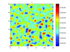
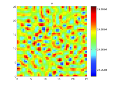
Figure 1: Simulation of the system 1.1 for the two-dimensional case $\Omega=[0,25]\times[0,25]$ with $\gamma=15$, $\beta=1.5$, $\rho=13$, $\alpha=7$, $a=103$, $b=77$, $k=0.125.$ The two figures show the $u$-component at $T=90$ and $T=150$ of a solution starting at a random perturbation near the stationary solution, where color represents the concentration of the activator.

References

- [1] Cahn, J. W., Hilliard, J. E., Free energy of a nonuniform system I. Interfacial free energy, J. Chem. Phys. 28 (1958) 258–267.
- [2] Garvie, M. R., Finite difference schemes for reaction-diffusion equations modeling predator-prey interactions in MATLAB, Bull. Math. Biol. 69 (2007) 931–956.
- [3] Gierer, A., Meinhardt, H., A theory of biological pattern formation, Kybernetik 12 (1972) 30–39.
- [4] Jiang, H., Global existence of solutions of an activator-inhibitor system, Discrete Contin. Dyn. Syst. 14 (2006) 737–751.
- [5] Li, M. D., Chen, S.H., Qin, Y. C., Boundedness and blow up for the general activator-inhibitor model, Acta Math. Appl. Sinica 11 (1995) 59–68.
- [6] Masuda, K., Takahashi, K., Reaction-diffusion systems in the Gierer-Meinhardt theory of biological pattern formation, Japan J. Appl. Math. 4 (1987) 47–58.
- [7] Meinhardt, H., Models of Biological Pattern Formation, Academic Press, 1982.
- [8] Murray, J. D., A pre-pattern formation mechanism for animal coat markings, J. Theor. Biol. 88 (1981) 161–199.
- [9] Murray, J. D., Mathematical Biology II: Spatial Models and Biomedical Applications, 3nd Edition, Springer-Verlag, New York, 2003.
- [10] Rothe, F., Global Solutions of Reaction-Diffusion Systems, Lecture notes in Math. 1072, Springer-Verlag, 1984.
- [11] Sander, E., Wanner, T., Pattern formation in a nonlinear model for animal coats, J. Differential Equations 191 (2003) 143–174.
- [12] Thomas, D., Artificial enzyme membranes, transport, memory, and oscillatory phenomena, in: D. Thomas, J.P. Kernevez (Eds.), Analysis and Control of Immobilized Enzyme Systems, Springer, Berlin, 1975, 115–150.
- [13] Triebel, H., Interpolation Theory, Function Spaces, Differential Operators, North-Holland, 1978.
- [14] Yagi, A., Abstract parabolic evolution equations and their applications, Springer, Berlin, 2010.