Wormholes with fluid sources: A no-go theorem and new examples

K. A. Bronnikov^a,b,c,1, K.A. Baleevskikh^b,2, and M.V. Skvortsova^d,3

^a

Center of Gravitation and Fundamental Metrology, VNIIMS, Ozyornaya St. 46, Moscow 119361, Russia

^b

Institute of Gravitation and Cosmology, Peoples’ Friendship University of Russia (RUDN University), Miklukho-Maklaya St. 6, Moscow 117198, Russia

^c

National Research Nuclear University MEPhI (Moscow Engineering Physics Institute), Kashirskoe highway 31, Moscow, 115409, Russia

^d

Peoples’ Friendship University of Russia (RUDN University), Miklukho-Maklaya St. 6, Moscow 117198, Russia

For static, spherically symmetric space-times in general relativity (GR), a no-go theorem is proved: it excludes the existence of wormholes with flat and/or AdS asymptotic regions on both sides of the throat if the source matter is isotropic, i.e., the radial and tangential pressures coincide. It explains why in all previous attempts to build such solutions it was necessary to introduce boundaries with thin shells that manifestly violate the isotropy of matter. Under a simple assumption on the behavior of the spherical radius $r(x)$, we obtain a number of examples of wormholes with isotropic matter and one or both de Sitter asymptotic regions, allowed by the no-go theorem. We also obtain twice asymptotically flat wormholes with anisotropic matter, both symmetric and asymmetric with respect to the throat, under the assumption that the scalar curvature is zero. These solutions may be on equal grounds interpreted as those of GR with a traceless stress-energy tensor and as vacuum solutions in a brane world. For such wormholes, the traversability conditions and gravitational lensing properties are briefly discussed. As a by-product, we obtain twice asymptotically flat regular black hole solutions with up to four Killing horizons. As another by-product, we point out intersection points in families of integral curves for the function $A(x)=g_{tt}$, parametrized by its values on the throat.

1 Introduction

Wormholes as two-way tunnels or shortcuts between different universes or different, otherwise distant regions of the same universe are at present a well-known and widely discussed subject, see, e.g., [1, 2, 3, 4, 5, 7, 6, 8]. Wormholes are of interest not only as a perspective “means of transportation” but also as possible time machines or accelerators [5, 7]. The simplest wormhole geometry is static, spherically symmetric, where the narrowest part, the throat, is simply a minimum of the spherical radius $r$. A majority of known exact wormhole solutions both in general relativity (GR) and alternative theories of gravity (e.g., [9, 10, 11, 13, 12]) are spherically symmetric.

In studies of macroscopic phenomena or possible artificial constructions, if our interest is in describing (potentially) realistic and manageable wormholes, there is a good reason to adhere to GR since it is this theory that is well verified by experiment at the macroscopic level and even serves as a tool in a number of engineering applications such as, for instance, global positioning systems. Then, the existence of traversable Lorentzian wormholes as solutions to the Einstein equations requires some kind of “exotic matter”, i.e., matter that violates the null energy condition (NEC) [5, 14], which is in turn a part of the weak energy condition (WEC) whose physical meaning is that the energy density is nonnegative in any reference frame.

Many spherically symmetric wormhole solutions in GR were first obtained with scalar field sources, beginning with a massless phantom scalar field [15, 16], and were later extended to include scalar field potentials as well as electromagnetic and other fields, see, e.g., [15, 17, 18, 19, 20, 21, 22] and references therein. Meanwhile, there appeared quite numerous examples of wormhole solutions with fluid sources with various equations of state or with unspecified matter whose stress-energy tensor (SET) components are formally called the density $\rho$ and pressure $p$, and the latter may be different in different directions — see, e.g, [13, 23, 24, 25, 26, 27, 28, 29]. An evident difficulty in this interpretation is that in such fluids in many cases (such as, for instance, $p=w\rho$ with $w<-1$) the velocity of sound calculated as $(dp/d\rho)^{1/2}$ turns out to be imaginary, which leads to a hydrodynamic instability with exponentially growing perturbations. A way out is to suppose that what we call a “fluid” actually consists of some fields with quite different perturbation dynamics.

These difficulties are absent (though others may appear) if, instead of standard GR, we adhere to the brane world concept. Let us recall that in brane world theories (see, e.g., the reviews [30, 31, 32] and references therein) the observable 4D world is a kind of domain wall in five or more dimensions of large or even infinite size. The standard-model fields are confined on the brane while gravity propagates in the surrounding bulk. The gravitational field on the brane itself can be described, at least in a large class of models related to Randall and Sundrum’s second model [33] (RS2), by modified 4D Einstein equations [34, 32], where, in addition to $T_{\mu\nu}$ — the SET of the 4D matter and a cosmological term $\Lambda_{4}g_{\mu\nu}$, there is also a tensor quadratic in $T_{\mu\nu}$, a contribution from bulk matter (if any), and a geometric term $E_{\mu\nu}$ representing a projection of the “electric” part of the 5D Weyl tensor onto the brane. In vacuum, when both 4D and 5D matter is absent, these equations take the form $G_{\mu\nu}+\Lambda_{4}g_{\mu\nu}=-E_{\mu\nu}$, where $G_{\mu\nu}$ is the 4D Einstein tensor. The tensor $E_{\mu\nu}$, connecting gravity on the brane with the bulk geometry, sometimes called the tidal SET, is traceless by construction. Due to its geometric origin, it is not subject to requirements like energy conditions or hydrodynamic stability. The form of $E_{\mu\nu}$, apart from its zero trace, is virtually arbitrary (as guaranteed by the known embedding theorems), so, if $\Lambda_{4}=0$ (a reasonable assumption for describing local objects), $R=0$ is the only unambiguous consequence of the equations $G_{\mu\nu}=-E_{\mu\nu}$.

A class of asymptotically flat wormhole solutions to the equation $R=0$ was obtained in [13], and it may be on equal grounds interpreted as describing vacuum gravitational fields in a brane world, existing due to a“tidal” influence from the fifth dimension, or GR wormholes supported by anisotropic fluids with a traceless SET. Other examples of solutions with $R=0$ appeared in [35, 36], their non-vacuum extensions in [37, 38, 39], in particular, with $\Lambda_{4}\neq 0$ in [39].

A common feature of these and many other wormhole solutions is that they were obtained using the spherical radius $r$ that has a minimum on the throat, as the radial coordinate, and, as a result, the solutions cover only one half of the wormhole space-time, the other half being its copy. Thus such wormholes are by construction ${\mathbb{Z}}_{2}$-symmetric with respect to their throats. Obtaining asymmetric wormholes using this coordinate is possible but technically rather inconvenient, see details in [13], and there are very few examples of such wormhole solutions [13, 35, 36, 22].

Another common feature of solutions with fluid sources is that the fluid is either anisotropic or, if isotropic, occupies a finite volume bounded by a junction surface, with a vacuum metric outside it. In most of the cases the junction surface is a thin shell with its own surface density and pressure. While such inclusions are often convenient for model construction, they look rather artificial, and it is worthwhile to consider matter distributions either directly adjoint to vacuum through a usual boundary, like a stellar surface, or gradually decaying and approaching vacuum at infinity.

In all cases, a vacuum geometry at infinity may be either flat, which is reasonable for describing a wormhole in the modern Universe, or (anti-) de Sitter ((A)dS), which is more suitable for possible wormholes in an inflationary universe or those related to vacuum bubbles (see, e.g., the recent paper [40] and references therein). One might claim that a static configuration with a dS asymptotic cannot be a wormhole because of inevitable existence of horizons; such horizons, however, are of cosmological rather than black hole nature, so it makes sense to widen the wormhole notion by admitting them. In an inflationary universe, such wormholes, connecting otherwise distant and causally disconnected regions of dS space, may in principle contribute to solving the horizon problem in cosmology, diminishing the necessary number of e-folds. Another application can be the modern accelerated Universe (or two such universes as possible locations of wormhole mouths) [41, 42, 43, 22, 44, 19, 45].

In this paper we will show that static, spherically symmetric, asymptotically flat or AdS wormhole geometries do not exist in GR with any kind of matter with isotropic pressure as a source (Section 2). On the contrary, asymptotically dS configurations are allowed, and we will construct examples of such wormhole solutions using the so-called quasiglobal coordinate $x$ [7, 46] such that $g_{tt}g_{xx}=-1$. The examples include both ${\mathbb{Z}}_{2}$-symmetric and asymmetric wormholes (Section 3). In Section 4 we present examples of symmetric and asymmetric asymptotically flat wormholes under the assumption $R=0$. We note that although the curvature coordinate $r$ is often favorable for obtaining analytic solutions (in [13] and [37] different wormhole and black hole solutions were obtained in an algorithmic form), the coordinate $x$ is more natural and transparent when dealing with black hole and wormhole geometries, even though our solutions in terms of $x$ are only numerical. As a by-product, in our study there emerge a number of regular, twice asymptotically flat black hole solutions with up to four Killing horizons. In Section 5 we consider the traversability properties of the twice asymptotically flat wormholes and calculate the light deflection angles in their geometries, leading to gravitational lensing. Section 6 contains some concluding remarks. Finally, in the Appendix we discuss an interesting property of the integral curves of our equations for the redshift function $A(x)=g_{tt}$: all curves beginning at the throat $x=0$ with the same slope $A^{\prime}$ but different values of $A(0)$, intersect at certain values of $x$. It turns out to be a manifestation of a general property of linear differential equations.

2 Basic equations. No-go theorem

2.1 General relations. The necessity of NEC violation

Let us begin with the general static, spherically symmetric metric which can be written in the form

$$ds^{2}={\,\rm e}^{2\gamma(u)}dt^{2}-{\,\rm e}^{2\alpha(u)}du^{2}-{\,\rm e}^{2\beta(u)}d\Omega^{2},$$ (1)

where $u$ is an arbitrary radial coordinate and $d\Omega^{2}=d\theta^{2}+\sin^{2}\theta d\varphi^{2}$ is the linear element on a unit sphere.

Then the Ricci tensor has the following nonzero components:

$${}R^{t}_{t}=-{\,\rm e}^{-2\alpha}[\gamma^{\prime\prime}+\gamma^{\prime}(\gamma^{\prime}-\alpha^{\prime}+2\beta^{\prime})],$$ (2)

$${}R^{u}_{u}=\!\!\ {-}{\,\rm e}^{-2\alpha}[\gamma^{\prime\prime}+2\beta^{\prime\prime}+\gamma^{\prime}{}^{2}+2\beta^{\prime}{}^{2}-\alpha^{\prime}(\gamma^{\prime}\!+\!2\beta^{\prime})],$$ (3)

$${}R^{\theta}_{\theta}=R^{\varphi}_{\varphi}={\,\rm e}^{-2\beta}-{\,\rm e}^{-2\alpha}[\beta^{\prime\prime}+\beta^{\prime}(\gamma^{\prime}-\alpha^{\prime}+2\beta^{\prime})],$$ (4)

where the prime stands for $d/du$. The Einstein equations can be written in two equivalent forms

$${}G_{\mu}^{\nu}\equiv R_{\mu}^{\nu}-{{\textstyle\frac{1}{2}}}\delta_{\mu}^{\nu}R=-T_{\mu}^{\nu},\qquad{\rm or}$$

$${}R_{\mu}^{\nu}=-(T_{\mu}^{\nu}-{{\textstyle\frac{1}{2}}}\delta_{\mu}^{\nu}T^{\alpha}_{\alpha}),$$ (5)

where $T_{\mu}^{\nu}$ is the stress-energy tensor (SET) of matter. The most general SET compatible with the geometry (1) has the form

$$T_{\mu}^{\nu}=\mathop{\rm diag}\nolimits(\rho,\ -p_{r},\ -p_{T},\ -p_{T}),$$ (6)

where $\rho$ is the energy density, $p_{r}$ is the radial pressure, and $p_{T}$ is the tangential pressure. These SET components may contain contributions of one or several physical fields of different spins and masses but can also be considered as hydrodynamic quantities, characterizing the density and pressures of one or several fluids. In this paper we consider $T_{\mu}^{\nu}$ as the SET either in a general form or as that of a single fluid, which is in general anisotropic ($p_{r}\not\equiv p_{T}$).

Let us illustrate the necessity of exotic matter for wormhole existence in space-times with the metric (1) taken as an example [5, 7]. Choosing the so-called quasiglobal coordinate $u=x$ under the condition $\alpha+\gamma=0$ and denoting ${\,\rm e}^{2\gamma}={\,\rm e}^{-2\alpha}=A(x)$, ${\,\rm e}^{\beta}=r(x)$, we rewrite the metric as

$$ds^{2}=A(x)dt^{2}-\frac{dx^{2}}{A(x)}-r^{2}(x)d\Omega^{2}.$$ (7)

A (traversable) wormhole geometry implies, by definition, that the function $r(x)$ has a regular minimum (say, at $x=x_{0}$), called a throat, and reaches values much larger than $r(x_{0})$ on both sides of the throat. It is also usually required that $A(x)>0$ in the whole range of $x$, which excludes horizons that characterize black hole rather than wormhole geometries. It may happen, however, that there is a horizon far away from the throat, for example, if the space-time is asymptotically de Sitter. If a wormhole connects two de Sitter universes or regions of a single de Sitter universe, it will have horizons on each side of the throat, but the latter lies in the region where $A(x)>0$.

The difference of the ${t\choose t}$ and ${x\choose x}$ components of the Einstein equations reads

$$2A\,r^{\prime\prime}/r=-(T^{t}_{t}-T^{x}_{x})\equiv-(\rho+p_{r}),$$ (8)

On the other hand, at a throat as a minimum of $r(x)$ we have

$$r>0,\qquad r^{\prime}=0,\qquad r^{\prime\prime}>0.$$ (9)

(In special cases where $r^{\prime\prime}=0$ at the minimum, it always holds $r^{\prime\prime}>0$ in its neighborhood.) Then from (8) it immediately follows $\rho+p_{r}<0$. This inequality does indeed look exotic, but to see an exact result, let us recall that the NEC requires $T_{\mu}^{\nu}k^{\mu}k_{\nu}\geq 0$, where $k^{\mu}$ is any null vector, $k^{\mu}k_{\mu}=0$. Choosing $k^{\mu}=(1/\sqrt{A},\sqrt{A},0,0)$, we see that $T_{\mu}^{\nu}k^{\mu}k_{\nu}=\rho+p_{r}$. Thus the inequality $\rho+p_{r}<0$ does indeed violate the NEC.

2.2 No-go theorem

There are three different nontrivial components in the Einstein equations for the metric (7), written using the quasiglobal gauge $\alpha+\gamma=0$:

$${}G^{t}_{t}=\frac{1}{r^{2}}[-1+A(2rr^{\prime\prime}+r^{\prime 2})+A^{\prime}rr^{\prime}]=-T^{t}_{t},$$ (10)

$${}G^{x}_{x}=\frac{1}{r^{2}}[-1+A^{\prime}rr^{\prime}+Ar^{\prime 2}]=-T^{x}_{x},$$ (11)

$${}G^{\theta}_{\theta}=G^{\phi}_{\phi}=\frac{1}{2r}[2Ar^{\prime\prime}+rA^{\prime\prime}+2A^{\prime}r^{\prime}]=p_{T},$$ (12)

where the prime again denotes $d/dx$, and (11) is the constraint equation, free from second-order derivatives. Note that $T^{t}_{t}$ is the energy density $\rho$ and $T^{x}_{x}=-p_{r}$ in a static (R-) region, where $A>0$, while beyond a horizon (if any), in a T-region where $A(x)<0$, where the metric describes a Kantowski-Sachs cosmology, $T^{x}_{x}$ is the energy density, and $-T^{t}_{t}$ is the pressure in the (spatial) $t$ direction.

It is of interest whether or not wormhole solutions can be obtained with a source in the form of an isotropic (Pascal) fluid, such that $p_{r}=p_{T}$. Let us show that the answer is negative if we require $A>0$ in the whole space.

If $p_{r}=p_{T}$, it follows $G^{x}_{x}=G^{\theta}_{\theta}$, and the difference of Eqs. (11) and (12) gives

$$r^{2}A^{\prime\prime}+2Arr^{\prime\prime}-2Ar^{\prime 2}+2=0.$$ (13)

The substitution $A(x)=D(x)/r^{2}(x)$ converts it to

$$D^{\prime\prime}-\frac{4D^{\prime}r^{\prime}}{r}+\frac{4Dr^{\prime 2}}{r^{2}}+2=0.$$ (14)

A possible minimum of $D(x)$ at some $x=x_{0}$ requires $D^{\prime}=0$ and $D^{\prime\prime}\geq 0$. Meanwhile, if $D^{\prime}=0$, Eq. (14) gives $D^{\prime\prime}\leq-2$, so that it is necessarily a maximum.

However, an asymptotically flat traversable wormhole requires $r\to\infty$ and $A\to 1$ as $x\to\pm\infty$, in an asymptotically anti-de Sitter wormhole it must be $A\sim r^{2}$ at large $r$, etc. In all such cases $D(x)\to\infty$ on both sides far from the throat, hence it should have a minimum, which, as we have seen, is impossible. We thus have the following theorem:

A static, spherically symmetric traversable wormhole with $r\to\infty$ and $A(x)r^{2}(x)\to\infty$ on both sides of the throat cannot be supported by any isotropic matter source with $p_{r}=p_{T}$.

This excludes, in particular, twice asymptotically flat and twice asymptotically AdS wormholes  as well as those asymptotically flat  on one end and AdS on the other. What is not excluded, is that one or both asymptotic regions are de Sitter: in this case, $r\to\infty$ but $A\sim-r^{2}$ at large $r$, and it is not necessary to have a minimum of $D(x)$.

The theorem has been proved using a specific coordinate condition but has an invariant meaning since the quantities $A=g_{tt}$ and $r^{2}=g_{\theta\theta}$ are insensitive to the choice of the radial coordinate. The existing wormhole solutions where an isotropic fluid occupies a finite region of space also do not contradict the theorem since they inevitably require “heavy” thin shells on the boundary between the fluid and vacuum regions [23, 24], and these shells are highly anisotropic in the sense that a tangential pressure is nonzero while the radial one is not defined (the radial direction is orthogonal to the shell).

3 Wormholes supported by
isotropic matter

3.1 Symmetric dS–dS wormholes

The opportunity of obtaining wormholes with two de Sitter asymptotics (dS–dS wormholes for short) supported by isotropic matter, allowed by the above no-go theorem, is of interest, in particular, because such wormholes may exist in an inflationary universe and provide causal connections between otherwise distant regions. We will construct examples of such solutions in this subsection.

Another opportunity of interest is a wormhole connecting de Sitter regions with different values of the cosmological constant, which may be interpreted as bubbles of true and false vacua. In such cases a wormhole can either play the role of a thick domain wall, or, on the contrary, directly connect regions separated by a domain wall. Such examples will be discussed in the next subsection.

Since there is no clear reason to assume any particular equation of state, we will instead specify the metric function $r(x)$ having a regular minimum at $x=0$ (the throat) and compatible with a de Sitter behavior of the metric at large $|x|$:

$$r(x)=\sqrt{a^{2}+x^{2}},\qquad a={\rm const}>0.$$ (15)

For a numerical study, we put $a=1$; remaining arbitrary, the parameter $a$ will then play the role of a length unit. Furthermore, assuming that the matter source is isotropic, $p_{r}=p_{T}$, we can use Eq. (13) for finding $A(x)$; after solving it, the metric will be known completely.

With (15) and $a=1$, Eq. (13) takes the form

$$(1+x^{2})^{2}A^{\prime\prime}+2(1-x^{2})A+2(1+x^{2})=0.$$ (16)

It is hard to solve this equation analytically, but its asymptotic form at large $|x|$, that is, $x^{2}A^{\prime\prime}-2A+2=0$, is easily integrated giving $A(x)=1+c_{1}x^{2}+c_{2}/x$ with $c_{1,2}={\rm const}$. Solutions with $c_{1}\geq 0$, corresponding to flat or AdS asymptotics, are excluded by the above no-go theorem, so the only possible asymptotic form of the metric is de Sitter, with $c_{1}<0$.

Examples of numerical solutions to Eq. (16) under the initial conditions $A(0)=A_{0}$, $A^{\prime}(0)=0$ are shown in Fig. 1 for $A_{0}=1,3,6,10,15$. It is of interest that all curves intersect at two symmetric points: $x\approx\pm 1.4109$, $A(x)\approx-1.4953$.

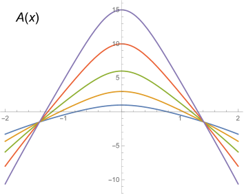
Figure 1: Solutions $A(x)$ of Eq. (16) for a symmetric dS–dS wormhole, corresponding to $A(0)=1,3,6,10,15$ (bottom-up along the ordinate axis) and $A^{\prime}(0)=0$.

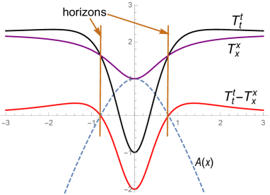
Figure 2: The metric function $A(x)$ and the SET components for a symmetric dS–dS wormhole described by the solution of Eq. (16) with $A(0)=1$ and $A^{\prime}(0)=0$.

The behavior of SET components in the wormhole model with $A(0)=1$ and $A^{\prime}(0)=0$, found from Eqs. (10) and (11), is shown in Fig. 2. The wormhole is ${\mathbb{Z}}_{2}$-symmetric relative to its throat ($x=0$), so all these functions are even. The values of the effective cosmological constant $\Lambda$ at large $|x|$ correspond to $A(x)\approx-\Lambda x^{2}/3$, thus it is clear from Fig. 1 that $\Lambda$ is the same at the two infinities but different for different values of $A(0)$. Its precise value is in each case determined as the common limit of $T^{t}_{t}$ and $T^{x}_{x}$, as exemplified by Fig. 2.

Note that the usual relations $T^{t}_{t}=\rho$ and $T^{x}_{x}=-p$ hold only in the static region, where $A(x)>0$. In a region where $A(x)<0$ (T-region), the coordinate $t$ is spatial, hence $-T^{t}_{t}=p_{t}$ is the pressure along the $t$ direction, while the density is $\rho=T^{x}_{x}$ since $x$ is now a temporal coordinate; however, the condition $r^{\prime\prime}>0$ in Eq. (8) (which is the same for any sign of $A$) leads to $\rho+p_{t}<0$, again violating the NEC. That $T^{t}_{t}$ and $T^{x}_{x}$ tend to the same constant value at large $x$ agrees with the de Sitter asymptotic behavior of the metric since the SET structure approaches that of a cosmological term, $T_{\mu}^{\nu}=\Lambda\delta_{\mu}^{\nu}$. One can also notice that this structure takes place on the horizon. Furthermore, in the whole space-time we have $T^{x}_{x}=T^{\theta}_{\theta}=-p_{T}$, but the fluid is anisotropic in the T-region since $p_{t}=-T^{t}_{t}\neq p_{T}$.

Fig. 3 shows the Carter-Penrose diagram of dS-dS wormholes, the same as presented in [41, 45], and potentially infinite both to the left and to the right: however, mutually isometric surfaces may be identified, such as, e.g., those depicted by lines AA’ and BB’ in Fig. 3, which means that the wormhole connects regions of the same de Sitter universe.

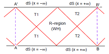
Figure 3: Carter-Penrose diagram showing the global structure of dS-dS wormholes. The regions labeled T1 correspond to the range $x<x_{-}$, those labeled T2 to the range $x>x_{+}$, where $x_{-}<x_{+}$ are the horizons (and $x_{-}=-x_{+}$ in a symmetric solution only).

3.2 Asymmetric configurations: dS–dS wormholes and black universes

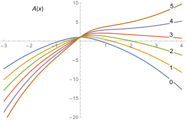
Figure 4: The function $A(x)$ for $A(0)=1$ and $A^{\prime}(0)=0,1,2,3,4,5$ (the latter values are written on the corresponding curves).

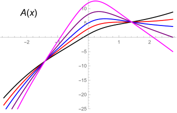
Figure 5: The function $A(x)$ for the same slope at the throat, $A^{\prime}(0)=6$ and $A(0)=1,3,5,8,12$ (bottom-up along the ordinate axis and conversely at large $|x|$)

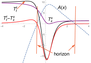
Figure 6: The function $A(x)$ and the SET components for the solution with $A(0)=8$ and $A^{\prime}(0)=6$, having two de Sitter asymptotics.with different curvature values.

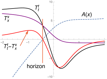
Figure 7: The same as in Fig. 6 but $A(0)=3$ and $A^{\prime}(0)=6$, with AdS behavior at large positive $x$.

Solutions to the same equation (16) with $A^{\prime}(0)\neq 0$ can also be obtained numerically. Some examples of such solutions are shown in Fig. 4 for $A(0)=0$ and $A^{\prime}(0)=0,1,2,3,4,5$. These plots show that at small values of $A^{\prime}(0)$ we obtain dS-dS wormholes with different values of $\Lambda$ at large positive and negative $x$. Such wormholes might connect space-time regions with different vacuum energy densities, for instant, a bubble of false vacuum with a region of true vacuum. The global structure diagram for all such space-times is the same as for symmetric dS-dS wormholes.

Larger values of $A^{\prime}(0)$ lead to configurations with a single horizon and an AdS asymptotic behavior as $x\to\infty$. There is an intermediate case with asymptotic flatness at large positive $x$, as is proved by the existence of solutions to Eq. (16) under the condition, e.g., $A(+\infty)=1$. All such configurations have the structure of black universes [47, 48, 17, 20], i.e., black holes in which beyond the horizon there is, instead of a singularity, an expanding universe tending to a de Sitter behavior at late times.

Figure 5 shows how the behavior of $A(x)$ changes if one keeps invariable the derivative $A^{\prime}(0)$ and changes $A(0)$. Again there are different asymptotic behaviors as $x\to+\infty$ depending on the value of $A(0)$. But again, just as in Fig. 1, all plots of $A(x)$ intersect at two points. More than that, these intersections occur at the same values of $x\approx\pm 1.4109$ as it happened for symmetric models, though the corresponding values of $A(x)$ are certainly different. All this cannot happen by chance, and indeed, one can prove that it is a manifestation of a general property of second-order linear differential equations, see the Appendix.

The SET components behave accordingly. Figs. 6 and 7 show their properties for two different cases, one for a dS-dS wormhole with different dS curvatures at two ends (Fig. 6), and the other where the right end is AdS. The corresponding values of the effective cosmological constant are the same as those of the SET components since at large $|x|$ all of them coincide (recall that we are here dealing with isotropic matter, hence $T^{x}_{x}=T^{\theta}_{\theta}=T^{\varphi}_{\varphi}$).

4 Asymptotically flat (M–M) wormholes and regular black holes

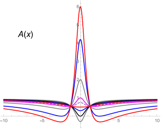
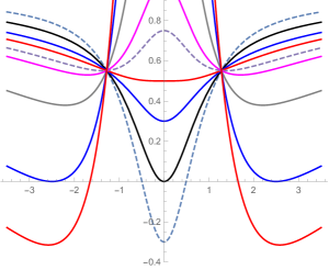
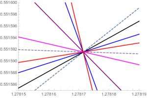
Figure 8: Symmetric solutions to Eq. (18) with $A^{\prime}(0)=0$ and $A(0)=-0.3,\ 0,\ 0.3,0.5,\ 0.75,\ 1,\ 2,\ 4.205,\ 6$ (bottom-up along the ordinate axis, and conversely at large $|x|$). Left — a general picture, middle — its part of interest enlarged. right — a neighborhood of the plots’ intersection point “under a microscope”.

Now let us abandon the source isotropy assumption and try to obtain some new models of twice asymptotically flat wormhole geometries. Since, as before, there is no clear reason to assume a particular form of the equations of state (which are now different for $p_{r}$ and $p_{T}$), let us, instead, again choose the function $r(x)$ in the form (15). In addition, let us assume a zero scalar curvature $R$ throughout the space. In this way we not only replace postulating another equation of state of the source matter, but also make it possible to interpret the results as vacuum solutions in an RS2-like brane world, somewhat similar to those found in [13], where some examples of ${\mathbb{Z}}_{2}$-symmetric wormhole solutions were obtained in an analytic form using the spherical radius $r$ as a coordinate. Now we will use the coordinate $x$ which is better for finding $Z_{2}$-asymmetric solutions, although these solutions will be only numerical.

For the metric (7) we have

$$R=\frac{2}{r^{2}}-A^{\prime\prime}-4A^{\prime}\frac{r^{\prime}}{r}-4A\frac{r^{\prime\prime}}{r}-2A\frac{r^{\prime 2}}{r^{2}}.$$ (17)

Therefore, under the assumption (15) for $r(x)$, with, as before $a=1$, the equation $R=0$ takes the form

$$A^{\prime\prime}+\frac{4x}{1+x^{2}}A^{\prime}+\frac{2(2+x^{2})}{(1+x^{2})^{2}}A=\frac{2}{1+x^{2}}.$$ (18)

At large $|x|$ the asymptotic form of this equation has the general solution $A=1+C_{1}/x+C_{2}/x^{2}$, $C_{1,2}={\rm const}$, which evidently corresponds to asymptotic flatness with a Schwarzschild-like metric. So, let us solve Eq. (18) under the initial conditions specified at $x=0$: $A(0)$ and $A^{\prime}(0)$, so that $A^{\prime}(0)=0$ should lead to an even function $A(x)$, hence a symmetric solution, and $A^{\prime}(0)\neq 0$ to an asymmetric one.

Examples of symmetric solutions to Eq. (18) with different $A(0)$ and $A^{\prime}(0)=0$ are plotted in Fig. 8. It is observed that at $0<A(0)=0.5$ we have wormholes with a minimum of $A(x)$ at the throat $x=0$, which is thus attracting for test particles. At larger $A(0)$ there appear two minima of $A(x)$ around the throat, acting as potential wells for test particles. A further increase of $A(0)$ makes these minima first equal to zero (at $A(0)\approx 4.205$) and then negative at still larger $A(0)$. We thus obtain regular black holes with either two double horizons or four simple horizons. A phenomenon of interest, as in Section 3, is that $A(\pm 1.278172)\approx 0.551892$ independently of $A(0)$, which is observed as the existence of two intersection points of all plots in Fig. 8. On the other hand, the initial values $A(0)=0$ and $A(0)<0$ lead to solutions with one double or two simple horizons, respectively, similar to those found in [37]. Thus we are again dealing with regular black holes instead of wormholes.

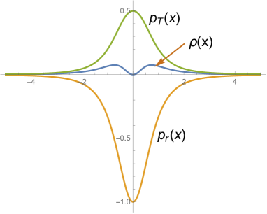
Figure 9: The density $\rho(x)$ and the pressures $p_{r}(x)$ and $p_{T}(x)$ for a symmetric wormhole with $A(0)=0.5$ and $A^{\prime}(0)=0$.

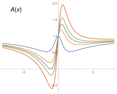
Figure 10: Solutions to Eq. (18) with $A(0)=1$ and $A^{\prime}(0)=0,1,1.5,2,3$ (upside-down for $x<0$ and bottom-up for $x>0$).

The effective matter density and pressures for an example of a symmetric wormhole model with $A(0)=0.5$ and $A^{\prime}(0)=0$ are shown in Fig. 9. The NEC violation at all $x$ is evident since $\rho+p_{r}<0$.

The above pictures are weakly or strongly deformed if we specify $A^{\prime}(0)\neq 0$. Let us consider some examples.

The behavior of $A(x)$ in the case $A(0)=1$ is depicted in Fig. 10. One sees that small nonzero values of $A^{\prime}(0)$ make the wormhole asymmetric without changing its global structure, but at $A^{\prime}(0)\approx 1.5$ emerges a double horizon which turns into a pair of simple horizons at larger $A^{\prime}(0)$. A similar behavior of the solutions is observed for all $A(0)\lesssim 4.2$, at which the corresponding symmetric solutions have no zeros and describe wormholes.

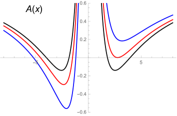
Figure 11: Solutions to Eq. (18) with $A(0)=5$ and $A^{\prime}(0)=0,0.8,2$ (upside-down for $x<0$ and bottom-up for $x>0$). The peaks near $x=0$ are similar to those in Fig. 8.

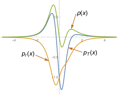
Figure 12: The density $\rho(x)$ and the pressures $p_{r}(x)$ and $p_{T}(x)$ for an asymmetric wormhole with $A(0)=1$ and $A^{\prime}(0)=1$.

At larger values of $A(0)$, at which even functions $A(x)$ have zeros shown in Fig. 8 (they describe symmetric regular black holes), the corresponding asymmetric space-times are also regular black holes, with the number of horizons from two to four, as is evident from Fig. 11, showing $A(x)$ with $A(0)=5$ and different $A^{\prime}(0)$.

Fig. 12 presents an example of the behavior of the effective density and pressures in an asymmetric wormhole model.

5 Wormhole traversability and lensing

In this section we will briefly discuss some important properties of asymptotically flat wormholes taking as examples some of the ${\mathbb{Z}}_{2}$-symmetric solutions for which the redshift function $A(x)$ is plotted in Fig. 8. The corresponding numerical estimates will evidently be true by order of magnitude for other typical solutions.

5.1 Traversability

Not all wormholes traversable by definition may really be used by a human being, or are “traversable in practice” [4]. A natural criterion for such traversability is that tidal accelerations due to inhomogeneity of the gravitational field should not exceed the Earth’s surface gravity, $g_{\oplus}\approx 9.8\,{\rm m/s^{2}}$. For a body moving in the radial direction, the tidal accelerations in a static, spherically symmetric metric can be described by Eqs. (13.4) and (13.6) from [4], which can be rewritten as follows in the notations of the metric (7):

$${}\Delta a_{\|}=R^{tx}_{\ \ tx}\Delta\xi_{\|}={{\displaystyle\frac{1}{2}}}A^{\prime\prime}\Delta\xi_{\|},$$ (19)

$${}\Delta a_{\bot}=\overline{\gamma}{}^{2}(R^{t\theta}_{\ \ t\theta}-\overline{\beta}{}^{2}R^{x\theta}_{\ \ x\theta}\Delta\xi_{\bot})$$

$${}\qquad=\overline{\gamma}{}^{2}\biggl{[}-{{\displaystyle\frac{1}{2}}}\frac{A^{\prime}r^{\prime}}{r}+\overline{\beta}{}^{2}\biggl{(}\frac{Ar^{\prime\prime}}{r}+{{\displaystyle\frac{1}{2}}}\frac{A^{\prime}r^{\prime}}{r}\biggr{)}\biggr{]}\Delta\xi_{\bot},$$ (20)

where $\Delta a$ are the tidal accelerations in the radial (_∥) and transveral (_⊥) directions, and $\Delta\xi$ are small displacements in the same directions. Furthermore, $\overline{\beta}{}=v/c$ is the velocity (in units of the speed of light) relative to the static reference frame, and $\overline{\gamma}{}=(1-\overline{\beta}{}^{2})^{-1/2}$ is the corresponding Lorentz factor. The expression (5.1) is especially simple for the throat $x=0$: since $r^{\prime}(0)=0$, it follows

$$\Delta a_{\bot}=\overline{\beta}{}^{2}\overline{\gamma}{}^{2}\frac{Ar^{\prime\prime}}{r}\Delta\xi_{\bot}.$$ (21)

In numerical estimates, the dimensionless quantities involved ($A,A^{\prime\prime},r,r^{\prime\prime},\overline{\beta}{},\overline{\gamma}{}$) are of the order of unity provided that $a=1$. Indeed, by (15), at the throat $x=0$ we have $r=1$ and $r^{\prime\prime}=1$, and by (18) $A^{\prime\prime}(0)=2-4A(0)$, the initial data for $A$ and $A^{\prime}$ are taken to be of the order of unity, and the values of all relevant quantities at $x\neq 0$ are of the same order as at $x=0$ or smaller.

However, our unit length is the arbitrary length $a$ equal to the throat radius, hence to obtain estimates in meters, each $d/dx$ should be divided by $a$ expressed in meters. We should also take into account that in the units where $c=1$ a second equals $3\mbox{$\cdot 10^{8}$}$ m, therefore $g_{\oplus}=9.8\,{\rm m/s^{2}}\approx 1.1\mbox{$\cdot 10^{-16}$}\,{\rm m}^{-1}$. So, assuming $\Delta\xi_{\|,\bot}=2$ m in Eqs. (19)–(21), from the requirement $|\Delta a_{\|,\bot}|\lesssim g_{\oplus}$ we obtain

$$a\gtrsim 10^{8}\ {\rm m}=10^{5}\ {\rm km},$$ (22)

that is, the throat radius must be larger than roughly eight Earth’s diameters. One can notice that the estimated tidal accelerations at a wormhole throat are of the same order of magnitude as tidal accelerations at a Schwarzschild horizon of the same radius (see, e.g., Eqs. (13.17) and (13.18) in [4]).

Another requirement is that a traveler should not experience too large center-of-mass accelerations. However, if the spacecraft moves along a geodesic, such an acceleration is zero (the usual free-fall weightlessness), and if not, everything depends of the engine activity.

5.2 Gravitational lensing

To calculate gravitational lensing as one of the most important potentially observable effects of wormholes, one can use the general formulas for asymptotically flat static, spherically symmetric space-times [49] (see, e.g., [50] for more recent references with calculations of light bending in various wormhole models). In our notations, the deflection angle $\alpha$, found by considering null geodesics in the metric (7), is given by

$${}\alpha=\alpha(x_{0})=I(x_{0})-\pi,$$

$${}I(x_{0})=2\int_{x_{0}}^{\infty}\frac{dx}{r(x)\sqrt{r^{2}(x)/b^{2}-A(x)}},$$ (23)

where $b=L/E$ is the so-called impact parameter charactering a particular null geodesic with the conserved energy parameter $E=A(x)dt/d\sigma$ and the conserved angular momentum $L=d\varphi/d\sigma$, $\sigma$ being an affine parameter along the geodesic. The coordinate value $x_{0}$ corresponds to the nearest approach of the photon path to the throat and is found from the condition $dr/d\sigma=0$ which leads to

$$A(x_{0})b^{2}=r^{2}(x_{0}).$$ (24)

It is clear that if ${\cal R}:=r(x_{0})>1$, then the photon is scattered against the wormhole, while the equality ${\cal R}=1$ tells us that the photon reaches the throat and then passes through the wormhole. We will restrict our calculations to photon paths with ${\cal R}>1$, mentioning that paths traversing a wormhole and images of another universe thus observed were considered in [51, 52]. Let us select for consideration three particular ${\mathbb{Z}}_{2}$-symmetric models from those depicted in Fig. 8, namely, one with $A(0)=1/3$ (in which $A(x)$ has a minimum on the throat), another with $A(0)=1$ (in which $A(x)$ is slightly peaked at the throat such that $A(0)=A(\infty)$), and the third one with $A(0)=3$ with a larger peak of $A(0)$ at the throat. A numerical calculation leads to the results shown in Fig. 13, covering a range of $x$ from a close vicinity of the throat to those where the deflection angles actually begin to follow the asymptotic law according to Einstein’s formula

$$\alpha({\cal R})\approx 4m/{\cal R},$$ (25)

where $m$ is the Schwarzschild mass that characterizes the almost Newtonian gravitational field at large $x$. As before, the scale along the horizontal axis corresponds to $a=1$, that is, the radius $r(x)$ is shown in units of the throat radius. Thus we compare light deflection near different wormholes with the same throat radius. These wormholes have different Schwarzschild masses $m(A(0))$:

$$m(0.3)\approx 0.89,\quad m(1)\approx 1.17,\quad m(3)\approx 2.09$$ (26)

(recall that these are “geometrized” masses with the dimension of length, $m=GM$, $G$ being the Newtonian gravitational constant and $M$ the conventional mass). For comparison, we also show the deflection angles for an Ellis wormhole [15, 16] with the same throat radius, described by the metric (7) with $r^{2}=1+x^{2}$ and $A(x)\equiv 1$ (its lensing properties were analyzed in detail in, e.g., [53, 54]), and for a Schwarzschild black hole with the same horizon radius, $2m=1$ (see detailed descriptions of Schwarzschild black hole lensing in, e.g., [55, 56, 57]).

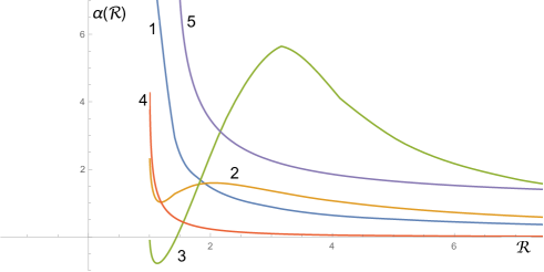
Figure 13: Light bending angles $\alpha$ as functions of the closest approach radius ${\cal R}$ for different wormholes and a Schwarzschild black hole. Curves 1–3 show $\alpha({\cal R})$ for wormholes with the throat radius $a=1$ and $A(0)=1/3,1,3$, respectively, curve 4 for an Ellis wormhole with the same throat radius, and curve 5 for a Schwarzschild black hole with the same radius, $2m=1$, of the event horizon.

As is clear from the figure, the wormhole lensing properties substantially depend on the profile of $A(x)$: curve 1, corresponding to $A(0)=0.3$ such that $A(x)$ has a minimum at the throat, is rather similar to curve 5 describing Schwarzschild black hole lensing, the main difference being that in the Schwarzschild case $\alpha\to\infty$ as ${\cal R}\to 3/2$ (a logarithmic divergence at the so-called photon sphere), while the same happens only as ${\cal R}\to 1$ for wormholes. Curve 2 shows a decrease in $\alpha$ in the region where $A(x)$ is decreasing. Actually, the role of $A(x)$ is similar to that of the Newtonian gravitational potential in classical physics, so where $A^{\prime}<0$, the gravitational field is repulsive for both massive particles and photons. This effect is still stronger if the peak of $A(x)$ is larger and can even lead to negative light bending at some ${\cal R}$ as can be seen for curve 3. Curve 4 pertains to the Ellis wormhole, which is massless and therefore much weaker affects the light beams, and its $\alpha({\cal R})$ quicker decays at large ${\cal R}$; however, $\alpha({\cal R})$ also diverges near ${\cal R}=1$.

6 Concluding remarks

Let us enumerate the main results of this study:

1. We have proved a no-go theorem showing that it is impossible to obtain static asymptotically flat or AdS wormholes without horizons, supported by isotropic matter. It explains why in all previous attempts to build such solutions it was necessary to introduce boundaries with thin shells.

2. We have obtained a family of wormholes with isotropic matter which connect two de Sitter worlds with the same or different curvature. In the symmetric case, such “bridges” may connect distant regions of the same inflationary universe making them causally connected. It is of interest that, unlike other models where the wormhole throat expands together with the universes it connects, in our solutions the throat radius is constant.

3. It is important that even though we introduced, as sources of gravity, isotropic fluids in the static space-time region, these fluids inevitably become anisotropic in a T-region with a time-dependent Kantowski-Sachs type metric.

4. We have obtained a number of new numerical asymptotically flat solutions to the equation $R=0$, describing ${\mathbb{Z}}_{2}$-symmetric or asymmetric wormhole and regular black hole configurations, among which asymmetric ones are obtained quite naturally by specifying asymmetric initial data at $x=0$. Some asymptotically flat metrics with $R=0$ contain up to four Killing horizons.

5. We have shown that the traversability condition for wormholes considered here in terms of sufficiently low tidal forces are actually the same as in other models and require a throat radius of about $10^{5}$ km or more. A brief consideration of the lensing properties of our twice asymptotically flat wormholes have revealed their distinguishing features, but a more complete analysis of this important phenomenon is postponed for future studies.

6. While solving the equations with respect to $A(x)=g_{tt}$, expressing the isotropy condition $p_{r}=p_{T}$ in Section 3, or zero scalar curvature in Section 4, we have revealed intersection points in families of integral curves, corresponding to different initial values of $A$ but the same initial slope $A^{\prime}$. It is a manifestation of a general interesting property of linear ordinary differential equations, discussed in the Appendix. For the integral curves of $A(x)$, the existence of such intersections leads to the following general rule: given a fixed initial slope $A^{\prime}(0)$, a curve that begins higher at $x=0$ (that is, $A(0)$ is larger), ends lower at large $|x|$ in both positive and negative directions.

Our results have been obtained in terms of the quasiglobal coordinate $x$. Let us comment on some other choices of the radial coordinate which seem to be more intuitively understandable. One of them is the curvature, or Schwarzschild coordinate, $r$, equal to the spherical radius ${\,\rm e}^{\beta}$ in the metric (1). As already explained in the introduction, this choice is not good if $r$ has a minimum, in particular, in all wormhole space-times. We can easily transform our solutions to $r$ as a new coordinate by the substitution $x=\pm\sqrt{r^{2}-1}$, which will result in two separate branches for positive and negative $x$ in each solution. These branches will be identical when obtained from ${\mathbb{Z}}_{2}$-symmetric solutions, but in asymmetric (that is, more general) ones the unity of two branches will become quite non-obvious. However, $r$ is a convenient parameter for showing the wormhole lensing properties and their comparison with lensing by a Schwarzschild black hole, see Fig. 13.

Another popular choice is the Gaussian, or proper radial distance coordinate $l$, such that ${\,\rm e}^{\alpha}\equiv 0$ in (1). This coordinate is quite suitable for describing wormhole space-times but is not good enough for black holes since at an extremal (double) horizon, where, in terms of our metric (7), $A(x)\sim(x-x_{\rm hor})^{2}$, the proper radial distance diverges. So, if we used the coordinate $l$ for finding the solutions, we would lose their natural sequence at transitions from wormhole to black hole cases, and we would simply lose the solution with $A(0)=0$, see Fig. 8.

In a flat asymptotic region all three coordinates coincide, and at an (A)dS infinity the Schwarzschild ($r$) and quasiglobal ($x$) coordinates also coincide. However, in a strong field region, as we see, the coordinate $x$ is the most preferable. It is always admissible at wormhole throats, while at horizons in static, spherically symmetric space-times it is always finite and behaves, up to a nonzero constant factor, like a Kruskal-like coordinate needed to cross the horizon [7]; it can therefore be used to jointly describe inner and outer regions of black holes (hence the name “quasiglobal”). Apart from the fact that, in our notations, $r\equiv x$ in the Schwarzschild-(A)dS solutions and their charged counterparts, the coordinate $x$ is widely used in solutions with scalar fields, see, e.g., [10, 17, 47, 58, 59] and many others.

It should be noted that such physically meaningful quantities as $A(x)\equiv g_{tt}$ and the nonzero SET components $T_{\mu}^{\nu}$ in the metric (1) (the density and pressures) are insensitive to the choice of a radial coordinate and behave as scalars at its transformations. Therefore in cases where two coordinates are equally admissible, such as $x$ and $l$ in asymptotically flat wormholes, a transition from one such coordinate to another will merely result in non-uniform but finite stretching or squeezing of the corresponding plots along the horizontal axis.

Appendix

In this Appendix we prove and discuss a very simple and interesting property of linear second-order ordinary differential equations (L2-ODE), which must have numerous applications and must probably be well known to mathematicians, but we were unable to find proper references.

Consider a general L2-ODE for $y(x)$:

$$A(x)y^{\prime\prime}+B(x)y^{\prime}+C(x)y=F(x),$$ (A.1)

where the prime means $d/dx$, and all quantities involved are supposed to be real. Let there be initial conditions at some $x_{0}$:

$$y(x_{0})=a,\qquad y^{\prime}(x_{0})=b.$$ (A.2)

The general solution to Eq. (A.1) is a function of $x$ and the initial data $a,b$. On the other hand,

$${}y=y(x,a,b)=C_{1}y_{1}(x)+C_{2}y_{2}(x)+y_{3}(x),$$

$${}C_{1},C_{2}={\rm const},$$ (A.3)

where $y_{1}(x)$ and $y_{2}(x)$ are two linearly independent solutions to the homogeneous equation (A.1), i.e., for $F(x)\equiv 0$, and $y_{3}(x)$ is a special solution to the inhomogeneous equation (A.1).

Suppose we know the functions $y_{i}(x)$. Then, comparing (A.2) and (Appendix), we can write for $x=x_{0}$

$${}C_{1}y_{10}+C_{2}y_{20}=a-y_{30},$$

$${}C_{1}y^{\prime}_{10}+C_{2}y^{\prime}_{20}=b-y^{\prime}_{30},$$ (A.4)

with the constants $y_{i0}=y_{i}(x_{0})$ and $y^{\prime}_{i0}=y^{\prime}_{i}(x_{0})$, $i=1,2,3$. The algebraic equations (Appendix) may be used to express the constants $C_{1,2}$ in terms of the initial data $a,b$. By Kramer’s formulas, we have ($i=1,2$)

$$C_{i}=\frac{W_{i}}{W_{0}},\qquad W_{0}=\begin{vmatrix}y_{10}&y_{20}\\ y^{\prime}_{10}&y^{\prime}_{20}\end{vmatrix},$$ (A.5)

where $W_{0}\neq 0$ is the Wronskian of $y_{1,2}$ at $x=x_{0}$, and $W_{i}$ are the determinants obtained from $W_{0}$ by replacing its $i$-th column with that of the r.h.s. of (Appendix). Thus we obtain

$${}C_{1}=W_{0}^{-1}[(a-y_{30})y^{\prime}_{20}-(b-y^{\prime}_{30})y_{20}],$$

$${}C_{2}=-W_{0}^{-1}[(a-y_{30})y^{\prime}_{10}-(b-y^{\prime}_{30})y_{10}],$$

Substituting this into (Appendix), we present the solution with explicit dependence on the initial data $a$ and $b$:

$${}y(x,a,b)=\frac{y_{1}(x)}{W_{0}}[(a-y_{30})y^{\prime}_{20}-(b-y^{\prime}_{30})y_{20}]$$

$${}-\frac{y_{2}(x)}{W_{0}}[(a-y_{30})y^{\prime}_{10}-(b-y^{\prime}_{30})y_{10}]+y_{3}(x).$$ (A.6)

Now we put the following question: Is there such a value of $x$, say, $x=x_{*}$, at which the function $y$ takes the same value for any choice of $a$ if $b$ is fixed? It will mean that all integral curves $y(x)$, beginning at $x_{0}$ with the same slope $y^{\prime}(x_{0})=b$ but different starting points $y(x_{0})=a$, intersect at $x=x_{*}$.

If such a value does exist, then at $x=x_{*}$ we should have $\partial y/\partial a=0$, where $y=y(x,a,b)$ is given by (Appendix). Explicitly, the condition $\partial y/\partial a=0$ has the form

$$y_{1}(x_{*})y^{\prime}_{20}=y_{2}(x_{*})y^{\prime}_{10}.$$ (A.7)

It is an algebraic (in general, transcendental) equation with respect to $x_{*}$ if the functions $y_{1,2}(x)$ are known. This equation may have any number of solutions, from zero to infinity. Anyway, it is clear that the existence of such intersection points is quite a general phenomenon.

Some important observations are in order:

1. It is easily verified that Eq. (A.7) is insensitive to a particular choice of two linearly independent solutions $y_{1,2}$ to the homogeneous equation (A.1).

2. The value of $x_{*}$ is insensitive to the inhomogeneity $F(x)$ in Eq. (A.1). It only depends on the left-hand side of (A.1) and on the choice of $x_{0}$.

3. The value of $x_{*}$ does not depend on $b$. In other words, different sets of integral curves beginning at $x=x_{0}$ at different “heights” $a$ but with the same slope $b$, intersect at the same $x=x_{*}$ for all values of $b$ (though at a $b$-dependent height).

Example. Consider the simplest L2-ODE

$$y^{\prime\prime}+Ky=L,\hskip 28.45274ptK,L={\rm const}.$$ (A.8)

Then, first of all, we can write the solution $y_{3}=L/K$ of the inhomogeneous equation, which has no effect on anything further on.

Next, if $K=k^{2}>0$, we can write

$$y_{1}(x)=\cos kx,\quad y_{2}(x)=\sin kx,$$ (A.9)

and if we choose $x_{0}=0$, then Eq. (A.7) gives $\cos kx_{*}=0\ \ \Rightarrow\ \ x_{*}=\pi/2+\pi n$, where $n\in{\mathbb{Z}}$, an infinite number of solutions, or an infinite number of intersection points of the integral curves along the $x$ axis. The same result is obtained if we take other $y_{1,2}$, for example, $y_{1,2}=\cos kx\pm\sin kx$.

If the initial data are specified at another $x_{0}$, the intersection points are located at other $x$. For example, if $x_{0}=\pi/(4k)$, then Eq. (A.7) gives $kx_{*}=-\pi/4+\pi n$, $n\in{\mathbb{Z}}$, again an infinite number of intersection points, but they are located at other $x_{*}$ than for $x_{0}=0$.

Lastly, if $K=-k^{2}<0$, then, instead of (A.9),

$${}y_{1}=e^{kx},\qquad y_{2}=e^{-kx},\quad{\rm or\ equivalently}$$

$${}y_{1}=\cosh kx,\qquad y_{2}=\sinh kx.$$ (A.10)

If we choose $x_{0}=0$, Eq. (A.7) leads to $\cosh kx_{*}=0$, so there is no solution. Thus the integral curves of Eq. (A.8) with $K<0$, beginning at $x_{0}=0$ with the same slope, do not intersect. The same result is obtained for any $x_{0}\neq 0$.

This example illustrates the observation that the number of intersection points of integral curves may vary from zero to infinity.

Acknowledgments

We thank Sergei Bolokhov for helpful discussions. The work of KB was partly performed within the framework of the Center FRPP supported by MEPhI Academic Excellence Project (contract No. 02.a03.21.0005, 27.08.2013). This publication was also supported by the Ministry of Education and Science of the Russian Federation (Agreement number 02.A03.21.0008) and by RFBR grant 16-02-00602.

References

- [1] L. Flamm, Beiträge zur Einsteinschen Gravitationstheorie. Phys. Z. 17, 48 (1916).
- [2] A. Einstein and N. Rosen, The particle problem in the general theory of relativity. Phys. Rev. 48, 73 (1935).
- [3] J.A. Wheeler, On the nature of quantum geometrodynamics. Ann. Phys. 2 (6), 604 (1957).
- [4] M. Visser, Lorentzian Wormholes: From Einstein to Hawking (American Institute of Physics, New York, 1995)
- [5] M.S. Morris and K.S. Thorne, Wormholes in spacetime and their use for interstellar travel: A tool for teaching general relativity. Am. J. Phys. 56, 395 (1988).
- [6] F.S.N. Lobo, Exotic solutions in General Relativity: Traversable wormholes and ?warp drive? spacetimes. In: Classical and Quantum Gravity Research, p. 1-78 (Nova Sci. Pub., 2008); ArXiv: 0710.4474.
- [7] K.A. Bronnikov and S.G. Rubin, Black Holes, Cosmology, and Extra Dimensions (World Scientific, 2012).
- [8] K.A. Bronnikov and M.V. Skvortsova, Wormholes leading to extra dimensions. Grav. Cosmol. 22, 316 (2016); arXiv: 1608,04974.
- [9] K.A. Bronnikov and A.M. Galiakhmetov, Wormholes without exotic matter in Einstein-Cartan theory. Grav. Cosmol. 21, 283 (2015); arXiv: 1508.01114.
- [10] K.A. Bronnikov and A.M. Galiakhmetov, Wormholes and black universes without phantom fields in Einstein-Cartan theory. Phys. Rev. D 94, 124006 (2016); arXiv: 1607.07791.
- [11] G. Dotti, J. Oliva, and R. Troncoso, Static wormhole solution for higher-dimensional gravity in vacuum. Phys. Rev. D 75, 024002 (2007); hep-th/0607062.
- [12] T. Harko, F.S.N. Lobo, M.K. Mak, and S.V. Sushkov, Gravitationally modified wormholes without exotic matter, Phys. Rev. D 87, 067504 (2013); arXiv: 1301.6878.
- [13] K.A. Bronnikov and S.-W. Kim, Possible wormholes in a brane world. Phys. Rev. D 67, 064027 (2003), gr-qc/0212112.
- [14] D. Hochberg and M. Visser, Geometric structure of the generic static traversable wormhole throat. Phys. Rev. D 56, 4745 (1997); gr-qc/9704082.
- [15] K.A. Bronnikov, Scalar-tensor theory and scalar charge. Acta Phys. Pol. B 4, 251 (1973).
- [16] H. Ellis, Ether flow through a drainhole — a particle model in general relativity. J. Math. Phys. 14, 104 (1973).
- [17] S.V. Bolokhov, K.A. Bronnikov, and M.V. Skvortsova, Magnetic black universes and wormholes with a phantom scalar. Class. Quantum Grav.29, 245006 (2012).
- [18] G. Clement, J.C. Fabris, and M.E. Rodrigues, Phantom black holes in Einstein-Maxwell-dilaton theory. Phys. Rev. D 79, 064021 (2009); arXiv: 0901.4543.
- [19] Andres Anabalon and Adolfo Cisterna, Asymptotically (anti) de Sitter black holes and wormholes with a self-interacting scalar field in four dimensions. Phys. Rev. D 85, 084035 (2012); arXiv: 1201.2008.
- [20] K.A. Bronnikov and P.A. Korolyov, Magnetic wormholes and black universes with invisible ghosts. Grav. Cosmol. 21, 157 (2015); arXiv: 1503.02956.
- [21] K.A. Bronnikov. Trapped ghosts as sources for wormholes and regular black holes. The stability problem. In: Wormholes, Warp Drives and Energy Conditions, ed. F.S.N. Lobo, Springer, 2017, p. 137-160.
- [22] A.B. Balakin, José P.S. Lemos, and A.E. Zayats, Nonminimal coupling for the gravitational and electromagnetic fields: Traversable electric wormholes. Phys. Rev. D 81, 084015 (2010).
- [23] S. Sushkov, Wormholes supported by a phantom energy. Phys. Rev. D 71, 043520 (2005); gr-qc/0502084.
- [24] F.S.N. Lobo, Phantom energy traversable wormholes. Phys. Rev. D 71, 084011 (2005); gr-qc/0502099.
- [25] F. Rahaman, M. Kalam, M. Sarker, and K. Gayen, A theoretical construction of wormhole supported by phantom energy. Phys. Lett. B 633, 161 (2006); gr-qc/0512075.
- [26] F. Parsaei, and N. Riazi, New asymptotically flat phantom wormhole solutions. Phys. Rev. D 87, 084030 (2013); arXiv: 1212.5806.
- [27] Francisco S. N. Lobo, Chaplygin traversable wormholes. Phys. Rev. D 73, 064028 (2006); gr-qc/0511003.
- [28] M. Cataldo, L. Liempi, and P. Rodriguez, Static spherically symmetric wormholes with isotropic pressure Phys. Lett. B 757, 130-135 (2016); arXiv: 1604.04578.
- [29] P.K.F. Kuhfittig, Conformal-symmetry wormholes supported by a perfect fluid. New Horizons in Mathematical Physics 1, 14 (2017); arXiv: 1707.04150.
- [30] V. A. Rubakov, Large and infinite extra dimensions. Usp. Fiz. Nauk 171, 913 (2001) [Phys. Usp. 44, 871 (2001)].
- [31] G. Gabadadze, Cargese lectures on brane induced gravity, Nucl. Phys. Proc. Suppl. 171, 88 (2007); arXiv: 0705.1929.
- [32] R. Maartens and K. Koyama, Brane-world gravity. Living Rev. Relativity 13, 5 (2010); arXiv: 1004.3962.
- [33] L. Randall and R. Sundrum, An alternative to compactification. Phys. Rev. Lett. 83, 4690 (1999).
- [34] T. Shiromizu, K. Maeda, and M. Sasaki, The Einstein equations on the 3-brane world. Phys. Rev. D 62, 024012 (2000).
- [35] N. Dadhich, S. Kar, S. Mukherjee, and M. Visser, spacetimes and self-dual Lorentzian wormholes. Phys. Rev. D 65, 064004 (2002); gr-qc/0109069.
- [36] A.G. Agnese and M.La Camera, Traceless stress-energy and traversable wormholes. Nuovo Cim. B 117, 647 (2002); gr-qc/0203067.
- [37] K.A. Bronnikov, V.N. Melnikov and H. Dehnen, General class of brane-world black holes. Phys. Rev. D 68, 024025 (2003).
- [38] F.S.N. Lobo, A general class of braneworld wormholes. Phys. Rev. D 75, 064027 (2007)’; gr-qc/0701133.
- [39] C. Molina, J. C. S. Neves, Wormholes in de Sitter branes. Phys. Rev. D 86, 024015 (2012); arXiv: 1204.1291.
- [40] E.F. Eiroa, G. Figueroa Aguirre, and J.M.M. Senovilla, Pure double-layer bubbles in quadratic F(R) gravity. Phys. Rev. D 95, 124021 (2017); arXiv: 1704.00698.
- [41] José P. S. Lemos, Francisco S. N. Lobo, Sergio Quinet de Oliveira, Morris-Thorne wormholes with a cosmological constant. Phys. Rev. D 68, 064004 (2003); gr-qc/0302049.
- [42] S.V. Sushkov and S.-W. Kim, Cosmological evolution of a ghost scalar field. Gen. Rel. Grav. 36, 1671 (2004); gr-qc/0404037
- [43] S.V. Sushkov and Yuan-Zhong Zhang, Scalar wormholes in cosmological setting and their instability. Phys. Rev. D 77, 024042 (2008); arXiv: 0712.1727.
- [44] C. Molina, P.Martin-Moruno, and P.F. González-Díaz, Isotropic extensions of the vacuum solutions in general relativity. Phys. Rev. D 84, 104013 (2011); arXiv: 1107.4627.
- [45] A. Mokeeva and V. Popov, Isotropization in Chaplygin matter universes connected by a wormhole. Int. J. Mod. Phys. D 22, 1350067 (2013); arXiv: 1304.5608.
- [46] K.A. Bronnikov, Spherically symmetric false vacuum: no-go theorems and global structure. Phys. Rev. D 64, 064013 (2001); gr-qc/0104092.
- [47] K.A. Bronnikov and J.C. Fabris, Regular phantom black holes. Phys. Rev. Lett. 96, 251101 (2006).
- [48] K.A. Bronnikov, V.N. Melnikov and H. Dehnen, Regular black holes and black universes. Gen. Rel. Grav. 39, 973 (2007).
- [49] V. Bozza, Gravitational lensing in the strong field limit, Phys. Rev. D 66, 103001 (2002).
- [50] Naoki Tsukamoto, Deflection angle in the strong deflection limit in a general asymptotically flat, static, spherically symmetric spacetime. Phys. Rev. D 95, 064035 (2017); arXiv: 1612.08251.
- [51] Alexander Shatskiy, Image of another universe being observed through a wormhole throat Phys. Usp. 52, 811 (2009); arXiv: 0809.0362.
- [52] A. Shatskiy, Yu.Yu. Kovalev, I.D. Novikov, Model predictions of the results of interferometric observations for stars under conditions of strong gravitational scattering by black holes and wormholes. JETP 120, 798 (2015); arXiv: 1607.03091.
- [53] F. Abe, Gravitational microlensing by the Ellis wormhole. Astroph. J. 725, 787-793 (2010); arXiv: 1009.6084
- [54] Naoki Tsukamoto, Strong deflection limit analysis and gravitational lensing of an Ellis wormhole. Phys. Rev. D 94, 124001 (2016); arXiv: 1607.07022
- [55] Charles Darwin, The gravity field of a particle. Proc. R. Soc. Lond. A 249, 180 (1959).
- [56] K. S. Virbhadra and G. F. R. Ellis, Schwarzschild black hole lensing. Phys. Rev. D 62, 084003 (2000); astro-ph/9904193.
- [57] G. S. Bisnovatyi-Kogan and O. Yu. Tsupko. Strong gravitational lensing by Schwarzschild black holes. Astrophysics 51 (1), 99 (2008); arXiv: 0803.2468.
- [58] J.A. Gonzalez, F.S. Guzman, O. Sarbach, Instability of wormholes supported by a ghost scalar field. I. Linear stability analysis. Class. Quantum Grav. 26, 015010 (2009); arXiv: 0806.0608.
- [59] K.A. Bronnikov and P.A. Korolyov. On wormholeas with long throats and the stability problem. Grav. Cosmol. 23 (3), 273 (2017); arXiv: 1705.05906.