Adaptive Lock-Free Data Structures in Haskell:
A General Method for Concurrent Implementation Swapping

Abstract.

A key part of implementing high-level languages is providing built-in and default data structures. Yet selecting good defaults is hard. A mutable data structure’s workload is not known in advance, and it may shift over its lifetime—e.g., between read-heavy and write-heavy, or from heavy contention by multiple threads to single-threaded or low-frequency use. One idea is to switch implementations adaptively, but it is nontrivial to switch the implementation of a concurrent data structure at runtime. Performing the transition requires a concurrent snapshot of data structure contents, which normally demands special engineering in the data structure’s design. However, in this paper we identify and formalize an relevant property of lock-free algorithms. Namely, lock-freedom is sufficient to guarantee that freezing memory locations in an arbitrary order will result in a valid snapshot.

Several functional languages have data structures that freeze and thaw, transitioning between mutable and immutable, such as Haskell vectors and Clojure transients, but these enable only single-threaded writers. We generalize this approach to augment an arbitrary lock-free data structure with the ability to gradually freeze and optionally transition to a new representation. This augmentation doesn’t require changing the algorithm or code for the data structure, only replacing its datatype for mutable references with a freezable variant. In this paper, we present an algorithm for lifting plain to adaptive data and prove that the resulting hybrid data structure is itself lock-free, linearizable, and simulates the original. We also perform an empirical case study in the context of heating up and cooling down concurrent maps.

1. Introduction

High-level, productivity languages are equipped with rich built-in data structures, such as mutable and immutable dictionaries. If we envision parallel-by-default languages of the future, programmers may expect that built-in data structures support concurrency too. This will require intelligent selections of default implementations to not incur undue overhead under either contended or single-threaded access patterns.

If you need a one-size-fits all choice, automatically selecting or swapping between data structure implementations at runtime has a natural appeal (Xu, 2013; Bolz et al., 2013). These swaps can match implementations to observed workloads: e.g., relative frequency of methods, degree of contention, or data structure contents. In the sequential case, adaptive data structures are already used to good effect by tracing JIT compilers for dynamic languages such as PyPy and Pycket (Bauman et al., 2015), which, for instance, optimistically assumes that an array of floats will continue to contain only floats, and fall back automatically to a more general representation only if this is violated.

But such adaptive data structures are much harder to achieve in concurrent settings than in sequential. While implementations of adaptive data structures exist in Java and other languages (Kusum et al., 2016; Xu, 2013; De Wael et al., 2015), no techniques exist to apply this form of adaptation in a multithreaded scenario. How can we convert a data structure that is being mutated concurrently? The problem is similar to that of concurrent garbage collection, where a collector tries to move an object graph while the mutator modifies it.

In this paper we introduce a general approach for freezing a concurrent, lock-free, mutable data structure—subject only to a few restrictions on the shape of methods and which instructions linearize. We do this using the simple notion of a freezable reference that replaces the regular mutable reference. Remarkably, it is possible to freeze the references within a data structure in an arbitrary order, and still have a valid snapshot. The snapshot is valid because all operations on the original structure are linearizable, which prevents intermediate modifications due to half-completed methods from corrupting the structure or affecting its logical contents.

Using freezable references, we show how to build a hybrid data structure that transitions between two lock-free representations, while in turn preserving lock-freedom and linearizability for the complete structure. The end result is a hybrid exposing a special method to trigger transition between representations, with user-exposed snapshotting being a special case of transitioning to an immutable data structure inside a reference that allows $O(1)$ exact snapshots.

The contributions of this paper are:

• We prove a property of lock-free data structures that has not previously been formalized: that the memory locations making up the structure can be frozen in arbitrary order, providing a valid snapshot state. We apply the tools of operational semantics in this concurrency proof, which enables more precision than is standard for such proofs.

• We present a novel algorithm for building hybrid, adaptive data structures which we prove is lock-free, linearizable, and correctly models the original structures (§ 6). Our formal model uses an abstract machine that models clients interacting with a lock free data structure.

• We demonstrate how to apply the method in a Haskell library that transitions between a concurrent Ctrie (Prokopec et al., 2012) and a purely functional hashmap (§ 7.1). We perform a case study measuring the benefit of transitioning from a concurrent data structure to a representation optimized for read-heavy workloads (§ 8).

2. Background and Related Work

At first glance, the problem we pose would seem to bear similarity to previous work on multi-word transactions (MCAS or STM). For instance, Harris et al. (2002) propose a way to perform multi-word CAS (MCAS). However this approach is effective only for small, fixed numbers of locations rather than large, lock-free data structures—it must create a descriptor proportional to all addresses being changed, which we cannot do for a data structure which grows during transitioning, and would be inefficient in any case. Software transactional memory (Herlihy et al., 2003b) can be used on dynamic-sized data to implement obstruction-free data structures (Herlihy et al., 2003a). However, STM’s optimistic approach in general cannot scale to large data structures.

Snapshots:

Further, Afek et al. (1993) give an algorithm to archive atomic snapshots of shared memory, however it again works for fixed locations and does not apply to dynamic data structures. Furthermore, snapshot alone cannot implement transition between lock-free data structures, building a new structure based on the snapshot would lose the effects of ongoing method calls. However, the converse works: the transition algorithm we will present can be used to obtain a snapshot for any lock-free data structures.

Functional data structures:

Purely functional languages such as Haskell have a leg up when it comes to snapshotting and migrating data. This is because immutable data forms the majority of the heap and mutability status is visible both in the type system and to the runtime. Mutable locations are accessible from multiple threads few and far between. Indeed, this was recently studied empirically across 17 million lines of Haskell code, leading to the conclusion that potentially-racing IO operations are quite rare in existing Haskell code (Vollmer et al., 2017). At one extreme, a single mutable reference is used to store a large purely functional structure—this scales poorly under concurrent access but offers $O(1)$ snapshot operations.

Some functional languages already include freezable data structures (Leino et al., 2008; Gordon et al., 2012) that are initially mutable and then become immutable. These include Haskell vectors, Clojure transients, and IVars in Haskell or Id (Marlow et al., 2011; Nikhil, 1991). But these approaches all assume that only a single thread writes the data while it is in its mutable state.

Adaptive data, prior work:

Previous work by Newton et. al. (Newton et al., 2015) leverages the snapshot benefit of immutable data in a mutable container, presenting an algorithm to transition from purely functional map implementations to fully concurrent ones upon detecting contention (“heating up”). The combined, hybrid data structure was proven to preserve lock-freedom. There are several drawbacks of this approach, however. Most importantly, the algorithm assumed a starting state of a pure data structure inside a single mutable reference. What about adapting from a lock-free concurrent data structure as the starting state?

Example: Cooling down data:

As a motivating example, consider a cloud document stored on a server that experiences concurrent writes while it is being created, and then read-only accesses for the rest of its lifetime. Likewise, applications that use time series data (e.g., analytics) handle concurrent write-heavy operations, followed by a cool-down phase—a read-only workload, such as running machine learning algorithms. But in order to support these scenarios, we first need to introduce our basic building block—freezable references.

3. Prerequisite: Freezable IORefs

In this section, we describe the interface to a freezable reference. This API could be implemented in any language, but because we use Haskell for our experiments (§ 8), we follow the conventions of the Haskell data type IORef.

⬇

newIORef :: a $\rightarrow$ IO (IORef a)

readIORef :: IORef a $\rightarrow$ IO a

writeIORef :: IORef a $\rightarrow$ a $\rightarrow$ IO ()

Ultimately, we need only one new bit of information per IORef—a frozen bit. The reference is frozen with a call to freezeIORef:

⬇

freezeIORef :: IORef a $\rightarrow$ IO ()

After this call, any further attempts to writeIORef will raise an exception. In our formal treatment, we model this by treating exceptions as values, using a sum type with the Left value indicating an exception. This is a straightforward translation of the EitherT or ExceptionT monad transformers in Haskell. However, in our implementation, we use Haskell’s existing exception facility (Peyton Jones et al., 1999). Internally, freeze must be implemented with compare-and-swap (CAS) which requires a retry loop, a topic discussed in § 6.3.2.

CAS in a purely functional language:

There are some additional wrinkles in exposing CAS in a purely functional language, which, after all, normally does not have a notion of pointer equality. The approach to this in Haskell is described in Newton et al. (2015), and reviewed in  appendix A.

4. A lifted type for Hybrid Data

Next we build on freezable references, by assuming a starting lock-free data structure, A, which uses only freezable and not raw references internally. Because of the matching interface between freezable and raw references, this can be achieved by changing the module import line, or any programming mechanism for switching the implementation of mutable references within A’s implementation.

We next introduce a datatype that will internally convert between the A and B structures, with types DS_A and DS_B respectively. We assume each of these data constructors is of kind * $\rightarrow$ *, and that (DS_A t) contains elements of type t. The lifted type for the hybrid data structure is given in Fig. 1. There are three states: A, AB and B. States A and B indicate that the current implementation is DS_A and DS_B respectively, and state AB indicates that transition has been initiated but not finished yet.

⬇

import Data.IORef –Original, non-freezable refs.

data State a = A (DS_A a)

$\mid$ AB (DS_A a) (DS_B a)

$\mid$ B (DS_B a)

type DS a = IORef (State a)

Figure 1. Lifted type for a hybrid A/B structure

We also require two additional functions on DS_A:

⬇

freeze :: DS_A a $\rightarrow$ IO ()

convert :: DS_A a $\rightarrow$ DS_B a $\rightarrow$ IO ()

freeze must run freezeIORef on all IORefs inside DS_A, and then convert constructs a DS_B from a frozen DS_A. While freeze is running, any write operations to the data structure may or may not encounter a frozen reference and abort.

Using the freeze and convert functions, we can construct a transition function, as shown in Fig. 2. transition first tries to change the state A to AB, then it uses freeze to convert all IORefs in DS_A to the frozen state, followed by a call to convert to create DS_B from DS_A. Finally, transition changes the state to B, indicating completion. Later, we will discuss helping during freeze and convert. Surprisingly, while helping algorithms usually require all participants to respect a common order, the freeze phase allows all participants to freeze A’s internals in arbitrary order.

Because convert takes B as an output parameter, the implementation retains flexibility as to how threads interact with this global reference. In this section, only a single thread populates B, but in the next section, multiple calls to convert will share the same output destination, at which point threads can race to install their privately allocated clone, or cooperate to build the output. The specific strategy for convert is data structure specific. And convert, like freeze, is an prerequisite to the hybrid algorithm.

⬇

transition :: DS a $\rightarrow$ IO ()

transition m = do

tik $\leftarrow$ readForCAS m

case peekTicket tik of

A a $\rightarrow$ do

b $\leftarrow$ DS_B.new

(flag, tik') $\leftarrow$ casIORef m tik (AB a b)

if flag then do

DS_A.freeze a

convert a b

casLoop tik' b

else return ()

AB _ _ $\rightarrow$ return ()

B _ $\rightarrow$ return ()

where

casLoop tik b = do

(flag, tik') $\leftarrow$ casIORef m tik (B b)

unless flag $ casLoop tik' b

Figure 2. General template for a transition function, waiting/blocking version

4.1. First hybrid algorithm: without Lock-freedom

In this section we describe how to build a hybrid data structure that does not preserve lock-freedom but has good performance assuming a fair scheduler. We later describe a version which preserves lock-freedom in § 5 via small modifications to the algorithm in this section.

We assume that DS_A and DS_B only have two kinds of operations, ro_op and rw_op, where ro_op indicates a read-only operation that doesn’t modify any mutable data, and rw_op indicates a read-write operation that may modify mutable data. We give the implementations for the hybrid versions of ro_op and rw_op in Figs. 3 and 4.

⬇

ro_op :: a $\rightarrow$ DS a $\rightarrow$ IO b

ro_op v r = do

state $\leftarrow$ readIORef r

case state of

A a $\rightarrow$ DS_A.ro_op v a

AB a _ $\rightarrow$ DS_A.ro_op v a

B b $\rightarrow$ DS_B.ro_op v b

Figure 3. General template for a hybrid read-only operation. The data structure is always available for read-only operations, even during transition.

The ro_op in Fig. 3 does not mutate any IORef, so it needn’t handle exceptions. Rather, it merely calls the corresponding function from DS_A or DS_B. It also has the availability property that it can always complete quickly, even while transition is happening. This is somewhat surprising considering that transitioning involves freezing references in an arbitrary order, and partially completed (then aborted) operations on the DS_A structure. But as we will see, the strong lock-freedom property on DS_A makes this possible.

⬇

rw_op :: a $\rightarrow$ DS a $\rightarrow$ IO ()

rw_op v r = do

state $\leftarrow$ readIORef r

case state of

A a $\rightarrow$ handler $ DS_A.rw_op v a

AB _ _ $\rightarrow$ do yield; rw_op v r

B b $\rightarrow$ DS_B.rw_op v b

where

handler f =

runExceptT f >>= \c $\rightarrow$ case c of

Left e $\rightarrow$ do yield; rw_op v r

Right a $\rightarrow$ return a

Figure 4. General template for a hybrid read-write operation. Waiting/blocking version.

For rw_op in Fig. 4, if the current state is one of A or B, it calls the corresponding function from DS_A or DS_B. If the state is AB, we spin until the transition is completed, which is the key action that loses lock-freedom by waiting on another thread. Since rw_op changes the IORef, we also need to handle a CAS-frozen exception, which is the job of handler and runExceptT. This exception can only be raised after transition begins, so the method retries until the transition is finished.

Exception handling is key to the hybrid data structure. But the most surprising feature of this algorithm is not directly visible in the code: the original algorithm for data structure A need not have any awareness of freezing. Rather, it is an arbitrary lock-free data structure with its mutable references hijacked and replaced with the freezable reference type. The algorithm for rw_op works in spite of CAS operations aborting at arbitrary points.

This is a testament to the strength of the lock-freedom guarantee on A. In fact, this property of lock-free algorithms—that intermediate states are valid after a halt or crash—is known in the folklore and was remarked upon informally by Nawab et. al. (Nawab et al., 2015) in the context of crash recovery in non-volatile memory. We believe this paper is the first that formalizes and proves this proposition.

Finally, note that the lifted type DS can easily be extended to more than three states, for example, we can transition back from DS_B to DS_A, or transition to a different data structure DS_C. Thus it is without loss of generality that we focus on a single transition in this paper, and on representative abstract methods such as rw_op. Our evaluation, in § 8, uses a concrete instantiation of the two-state A/B data structure to demonstrate the method.

Progress guarantee:

Even though this version of the algorithm requires that threads wait on the thread performing the freeze, it retains a starvation-freedom guarantee. The freezing/converting thread that holds the “lock” on the structure monotonically makes progress until it releases the lock, at which point waiting rw_ops can complete.

5. Helping for Lock-freedom

The basic algorithm from the previous section is an easy starting point. It provides the availability guarantee and arbitrary-freezing-order properties by virtue of A’s lock freedom and in spite of the hybrid’s lack of the same. Now we take the next step, using the established concept of helping (Agrawal et al., 2010) to modify the hybrid algorithm and achieve lock-freedom. Specifically, threads help each other to accomplish the freeze and convert steps. Fig. 5 gives the new algorithm for wrapping each method of a data structure to enable freezing and transitioning to a new representation. Again, the choice of when to transition is external, and begins when a client calls transition. The modified, lock-free, transition function is shown in Fig. 6.

In both these figures, the unaltered lines are shown in gray. Also, they include a method wrapper form. This has no effect during execution, but is present for administration purposes as will be explained in § 6.

Only two lines of code in the body of rw_op have changed. Now any method that attempts to run on an already-transitioning data structure invokes transition itself, rather than simply retrying until it succeeds. Likewise for methods that encounter a CAS-on-frozen exception. Intuitively, once transitioning begins, it must complete in bounded time because all client threads that arrive to begin a new operation instead help with the transition. Thus even an adversarial schedule cannot stall transitioning. We target this refinement of the algorithm in our proofs of correctness in § 6.

Finally, note that the lock-freedom progress guarantee holds whether multiple threads truly cooperate in freezing, or simply start $N$ redundant freeze operations. This is an implementation detail within the freeze function. Clearly, cooperative freezing can improve constant factors compared to redundant freezing. The same argument applies for the convert function, and in § 7.1.2 we give an algorithm for such cooperation.

6. Correctness

We propose an abstract machine that models arbitrary lock-free data structures’ methods interacting within a shared heap. In this section, we use these abstract machines in conjunction with operational style arguments to show that correct, lock-free starting and ending structures (A and B) yield a correct, lock-free hybrid data structure using the algorithm of the previous section. One of the surprising aspects of this development is that our proof goes through without any assumptions about a canonical ordering in regarding “helping” for freeze and convert—indeed, our implementation in § 7.1.2 uses randomization.

⬇

43rw_op v r = method@ { do

44 state $\leftarrow$ readIORef r

45 case state of

46 A a $\rightarrow$ handler $ DS_A.rw_op v a@

47 AB _ _ $\rightarrow$ do transition r

48 rw_op v r

49 B b $\rightarrow$ DS_B.rw_op v b@

50 }

51 where

52 handler f =

53 runExceptT f >>= \c $\rightarrow$ case c of

54 Left e $\rightarrow$ do transition r@

55 rw_op v r

56 Right a $\rightarrow$ return a@

Figure 5. Lock-free, hybrid read-write operation

⬇

43transition :: DS a $\rightarrow$ IO ()

44transition m = method@ { do

45 tik $\leftarrow$ readForCAS m

46 case peekTicket tik of

47 A a $\rightarrow$ do

48 b $\leftarrow$ DS_B.new

49 (flg,tik') $\leftarrow$ casIORef m tik (AB a b)

50 if flg

51 then do

52 DS_A.freeze a@

53 convert a b

54 casIORef m tik' (B b)

55 else transition m

56 AB a b $\rightarrow$ do

57 DS_A.freeze a

58 convert a b

59 casIORef m tik (B b)

60 B _ $\rightarrow$ noop m@

61 }

Figure 6. Lock-free transition function

6.1. Formal Term Language

In our abstract machine we use a small, call-by-need term language corresponding to a subset of Haskell. Its grammar is given in Fig. 7.

Desugaring:

In our code figures, such as Fig. 5, we took the liberty of including features and syntactic sugars that have a well-understood translation into the core language of Fig. 7. Namely, we allow:

• do notation for monadic programming.

• The Exception monad, implemented with binary sums.

• N-way sum types, which are mapped onto binary sums.

• Top-level recursive bindings, using a fix combinator.

• Reads as always-fail CAS operations, described in § 6.3.1.

• Read and CAS operations on references containing compound data using double-indirection (§ A.1).

There are also two distinctions in our language that are not present in standard Haskell, but express invariants important to our proofs. First, the “$\textsf{method}\,\{\;\;\}$” syntax is used to assert that a given monadic action is linearizable and that the last memory operation in that action is its linearization point. To illustrate how this works, it is useful to compare against the atomic section used in some languages. An atomic section implies runtime support for mutual exclusion, whereas the method form only captures a semantic guarantee.

The last-instruction convention may seem restrictive. For example, in the lazy lists algorithm of Harris (Harris, 2001), methods linearize and then subsequently perform cleanup, likewise for skip-lists which opportunistically update the indexing structure after they insert. The key insight is that post-linearization actions are necessarily non-semantic. They are cleanup actions which become irrelevant after transition occurs. We model a method $m$ with a linearization point in the middle, as two methods, $m_{1}$, $m_{2}$, where the first performs the semantic change, and the second the cleanup. After transition, $m_{2}$ may logically be rescheduled, but it is just a NOOP in the new representation.

As a consequence of requiring that methods finish on a memory operation, we include a dummy memory operation on line 60, as a placeholder for the transition method to linearize. That is, noop = readForCAS, whereas in practice it could just as well be noop _ = return ().

The second distinction present in our formal language (but not Haskell) is the Actions nonterminal. Actions include all the same forms as expressions, plus operations on references. Separating actions and expressions ensures that client programs only call memory operations from within a $\textsf{method}\,\{\;\;\}$ form.

Finally, note that for a compound method built from other methods — such as our hybrid data operations — the norm is to call inner methods in tail call position. Thus the linearization point of the inner method becomes the linearization point of the outer method (as in Fig. 9).

Any methods called in non-tail position are unusual because they must complete before the linearization of the containing method. That is, they must have no semantic effect. Indeed, this is precisely the case with the transition method, which is called in non-tail position in several places, including Line 47.

$$\begin{array}[]{ll}x\in\textsf{Variables}&\qquad n\in\textsf{Integers}\\ m\in\textsf{MethodNames}&\qquad\ell\in\textsf{Locations}\\ \end{array}$$

$$\begin{aligned} &\textsf{Expressions}\\ &\qquad e::=\;&&x\;|\;v\;|\;\lambda x.e\;|\;e\;e\;|\;\textsf{fix}\;e\;|\;(e,e)\;|\;\textsf{fst}\;e\;|\;\textsf{snd}\;e\;|\;\\ &&&\textsf{case}\;e\;\textsf{of}\,\textsf{Left}\;x\rightarrow e;\,\textsf{Right}\;x\rightarrow e\;|\;\textsf{Right}\;e\;|\;\textsf{Left}\;e\;|\;\\ &&&e\;\texttt{>>=}\;e\;|\;\textsf{return}\;e\;|\;\textsf{method}_{m}\,\{\;a\;\}\\ &\textsf{{}Actions}\\ &\qquad a::=\;&&x\;|\;v\;|\;\lambda x.a\;|\;\dots\;|\;\\ &&&\textsf{newRef}\;a\;|\;\textsf{casRef}(a,a,a)\;|\;\textsf{frzRef}\;a\\ &\textsf{Values}\\ &\qquad v::=\;&&n\;|\;\ell\;|\;\lambda x.e\;|\;(e,e)\;|\;\textsf{Right}\;e\;|\;\textsf{Left}\;e\\ &\textsf{{}Types}\\ &\qquad T::=\;&&\textsf{Int}\;|\;T\rightarrow T\;|\;(T,T)\;|\;T+T\;|\;\ref{$T$}\;|\;\texttt{()}\;|\;\textsf{IO}\;T\\ &\textsf{{}Contexts}\\ &\qquad E::=\;&&[\;]\;|\;E\;e\;|\;\textsf{method}_{m}\,\{\;E\;\}\;|\;\\ &&&\textsf{case}\;E\;\textsf{of}\,\textsf{Left}\;x\rightarrow e;\,\textsf{Right}\;x\rightarrow e\;|\;E\;\texttt{>>=}\;e\end{aligned}$$

Figure 7. Core language grammar

6.2. Abstract Machine

A data structure comes with a set of methods $M=\{(m_{1},e_{1}),\allowbreak(m_{2},e_{2}),\allowbreak\dots(m_{n},e_{n})\}$, which maps method names, $m_{i}$, onto method implementations, which are expressions of the form:
$\lambda{x}.\allowbreak\textsf{method}_{m_{i}}\,\{\;e_{bod}\;\}$. Note here that methods take a single argument—the data structure to act on. In our formal model, we don’t include other arguments, because each method can be specialized to include these implicitly. For example, a concurrent set of finite integers can be modeled with with methods:
$\{\tt{insert\_1},\tt{insert\_2},\dots\allowbreak\tt{remove\_1},\tt{remove\_2},\dots\}$. Where it is not ambiguous, we use $m_{i}$ to interchangeably refer to the named method as well as the expression bound to it in $M$.

We use an abstract machine to model a data structure interacting with a set of client threads. Thread IDs are drawn from a finite set $\mathfrak{T}{}=\{\tau_{1},\tau_{2}\dots,\tau_{k}\}$, and expressions $\{e_{1},e_{2},\allowbreak\dots e_{k}\}$ evaluated by those clients. Clients can perform arbitrary local computation, but modify the shared memory only via method invocations. Moreover, clients are syntactically restricted to include only method expressions drawn from $M$. This facilitates defining traces of client method calls as merely lists of method names.

Pure Evaluation Semantics:

The semantics given in Fig. 9 are standard, with the exception of the rule for eliminating nested $\textsf{method}\,\{\;\;\}$ syntax. Eliminating nested methods is necessary to reduce expressions to a form where the judgments in Fig. 10 can fire. The rule we choose preserves the label of the outer method, discarding the inner one. Note that the combination of this rule and MethodFinish implies that only top level method calls within clients are traced. First, modeling inner methods would significantly complicate matters. Second, the top-level methods, which are the ones named in $M$, are the subject of the lock-freedom guarantees we will discuss shortly.

Shared Memory Operations:

The shared memory operations performed by methods are compare-and-swap and freeze operations, resulting from the casRef and frzRef  forms, respectively:

$$\begin{array}[]{ccc}MemOps=Cas\cup Frz&&\\ Frz=\{frz(\ell)~{}|~{}\ell\in\textsf{Locations}\}&&\\ Cas=\{{cas(\ell,v_{old},v_{new})}~{}|~{}\ell\in\textsf{Locations},v\in\textsf{Values}\}\end{array}$$

These operations mutate a central heap, $H$, which stores the contents of all references. We further assume a designated location $root(H)=\ell_{root}$, storing the data structure. It is this location that is, by convention, the argument to methods.

With these prerequisites, we define the configuration of an abstract machine, $\sigma$, as follows:

Definition 6.1 (Abstract machine).

$\sigma^{A}=(t,H,F,M,\mathcal{T}r,\mathcal{P})$ is a configuration of data structure A which consists of:

• the current time, $t:\mathbb{N}$,

• a heap state containing A’s representation,
  $H:\textsf{Locations}\rightarrow\textsf{Values}$ ,

• a finite set $F$ of frozen addresses, $F\subset\textsf{Locations}$,

• the set of methods, $M$, and

• a trace of completed methods, containing pairs of method name and return value: $\mathcal{T}r:[(\textsf{MethodNames},\textsf{Values})]$,

• an active method pool $\mathcal{P}:\mathfrak{T}{}\rightarrow e$, which is a finite map from thread IDs to the current expression which is running on the client thread

Here we assume discrete timesteps and focus on modifications to shared memory. Pure, thread-local computation is instantaneous; it does not increment the time. Further, the semantics of the language is split into pure reductions (Fig. 9) and machine-level IO actions (Fig. 10). Equivalently, one can deinterleave these reduction relations and view the pure reduction as happening first and producing an infinite tree of IO actions (Peyton Jones et al., 1996). For our purposes, the differences are immaterial and we choose the former option.

Definition 6.2 (Initial Conditions).

For each data structure A, we assume the existence of an initial heap state $H_{init}^{A}$. Given a map from thread ID to client programs, $\mathcal{P}$, an initial configuration is $\sigma_{init}^{A}(\mathcal{P})=(0,H_{init}^{A},\emptyset,M^{A},[],\mathcal{P})$.

An initial heap state represents, e.g., an empty collection data structure or a counter initialized to zero. The heap is a finite map, and we refer to the size of the heap $|H|$. Note that both casRef and frzRef  operate only on bound locations ($\ell\in dom(H)$), whereas newRef binds fresh locations in the heap, as shown in Fig. 10.

In summary, $\sigma$ contains a data structure’s implementation and an active instantiation of that structure, plus a representation of executing clients. One final missing piece is to specify the schedule, which models how an operating system selects threads at runtime.

Definition 6.3 (Schedule).

A schedule $\pi$ is a function $\mathbb{N}\rightarrow\mathfrak{T}{}$ that specifies which thread to run at each discrete timestep.

Together, $\sigma$ and $\pi$ provide the context needed to reduce a configuration as we describe in the next section.

6.3. Stepping the Machine

An evaluation step $\rightarrow_{\pi}$ is a relation that depends on the schedule $\pi$. Fig. 10 gives the dynamic semantics.

6.3.1. Semantics of CAS

Where $\textsf{casRef}(e,e,e)$ is a concrete term, $cas$ is the abstract operation that results from its evaluation. We write $H[cas]$ to indicate the heap $H$ updated with a successful CAS operation; $H[\ell\mapsto v]$ for finite map update, replacing any previous value at location $\ell$. Moreover, we use $v_{res}\leftarrow H[cas]$ to bind the name $v_{res}$ to the value returned by the CAS.

The updated heap after a single CAS operation, $H^{\prime}=\allowbreak{}H[cas(\ell,\allowbreak{}old,new)]$, is given by:

$$\begin{array}[]{l}H^{\prime}=\begin{cases}H&\text{if }\ell\in F\\ H&\text{if }\ell\notin F\wedge H(\ell)\neq old\\ H[\ell\mapsto new]&\text{if }\ell\notin F\wedge H(\ell)=old\\ \end{cases}\end{array}$$

Likewise, the return value $v_{res}\leftarrow H[cas(\ell,old,new)]$, is:

$$\begin{array}[]{l}v_{res}=\begin{cases}\textsf{Left}\;H(\ell)&\text{if }\ell\in F\\ \textsf{Right}\;H(\ell)&\text{if }\ell\notin F\wedge H(\ell)\neq old\\ \textsf{Right}\;new&\text{if }\ell\notin F\wedge H(\ell)=old\\ \end{cases}\end{array}$$

We call the last case a successful CAS, as it mutates the heap. The first two cases are both failures. The Left value communicates to the caller that the location is frozen and all future CAS attempts will fail. This is a “freeze exception”, and is propagated by the containing method as an exceptional return value (e.g. Fig. 5).

Finally, when desugaring Haskell code to our formal language, we omit readForCAS as a primitive action. Rather, we define a read as a CAS with an unused dummy value, which will never succeed:

⬇

readForCAS e == case casRef(e,d,d) of

Left x $\rightarrow$ x

Right x $\rightarrow$ x

This dummy value is type specific; for our uses in this paper, it can be simply an otherwise unused location, $\ell_{0}$.

CAS on compound types

Because our formal model only allows CAS on addresses containing a single location or integer (a “word”), we need to encode atomic swaps on pairs just as we do in a real implementation—using an extra level of indirection and CASing the pointer. This double-indirection encoding is explained in more detail in § A.1.

6.3.2. Machine-level Operational Semantics

Fig. 10 gives the operational semantics. Here we explain each judgment of the $\rightarrow_{\pi}$ relation which covers all primitive, atomic IO actions.

• New: Create a new reference in the heap, initializing it with the given value.

• Frz: An atomic memory operation that freezes exactly one address.

• Cas: A thread issues a CAS operation that either succeeds, writing a new value to the heap, or fails, having no effect on the heap but returning the most recent value to the calling method (i.e. serving as a read operation).

• MethodFinish: The final expression must be a CAS which is also the linearization point of that method. A finish step updates the trace of the abstract machine by adding the method name and return value.

• MethodPure: Pure computation only updates the expression in the pool.

Atomic freezing:

Note that $frz$ always succeeds in this model, in one reduction step. In practice, this is typically implemented as a retry loop around a machine-level CAS instruction (e.g. freezeIORef in Fig. 19). We could just as well model $frz$ in the same way as CAS—taking an expected old value and succeeding or failing. But it is not necessary. In practice, any number of contending $frz$ and $cas$ operations still make progress, and we have no need of modeling physical machine states where $frz$ fails. (Further, our algorithm only employs $frz$ instructions during the $AB$ state, during which there are a bounded number of non-$frz$ memory operations.)

[CAS] Γ⊢e_1 : LABEL:T
T = Int  ∨  T = LABEL:T_2
Γ⊢e_2, e_3 : T Γ⊢casRef(e_1,e_2,e_3) : IO (T + T)

Figure 8. Static semantics, standard rules omitted. Note that the return type of CAS is a sum type admitting failure. Here, failure occurs when the address is frozen.

$\textsf{method}_{m_{1}}\,\{\;\textsf{method}_{m_{2}}\,\{\;e\;\}\;\}$ ⇾^$\textsf{method}_{m_{1}}\,\{\;e\;\}$

$\textsf{return}\;e_{1}\;\texttt{>>=}\;e_{2}$ ⇾^e_2   e_1

(λx.e_1)   e_2 ⇾^e_2[e_1/x]

$\textsf{fst}\;($e_1,e_2) ⇾^e_1

$\textsf{snd}\;($e_1,e_2) ⇾^e_2

($\textsf{case}\;\textsf{Left}\;e_{1}\;\textsf{of}\,\textsf{Left}\;x\rightarrow e_{2};\,\textsf{Right}\;x\rightarrow e_{3}$) ⇾^e_2[e_1/x]

($\textsf{case}\;\textsf{Right}\;e_{1}\;\textsf{of}\,\textsf{Left}\;x\rightarrow e_{2};\,\textsf{Right}\;x\rightarrow e_{3}$) ⇾^e_3[e_1/x]

fix (λx.e) ⇾^e[fix (λx.e)/x]

*e ⇾^e’ E[e] ⇾^E[e’]

Figure 9. Small step operational semantics for term language. This relation handles pure computation only; thus casRef and frzRef  do not reduce.

* [lab=New] π(t) = τ
$\mathcal{P}$(τ) = E[ $\textsf{method}_{m}\,\{\;\textsf{newRef}\;{v}\;\texttt{>>=}\;e_{1}\;\}$ ]
$\ell$∉dom(H) (t,H,F,M,$\mathcal{T}r$,$\mathcal{P}$) $\;\rightarrow_{\pi}\;$ (t+1,H[$\ell$↦v],F,M,$\mathcal{T}r$,$\mathcal{P}$[τ↦E[ $\textsf{method}_{m}\,\{\;e_{1}\;\ell\;\}$]])

* [lab=MethodFinish$(m)$] π(t) = τ
$\mathcal{P}$(τ) = E[$\textsf{method}_{m}\,\{\;\textsf{casRef}(\ell,v_{1},v_{2})\;\}$]
v_res ←H[cas($\ell$,v_1,v_2)] (t,H,F,M,$\mathcal{T}r$,$\mathcal{P}$) $\;\rightarrow_{\pi}\;$ (t+1,H[casRef($\ell$,v_1,v_2)],F,M,$\mathcal{T}r$++[(m , v_res)], $\mathcal{P}$[τ↦E[v_res]])

* [lab=Cas] π(t) = τ
$\mathcal{P}$(τ) = E[$\textsf{method}_{m}\,\{\;\textsf{casRef}(\ell,v_{1},v_{2})\;\texttt{>>=}\;e_{1}\;\}$]
v_res ←H[cas($\ell$,v_1,v_2)] (t,H,F,M,$\mathcal{T}r$,$\mathcal{P}$) $\;\rightarrow_{\pi}\;$ (t+1,H[cas($\ell$,v_1,v_2)],F,M,$\mathcal{T}r$,$\mathcal{P}$[τ↦E[$\textsf{method}_{m}\,\{\;e_{1}\;v_{res}\;\}$]])

* [lab=Frz] π(t) = τ
$\mathcal{P}$(τ) = E[$\textsf{method}_{m}\,\{\;\textsf{frzRef}\;\ell\;\texttt{>>=}\;e_{1}\;\}$] (t,H,F,M,$\mathcal{T}r$,$\mathcal{P}$) $\;\rightarrow_{\pi}\;$ (t+1,H,F ∪{$\ell$},M,$\mathcal{T}r$,$\mathcal{P}$[τ↦E[$\textsf{method}_{m}\,\{\;e_{1}\;\texttt{()}\;\}$]])

* [lab=MethodPure] π(t) = τ
$\mathcal{P}$(τ) = E[e_1]
e_1 ⇾^e_2 (t,H,F,M,$\mathcal{T}r$,$\mathcal{P}$) $\;\rightarrow_{\pi}\;$ (t,H,F,M,$\mathcal{T}r$,$\mathcal{P}$[τ↦E[e_2] ])

Figure 10. Dynamic semantics of a data structure abstract machine.

6.3.3. Observable Equivalence

Let $\twoheadrightarrow_{\pi}$ be the reflexive-transitive closure of $\rightarrow_{\pi}$. Further, let ${\sigma\twoheadrightarrow_{\pi}^{n}\sigma^{\prime}}$ signify a reduction of $n$ steps.

Definition 6.4 (Sequential execution).

We use $\sigma[m_{i}]$ to denote the state that results from executing method $m_{i}$ sequentially, i.e., on a thread $\tau$ under a schedule that selects only $\tau$ for future timesteps.

Note that a state $\sigma$ may already include a set of executing clients. The syntax $\sigma[m_{i}]$ ignores these clients, introduces a fresh client thread id from $\mathfrak{T}$, and proceeds to evaluate $m_{i}\;\ell_{root}$ until it completes with MethodFinish.

We abbreviate $\sigma[m_{1}][m_{2}]\dots[m_{l}]$ as $\sigma[m_{1},m_{2}\dots m_{l}]$. We refer to the results of such an execution, $results(\sigma[m_{1},m_{2},\allowbreak\dots m_{l}])$, to mean the sequence of values $v_{1}\dots v_{l}$ resulting from method calls $m_{1}$ through $m_{l}$. Two configurations $\sigma_{1}$ and $\sigma_{2}$ are observably equivalent if any sequence of method calls results in the same values.

Definition 6.5 (Observable Equivalence).

For abstract machines $\sigma_{1}=(\_,\_,\_,M,\_,\_)$ and $\sigma_{2}=(\_,\_,\_,M,\_,\_)$, ${\sigma_{1}\approx\sigma_{2}}$ iff for all $\overline{m}$, $results(\sigma_{1}[\overline{m}])=results(\sigma_{2}[\overline{m}])$.

So if $\sigma_{1}\approx\sigma_{2}$, any internal differences in heap contents and method implementations are not distinguishable by clients. Note, however, that this definition considers only sequential method applications. Thus we now address linearizability which enables reasoning about concurrent executions in terms of such sequential executions. Linearizable methods are those that always appear as if they executed in some sequential order, even if they didn’t. Commonly, in the definition of lock-free algorithms, we identify linearization points as the atomic instructions which determine where in the linear history the concurrent method logically occurred.

As mentioned earlier, we assume that if a method has a linearization point, it is the last CAS instruction in its trace. This is without loss of generality, as discussed in § 6.1. Further, we say that $methods\allowbreak(\sigma_{1}\twoheadrightarrow_{\pi}\sigma_{2})$, is the sequence $\overline{(m,v)}$ with one entry per MethodFinish reduction in the reduction sequence. Thus $\overline{(m,v)}$ corresponds to a subset of the trace, $\mathcal{T}r_{2}-\mathcal{T}r_{1}$. This counts only methods that completed (linearized) after $\sigma_{1}$, up to and including $\sigma_{2}$.

Definition 6.6 (Linearizability).

A data structure is linearizable iff, for all initial states $\sigma_{init}$ (including all client workloads), $\sigma_{init}\twoheadrightarrow\sigma^{\prime}$ implies that the sequential application of methods $\overline{m}=methods\allowbreak(\sigma_{init}\twoheadrightarrow\sigma^{\prime})$, yields the same observable result as the concurrent execution. That is: $\sigma_{init}[\overline{m}]\approx\sigma^{\prime}$.

Definition 6.7 (Lock-Freedom).

A data structure A is lock-free iff there exists an upper bound function $f_{A}$, defined as a function of heap size $|H_{A}|$, such that, for all configurations $\sigma^{A}=(\_,H_{A},\_,\_,\_,\_)$ and all schedules $\pi$, any reduction of $f_{A}(|H_{A}|)$ steps completes at least one method.

That is: $|methods\allowbreak(\sigma_{A}\twoheadrightarrow_{\pi}^{f_{A}(|H_{A}|)}\sigma_{A}^{\prime})|\geq 1$.

6.3.4. Hybrid data structure

The hybrid data structure described in § 4 and § 5 is built from two lock-free data structures, A and B. A and B must share a common set of (linearizable) methods $M$, and we assume that the data structures are behaviorally indistinguishable. That is, for any $\sigma^{A}_{init}(\mathcal{P})=(0,H_{init_{A}},\emptyset,M,[\>],\mathcal{P})$ and $\sigma^{B}_{init}(\mathcal{P})=(0,H_{init_{B}},\emptyset,M,[\>],\mathcal{P})$, we assume that ${\sigma^{A}_{init}\approx\sigma^{B}_{init}}$.

The hybrid data structure is modeled by the abstract machine $\sigma^{Hybrid}=(t,H,F,M^{+},\mathcal{T}r,\mathcal{P})$ where $M^{+}=M^{Hybrid}\cup\{transition\}$. Here, the set $M^{Hybrid}$ has a one-to-one correspondence with the public interfaces $M^{A}$ and $M^{B}$ of data structures A and B respectively, and it shares the same method labels. But we extend the set of methods with an externally visible one that initiates the $A\rightarrow B$ transition. transition (Fig. 6) is a full-fledged method in the sense that it has a linearization point and counts towards progress vis-a-vis lock-freedom.

We assume that locations, $\ell$, used in heaps $H_{A}$ are disjoint from addresses used by $H_{B}$. Thus A and B data structures can be copied directly into the hybrid heap $H$, and coexist there. Also, the root, $root(H)=\ell_{hy}$ must ensure $\ell_{hy}\notin dom(H_{A})\cup dom(H_{B})$. Further, the hybrid structure points to a small amount of extra data encoding the lifted data type shown in Fig. 1. Specifically, $\ell_{hy}$ contains a double-indirection pointing to a sum type $A+(A+B)$, which is the binary-sum encoding of the three-way A/AB/B datatype of Fig. 1.

This memory layout grants the ability to atomically change both the state (A/AB/B) and the data pointer by issuing a CAS on $\ell_{hy}$. This capability is used by the code in Figs. 1, 6 and 5. These figures also show how to define each method, $m_{i}^{Hybrid}$ in terms of the originals, $m_{i}^{A}$ and $m_{i}^{B}$, using the lock-free hybrid algorithm. Further, we also use the functions, freeze and convert, provided as by the data structure A. Below we describe the formal requirements on the terms that implement these two functions.

Freeze function:

Given $\sigma^{A}=(t,H_{A},F,M,\mathcal{T}r,\mathcal{P})$, freeze is a function (not a method) that will freeze all used locations in $H_{A}$ with $frz$ memory operations. In fact, freeze is the only code which issues $frz$ operations in our design. When the freeze function completes, it holds that $\forall\ell\in dom(H_{A})[\ell\in F]$. We assume the existence of a freeze function for the starting structure $A$ (but not $B$). We further assume an upper bound on the time steps required for freeze to complete, $f_{frz}(|H_{A}|)$.

In our algorithm, freeze is only used while the hybrid is in the AB state. Thus if $\sigma\rightarrow\sigma^{\prime}$ is a reduction that performs the last operation in freeze, then at all later points within the AB state—that is all states reachable from $\sigma^{\prime}$ in which $\ell_{hy}$ is bound to an AB value—a casRef must return a frozen exceptional value, $\textsf{Left}\;v$.

There is no requirement on the order in which freeze freezes heap locations. This may be surprising, because of the possibility that client threads could allocate fresh locations faster than the freezing function can ice them. However, our algorithm has a global property bounding the number of DS_A.rw_op method calls that can execute after the transition to state AB—bounding it simply to the number of threads. This in turn provides a bound on the steps spent executing such methods. That is, each DS_A.rw_op takes a bounded number of steps because of the lock-freedom assumption on data structure $A$. Thus the termination of freeze follows from the bounded number of fresh heap locations that can be added to A’s address space during the AB state.

Conversion function:

We assume a conversion function for converting $H_{A}$ heap representations to $H_{B}$. convert is callable by methods and is implemented by reading locations in A’s portion of the address space and creating a fresh structure in B’s address space.

The requirement on convert is that if it were lifted into its own method and applied to a state of A, then it yields an observably equivalent state of B. That is, $\sigma^{A}_{init}[\overline{m_{A}}]\allowbreak[convert]\approx\sigma^{B}_{init}[\overline{m_{B}}]$, where $m_{A}\equiv m_{B}$ are equivalent methods in the respective machines. As with freeze, we assume an upper bound as a function of the heap size, $f_{conv}(|H_{A}|)$, for the time steps necessary to complete conversion.

6.4. Lock-freedom

The full proof of this theorem can be found in the appendix.

Theorem 6.8.

If data structures A and B are lock-free, then the hybrid data structure built from A and B is also lock-free.

Proof.

See appendix C.1. ∎

6.5. Observable Equivalence of hybrid data structure

In this section we prove that the hybrid data structure behaves exactly like the original data structure, i.e., there is no way for the client to distinguish the hybrid from the original data structures. Specifically, we show that for each step a $\sigma^{Hybrid}$ takes, based on its schedule and its client workloads, there exists an equivalent series of steps in a simple $B$ structure that remains observably equivalent to the hybrid.

Theorem 6.9.

If $\sigma^{B}\approx\sigma^{Hybrid}$ where $\sigma^{B}=(t_{B},H_{B},\_,M,{\mathcal{T}r}_{B},{\mathcal{P}}_{B})$, $\sigma^{Hybrid}=(t,H_{Hybrid},\_,M^{+},\_,{\mathcal{P}}_{Hybrid})$ and ${\mathcal{P}}_{B}$ is obtained by removing all transition method calls in ${\mathcal{P}}_{Hybrid}$, then for any scheduler $\pi$, there exists a scheduler $\pi^{\prime}$ such that, if $\sigma^{Hybrid}\rightarrow_{\pi}\sigma^{Hybrid}_{1}$ then ${\sigma^{B}}\twoheadrightarrow_{\pi^{\prime}}\sigma^{B}_{1}$, where $\sigma^{B}_{1}\approx\sigma^{Hybrid}_{1}$.

Here, we do not need a fine-grained correspondence between intermediate steps of Hybrid and $B$ methods. Rather, $\mathcal{P}_{B}$ contains a pristine copy of method $m_{i}$ for each method expression sharing the same label in $\mathcal{P}_{Hybrid}$—irrespective of whether it is already partially evaluated within $\mathcal{P}_{Hybrid}$. Whereas original methods $\textsf{method}_{m_{i}}\,\{\;e\;\}$ are replaced by pristine $B$ versions, transition calls are instead replaced by “No-Ops”, i.e. return (). It is only when the hybrid data structure completes a method that we must reduce $B$ to match the hybrid.

Proof.

See appendix C.2. ∎

7. Implementation, Case Study

In appendix B, we explain the details of our Freezable IORef prototype in Haskell, which we use to build an example adaptive data structure to evaluate.

7.1. Example adaptive data structure

To demonstrate a concrete instantiation of the hybrid data structure, we built a hybrid that converts a Ctrie (Prokopec et al., 2012) to a purely functional hashmap. We use our implementation of freezable IORefs from Appendix B for all the mutable memory locations inside the CTrie data structure. The idea of this pairing is to use a scalable structure that is better suited for concurrent writes in one phase, followed by a pure data structure that uses less memory and supports exact snapshots in the later.

7.1.1. Pure-in-a-box HashMap

To begin with, we have a PureMap data structure, which is simply a HashMap (Bagwell, 2001) from the unordered-containers package inside a mutable reference. Because this is our B data structure, we do not need a freezable reference. PureMap retains lock-freedom by performing speculative updates to the IORef using CAS.

⬇

import Data.HashMap.Strict

type PureMap k v = IORef (HashMap k v)

7.1.2. Ctrie and Cooperative Conversions

For our scalable concurrent structure, we use an implementation from the ctrie package. We modify the import statement to switch the implementation to freezable IORefs. We then add a freeze operation to the library. The simplest freeze recursively walks the tree structure and freezes all the mutable cells in a depth-first order.

Freeze+convert:

A simple optimization for a user (or a compiler) to perform is to fuse the loops within freeze and convert, which are treated separately in our proofs, but occur consecutively in the code. To this end, we extend Ctrie’s freeze to invoke a user-specified function as well, with which we can copy data to the B structure.

Cooperation:

Finally, we improve this freeze+convert operation using a single traversal function that is randomized and reentrant. That is, multiple calls to the same function on different threads should speed up the process, rather than cause any conflicts. The algorithm we implement for cooperation works for a variety of tree datatypes. It depends on keeping another, extra mutable bit per IORef, to mark, first, when the reference is frozen, and second, when it is done being processed, and its contents are already reflected in the B data accumulator. In pseudocode:

⬇

freezeConvert tr acc = do

p $\leftarrow$ my thread’s random permutation

freezeRef this node, tr

forEach subtree t, reordered by p:

if t marked done

then do nothing

else recursively process t

union into acc

markDone this node

This algorithm freezes mutable intermediate nodes of the tree (in our case the Ctrie) on the way down. This means that each mutable reference is frozen before it is read, and thus the final version of the data is read. On the way back up, each intermediate node is marked done only after all of its subtrees are accounted for in the output accumulator. Yet because every thread gets its own random permutation of subtrees, multiple threads calling freezeConvert are likely to start with different subtrees.

In between freezing a subtree and marking it as done, it is possible for redundant work to occur, so it is critical that the union operation into the accumulator be idempotent. But once each subtree is completely processed and placed in the accumulator, other threads arriving at the subtree will skip it. This strikes the balance between lock-freedom—which requires that any thread complete the whole job if the others are stalled—and minimization of redundant work.

In our implementation, results are unioned into the target accumulator using atomicModifyIORef and HashMap’s union operation. However, processing subtrees separately and unioning their results can yield a quadratic conversion algorithm, in contrast to sequential conversion, which simply does a preorder traversal, threading through the accumulator and inserting one element at a time. Specifically, when converting to a HashMap, this means calling the insert function rather than the union function over HashMaps.

We resolve this tension by “bottoming out” to a preorder traversal after a constant number of rounds of the parallel recursion. Because we have a 64-way fan-out at the top of a Ctrie, we in fact bottom out after only one level.

8. Evaluation

In this section, we perform an empirical evaluation of the data structures discussed in § 7. The machine we use is a single-socket Intel® Xeon® CPU E5-2699 v3 with 64GB RAM, but for section § 8.5 we use Intel® Xeon® CPU E5-2670 with 32GB RAM.

8.1. Heating up data

Before evaluating our Ctrie that transforms into a PureMap, we evaluate the reverse transition, from PureMap to Ctrie: a scenario where transition can be triggered automatically under contention. This is a simple case where a hybrid data structure should be able to dynamically combine advantages of its two constituent data structures.

We conduct a benchmark in the style of the popular Synchrobench framework (Gramoli, 2015) for assessing concurrent data structures. We measure the average throughput of three implementations: PureMap (HashMap in a box mentioned in § 7.1), Ctrie and WarmupMap. Here WarmupMap is the hybrid data structure that starts with PureMap and changes to Ctrie on transition. The heuristic used to trigger a transition is based on failed CAS attempts (contention). If a thread encounters 2 CAS failures consecutively, it will initiate the transition from PureMap to Ctrie.

In this benchmark, every thread randomly calls get, insert and delete for 500ms. The probability distribution of operations are: 50% get, 25% insert and 25% delete. We test for 1 to 16 threads, and measure the average throughput (ops/ms) in 25 runs. The results are shown in Fig. 11.

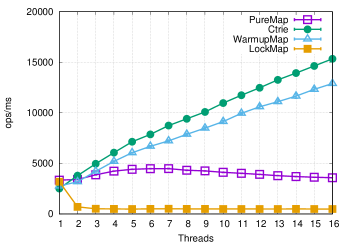
Figure 11. Heating up data. Average throughput of random operations (50% get, 25% insert and 25% delete), each run is 500ms and average over 25 runs.

As we can see from the figure, the PureMap performs best on one thread but scalability is very poor; Ctrie has good scalability; and WarmupMap has better performance than Ctrie in one thread since it remains in the PureMap state (no CAS failures on one thread). Conversely, the adaptive version transitions to Ctrie so it has much better scalability than PureMap. The gap between Ctrie and WarmupMap is due to the cost of transitioning plus the cost of extra indirections in freezable references. As a baseline, we also include a version using the same HashMap but with a coarse-grained lock around the data structure (an MVar in Haskell).

8.2. Parallel freeze+convert

Next, we check that the algorithm described in § 7.1.2 improves the performance of the freeze+convert phase by itself. For example, on 1 thread, the simple preorder traversal takes 3.37s to freeze and convert a 10 million element Ctrie, and the randomized algorithm matches its performance (3.36s). But on 16 threads, the randomized version speeds up to 0.41s for the same freeze plus conversion.

8.3. Cooling down data

In this benchmark, we compare the performance of AdaptiveMap (Ctrie to Pure) against PureMap and Ctrie. No heuristic is used here, the programmer calls the transition method manually based on known or predicted shifts in workload.

We measure the time to complete a fixed number of insert operations (hot phase) or get operations (cold phase), distributed equally over varying number of threads. In Fig. 12, we break these phases down individually, for the AdaptiveMap, running the hot operations when it is in the Ctrie state, and cold operations after it transitions to the PureMap state.

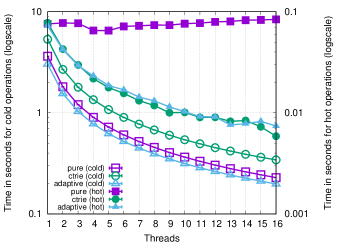
Figure 12. Median time (logscale) over 25 runs for $10^{5}$ hot operations and $2\times 10^{7}$ cold operations, measured separately, with initial size 0, and randomly generated keys in the range $[0,2^{32}]$. Solid dots correspond to the right y-axis, hollow dots correspond to the left y-axis.

We can see that AdaptiveMap closely tracks the performance of Ctrie in the hot phase, and PureMap in the cold phase. Again, the gap between Ctrie and AdaptiveMap shows the overhead of extra indirections in freezable references. Fig. 12 is representative of what happens if the adaptive data structure is put into the correct state before a workload arrives.

In the next benchmark, “hotcold”, we measure the total time to complete a fixed number of operations, divided in a fixed ratio between insert (hot phase) and get (cold phase), with the adaptive data structure transitioning—during the measured runtime—from Ctrie to PureMap, at the point where the hot phase turns to cold. The results are shown in Fig. 13.

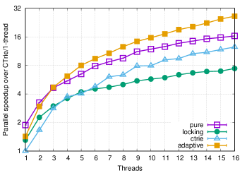
Figure 13. Parallel speedup relative to time taken by Ctrie on a single thread, median over 25 runs, for $10^{5}$ hot operations, followed by transition, and then $2\times 10^{7}$ cold operations, with initial size 0, and randomly generated keys in the range $[0,2^{32}]$

Here the latency of the transition starts out at 0.6ms on a single thread, and reduces to 0.2ms on 16 threads, because more threads can accomplish the freeze/convert faster using the randomized algorithm of § 7.

In this two-phase scenario, because both the non-adaptive variants have to spend time in their “mismatched” workloads, the adaptive algorithm comes out best overall. One interesting outcome is that Ctrie is bested by PureMap in this case. In a scenario of concurrent-reads rather than concurrent-writes, the purely functional, immutable data structure occupies less space and can offer higher read throughput in the cold phase.

Next, we scale the number of operations (and maximum data structure size) rather than the threads. We measure the total time including transition time for a mixed workload of insert (hot) operations followed by transition, then get (cold) operations, keeping the hot-to-cold ratio constant, and varying over the total number of operations, divided equally over a fixed number of threads. The results in Fig. 14 show that AdaptiveMap beats both PureMap and Ctrie on such a workload.

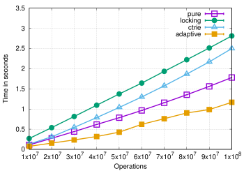
Figure 14. Median time over 25 runs for hot operations followed by transition then cold operations, with hot-to-cold ratio of $1:200$, equally divided over 16 threads, with initial size 0, and randomly generated keys in the range $[0,2^{32}]$

At the right edge of Fig. 14, the data structure grows to contain 500K elements, and transition times are 50ms, which is equivalent to a throughput of 10 million elements-per-second in the freeze and convert step.

8.4. Compacting data

As an additional scenario, we use our technique to build an adaptive data structure that transitions from a PureMap to a CompactMap, which is a PureMap inside a compact region (Yang et al., 2015). Objects inside a compact region are in normal form, immutable, and do not need to be traced by the garbage collector. This is an excellent match for cooling down data; we build a large PureMap (hot phase), and transition to a CompactMap for read operations (cold phase).

We measure total number of bytes copied during garbage collection, for CompactMap, comparing against “No-op” and PureMap. No-Op is no data structure at all, consisting of empty methods. GC is triggered by simulating a client workload, generating random keys using a pure random number generator and looking up values from the map. The map is filled by running insert operations on random keys, followed by transition, and then equally many get operations. The workload is equally divided among 16 worker threads.

The results are shown in Fig. 15. As the number of operations increases, the version that adapts into a compact form has fewer bytes to copy during GC. Even the No-Op version copies some amount, as it runs the client workload (including RNG).

Figure 15. Bytes copied during GC against varying number of operations, averaging over 25 iterations, with hot-to-cold ratio of $1:1$, equally divided over 16 threads, with initial size 0, and randomly generated keys in the range $[0,2^{63}]$

Compacting data provides one example of dealing with a read-heavy phase. Other examples include creating additional caching structures or reorganizing data.

8.5. Shifting hot spots

In this benchmark we consider an idealized document server where one document is hot and others are cold, and these roles change over time. We have 2000 CTrie Int ByteString (each representing a dynamic document, in chunks), for phase $i$ ($i\in[1,2000]$) every thread has a 50% chance to perform a hot operation on $i$-th map, otherwise it chooses a map uniformly at random and performs a (cold) operation. For a hot operation, it is 80% insert and 20% lookup. For a cold operation, it is 80% lookup and 20% insert.

We consider three implementations: first, plain Ctrie; second, Ctrie with QuickLZ to compress the ByteString (and decompress on all lookups), and, third, adaptive map which will transition from Ctrie to Ctrie+QuickLZ after each phase, when a document switches from hot to cold. In this benchmark we use 8 threads—the average latency for a method call is in figure Fig. 16 and the maximum memory residency for the whole run is shown in Fig. 17. According to these results, Ctrie+QuickLZ is significantly slower but saves memory, whereas adaptive map achieves a balance between the two implementations: saving memory without introducing too much overhead.

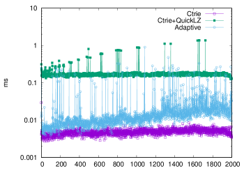
Figure 16. The average latency for each round of 200 operations; y-axis is time in logscale.

Ctrie	Ctrie+QuickLZ	Adaptive
16240 megabytes	7738 megabytes	13194 megabytes

Figure 17. Peak memory usage on server variants.

9. Conclusion

In this paper, we proposed a simple technique that requires a minimum amount of work to add an adaptive capability to existing lock-free data structures. This provides an easy starting point for a programmer to build adaptive lock-free data structures by composition. The hybrid data structure can be further optimized to better serve practical client workloads, as the programmer sees fit.

Freezable references emerged as a useful primitive in this work. In the future, we plan to work on a transition method that preserves lock-freedom without sacrificing performance, and on techniques to automatically detect, or predict, when transition is needed.

Appendix

Appendix A CAS in a purely functional language

Our formal treatment in § 6 benefits from using a purely functional term language which separates effects into a monad. This means, however, that allocation is not a side effect and that pure values lack meaningful pointer identity.

How then to implement compare-and-swap? The trick that Haskell uses is to give values identity by virtue of being pointed to by a mutable reference. As soon as a value is placed in a reference with writeIORef, it becomes the subject of possible CAS operations. We can observe a kind of version of the value by reading the reference and getting back an abstract “ticket” that encapsulates that observation:

⬇

readForCAS :: IORef a $\rightarrow$ IO (Ticket a)

peekTicket :: Ticket a $\rightarrow$ a

So while we may not be able to distinguish whether one value of type a has the same “pointer identity” as another, we can distinguish whether the value in the IORef has changed since a ticket was read. And our CAS operation then uses a ticket in lieu of the “old” value in machine-level CAS:

⬇

casIORef :: IORef a $\rightarrow$ Ticket a $\rightarrow$ a

$\rightarrow$ IO (Bool, Ticket a)

Unlike machine-level CAS, this operation returns two values: first, a flag indicating whether the operation succeeded, and, second, a ticket to enable future operations. In a successful CAS, this is the ticket granted to the “new” value written to the memory cell.

A.1. Physical Equality and Double Indirection

The above semantics for CAS depends on a notion of value equality, e.g., where we test $H(\ell)=old$. However, atomic memory operations in real machines work on single words of memory. Thus, physical, pointer equality is the natural choice for a language incorporating CAS. But, as described in Appendix A, this is at odds with a purely functional language which does not have a built-in notion of pointer identity or physical equality. (This is also reflected in the fact that the separate, pure, term reduction (Fig. 9) makes no use of the heap, $H$, and does not mention locations $\ell$.)

How do we square this circle? The basic solution is to introduce a mechanism to selectively create a meaningful pointer identity for values which we wish to store in atomically-updated references. The concept of a “Ticket” shown in Appendix A is the the approach used by the Haskell atomic-primops library that exposes CAS to users. It uses a GHC-specific mechanism for establishing meaningful pointer equality and preventing compiler optimizations (such as unboxing and re-boxing) that would change it.

In our simple formal language we instead restrict CAS to operate on references containing scalars, values representable as a machine word. In particular, we consider both locations $\ell$ and integers $n$ to be scalar values. Accordingly, we use a restricted typing rule for casRef, shown in Fig. 8.

Because we can perform CAS on locations, we can enable a similar approach as the atomic-primops library using double indirection. That is, because references already correspond to heap locations, simply storing a value $v$ in a reference, allows us to use its location $\ell$ in lieu of $v$. For instance, $\ref{(}\textsf{Int},\textsf{Int})$ would not support atomic modification, whereas $\ref{(}\ref{(}\textsf{Int},\textsf{Int}))$ would allow us to achieve the desired effect.

To follow this protocol, pure values to be used with CAS must be “promoted” to references with newRef (references which are never subsequently modified). As part of our implicit desugaring to our core language, we treat all CAS operations on non-scalar types as implicitly executing a newRef first. For instance, the root of the hybrid data structure must be treated thus, because it stores compound data values such as (AB _ _). In the operational semantics of the next section, this means that CAS operations on such types consume two time steps instead of one, which is immaterial to establishing upper bounds for progress (lock-freedom).

Appendix B Freezable References: Implementation

Fig. 19 gives a Haskell definition for a freezable reference as a wrapped IORef. It is nothing but an IORef plus one extra bit of information, indicating frozen status. We also define an exception CASFrznExn, which is raised when a thread attempts a CAS operation on a frozen IORef. This implementation adds an extra level of indirection, but as a result it can be atomically modified or atomically frozen by changing one physical memory location. An implementation with compiler support might, for example, use pointer tagging to store the frozen bit.

Fig. 19 shows our freezeIORef function. Once this succeeds, the reference is marked as frozen and no further modification is allowed. Any attempt to modify a frozen IORef will raise the exception CASFrznExn.

We wrap and re-export relevant functions in Data.IORef, such as writeIORef and atomicModifyIORef, so that a freezable IORef can be used without any code modifications—only a change of module imported. We also provide all functions related to IORef in Data.Atomics, such as casIORef. The implementation of these functions is straightforward; they are easily written by pattern matching on the wrapper IOVal. Read operations ignore the frozen bit, but write operations throw an exception when applied to a frozen reference.

⬇

module Data.IORef.Freezable ($\cdots$) where

import qualified Data.IORef as IR

import Control.Monad.Except

newtype IORef t = IORef (IR.IORef (IOVal t))

data IOVal t = Val t $\mid$ Frozen t

data CASFrznExn = CASFrznExn

deriving (Show, Exception)

Figure 18. Definition of the freezable variant of IORef.

⬇

74freezeIORef r = loop r =<< readForCAS r

75 where

76 loop ref tik = do

77 (flag, tik') $\leftarrow$ tryFreezeIORef ref tik

78 unless flag (loop ref tik')

79

80tryFreezeIORef :: IORef a

81 $\rightarrow$ Ticket (IOVal a)

82 $\rightarrow$ IO (Bool, Ticket (IOVal a))

83tryFreezeIORef (IORef ref) tik = do

84 case peekTicket tik of

85 Frozen _ $\rightarrow$ return (True, tik)

86 Val a $\rightarrow$ A.casIORef ref tik (Frozen a)

Figure 19. Freeze or attempt to freeze a single reference

Appendix C Correctness Proof

Theorem C.1.

If data structures A and B are lock-free, then the hybrid data structure built from A and B is also lock-free.

Proof.

For any configuration of the hybrid data structure, $\sigma^{Hybrid}\allowbreak=(t,H,F,M^{+},\mathcal{T}r,\mathcal{P})$, and schedule $\pi$, there exists an upper bound function $f$ such that, some thread $\tau_{j}\in\mathfrak{T}{}$ will finish executing method $m_{i}\in M^{+}$ in $f(\sigma^{Hybrid})$ timesteps.

We use shorthands $\sigma^{A}$ and $\sigma^{B}$ to refer to projections of $\sigma^{Hybrid}$ that take only the subset of the state relevant to the A or B structures, i.e. viewing $\sigma^{Hybrid}$ as though it were an A. Likewise, $H_{A}$ and $H_{B}$ refer to projections of the heap, $H_{Hybrid}$.

Further, to account for the extra read (i.e. CAS) at the beginning of each hybrid method on line 44, we abbreviate $f_{A}^{\prime}(x)=f_{A}(x)+|\mathfrak{T}|$ to refer to the updated bound on A (and likewise for $f_{B}^{\prime}$). The reason the increase is proportional to the number of threads, is that an adversarial scheduler can cause each thread to spend one operation here before getting to any actual calls to A’s methods.

To define $f(\sigma^{Hybrid})$, here we reason by cases over the current state, $\sigma^{Hybrid}$. There are three cases to consider based on the current state of the heap, $H_{Hybrid}$:

• A state: $H(H(\ell_{hy}))$ is an $A$ value :

For methods other than transition, by the lock-freedom of data structure A, there must be some method which finishes execution in $f_{A}^{\prime}(|H_{A}|)$ timesteps. This bound, representing A’s lock-freedom, holds if there is no thread which executes transition and passes line 49 on or before time $t+f_{A}^{\prime}(|H_{A}|)+2$. Here the additional “$+2$” addresses the fact that the original method may throw an exception on the very last time step during which it would have succeeded, and then require two more time steps to cross line 49.

If a thread passes line 49 in time $t^{\prime}$, such that $t^{\prime}\leq t+f_{A}^{\prime}(|H_{A}|)+2$, and the configuration at that time is $\sigma^{Hybrid}_{t^{\prime}}=(t^{\prime},H^{\prime},F,M^{+},\allowbreak\mathcal{T}r^{\prime},\mathcal{P}^{\prime})$ where $H(H(\ell_{hy}))$ is an $AB$ value, then the time for a transition or another method to subsequently complete is bounded by $f_{tran}(|H_{Hybrid}|+t^{\prime}-t)$—where $f_{tran}$ will be defined below in the next case. So, we have $f(|H_{Hybrid}|)=f_{A}^{\prime}(|H_{A}|)+2+f_{tran}(|H_{Hybrid}|+t^{\prime}-t)$.

• AB state: $H(H(\ell_{hy}))$ is an $AB$ value :

We reach this state only if some thread executing transition already passed line 49, and none of the threads executing transition pass the linearization points at lines 54 or 59. In this state, we have $K\geq 1$ threads executing transition and $K^{\prime}\geq 0$ threads executing other methods in $\mathcal{P}{}$.

If the scheduler only schedules the $K^{\prime}$ threads executing methods other than transition — never entering line 47 — then some method will finish execution in $f_{A}^{\prime}(|H_{A}|)$ timesteps. Otherwise, at least some thread takes a step inside transition. Examining Fig. 5, if thread $\tau_{j}$ tries to $cas(\ell,\_,\_)$ where $\ell\in F$, it will raise an exception, and according to line 54, this causes $\tau_{j}$ to start executing transition, so the next time it gets scheduled, the configuration of $\sigma^{A}$ in the future will behave as if the scheduler never scheduled $\tau_{j}$. Any new method call entering the picture, according to line 47, will just call transition. Since there are only $|\mathfrak{T}{}|$ threads, after $|\mathfrak{T}{}|\times f_{A}^{\prime}(|H_{A}|)$ timesteps, either every thread is executing transition, or some method other than transition completes. For each timestep, at most one new memory cell can be allocated, so if no method completes, the heap size of $\sigma^{A}$ is at most $|H_{A}|+|\mathfrak{T}{}|\times f_{A}^{\prime}(|H_{A}|)$.

After the first thread does a successful CAS on line 49, the address $H(\ell_{hy})$ will not change until some thread is on line 54 or 59, and tries to CAS $H(\ell_{hy})$. The first thread that executes this CAS must succeed because $\ell_{hy}\notin F$, and the old value is the current value in the heap. Since the runtimes of freeze and convert only depend on the heap size, some thread must finish executing freeze (lines 52 or 57) in $|\mathfrak{T}{}|\times(f_{frz}(|H_{A}|+|\mathfrak{T}{}|\times f_{A}^{\prime}(|H_{A}|)))$ timesteps, and then convert (lines 53 or 58) in $|\mathfrak{T}{}|\times(f_{conv}(|H_{A}|+|\mathfrak{T}{}|\times f_{A}^{\prime}(|H_{A}|)))+1$ timesteps. Finally threads must then must attempt the CAS in lines 54 or 59. After all freezes and conversions have completed, a thread can only fail at these lines if another succeeds, and so in the very next timestep one thread must succeed in changing the state to B. This last CAS is the linearization point and completes the transition. So after

$$f_{tran}(|H_{Hybrid}|) =|\mathfrak{T}{}|\times(f_{frz}(|H_{A}|+|\mathfrak{T}{}|\times f_{A}^{\prime}(|H_{A}|)))$$

$$+|\mathfrak{T}{}|\times(f_{conv}(|H_{A}|+|\mathfrak{T}{}|\times f_{A}^{\prime}(|H_{A}|)))$$

$$+|\mathfrak{T}{}|\times f_{A}^{\prime}(|H_{A}|)+1$$

timesteps, either a data structure method completes or some thread finishes the transition method.

• B state: $H(H(\ell_{hy}))$ is a $B$ value :

If a thread calls transition at this state, execution passes through line 60 and the transition finishes executing immediately. Further completing this method constitutes progress vis-à-vis lock freedom.

Other new method calls execute line 49, thus calling the corresponding method from $\sigma_{B}$. By lock-freedom on data structure B, there must be some method that finishes execution in $f_{B}^{\prime}(|H_{B}|)$ timesteps. But some time may be wasted on threads that have not yet finished executing transition. Being in the B state means that at least one thread has completed a transition, but there may be others ongoing. These ongoing transitions will finish in $f_{tran}(|H_{Hybrid}|)$ timesteps.

For those methods executing inside the B code (line 49) we have the bound from B, $f_{B}^{\prime}(|H_{B}|)$. Methods executing the A code (line 46) raise an exception in $f_{A}^{\prime}(|H_{A}|)$ steps when they try to commit with a CAS (or earlier). Methods which follow that exception path, according to line 55, fall back under the B case after wasting some steps to get there. So we have, $f_{Hybrid}(|H_{Hybrid}|)=f_{A}^{\prime}(|H_{A}|)+f_{tran}(|H_{Hybrid}|)+f_{B}^{\prime}(|H_{B}|)$.

We defined the upper bound function $f(\sigma^{Hybrid})$ for these three cases, which concludes the proof. ∎

Theorem C.2.

If $\sigma^{B}\approx\sigma^{Hybrid}$ where $\sigma^{B}=(t_{B},H_{B},\_,M,\allowbreak{\mathcal{T}r}_{B},{\mathcal{P}}_{B})$, $\sigma^{Hybrid}=(t,H_{Hybrid},\_,M^{+},\_,{\mathcal{P}}_{Hybrid})$ and ${\mathcal{P}}_{B}$ is obtained by removing all transition method calls in ${\mathcal{P}}_{Hybrid}$, then for any scheduler $\pi$, there exists a scheduler $\pi^{\prime}$ such that, if $\sigma^{Hybrid}\rightarrow_{\pi}\sigma^{Hybrid}_{1}$ then ${\sigma^{B}}\twoheadrightarrow_{\pi^{\prime}}\sigma^{B}_{1}$, where $\sigma^{B}_{1}\approx\sigma^{Hybrid}_{1}$.

Here, we do not need a fine-grained correspondence between intermediate steps of Hybrid and $B$ methods. Rather, $\mathcal{P}_{B}$ contains a pristine copy of method $m_{i}$ for each method expression sharing the same label in $\mathcal{P}_{Hybrid}$—irrespective of whether it is already partially evaluated within $\mathcal{P}_{Hybrid}$. Whereas original methods $\textsf{method}_{m_{i}}\,\{\;e\;\}$ are replaced by pristine $B$ versions, transition calls are instead replaced by “No-Ops”, i.e. return (). It is only when the hybrid data structure completes a method that we must reduce $B$ to match the hybrid.

Proof.

Assume $\pi(t)=\tau$, and $\sigma^{Hybrid}\rightarrow_{\pi}\sigma^{Hybrid}_{1}$ where $\sigma^{Hybrid}_{1}\allowbreak=(t+1,H_{Hybrid_{1}},\_,M^{+},\_)$. We proceed by analyzing the four cases according to Fig. 10.

• NEW: Let $\pi^{\prime}=\pi$ and $\sigma^{B}_{1}=\sigma^{B}$. Since this is not a linearization point, we have $\sigma^{B}\approx\sigma^{Hybrid}_{1}$ and ${\sigma^{B}}\rightarrow_{\pi}^{0}\sigma^{B}$.

• METHODFINISH($m$):

  • $m\equiv$ transition: Same as the NEW case, by the property of conversion, $\sigma^{Hybrid}\approx\sigma^{Hybrid}_{1}$.

  • $m\equiv m_{i}$: Let

    $$\pi^{\prime}(t)=\begin{cases}\tau&\text{for }t_{B}\leq t\leq t^{\prime\prime}\\ \pi(t)&\text{otherwise}\end{cases}$$

    Then,

    $${\sigma^{B}} \to_{\pi^{\prime}}\sigma^{B}_{0}=(t_{B}+1,{H_{B}}^{\prime},F_{B}^{\prime},M,{\mathcal{T}r}_{B},\mathcal{P}_{B_{0}})$$

    $$\twoheadrightarrow_{\pi^{\prime}}{\sigma^{B}_{0}}^{\prime}=(t^{\prime\prime}-1,{H_{B}}^{\prime\prime},F_{B}^{\prime\prime},M,{\mathcal{T}r}_{B},\mathcal{P}_{B_{0}^{\prime}})$$

    $$\to_{\pi^{\prime}}\sigma^{B}_{1}=(t^{\prime\prime},{H_{B}}^{\prime\prime\prime},F_{B}^{\prime\prime\prime},M,{\mathcal{T}r}_{B}+\kern-5.59721pt+\kern 3.44444pt[(m_{i},\_)],\mathcal{P}_{B_{0}^{\prime\prime}})$$

    So, $\pi^{\prime}(t)$ initiates sequential execution of $m_{i}$. Since $\sigma^{B}\approx\sigma^{Hybrid}$, we have $\sigma^{B}_{1}\approx\sigma^{Hybrid}_{1}$.

• CAS: Same as the NEW case. Note that if $cas$ fails and raises exception at line 54, we know that $\tau_{j}$ will call $m_{i}$ once it finishes executing transition. But this is an internal matter; because this recursion happens inside a top-level $\textsf{method}_{m_{i}}\,\{\;\;\}$ form, the corresponding $m_{i}^{B}$ method does not update.

• FRZ: Same as the NEW case.

• METHODPURE: Same as the NEW case.

∎

- (1)
- Afek et al. (1993) Yehuda Afek, Hagit Attiya, Danny Dolev, Eli Gafni, Michael Merritt, and Nir Shavit. 1993. Atomic Snapshots of Shared Memory. J. ACM 40, 4 (Sept. 1993), 873–890. DOI:http://dx.doi.org/10.1145/153724.153741
- Agrawal et al. (2010) Kunal Agrawal, Charles E. Leiserson, and Jim Sukha. 2010. Helper Locks for Fork-join Parallel Programming. In Proceedings of the 15th ACM SIGPLAN Symposium on Principles and Practice of Parallel Programming (PPoPP ’10). ACM, New York, NY, USA, 245–256. DOI:http://dx.doi.org/10.1145/1693453.1693487
- Bagwell (2001) Phil Bagwell. 2001. Ideal Hash Trees. Es Grands Champs 1195 (2001).
- Bauman et al. (2015) Spenser Bauman, Carl Friedrich Bolz, Robert Hirschfeld, Vasily Kirilichev, Tobias Pape, Jeremy G. Siek, and Sam Tobin-Hochstadt. 2015. Pycket: A Tracing JIT for a Functional Language. In Proceedings of the 20th ACM SIGPLAN International Conference on Functional Programming (ICFP 2015). ACM, New York, NY, USA, 22–34. DOI:http://dx.doi.org/10.1145/2784731.2784740
- Bolz et al. (2013) Carl Friedrich Bolz, Lukas Diekmann, and Laurence Tratt. 2013. Storage Strategies for Collections in Dynamically Typed Languages. SIGPLAN Not. 48, 10 (Oct. 2013), 167–182. DOI:http://dx.doi.org/10.1145/2544173.2509531
- De Wael et al. (2015) Mattias De Wael, Stefan Marr, Joeri De Koster, Jennifer B. Sartor, and Wolfgang De Meuter. 2015. Just-in-time Data Structures. In 2015 ACM International Symposium on New Ideas, New Paradigms, and Reflections on Programming and Software (Onward!) (Onward! 2015). ACM, New York, NY, USA, 61–75. DOI:http://dx.doi.org/10.1145/2814228.2814231
- Gordon et al. (2012) Colin S. Gordon, Matthew J. Parkinson, Jared Parsons, Aleks Bromfield, and Joe Duffy. 2012. Uniqueness and Reference Immutability for Safe Parallelism. SIGPLAN Not. 47, 10 (Oct. 2012), 21–40. DOI:http://dx.doi.org/10.1145/2398857.2384619
- Gramoli (2015) Vincent Gramoli. 2015. More Than You Ever Wanted to Know About Synchronization: Synchrobench, Measuring the Impact of the Synchronization on Concurrent Algorithms. In Proceedings of the 20th ACM SIGPLAN Symposium on Principles and Practice of Parallel Programming (PPoPP 2015). ACM, New York, NY, USA, 1–10. DOI:http://dx.doi.org/10.1145/2688500.2688501
- Harris (2001) Timothy L. Harris. 2001. A Pragmatic Implementation of Non-blocking Linked-Lists. In Proceedings of the 15th International Conference on Distributed Computing (DISC ’01). Springer-Verlag, London, UK, UK, 300–314. http://dl.acm.org/citation.cfm?id=645958.676105
- Harris et al. (2002) Timothy L. Harris, Keir Fraser, and Ian A. Pratt. 2002. A Practical Multi-word Compare-and-Swap Operation. In Proceedings of the 16th International Conference on Distributed Computing (DISC ’02). Springer-Verlag, London, UK, UK, 265–279. http://dl.acm.org/citation.cfm?id=645959.676137
- Hendler et al. (2004) Danny Hendler, Nir Shavit, and Lena Yerushalmi. 2004. A Scalable Lock-free Stack Algorithm. In Proceedings of the Sixteenth Annual ACM Symposium on Parallelism in Algorithms and Architectures (SPAA ’04). ACM, New York, NY, USA, 206–215. DOI:http://dx.doi.org/10.1145/1007912.1007944
- Herlihy et al. (2003a) Maurice Herlihy, Victor Luchangco, and Mark Moir. 2003a. Obstruction-Free Synchronization: Double-Ended Queues As an Example. In Proceedings of the 23rd International Conference on Distributed Computing Systems (ICDCS ’03). IEEE Computer Society, Washington, DC, USA, 522–. http://dl.acm.org/citation.cfm?id=850929.851942
- Herlihy et al. (2003b) Maurice Herlihy, Victor Luchangco, Mark Moir, and William N. Scherer, III. 2003b. Software Transactional Memory for Dynamic-sized Data Structures. In Proceedings of the Twenty-second Annual Symposium on Principles of Distributed Computing (PODC ’03). ACM, New York, NY, USA, 92–101. DOI:http://dx.doi.org/10.1145/872035.872048
- Herlihy and Wing (1990) Maurice P. Herlihy and Jeannette M. Wing. 1990. Linearizability: A Correctness Condition for Concurrent Objects. ACM Trans. Program. Lang. Syst. 12, 3 (July 1990), 463–492. DOI:http://dx.doi.org/10.1145/78969.78972
- Kilpatrick et al. (2014) Scott Kilpatrick, Derek Dreyer, Simon Peyton Jones, and Simon Marlow. 2014. Backpack: retrofitting Haskell with interfaces. In ACM SIGPLAN Notices, Vol. 49. ACM, 19–31.
- Kusum et al. (2016) Amlan Kusum, Iulian Neamtiu, and Rajiv Gupta. 2016. Safe and Flexible Adaptation via Alternate Data Structure Representations. In Proceedings of the 25th International Conference on Compiler Construction (CC 2016). ACM, New York, NY, USA, 34–44. DOI:http://dx.doi.org/10.1145/2892208.2892220
- Leino et al. (2008) K. Rustan Leino, Peter Müller, and Angela Wallenburg. 2008. Flexible Immutability with Frozen Objects. In Proceedings of the 2Nd International Conference on Verified Software: Theories, Tools, Experiments (VSTTE ’08). Springer-Verlag, Berlin, Heidelberg, 192–208. DOI:http://dx.doi.org/10.1007/978-3-540-87873-5_17
- Marlow et al. (2011) Simon Marlow, Ryan R. Newton, and Simon Peyton Jones. 2011. A monad for deterministic parallelism. In Proceedings of the 4th ACM symposium on Haskell (Haskell ’11). ACM, 71–82.
- Nawab et al. (2015) Faisal Nawab, Dhruva R Chakrabarti, Terence Kelly, and Charles B Morrey III. 2015. Procrastination Beats Prevention: Timely Sufficient Persistence for Efficient Crash Resilience.. In EDBT. 689–694.
- Newton et al. (2015) Ryan R. Newton, Peter P. Fogg, and Ali Varamesh. 2015. Adaptive Lock-free Maps: Purely-functional to Scalable. In Proceedings of the 20th ACM SIGPLAN International Conference on Functional Programming (ICFP 2015). ACM, New York, NY, USA, 218–229. DOI:http://dx.doi.org/10.1145/2784731.2784734
- Nikhil (1991) Rishiyur S. Nikhil. 1991. ID Language Reference Manual. (1991).
- Peyton Jones et al. (1996) Simon Peyton Jones, Andrew Gordon, and Sigbjorn Finne. 1996. Concurrent Haskell. In Proceedings of the 23rd ACM SIGPLAN-SIGACT Symposium on Principles of Programming Languages (POPL ’96). ACM, New York, NY, USA, 295–308. DOI:http://dx.doi.org/10.1145/237721.237794
- Peyton Jones et al. (1999) Simon Peyton Jones, Alastair Reid, Fergus Henderson, Tony Hoare, and Simon Marlow. 1999. A semantics for imprecise exceptions. In ACM SIGPLAN Notices, Vol. 34. ACM, 25–36.
- Prokopec et al. (2012) Aleksandar Prokopec, Nathan Grasso Bronson, Phil Bagwell, and Martin Odersky. 2012. Concurrent Tries with Efficient Non-blocking Snapshots. In Proceedings of the 17th ACM SIGPLAN Symposium on Principles and Practice of Parallel Programming (PPoPP ’12). ACM, New York, NY, USA, 151–160. DOI:http://dx.doi.org/10.1145/2145816.2145836
- Shalev and Shavit (2006) Ori Shalev and Nir Shavit. 2006. Split-ordered Lists: Lock-free Extensible Hash Tables. J. ACM 53, 3 (May 2006), 379–405. DOI:http://dx.doi.org/10.1145/1147954.1147958
- Vollmer et al. (2017) Michael Vollmer, Ryan G. Scott, Madan Musuvathi, and Ryan R. Newton. 2017. SC-Haskell: Sequential Consistency in Languages that Minimize Mutable Shared Heap. In To appear in the proceedings of the 22st ACM SIGPLAN Symposium on Principles and Practice of Parallel Programming (PPoPP ’17). ACM, New York, NY, USA.
- Xu (2013) Guoqing Xu. 2013. CoCo: Sound and Adaptive Replacement of Java Collections. In Proceedings of the 27th European Conference on Object-Oriented Programming (ECOOP’13). Springer-Verlag, Berlin, Heidelberg, 1–26. DOI:http://dx.doi.org/10.1007/978-3-642-39038-8_1
- Yang et al. (2015) Edward Z. Yang, Giovanni Campagna, Ömer S. Ağacan, Ahmed El-Hassany, Abhishek Kulkarni, and Ryan R. Newton. 2015. Efficient Communication and Collection with Compact Normal Forms. In Proceedings of the 20th ACM SIGPLAN International Conference on Functional Programming (ICFP 2015). ACM, New York, NY, USA, 362–374. DOI:http://dx.doi.org/10.1145/2784731.2784735