Ionized gas in the Scutum spiral arm as traced in [N ii] and [C ii]

Abstract

Context. The warm ionized medium (WIM) occupies a significant fraction of the Galactic disk. Determining the WIM properties at the leading edge of spiral arms is important for understanding its dynamics and cloud formation.

Aims. To derive the properties of the WIM at the inner edge of the Scutum arm tangency, which is a unique location in which to disentangle the WIM from other components, using the ionized gas tracers C⁺ and N⁺.

Methods. We use high spectral resolution [C ii] 158 $\mu$m and [N ii] 205 $\mu$m fine structure line observations taken with the upGREAT and GREAT instruments, respectively, on SOFIA, along with auxiliary H i and ¹³CO observations. The observations consist of samples in and out of the Galactic plane along 18 lines of sight (LOS) between longitude 30^∘ and 32^∘.

Results. We detect strong [N ii] emission throughout the Scutum tangency. At $V_{LSR}$ = 110 to 125 km s^-1 where there is little, if any, ¹³CO, we are able to disentangle the [N ii] and [C ii] emission that arises from the WIM at the arm’s inner edge. We find an average electron density $\sim$0.9 cm^-3 in the plane, and $\sim$0.4 cm^-3 just above the plane. The [N ii] emission decreases exponentially with latitude with a scale height $\sim$55 pc. For $V_{LSR}<$110 km s^-1 there is [N ii] emission tracing highly ionized gas throughout the arm’s molecular layer. This ionized gas has a high density, $n$(e) $\sim$30 cm^-3, and a few percent filling factor. We also find evidence for [C ii] absorption by foreground gas.

Conclusions. [N ii] and [C ii] observations at the Scutum arm tangency reveal a highly ionized gas with average electron density about 10 to 20 times those of the interarm WIM, and is best explained by a model in which the interarm WIM is compressed as it falls into the potential well of the arm. The widespread distribution of [N ii] in the molecular layers shows that high density ionized gas is distributed throughout the Scutum arm. The electron densities derived from [N ii] for these molecular cloud regions are $\sim$30 cm^-3, and probably arise in the ionized boundary layers of clouds. The [N ii] detected in the molecular portion of the spiral arm arises from several cloud components with a combined total depth $\sim$8 pc. This [N ii] emission most likely arises from ionized boundary layers, probably the result of the shock compression of the WIM as it impacts the arm’s neutral gas, as well as from extended H ii regions.

1 Introduction

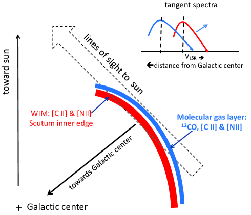
The interstellar medium (ISM) is a dynamic environment in which gas cycles from a diffuse ionized state to dense star forming molecular clouds and back. Stars and supernovae provide energy to disrupt and ionize the gas and generate dynamical flows within and above the disk. Spiral density waves at the leading edge of the arm compress the ionized interarm gas and initiate one of the processes of cloud formation. The dynamics of the arm and the energy sources within the arm determine the distribution of different interstellar gas components within and above the disk. The study of the spiral density waves is thus important for understanding how clouds form and galaxies evolve. The spiral tangent regions are ideal laboratories to study the interaction of the interstellar gas and spiral density waves in the Milky Way as they provide a unique viewing geometry with large enough path lengths to detect the diffuse (atomic or ionized) spiral arm components. This unique viewing geometry of a spiral arm is illustrated in Figure 1 for the Scutum tangency (adapted from Figure 6 in Velusamy et al. (2015)) in which the different gas layers, ionized, atomic, and molecular are shown along with their emission line profiles as a function of $V_{LSR}$. These tangencies are located at $l$ $\sim$ 31^∘, 51^∘, 284^∘, 310^∘, 328^∘, and 339^∘ (Vallée 2008), although there is some scatter, $\sim$4^∘, in the identification of the location of the tangency depending on which tracer is used.

The atomic and molecular components of the ISM in the spiral arms are well traced in emission by H i and CO, respectively, but the photon dominated regions (PDR), CO-dark H₂ and the ionized gas has been less well studied in emission owing to the difficulty of observing key tracers from the ground. The fine-structure transition of ionized carbon, [C ii], at 158 $\mu$m, traces almost all the warm (T$>$ 35K) portions of the ionized ISM. However, [C ii] alone cannot distinguish fully ionized hydrogen gas from weakly ionized gas (carbon ionized but hydrogen neutral). In contrast, nitrogen, with its 14.53 eV ionization potential, has fine-structure lines, [N ii], at 122 $\mu$m and 205 $\mu$m that arise only in highly ionized regions. Here we investigate the influence of the spiral arms on the distribution and dynamics of the highly ionized gas in and out of the plane by observing velocity resolved [N ii] 205 $\mu$m and [C ii] 158 $\mu$m emission in the Scutum spiral arm tangency ($l\sim$ 31^∘), taken with the German Receiver for Astronomy at Terahertz Frequencies (GREAT; Heyminck et al. 2012) and the upGREAT¹ array (Risacher et al. 2016), respectively, onboard the NASA/DLR Stratospheric Observatory for Infrared Astronomy (SOFIA; Young et al. 2012).

The large-scale structure of spiral arms in the Milky Way is a subject of great interest for understanding the dynamics of the Galaxy and for interpreting its properties. Modeling the Galactic spiral structure is based in part on data at the spiral arm tangents in different gas and stellar tracers. However, each of these tracers can occupy a separate lane across the arm reflecting the evolution of gas from low- to high-density clouds as they are swept into the arm’s gravitational potential. Using Herschel HIFI [C ii] maps along with H i and CO maps, Velusamy et al. (2012, 2015) showed that the gas in the Scutum, Crux, Norma, and Perseus arms was arranged in layers and revealed an evolutionary transition from lowest to highest density states. In particular the geometry of the tangencies made possible the detection of the low density WIM in [C ii] and revealed a higher density WIM at the inner edge of the arm than in the interarm gas. They suggested this increase was a result of the compression of the WIM at the leading edge. Here we use both [C ii] and [N ii] observations of the Scutum arm tangency at $l\sim$31^∘ to study the interaction of the spiral arm potential with the ionized interarm gas.

Figure 1: Schematic view of the Scutum spiral arm tangency showing the structure of the gas layers (adapted from Figure 6 in Velusamy et al. (2015). The emission of key gas tracers along the tangency, [C ii], [N ii], and CO help distinguish the WIM and molecular gas layers indicated as red and blue colors, respectively. Note the long path length along the tangency which improves the sensitivity to the weak [C ii] and [N ii] emission from the WIM. A schematic of the velocity ($V_{LSR}$) profile (shown in the inset) of the corresponding spectral line intensities for each layer, demonstrates why it is possible to separate the emission from the WIM from the neutral gas components. Note that this cartoon is intended to be a schematic and is not to scale.

This paper is organized as follows. In Section 2 we present the observations and data reduction, while in Section 3 we describe the distribution of [C ii] and [N ii] in the Scutum tangency. In Section 4 we derive the properties of the ionized gas, including density and scale height, using [C ii] and [N ii], and discuss the possible mechanisms responsible for the distribution of [N ii]. Section 5 summarizes the results.

2 Observations

The Scutum arm is located about 4 kpc from the Galactic Center and wraps more than half way around the Galaxy. In Figure 2 we show a ¹³CO longitude–velocity map of the tangency near $l\sim$31^∘ and have marked the inner and outer tangencies derived from Reid et al. (2016) with black lines. The ¹³CO traces the molecular clouds in this region. The ¹³CO ($l$–$V_{LSR}$) map at Galactic latitude, $b$ = 0^∘ is derived from the Galactic Ring Survey (GRS) data (Jackson et al. 2006).

Figure 2: A ¹³CO longitude–velocity plot of the Scutum arm in the region $l\sim$29^∘ to 33^∘ at $b$=0^∘, where we mark the inner (black solid line) and outer (dashed black line) tangencies taken from Reid et al. (2016) using their fit to the near–far distances. The arrows at the bottom indicate Galactic longitudes of the lines of sight observed in [C ii] and [N ii] with upGREAT and GREAT, respectively.

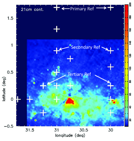
To compare the spatial and velocity structure of the spiral arm gas components in both the molecular (neutral) and the ionized gases in the Scutum arm we made small–scale cross maps of [C ii] and [N ii] in longitude along and in latitude above a spiral arm tangency with the GREAT single pixel receiver for [N ii] and the upGREAT 7-pixel array for [C ii]. The [N ii] and [C ii] emission across the arm allows us to examine the impact of the spiral arm potential on the ionized gas components. To examine the spatial and velocity structures of these gas components across the tangency and perpendicular to the Galactic plane we observed [N ii] and [C ii] along 18 lines of sight (LOS) across the Scutum tangency from 30$\aas@@fstack{\circ}$0 to 31$\aas@@fstack{\circ}$75 covering $b$ from -0$\aas@@fstack{\circ}$25 to 1$\aas@@fstack{\circ}$7. These 18 LOS are indicated in Figure 2 by crosses superimposed on a 21 cm continuum map (Stil et al. 2006) of the Scutum tangency region. We have also indicated the primary, secondary, and tertiary reference sky positions used in the observations (see discussion below).

Figure 3: The 18 lines of sight observed in [C ii] and [N ii] are indicated by white crosses superimposed on a 21 cm continuum map of the Scutum tangency region (Stil et al. 2006). The primary reference off positions are labeled as are the secondary and tertiary reference positions.

We observed the Scutum tangency in the ionized carbon (C⁺) ²P_3/2 – ²P_1/2 fine structure line, [C ii], at 1900.5369 GHz ($\lambda\sim$157.741 $\mu$m), using upGREAT (Risacher et al. 2016) and the ionized nitrogen (N⁺) ³P₁–³P₀ fine structure line, [N ii], at 1461.1338 GHz $(\lambda\sim$ 205.178 $\mu$m) using GREAT (Heyminck et al. 2012) onboard SOFIA (Young et al. 2012). The upper state of C⁺, ²P_3/2, lies at an energy, $E$/k, about 91.2 K above the ground state, and the upper states of N⁺, ³P₁ and ³P₂, lie at 70.1 K and 188.2 K, respectively, above the ground state. Our program (proposal ID 04_0033; PI Langer) was part of the Guest Observer Cycle 4 campaign. The observations were made between May 12 and June 10, 2016 on six flights spread over SOFIA flights #296 to #308. Both [C ii] and [N ii] spectra were observed simultaneously in GREAT configuration: LFA+H+V/L1 with [C ii] in LFA:LSB and [N ii] in L1:USB. The typical observing time on each target was in the range of 15 to 30 minutes.

[C ii] and [N ii] are widespread throughout the Galaxy so finding a clean off position for proper calibration is a challenge in observing the Scutum spiral arm. The telescope on SOFIA cannot slew more than 0$\aas@@fstack{\circ}$4 to 0$\aas@@fstack{\circ}$8 from the ON to the OFF position, and it was thus necessary to observe [C ii] and [N ii] in a series of steps in $b$ starting at a latitude where the emission is weak enough to provide a clean OFF position. In practice even the largest $b$ value was not always absolutely clean of emission, but it was generally weak enough to use as a reference position. The observing scenario, therefore, used a set of primary, secondary and tertiary reference positions located at $b$ = 1$\aas@@fstack{\circ}$7, 0$\aas@@fstack{\circ}$9, and 0$\aas@@fstack{\circ}$25, respectively as shown in Figure 3. The primary reference positions, the LOSs at $b$=1$\aas@@fstack{\circ}$7, were observed with respect to an OFF position at $b$=2$\aas@@fstack{\circ}$1 at the same longitude. These LOS at ($l$,$b$) = (30$\aas@@fstack{\circ}$0,1$\aas@@fstack{\circ}$7) and (31$\aas@@fstack{\circ}$0,1$\aas@@fstack{\circ}$7) were then used as primary reference positions for observations at lower values of $b$, two of which at $b$= 0$\aas@@fstack{\circ}$9 then could be used as secondary reference positions (see Figure 3) for LOS at yet lower values of $b$. This procedure was repeated one more time and a set of tertiary reference positions were established at $b$ = 0$\aas@@fstack{\circ}$75 (see Figure 3). In this scheme each target LOS used the nearest (up to within 0$\aas@@fstack{\circ}$8) primary/secondary/tertiary reference position. The calibrated emission spectra at the reference positions were than added incrementally in a hierarchical manner to the respective target spectra.

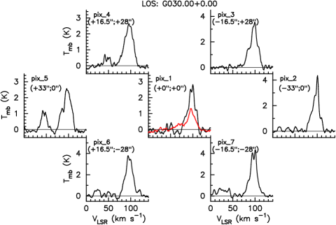
The dual-polarization 7-pixel upGREAT array has a FWHM beam size of 14^′′ at 1.9 THz. The array is arranged in a hexagonal pattern with a central beam. The beam spacing is approximately two beam widths and the array has a footprint about 67^′′ across. At the distance to the Scutum arm tangency, $\sim$ 7 kpc (see Section 4) , each pixel corresponds to $\sim$0.5 pc and the array stretches across $\sim$2.3 pc. The [N ii] lines were observed with the GREAT receiver which has only one dual-polarization pixel with a FWHM beam size of 19^′′ at 1.4 THz. The [N ii] single pixel is centered on the central [C ii] (pix_1), as shown in Figure 4 for (30$\aas@@fstack{\circ}$0,0$\aas@@fstack{\circ}$0). It can be seen that to first order the overall shape of the [C ii] emission is similar across the array, however there are small scale variations reflecting the individual gas components. This variation on 20^′′ scale is not surprising considering that the 7-pixel footprint of upGREAT covers $\sim$2.3 pc across, and probably includes a number of different cloud components. Only for the central pixel (pix_1) do both [C ii] and [N ii] have identical pointings. Therefore for all analysis comparing their intensities we use only the [C ii] central pixel. For all other analysis of large scale or global characteristics of [C ii] emission, for example in comparison to molecular gas traced by ¹³CO, we use the [C ii] spectra averaged over all 7 pixels because this average roughly matches the beam sizes of the CO auxiliary data. The intensities have been converted to main beam temperature, T_mb(K), using beam efficiencies, $\eta_{mb}$([C ii])= 0.65 and $\eta_{mb}$([N ii])= 0.66 with a forward efficiency, $\eta_{for}$= 0.97 (Röllig et al. 2016). The rms noise for T_mb(K) in the calibrated spectra shown in Figure 5 are in the range of 0.05 to 0.17 K for [N ii], 0.04 to 0.25 K for [C ii] averaged over 7 pixels, and 0.08 to 0.30 K in pixel #1. To avoid the propagation of noise from the off position, we add to the target spectrum only off source spectral intensities that are above 1.5 times the rms noise. This approach is particularly important to minimize adding noise to the spectra since a majority of the target LOS spectra use multiple off source spectra for reference. The large variation in the noise levels in these spectra are due to the differences in the observing duration used for each LOS.

Figure 4: The seven [C ii] spectra observed by upGREAT (black) and the central [N ii] spectrum (red) observed by GREAT towards ($l$,$b$)= (30$\aas@@fstack{\circ}$0,0$\aas@@fstack{\circ}$0). While the overall shapes of the [C ii] lines across the Scutum spiral arm ($V_{lsr}$ = 60 to 130 km s^-1) within each pixel are similar, the small differences among them demonstrate that there is structure due to individual cloud components. The [N ii] emission in the central pixel is detected across the entire velocity range of [C ii] in the Scutum arm.

In addition to the SOFIA [C ii] and [N ii] observations we use auxiliary H i and ¹³CO(1-0) data from public archives, [N ii] from Herschel PACS and HIFI at (30$\aas@@fstack{\circ}$0,0$\aas@@fstack{\circ}$0) and (31$\aas@@fstack{\circ}$2766,0$\aas@@fstack{\circ}$0) (Goldsmith et al. 2015; Langer et al. 2016), and [C ii] with HIFI (Langer et al. 2016). The H i 21 cm data are taken from the VLA Galactic plane survey (VGPS) (Stil et al. 2006). The ¹³CO(1-0) data from the Galactic Ring Survey (GRS) (Jackson et al. 2006). We extracted the spectra for the LOSs observed by SOFIA from these survey data, which are available as Galactic longitude–latitude–V_LSR spectral line data cubes. Both VGPS and GRS surveys have comparable angular resolution of 1^′ and 40^′′, respectively. The spectral resolution in the HI VGPS is 1.56 km s^-1 with rms noise of 2K and in the ¹³CO GRS the spectral resolution is 0.21 km s^-1 with rms of 2K.

3 Results

In this section we describe the characteristics of the spectral features and the morphology of the Scutum tangency traced by [C ii] and [N ii]. We use the V_LSR velocity structure in the line profiles to infer that the spiral arm gas components are roughly distributed in different layers of the arm ranging from low density WIM to the dense molecular gas as in the illustration of the distribution of ISM spiral arm gas components shown in Figure 1.

These layers display the gas evolutionary sequence whereby the WIM falls into the gravitational potential, recombines, and is successively converted to higher density components, diffuse atomic, diffuse molecular, and dense molecular clouds, by either compression, cloud collisions, or convergent flows. The tangencies are unique regions where the structural layers and dynamics of the arm can be more readily separated. Furthermore, we use the velocity distribution to separate the WIM from the neutral layers. Thus by observing this region spectroscopically we can sample the different gas layers of the arm, and separate the WIM’s [N ii] and [C ii] emission from the other ionized components.

3.1 [C ii] and [N ii] spectra

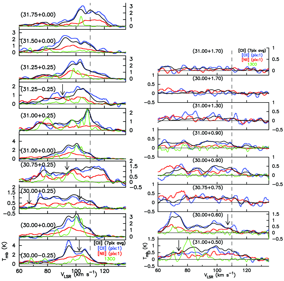
In Figure 5 (left panel) we plot the main beam temperature, $T_{mb}$, for [C ii], [N ii], and ¹³CO(1-0) versus $V_{LSR}$ for ten lines of sight across the Scutum arm ($V_{LSR}\sim$ 60 to 120 km s^-1), from longitude $l$ = 30$\aas@@fstack{\circ}$0 to 31$\aas@@fstack{\circ}$75 and for $b$ within $\pm$0$\aas@@fstack{\circ}$25. In Figure 5 (right panel) we plot these tracers for the eight lines of sight with $b>$ 0$\aas@@fstack{\circ}$25. For each LOS the red and blue lines show [N ii] and the central pixel of [C ii], respectively, while the black line shows the average of the 7 [C ii] pixels. The green lines show the ¹³CO(1-0) profile, which is used as a proxy for the velocity structure of the denser molecular spiral arm gas component. The [C ii] traces both neutral and ionized gas components while [N ii] traces only the ionized gas. The vertical dashed line indicates the tangent velocity as derived from assuming a Galactic rotation model (e.g. Roman-Duval et al. 2009).

In general the [C ii] central pixel and 7-pixel average are similar but there are small differences, as was also shown in the comparison of individual [C ii] pixels in Figure 4. The [C ii] central pixel (blue) and [N ii] (red) profiles represent emissions observed with comparable beams of 14^′′ and 18^′′ sizes, respectively, which allows a direct comparison of their intensities. On the other hand, the [C ii] 7 pixel average profiles (black) correspond to emission smoothed to a larger angular beam, $\sim$ 60^′′ , comparable to the beam size of the ¹³CO ($\sim$45^′′) and H i ($\sim$60^′′) data. To display the velocity structure within the Scutum arm more clearly in Figure 5 we plot only the velocity range of the Scutum arm, V_LSR= 60 – 130 km s^-1.

Comparison of the intensities of the [C ii], $I$([C ii]), central pixel (blue) to [N ii], $I$([N ii]), (red) as a function of $V_{LSR}$ show regions where $I$([C ii]) to $I$([N ii]), is less than 1.5, including some velocities where [N ii] is stronger than [C ii]. Analysis of the predicted contribution of [C ii] from [N ii] regions (see Section 4.2) shows that this ratio can not be less than 1.7 and more typically should be less than 2. The low ratio seen at some velocities in Figure 5 is a result of foreground and/or self-absorption. We have indicated a few of these absorption regions with downward arrows. Evidence for [C ii] absorption, sometimes strong absorption has been noted by Langer et al. (2016) towards other LOS observed in [N ii] and [C ii] with HIFI.

Figure 5: (left) The emission spectra of [C ii] (blue and black), [N ii] (red), and ¹³CO (green) for the ten lines of sight that are within $b=\pm$0$\aas@@fstack{\circ}$25 are plotted as $T_{mb}$ versus velocity. The central [C ii] pixel is plotted in blue and the average of the seven [C ii] pixels is plotted in black. The single and average [C ii] emission profiles are similar but not exactly identical owing to variations in emission across the footprint of the upGREAT array. The black vertical dashed line marks the tangent velocity of the Scutum spiral arm. (right) Figure caption the same as in the left panel for the eight lines of sight with $b>$0$\aas@@fstack{\circ}$25. The downward black arrows mark a few of the clearly evident [C ii] absorption features.

3.2 Longitudinal and latitudinal distribution

The [N ii] and [C ii] emission for the spectra within $|b|<$0$\aas@@fstack{\circ}$25 covering $l$ = 30$\aas@@fstack{\circ}$0 to 31$\aas@@fstack{\circ}$75 in the Scutum tangency, as shown in Figure 5, extend over the same velocity range. In contrast, ¹³CO is present only over portions of the velocity range of the Scutum tangency. The total emission is a blend of several cloud components as can be seen from the complexity in the ¹³CO $(l-v)$ map in Figure 2. While the [N ii] distribution approximately follows that of [C ii], the ratio of $T_{mb}$ of [C ii] to [N ii] varies with $V_{LSR}$. In some lines of sight the [N ii] emission is nearly as strong as [C ii]. This association is seen in other studies of [N ii] and [C ii] and, as noted above, is due in part to [C ii] absorption by low excitation foreground material (Langer et al. 2015).

The latitudinal distribution of the emission shown in Figure 5 (right panel) reveals that ¹³CO is virtually absent for $b>$ 0$\aas@@fstack{\circ}$6 but that [C ii] and [N ii] extend at least up to $b$ = 1$\aas@@fstack{\circ}$3 and perhaps to 1$\aas@@fstack{\circ}$7. Closer to the plane, the emission from [N ii] and [C ii] extend across the entire velocity range of the Scutum tangency, while ¹³CO is restricted to a few velocity components. Taken together, the longitudinal and latitudinal distributions indicate that highly ionized gas, as traced by [N ii] and [C ii], and weakly ionized gas, as traced by a portion of [C ii] are present throughout all layers of the Scutum arm tangency.

3.3 Velocity structure of spiral arm gas components

Figure 6: (top) The spectra for the atomic, molecular, and ionic gas tracers, H i (blue), ¹³CO (green), [C ii] (black), and [N ii] (red), averaged over all LOS within $b=\pm$0$\aas@@fstack{\circ}$25 plotted as main beam temperature, $T_{mb}$, versus $V_{LSR}$. The ionized gas tracers are seen to extend to much higher velocities, corresponding to the innermost leading edge of the Scutum arm, than the molecular gas as traced by ¹³CO. (bottom) An expanded view of the ionized gas emission after subtracting out the [C ii] and [N ii] emission arising from the molecular clouds traced by ¹³CO. The solid green curves represent two of the gaussian components fit to the ¹³CO emission. The dashed green curve is the residual ¹³CO after subtraction. Gaussian profiles were used to fit the [C ii] and [N ii] emission associated with the gas at velocities $<$ 110 km s^-1, while keeping their $V_{LSR}$ at the peak and FWHM the same as the ¹³CO, and only adjusting their peak intensities. Thus what remains for $V_{LSR}\geq$ 110 km s^-1 is the [C ii] and [N ii] excess arising solely from the highly ionized gas with no associated CO.

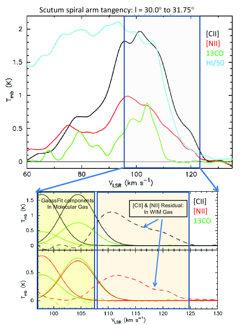
To characterize the overall distribution of gas across the Scutum arm we averaged the spectra from all longitudes ($l$=30$\aas@@fstack{\circ}$0 to 31$\aas@@fstack{\circ}$75) whose lines of sight fall within $b=\pm$0$\aas@@fstack{\circ}$25. This averaging improves the signal-to-noise of the weak WIM emission and avoids biasing the results by observations towards any compact regions. In Figure 6 we plot the resulting $T_{mb}$ from the atomic, molecular, and ionized gas tracers versus $V_{LSR}$. The top panel in Figure 6 compares $T_{mb}$ versus $V_{LSR}$ over the full velocity range of the Scutum tangency (note only the central upGREAT pixel is used so that [C ii] and [N ii] correspond to the same LOS). The shaded rectangle ($V_{LSR}$ = 98 to 125 km s^-1) designates the emission from the inner Scutum arm where the different gas layers are more easily separated. It is clear that the ¹³CO emission does not extend beyond $\sim$110 km s^-1 while [C ii] and [N ii] extend up to at least 125 km s^-1. Thus the [C ii] and [N ii] extend outside the edge of the molecular gas tangency. The [N ii] emission beyond 110 km s^-1 likely arises primarily from the highly ionized gas at the inner edge of the Scutum arm.

To calculate the distribution and properties of the highly ionized gas we need to isolate the velocities over which [N ii] and [C ii] characterize this gas alone versus the emission that comes from PDRs associated with the ¹³CO molecular gas. It has been shown by Velusamy et al. (2015) that the emissions in the gas components trace different gas layers which are well separated in $V_{LSR}$ across the spiral arm tangency. To separate these components we made a multi-gaussian fit to the composite [N ii], the [C ii] central pixel, and ¹³CO spectra in Figure 6 across the velocity range 60 to 130 km s^-1. The high end of this velocity range represents the WIM at the inner edge of the arm and it is highlighted by the shaded box in the upper panel of Figure 6. To separate out any [C ii] or [N ii] contribution in this box that is associated with the molecular gas traced by ¹³CO, we use the gaussian fits to ¹³CO to isolate the molecular components, as follows. We fit the [C ii] and [N ii] emission by adjusting the peak intensity of a set of Gaussian profiles associated with the gas at velocities $<$ 110 km s^-1, keeping their $V_{LSR}$ at the peak and FWHM the same as that for ¹³CO. In the lower panel of Figure 6 we show the two highest velocity ¹³CO gaussian components within the box. We then subtracted out the respective gaussian components for [C ii] and [N ii] and plot the remaining excess in the right hand sub-panel, which represents just the [C ii] and [N ii] contributions from the highly ionized gas at the innermost edge of the Scutum arm.

The strong correlation between the [C ii] and [N ii] emission in the right-subpanel is indicative of [C ii] emission arising from ionized gas with negligible contribution from neutral H i gas (see Section 4.2). The two shaded regions in the lower panel represent schematically the molecular gas (left) and WIM gas (right). The fact that the ¹³CO residual (dashed green line) is negligible shows that the emission in all gas components within the molecular gas layers of the Scutum spiral arm are well accounted for by the two Gaussian profiles (green lines) with linewidths (FWHM) $\sim$7 – 8 km s^-1 and centered at $V_{LSR}$ $\sim$ 98 and 105 km s^-1, respectively. Therefore, we conclude that the [C ii] and [N ii] residuals (black and red profiles, respectively) in the lower panel clearly delineate WIM gas that is well isolated from the molecular spiral arm. Note that the two Gaussian fits to the molecular spiral arm are also consistent with ¹³CO in the ($l$–$V_{LSR}$) map shown in Figure 2.

4 Discussion

Our SOFIA observations provide a rich data set of velocity resolved [C ii] and [N ii] emissions in the Scutum tangency. Our results show widespread clear detections of [C ii] and [N ii] along all LOSs, especially, at velocities $V_{LSR}$ = 60 to 125 km s^-1 and at $|b|$ $<$ 0$\aas@@fstack{\circ}$25. Although weaker at higher latitudes there is detectable emission at least up to $b$ = 1$\aas@@fstack{\circ}$3. The unique combination of [C ii] and [N ii] provides a powerful tool to analyze the ionized gas component in spiral arms and the ability to isolate [C ii] emission in the neutral and ionized gases.

In general the WIM is a highly ionized, low density, $n$(e) $\sim$0.02 to 0.1 cm^-3, high temperature, $T_{k}$= 6000 to 10,000 K gas that fills a 2 - 3 kpc layer around the Galactic midplane (cf. Ferrière 2001; Cox 2005; Haffner et al. 2009). It is estimated to contain about 90% of the ionized gas in the Galaxy and has a filling factor of order 0.2 to 0.4, which may depend on height above the plane. At the midplane the filling factor may be as small as 10%. It has been studied with pulsar dispersion measurements (Cordes & Lazio 2003), H$\alpha$ emission (Haffner et al. 2009, 2016), and nitrogen emission lines in the visible (Reynolds et al. 2001). More recently the WIM has been detected in absorption with [N ii] (Persson et al. 2014). The [C ii] and [N ii] emission lines can also be used to map the WIM, however, the low densities of the WIM make it difficult to detect their emission throughout most of the Galaxy. However, the spiral arm tangencies offer a unique geometry that enables the detection of the WIM in [N ii] and [C ii] because they correspond to regions with a very long path length in a relatively narrow velocity dispersion. The WIM has been detected in [C ii] emission by Velusamy et al. (2012, 2015) along the tangencies of the Perseus, Norma, Scutum, and Crux arms, and they derive higher densities than the interarm WIM. Clearly the WIM in spiral arms is different from that throughout the Galactic disk. In this Section we investigate the extended properties of the warm ionized medium as traced by [C ii] and [N ii] in the tangency region of the Scutum arm.

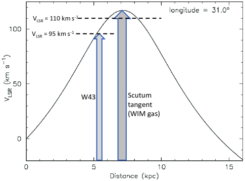
For the analysis and interpretation of the [C ii] and [N ii] emission we adopt a distance of $\sim$7 kpc for the Scutum tangency estimated using the observed $V_{LSR}$ and the Galactic rotation model. In Figure 7 we show the distance–$V_{LSR}$ relationship for the Galactic longitude of the Scutum tangency ($l$= 31$\aas@@fstack{\circ}$0) derived using the rotation curve given by Reid et al. (2014) in their Figure 4 and the Galactic rotation parameters for their Model A5. The rotation velocities in this model for Galactocentric distance, $R_{G}>$ 4 kpc, is quite valid for the location of the Scutum tangency. The WIM component observed at $V_{LSR}>$ 110 km s^-1 is located at the distance of the tangent points, $\sim$7 kpc and extends about $\pm$1 kpc. We note that the distance–$V_{LSR}$ relationship plotted in Figure 7 yields a distance of 5.5 kpc for the star forming region W43 (for $V_{LSR}$ = 95 –110 km s^-1) which is consistent with a distance of 5.5 kpc, obtained from maser parallaxes (Zhang et al. 2014). Thus the Galactic bar-spiral arm interaction region containing W43 appears to be just outside the outer part of the Scutum tangency (see Figure 9).

Figure 7: The distance–$V_{LSR}$ relationship for the Scutum arm tangency at $l$ = 31$\aas@@fstack{\circ}$0 derived using the rotation curve of Reid et al. (2014). It shows that the WIM component of the Scutum tangency is from 6 – 8 kpc, centered at $\sim$7 kpc distance, while the prominent star forming and H ii region, W43, is at about 5.5 kpc.

4.1 Electron density of the Scutum WIM

Nitrogen ions have two fine structure transitions, ³P${}_{1}\rightarrow^{3}$P₀ at 205 $\mu$m and ³P${}_{2}\rightarrow^{3}$P₁ at 122 $\mu$m, and these can be used with an excitation model to calculate the electron density and column density $N$(N⁺). The 122 $\mu$m line needs to be observed from space or a stratospheric balloon due to atmospheric opacity. As we only have one [N ii] transition towards the Scutum tangency observed from SOFIA we cannot determine density $n$(e) and column density $N$(N⁺) independently, however, we can get an idea of the range of $n$(e) using an approach outlined in Langer et al. (2015) that depends on having an estimate of the size of the emission region. For optically thin emission from a uniform region the intensity of the ³P${}_{1}\rightarrow^{3}$P₀ transition can be written (Langer et al. 2015),

$$I_{ion}({\rm[N\,II]})=0.156x_{-4}({\rm N^{+}})L_{pc}n({\rm e})f_{1}(n({\rm e}),T_{k})\,\,{\rm(K\,km\,s^{-1})\,},$$ (1)

where $I_{ion}$([N ii]) is the intensity in K km s^-1, $x_{-4}$(N⁺) is the fractional abundance of N⁺ in units of 10^-4, $L_{pc}$ is the size of the emission region in pc, T_k is the kinetic temperature, and $f_{1}$(n(e),T_k) is the fractional population of the ³P₁ state, which is a function of $T_{k}$ and $n$(e). In the optically thin limit one can solve exactly for the fractional population of the levels as a function of $n$(e) for a given kinetic temperature (Goldsmith et al. 2015). At the high kinetic temperatures associated with highly ionized gas, the kinetic energy of the electrons is orders of magnitude larger than the excitation energies required to populate the ³P₁ and ²P_3/2 states and the solutions are only weakly dependent on T_k through the collisional rate coefficients. For example for the collisional de-excitation rate coefficients calculated by Tayal (2011) the temperature dependence varies from $\sim$ T${}_{k}^{-0.3}$ to T${}_{k}^{-0.5}$ depending on the transition.

Equation 1 can be solved iteratively for $n$(e) as a function of $I_{ion}$([N ii]), using the balance equations for the population of the ${}^{3}P_{2}$ and ${}^{3}P_{1}$ (see Goldsmith et al. 2015), assuming a reasonable value of T_k, and given the size of the emission region and the fractional abundance of N⁺. The critical density (where the collisional de-excitation rate equals the radiative rate) for the ³P₁ level, $n_{cr}(e)$, is $\sim$175 cm^-3, so that at low densities, $n$(e)$<<n_{cr}$(e), Equation 1 can also be solved approximately, within $\pm$15%, using,

$$n(e)=a_{0}\Big{[}\frac{I(\rm{[N\,II]})}{x_{-4}(\rm{N^{+}})L_{pc}}\Big{]}^{\alpha}\,\,{\rm(cm^{-3})}\,,$$ (2)

where, at a characteristic WIM temperature, T_k=8000 K, $a_{0}$= 18.0 and $\alpha$= 0.51 for $n$(e)$\leq$11 cm^-3, and $a_{0}$ =22 and $\alpha$= 0.72, for 11$<$$n$(e)$\leq$ 100 cm^-3.

We consider the average properties of two Galactic zones, one within the plane and the other above the plane. In the plane we average over all LOS within $b=\pm$0$\aas@@fstack{\circ}$25, and above the plane we average all LOS within $b$ =0$\aas@@fstack{\circ}$60 to 0$\aas@@fstack{\circ}$90 (we exclude the LOS at $b$ = 1$\aas@@fstack{\circ}$3 and 1$\aas@@fstack{\circ}$7 because they are too noisy). By using all the data within these two regions we improve the signal to noise and minimize the effects of any localized sources. We adopt a value for the fractional abundance $x$(N⁺) = 1.4$\times$10^-4 (see Section 6.3.2 Goldsmith et al. 2015), appropriate for the Galactic radius, $R_{G}$ = 4 kpc. From the geometry of the Scutum outer arm (see Figure 9 and Reid et al. (2016)) the range $l\sim$ 30^∘ to 32^∘ corresponds to a path length through the tangency $\sim$1$\pm$0.5 kpc, so we adopt $L$ =1 kpc to estimate $n$(e). (In the low density case (see Equation 2) $n$(e) is $\propto$ $L^{-0.5}$ so in choosing $L$=1 kpc the uncertainty in $n$(e) is of order $\pm$25%.) We solved for $n$(e) as a function of $I_{ion}$([N ii]) over the velocity range 110 to 125 km s^-1. We list the intensities and $<$$n$(e)$>$ in Table 1. Typical average densities in the plane, are $<$$n$(e)$>$$\sim$0.9 cm^-3 and above the plane $<$$n$(e)$>$$\sim$ 0.4 cm^-3.

We can also calculate the density of the WIM from [C ii], providing that we have managed to isolate its WIM contribution from other sources (PDRs, CO-dark H₂, H i clouds), using an approach similar to that derived for [N ii]. For $n$(e) less than the critical density for exciting the ²P_3/2 level of C⁺, $n_{cr}$(e) $\sim$45 cm^-3, the electron density is given by (see Velusamy et al. 2012),

$$n(e)=2.92T^{0.18}_{k}\Big{[}\frac{I(\rm{[C\,II]})}{x_{-4}(\rm{C^{+}})L_{pc}}\Big{]}^{0.5}\,\,{\rm(cm^{-3})}\,.$$ (3)

To solve for $n$(e) from [C ii] we adopt $T_{k}$=8000 K (Equation 3 is a very weak function of $T_{k}$) and $x$(C⁺)= 2.9$\times$10^-4 (see Equation 2 in Pineda et al. 2013) appropriate to $R_{G}$ = 4 kpc. We only use the central [C ii] pixel so that we are making a direct comparison of the [N ii] and [C ii] along the same LOS. We find typical values in the plane, $|b|\leq$ 0$\aas@@fstack{\circ}$25, $<$$n$(e)$>\sim$0.8 cm^-3 and above the plane, $\sim$0.3 cm^-3, similar to those derived from [N ii].

Figure 8: (left panels) The integrated intensities of [C ii], [N ii], and ¹³CO (dashed line) over the velocity range 100 to 125 km s^-1 versus latitude. The symbols indicate how many SOFIA LOS were averaged to calculate the emission intensity. The ¹³CO intensity profile is computed using the GRS data cube and we show only high latitude values to demonstrate how sharply it drops to nearly zero by $b$ = 0$\aas@@fstack{\circ}$5. ¹³CO has a much smaller scale height than [C ii] and [N ii]. (right panels) The integrated intensities of [C ii] and [N ii] over the velocity range 110 to 125 km s^-1 versus latitude. There is no measurable ¹³CO in this velocity range, and the [C ii] and [N ii] arise solely from the WIM. The exponential curves correspond to exp(-$(b-\delta b)/b_{0}$ with $\delta b$ = -0$\aas@@fstack{\circ}$05 and $b_{0}$ = 0$\aas@@fstack{\circ}$45.

4.2 [C ii] from the Scutum WIM

As shown in Langer et al. (2016) we can calculate how much [C ii] emission comes from the highly ionized gas, $I_{ion}$([C ii]), in the optically thin limit from the intensity of [N ii], using the following relationship,

$$I_{ion}{\rm([CII])}=0.675\frac{f_{3/2}({\rm C^{+}})}{f_{1}({\rm N^{+}})}\frac{x{\rm(C^{+})}}{x{\rm(N^{+})}}I_{ion}{\rm(NII)}\,\,,$$ (4)

where $f_{i}$ is the fractional population of the corresponding levels. In Equation 4 $f_{3/2}/f_{1}$ is only weakly dependent on density for $n$(e)=10^-3 to 10² cm^-3, and ranges from 1.22 to 1.73, and we adopt $x$(C⁺)/$x$(N⁺) = 2.1.

In Table 1 we give the [C ii] intensity calculated to arise from the WIM, $I_{ion}$([C ii]), corresponding to $V_{LSR}$ =110 – 125 km s^-1, and the fraction of the total observed intensity, $I_{tot}$([C ii]) (the molecular regions are discussed in Section 4.4.2). The [C ii] intensity calculated to arise from the highly ionized gas, $I_{ion}$([C ii]), from just the WIM, $V_{LSR}$ =110 – 125 km s^-1, ranges from 2.0 K km s^-1 out of the plane ($b$=0$\aas@@fstack{\circ}$6 to 0$\aas@@fstack{\circ}$9) to 9.7 K km s^-1 in the plane ($b$=$\pm$0$\aas@@fstack{\circ}$25). In and out of the plane the average fraction $I_{ion}$([C ii])/$I_{tot}$([C ii]) arising from the WIM is $\sim$ 90%. Thus the [C ii] emission from the WIM is a significant fraction of the observed [C ii] intensity towards the WIM, as might be expected from this highly ionized low density medium with very little neutral gas.

If $\sim$90% of the [C ii] emission comes from the highly ionized WIM, then the remaining $\sim$10% probably comes from the H i gas clouds mixed in with the WIM, as there is no molecular gas present. In Figure 6 we see that there is H i emission from 110 to 125 km s^-1. In Table 1 we give the average $I$(H i) in and above the plane, which can readily be converted to an equivalent column density, $N$(C⁺)=1.82$\times$10¹⁸$x$(C⁺)$I$(H i). The corresponding C⁺ column densities in and above the plane are, $N$(C⁺) = 2.6 and 1.3 $\times$10¹⁷ cm^-2, respectively. This column density corresponds to a mean hydrogen density, $<$$n$(H)$>$ = 1.2 and 0.6 cm^-3, respectively. However, because the H i clouds do not fill the LOS, their local density is likely to be much higher. For purposes of estimating their contribution to $I$([C ii]) we assume a typical kinetic temperature $T_{k}$ = 100 K and typical H i cloud densities $n$(H) = 10 – 20 cm^-3. The H i contribution to $I$([C ii]), $I_{{\rm HI}}$([C ii]), even for the larger value of $n$(H)= 20 cm^-3, is $\sim$ 4% in the plane and $\sim$10% out of the plane. This percentage contribution is consistent with the difference between total [C ii] intensity and the $\sim$90% contribution of the WIM to the total [C ii] intensity.

4.3 z-distribution

In principle the scale height of the gas in the disk is a measure of the different forces in the disk, such as gravity and pressure, and thus the energy insertion in the disk. The mass distribution arises from stars, the ISM, and dark matter. The pressure is a result of thermal energy, random motion of clouds, cosmic ray and magnetic pressure, while supernovae and OB-associations provide energy injection that may drive gas into the halo. [C ii] observations with Herschel HIFI made possible the determination of the mean distribution of the gas traced by C⁺. However, because [C ii] traces many different gas components, to get the scale heights of the different ISM components it is necessary to separate out the different scale heights by associating the emission coming from CO, H i, and WIM regions. Velusamy & Langer (2014) analyzed the distribution of all the [C ii] emission detected by the GOT C+ survey as a function of $z$ and found that the average scale height for [C ii] (all gas components) is $\sim$ 170 pc, larger than that for CO, but smaller than that for H i, as might be expected. They found that [C ii] from the WIM and H i combined had a scale height $\sim$330 pc, larger than H i alone. However, with [C ii] alone, they were unable to separate the scale height of the weakly and highly ionized gas. From other studies the highly ionized diffuse gas is known to have a number of components and extend high above the plane.

To determine the $z$–distribution of the ionized gas traced by [C ii] and [N ii] we averaged the spectra for each value of $b$ using observations at adjacent longitudes. This approach reduces the risk that we might have an unusually bright source of emission in the beam and improves the signal-to-noise at the higher latitudes where the emission is weak. To derive the $z$-distribution of the intensity of [C ii] and [N ii] in the WIM we restrict the calculation of intensity to $V_{lsr}$ = 110 to 125 km s^-1 where there is no CO gas (see Figure 6).

In Figure 8 we plot the integrated intensity of [C ii] and [N ii] as a function of $b$, for two different velocity ranges, 100 – 125 km s^-1 (left panel) and 110 – 125 km s^-1 (right panel), where the symbols indicate the number of averaged LOS. The left panel also includes the integrated ¹³CO intensity profile (dashed line) as a function of $b$. The ¹³CO intensity profile is computed using the GRS data cube (Jackson et al. 2006). Note that the CO profile near $b$ = 0$\aas@@fstack{\circ}$0 is uncertain due to complexity in the distribution of strong ¹³CO emission as seen in Figure 2. Nevertheless the high latitude values demonstrate how sharply the ¹³CO emission drops. It is nearly zero by $b$ = 0$\aas@@fstack{\circ}$5, and evidently has a much smaller scale height than [C ii] and [N ii]. In the right panel, where the velocity range corresponds only to WIM gas without any evident molecular component, we find that the data points are roughly consistent with an exponential, $I$=$I_{0}$exp(-$(b-\delta b)/b_{0}$) with a scale height $b_{0}$ = 0$\aas@@fstack{\circ}$45 and offset from plane $\delta b$ = 0$\aas@@fstack{\circ}$05. Within the uncertainty in the measured intensities both [C ii] and [N ii] have similar $z$-scales of $\sim$55 pc assuming a distance of 7 kpc to the tangency. These scale heights do not measure the distribution of the gas density but are measures of the [C ii] and [N ii] emission from the WIM, because their intensities are proportional to $n$(e)², and thus at some point below the sensitvity of the [C ii] and [N ii] surveys.

[C ii] observations with Herschel HIFI made possible the determination of the radial distribution of the gas traced by C⁺. However, because [C ii] traces many different gas components it is necessary to separate out the different scale heights by determining the C⁺ emission coming from CO, H i, and WIM regions. To separate out the different [C ii] sources, Velusamy & Langer (2014) correlated the intensities in 3 km s^-1 wide velocity bins, “spaxels”, in each [C ii] velocity profile with the corresponding spaxel intensities in the ¹²CO, ¹³CO and H i velocity profiles, and found that the [C ii] gaussian scale height for $z$ in the Scutum tangency is smaller than the average value for [C ii] for the disk as a whole. There are a number of possible reasons for the difference. The spaxel analysis was a global average across the disk which had more sensitivity at higher values of $b$ and thus may detect more emission higher in the plane. Second, the Scutum tangency has many active regions of star formation and thus potentially more heating UV. Thus the [C ii] emission in the plane ($|b|\lesssim$ 0$\aas@@fstack{\circ}$5) may be much stronger than the radial average in the plane found by Pineda et al. (2013) and thus skew the fit to a smaller scale height.

Figure 9: A schematic radial cross section view of the spiral arm perpendicular to the LOS to Scutum spiral arm tangency showing the inner to outer edges of the spiral arm (this sketch is not to scale). The molecular gas layer traced by ¹³CO is shown by a thick blue line. Dashed lines show two representative radial velocities and corresponding Galactic locations. The red arc indicates the spiral density wave shock. The location of W43, from the study by Zhang et al. (2014), is marked on the schematic.

4.4 The Source of [N ii] and [C ii] in the Scutum arm

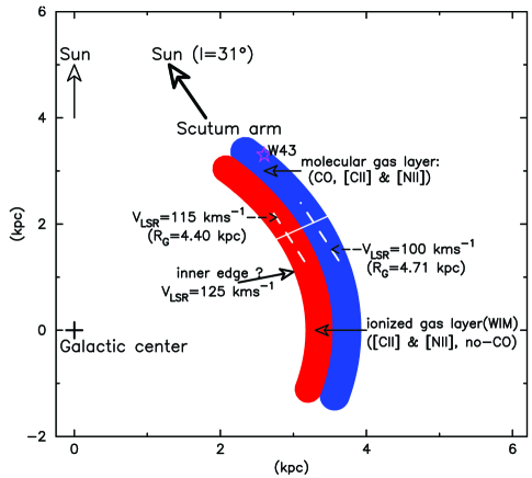
The schematic diagram in Figure 9 illustrates the proposed structure of the gas layers of the Scutum arm as inferred from the observed velocity structure of the gas components traced by [C ii], [N ii], and ¹³CO. In this picture only the WIM is traced by [N ii] and [C ii] at $V_{LSR}>$ 110 km s^-1 and the red curve indicates where a shock might form, while the denser molecular gas layer is traced by ¹³CO at $V_{LSR}<$ 110 km s^-1. We use the unique viewing geometry (as shown in the Figure 9) of the tangency to derive the cross-section view across the spiral arm, from the inner to outer edge, as a function Galacto-centric radial distance (R_G). We use the $V_{LSR}$–R_G relationship assuming pure Galactic rotation, with rotation velocities of 235 km s^-1 and 220 km s^-1 at R_G =4 kpc and R_sun = 8.34 kpc, respectively (c.f. Reid et al. 2014, 2016). Thus the velocity resolved [C ii], [N ii], and ¹³CO spectral data delineate the gas layers of the spiral arm. The low surface brightness [C ii] and [N ii] emission observed at $V_{LSR}>$ 110 km s^-1, which are without associated ¹³CO, is clearly from low density ionized WIM gas located along the inner boundary of the spiral arm. On the other hand the brighter [C ii] and [N ii] emission seen with associated ¹³CO at $V_{LSR}<$ 110 km s^-1 is clearly from the denser ionized gas mixed with the population of dense molecular gas along the mid–layers of the spiral arm. Using the [C ii] emission alone to trace ionized gas, in combination with CO, Velusamy et al. (2015) have shown in the Norma and Perseus tangencies similar evidence for the segregation of the WIM ionized gas layer being displaced inward towards the Galactic center with respect to the dense molecular gas layers of the spiral arm. In the present case of the Scutum tangency, the combination of both [C ii] and [N ii] tracing the ionized gas component supports our prior interpretation of the gas layers distributed from inner to outer edges of the spiral arm as shown in the schematic in Figure 9.

[N ii] is widespread and relatively strong throughout the Scutum spiral arm tangency with typical intensities $I_{ion}$([N ii]) $\sim$ (0.37 – 0.53) $I$([C ii]) (Table 1 column 7). This ratio is much larger than $\sim$ 0.1 to 0.2 found by COBE FIRAS to be typical of the Galactic distribution. The SOFIA $b$ scans show that [N ii] is strongest at the midplane, where the dense molecular cloud tracer ¹³CO is strongest, and decreases with latitude exponentially with a scale height of 0$\aas@@fstack{\circ}$57 and is essentially undetectable beyond 1$\aas@@fstack{\circ}$7. Thus the [N ii] emission observed by COBE FIRAS, with a 7^∘ beam, would have been significantly beam diluted. Here we discuss the conditions and sources of the relatively large electron densities responsible for the [N ii] emission and the large [N ii] to [C ii] ratio in the Scutum arm and by extension in the sparse galactic surveys of [N ii] and [C ii] (Goldsmith et al. 2015; Langer et al. 2016).

4.4.1 WIM component

The electron densities in the WIM derived from [C ii] emission in Velusamy et al. (2012, 2015) and from [N ii] in this paper, are much larger than those characteristic of the Galactic interarm WIM derived using other probes. In the velocity range $V_{LSR}$ = 110 – 125 km s^-1, where there is no evidence of molecular clouds as indicated by the absence of ¹³CO, the [N ii] emission arises almost entirely from the WIM. This result is supported by our estimate that $\sim$90% of the observed [C ii] intensity is associated with the N⁺ gas in this velocity range. The WIM average electron density within $b$ = $\pm$0$\aas@@fstack{\circ}$25 is $\sim$0.4 to 0.9 cm^-3, or about 5 to 20 times larger than the average WIM density, 0.03–0.08 cm^-3 (Haffner et al. 2009), that fills the bulk of the Galactic disk. We interpret this density increase in the inner edge of the arm as due to compression of the interarm WIM in the gravitational potential of the leading edge of the inner spiral arm.

Table 1: Properties of the Scutum arm ionized gas

$b$ range	$V_{LSR}$	$I_{ion}$([N ii])	$<$$n$(e)$>$	$I$([C ii])	$<$$n$(e)$>$	$I$([N ii])/	$I_{ion}$([C ii])	$I_{ion}$([C ii])/	$I$(H i)	$I_{\rm{HI}}$([C ii])a
averaged	km/s	K km/s	cm-3	K km/s	cm-3	I([C ii])	K km/s	$I_{tot}$([C ii])	K km/s	K km/s
-0$\aas@@fstack{\circ}$25 to +0$\aas@@fstack{\circ}$25	110–125	4.05	0.9b	10.8	0.8b	0.37	9.7	0.89	521	0.5
0$\aas@@fstack{\circ}$60 to 0$\aas@@fstack{\circ}$90	110–125	0.82	0.4b	2.2	0.3b	0.38	2.0	0.92	251	0.2
-0$\aas@@fstack{\circ}$25 to +0$\aas@@fstack{\circ}$25	70–110	25.9	40c	49.2	18c	0.53	44.9	$<$0.91d	3700	3.4

a) The [C ii] intensity from the H i gas is calculated assuming $n$(H) = 20 cm^-3. b) $n$(e) for the WIM is derived from $I_{ion}$([N ii]) and $I$([C ii])
assuming $L$ = 1 kpc. c) $n$(e) in the ionized boundary layers is derived from $I_{ion}$([N ii]) and $I$([C ii]) assuming $L$ = 8 pc. d) This value is only an upper limit as there is evidence for foreground and/or self-absorption of [C ii] – see text.

4.4.2 High density ionized gas in the Scutum molecular layer

Unlike the WIM component observed at $V_{LSR}>$ 110 km s^-1 interpreting the strong [N ii] and [C ii] emission features at $V_{LSR}<$ 110 km s^-1 is more challenging as they are mixed with the denser molecular gas component in the spiral arm. These LOSs are located in the W43 complex (W43-south) (see Figure 9), which shows evidence for shocks and compression flows (e.g. Carlhoff et al. 2013) with enhanced star formation. To analyze individual features, we ideally need the densities and/or physical size of the emitting regions. In principle, if we could observe spectrally resolved [N ii] at 122 $\mu$m and 205 $\mu$m we could constrain the density of the ionized gas in the emitting region as a function of $V_{LSR}$. However, the high spectral resolution HIFI instrument on Herschel operated only beyond 157 $\mu$m and Herschel PACS only had a resolving power of $\simeq$1000 at 122 $\mu$m. Presently no heterodyne instrument is available to observe the 122 $\mu$m line.

In their Galactic survey Goldsmith et al. (2015) observed [N ii] with PACS at two lines of sight in the Scutum arm, ($l$,$b$)=(30$\aas@@fstack{\circ}$0,0$\aas@@fstack{\circ}$0) and (31$\aas@@fstack{\circ}$2766,0$\aas@@fstack{\circ}$0). They used the two [N ii] transitions with an excitation model to derive the corresponding electron densities, $n$(e) = 29 and 31 cm^-3 and column densities, $N$(N⁺) = 7.7$\times$10¹⁶ and 11.4 $\times$10¹⁶ cm^-2. They also observed (31$\aas@@fstack{\circ}$2766,0$\aas@@fstack{\circ}$0) in [N ii] 205 $\mu$m with Herschel HIFI and the spectrum shows that nearly all the [N ii] emission was coming from the Scutum arm (Figure 1 in Langer et al. 2016). The [N ii] spectrum of (30$\aas@@fstack{\circ}$0,0$\aas@@fstack{\circ}$0) included here (Figure 5) also shows [N ii] emission throughout the arm. Furthermore, PACS detected [N ii] emission across the 25-pixel array which has a $\sim$45^′′ footprint, corresponding to about 1.5 pc at the distance to the Scutum arm. Thus it is reasonable to surmise that the Scutum arm is an extended source of dense highly ionized gas that coexists with the molecular gas, perhaps as an ionized boundary layer associated with the molecular clouds.

We can estimate the average path length of the emitting region observed with PACS, $L$=$N$(N⁺)$x$(N⁺)/$n$(e), by substituting the values for $n$(e) and $N$(N⁺) from Table 2 in Goldsmith et al. (2015). We find $L$= 6.1 pc and 8.5 pc for the emitting regions in (30$\aas@@fstack{\circ}$0,0$\aas@@fstack{\circ}$0) and (31$\aas@@fstack{\circ}$2766,0$\aas@@fstack{\circ}$0), respectively. However, because the PACS data are spectrally unresolved we cannot separate how much [N ii] 122 $\mu$m emission comes from the WIM tangency and how much from within the molecular arm, which may include dense compact or extended H ii regions or shocked gas. Thus an exact calculation of the density of the different ionized components from an excitation model is not possible without the spectrally resolved 122 $\mu$m line.

Instead, to estimate the average conditions of highly ionized gas in the molecular layers of the arm, we use only the emission in the velocity range where ¹³CO is detected, $V_{LSR}$ = 70 to 110 km s^-1. In Table 1 (row 3) we list the [C ii] and [N ii] intensities for this velocity range. If we assume that most of this emission comes from a region with a total length of 6 – 8 pc, as discussed above, then $n$(e) $\sim$ 40 cm^-3 from $I_{ion}$([N ii]) and $\sim$18 from $I$([C ii]). Thus the densities derived here bracket the values in Goldsmith et al. (2015) and are consistent with the PACS excitation analysis. Such high densities are indicative of H ii regions and the ionized boundary layers (IBL) of dense clouds (Abel et al. 2005; Abel 2006). The multiple velocity features seen in each of the HIFI and GREAT [N ii] spectra show that the total path length of 8 pc will then correspond to about 6 to 10 H ii or IBL components with an average individual depth of $\sim$1 pc. .

Table 1 (row 3) lists the intensity of [C ii] that arises from the [N ii] component, $I_{ion}$([C ii]) = 44.9 K km s^-1, derived using Equation 4. The predicted fractional [C ii] intensity from the highly ionized gas, $I_{ion}$([C ii])/$I_{tot}$([C ii]) = 91%. In addition, as seen in Table 1, the contribution of [C ii] from H i clouds in the plane is $\sim$7%. This result is surprising because it would indicate that very little [C ii] emission comes from PDRs and CO-dark H₂ clouds, which have significant amounts of C⁺ and much higher densities than the H i clouds. However, as seen in Figure 5 and discussed in Section 3.1, there is evidence for multiple [C ii] absorption features and therefore the observed $I_{tot}$([C ii]) is a lower limit to the intrinsic source intensity. Langer et al. (2016) found similarly low [C ii] to [N ii] ratios, sometimes with [N ii] $\geq$ [C ii], towards several of the ten LOS they observed in [C ii] and [N ii] with HIFI. In several components they were able to correct for the absorption and the percentage of emission from the ionized gas ranged from 34% to 58% instead of nearly 100%. Unfortunately the crowding of features along the LOS to the Scutum tangency, as seen in Figures 2 and 5, makes it difficult to correct for the [C ii] absorption using the approach described by Langer et al. (2016). The large fraction of [C ii] arising from [N ii] regions is not just a phenomenon in the Galactic plane as Röllig et al. (2016) observed [C ii] and [N ii] with GREAT in the nearby spiral galaxy IC 342, and showed that 30% – 90% of [C ii] arises from the highly ionized regions traced by [N ii].

That the [N ii] emission is detected throughout the velocity range of the molecular gas, $V_{LSR}$ = 70 to 110 km s^-1, indicates that the ionized boundary layers are distributed throughout the arm. There are two potential sources of the dense highly ionized gas, photoionization by O stars and shock compression of the WIM. In the GRS survey, which includes the Scutum tangency, Anderson et al. (2009) report high, $\sim$ 80%, morphological association between CO and H ii regions, which could account for the wide spread [N ii] associated with ¹³CO in the SOFIA spectra. However, a more likely source of the widespread dense $n$(e) in the [N ii] layers is shock compression as the WIM gas falling into the gravitational potential of the arm, which can accelerate the WIM at the inner gas layer of the spiral arm to a velocity of several km s^-1, much greater than the sound speed in the neutral gas clouds, $\sim$1 km s^-1, resulting in a shock at the interface. This mechanism would also explain the high $n$(e) densities distributed along about 100 LOS throughout the inner galaxy (Goldsmith et al. 2015). In the Scutum arm we might expect to see some shocked gas with enhanced [C ii] and [N ii] emissions due to the proximity of the end of the Galactic bar and spiral arm interaction region. However, the WIM (at $V_{LSR}>$ 110 km s^-1) is fully devoid of CO, that is without any molecular gas, which is more consistent with compression of the interarm WIM by gravitational infall rather than gas streaming from the Galactic bar. Therefore, in our model the ionized boundary layers are continually fueled by the incoming stream of gas.

5 Summary

We report high spectral resolution observations of [C ii] and [N ii] in longitude and latitude across the Scutum spiral arm tangency using upGREAT and GREAT, respectively, on SOFIA. We use these tracers to characterize the highly ionized gas of the WIM in terms of its electron density, the fraction of [C ii] that arises from the highly ionized gas, and the scale height of [C ii] and [N ii] emission. The high spectral resolution observations allow us to separate the [N ii] and [C ii] emission from the WIM from that in the neutral arm. The WIM emission over the inner leading edge of the Scutum arm extends from $V_{LSR}$ = 110 to 125 km s^-1. An analysis of the [N ii] intensity from the WIM indicates an average electron density, $n$(e)$\sim$ 0.9 cm^-3 within $b$ = $\pm$0$\aas@@fstack{\circ}$25, approximately one to two orders of magnitude denser than the interarm WIM. This difference is indicative of compression of the interarm WIM as it flows onto the Scutum arm. The results of combining [N ii] and [C ii] support unambiguously the earlier results of Velusamy et al. (2012, 2015) on the properties of the WIM along spiral arm tangencies based on [C ii] alone. We find that the scale height for the [C ii] and [N ii] emission, $\sim$55 pc, extends beyond that of the molecular gas tracer ¹³CO. A comparison of the [C ii] and [N ii] emission in the WIM shows that a significant fraction, $\sim$90% of the [C ii] arises from the highly ionized gas.

There is widespread, relatively strong [N ii] emission associated with the molecular regions of the Scutum arm, implying that there is highly ionized gas within the arm with $n$(e) $\sim$ 20 – 40 cm^-3 in several thin clumps or layers, totaling about 8 pc in depth. This high density $n$(e) and accompanying [N ii] could be associated with H ii regions distributed throughout the arm, but is most likely the result of shock compression of the WIM, accelerated by the gravitational potential of the Scutum arm. This process may also explain the strong [N ii] emission, high electron densities, and relatively large [N ii] to [C ii] emission observed in recent sparse [N ii] surveys of the inner Galaxy (Goldsmith et al. 2015; Langer et al. 2016). In the molecular arm we can only set an upper limit on the fraction of [C ii] emission that arises from the highly ionized gas traced by [N ii] because of absorption of the [C ii] emission by foreground gas. More extensive maps of spectrally resolved [N ii] and [C ii] of the spiral arms are needed to examine the relatively strong [N ii] emission in the Scutum arm and along many other lines of sight in the Galactic disk.