Entropy production in systems with random transition rates

Abstract

We study the entropy production of a system with a finite number of states connected by random transition rates. The stationary entropy production, driven out of equilibrium both by asymmetric transition rates and by an external probability current, is shown to be composed of two contributions whose exact distributions are calculated in the large system size and close to equilibrium. The first contribution is related to Joule’s law for the heat dissipated in a classical electrical circuit whereas the second one has a Gaussian distribution with an extensive average and a finite variance.

The second law of thermodynamics states that an isolated system relaxing to equilibrium tends to maximize its entropy. However, systems out of equilibrium are ubiquitous in nature, being characterized by a continuous exchange of energy or matter with the environment to maintain a non-equilibrium steady state and, thus, producing entropy Jiang et al. (2004). For this reason, most of the attempts to develop analogous extremal principles valid for non-equilibrium systems ascribe the entropy production to play the leading role Andrieux and Gaspard (2007). Some laws have been proposed Jaynes (1957a, b); Martyushev and Seleznev (2006), stemming from both maximum Dewar (2003) and minimum Prigogine (1955) principles. Nevertheless, the problem remains as one of the greatest challenges of the current statistical physics Goldstein and Lebowitz (2004); Ruelle (1997, 2017); Reis (2014); Gallavotti (2004), partly because of the lack of a universal definition of entropy for systems out of equilibrium Goldstein and Lebowitz (2004); Maes et al. (2000); Seifert (2005). Indeed, the entropy production has been deeply investigated during the last decade in different contexts, yielding to general fluctuation theorems Bustamante et al. (2005); Jarzynski (2008); Seifert (2012) and evidencing universal features that are independent on the system details Pigolotti et al. (2017).

We focus on systems amenable to be described by a continuous time Markovian process, whose dynamics follows a Master Equation (ME) Van Kampen (1992). In this framework, the coupling with the environment results in a set of stochastic transitions between states, with a net positive entropy production. In particular, for a system of $N$ states with corresponding probabilities $p_{i}(t)$, $i=1,\dots,N$, at time $t$ and transition rates $w_{i\rightarrow j}$ ($i,j=1,...N$) satisfying the ME

$$\frac{dp_{i}}{dt}=\sum_{j=1}^{N}(p_{j}w_{j\rightarrow i}-p_{i}w_{i\rightarrow j}),$$ (1)

the entropy production has been argued by Schnakenberg to be given by Schnakenberg (1976):

$$\dot{S}=\sum_{\langle i,j\rangle}(w_{i\rightarrow j}p_{i}-w_{j\rightarrow i}p_{j})\log\frac{w_{i\rightarrow j}p_{i}}{w_{j\rightarrow i}p_{j}}$$ (2)

where the sum is performed over all pairs of states $i,j$ with non-zero transition rates $w_{i\rightarrow j}$ and $w_{j\rightarrow i}$. Note that eq. (2) is always positive and vanishes for systems where detailed balance holds, $p_{i}w_{i\rightarrow j}=p_{j}w_{j\rightarrow i}$, and therefore is a good candidate for the entropy production. Moreover, eq. (2) can be derived from the time derivative of a generalized Gibb’s entropy with an additional term quantifying the entropy flux exchanged with the environment Schnakenberg (1976); Lebowitz and Spohn (1999); Tomé and de Oliveira (2012); Ziener et al. (2015). Its physical meaning and relation with fluctuation-dissipation theorems have been extensively studied in literature Jiu-Li et al. (1984); Maes and Netočnỳ (2003); Bustamante et al. (2005); Tomé and de Oliveira (2012); Zia and Schmittmann (2007); Andrieux and Gaspard (2007); Harris and Schütz (2007); Jarzynski (2008); Seifert (2012).

In his seminal work Schnakenberg (1976), Schnakenberg developed a network theory for systems described by a ME, where the states correspond to nodes connected by links representing the transition rates. In this framework, the entropy production can be related to the topological properties of the underlying network (e.g. loops) via closed formulas, where the circulating currents play the most important role Schnakenberg (1976); Zia and Schmittmann (2006, 2007); Andrieux and Gaspard (2007); Szabó et al. (2010).

In this Letter we propose a random matrix approach to estimate the entropy production in systems described by a ME. The network does not refer to any particular dynamics, but instead is randomly generated owing to constraints (e.g. system size, connectivity, symmetries in the transition rates) that define an ensemble of systems. Random matrices were first introduced by Wigner in the study of the spectrum of heavy nuclei Wigner (1955), and later have found applications in a wide range of fields Crisanti et al. (2012); Allesina and Tang (2012); Sompolinsky et al. (1988). In the same spirit, we employ the framework of random matrices to elucidate the interplay between the system dynamics (encoded in the underlying network topology) and the production of entropy.

We focus on the entropy production of systems at stationarity, $p_{i}(t)=p_{i}^{*}$, for which eq. (2) reduces to Tomé and de Oliveira (2012):

$$\dot{S}^{*}=\sum_{\langle i,j\rangle}(w_{i\rightarrow j}p_{i}^{*}-w_{j\rightarrow i}p_{j}^{*})\log\frac{w_{i\rightarrow j}}{w_{j\rightarrow i}}.$$ (3)

We first consider the simplest case of an open system with symmetric transitions rates, $w_{i\rightarrow j}=w_{j\rightarrow i}=w_{ij}$, which is taken out of equilibrium through the injection of a current of probability $J(t)$ in one of the states. Stationarity is ensured by the ejection of $J(t)$ by another arbitrary state of the system and imposing that $J(t\rightarrow\infty)=J$, i.e. constant at stationarity. The system can be mapped into a network as sketched on the left panel of Fig. 1, and the dynamics is described by the ME:

$$\dot{p}_{i}=\sum_{j=1}^{N}\left(w_{j\rightarrow i}p_{j}-w_{i\rightarrow j}p_{i}\right)+J(t)(\delta_{i,1}-\delta_{i,N})$$ (4)

for $i=1,...N$, where $w_{i\rightarrow j}=w_{ij}$ in the symmetric case and where, without loss of generality, the current enters in node $1$ and exits through node $N$. The external current $J(t)$ can be mimicked by two asymmetric transition rates between nodes $1$ and $N$, $J(t)=p_{N}(t)\omega_{N\rightarrow 1}(t)-p_{1}(t)\omega_{1\rightarrow N}$, where $\omega_{N\rightarrow 1}(t)={(J(t)+\omega_{1\rightarrow N}p_{1}(t))/}{p_{N}(t)}$ becomes constant at stationarity.

Writing $\Delta p=p_{1}-p_{N}$, we define the equivalent transition rate as $w_{\mathrm{eq}}=J/\Delta p>0$, which can be understood as a generalized Ohm’s law for ME systems. Indeed, $w_{\mathrm{eq}}$ is the strength of a symmetric transition rate in a network composed exclusively by nodes $1$ and $N$ that leads to the same $\Delta p$ for a given current $J$, and depends on the topology of the underlying network (see Fig. 1). It is also useful to introduce the parameter $\alpha=p_{1}+p_{N}$, so that $p_{1}=(\alpha+\Delta p)/2$ and $p_{N}=(\alpha-\Delta p)/2$. At equilibrium (i.e. when $J=0$), $p_{i}^{*}=1/N$, and therefore $\alpha=2/N$. In terms of the new variables,

$$\omega_{N\rightarrow 1}=\omega_{1\rightarrow N}+\frac{2J\left(w_{\mathrm{eq}}+\omega_{1\rightarrow N}\right)}{\alpha w_{\mathrm{eq}}-J}.$$ (5)

From eq. (3), it can be seen that internal links do not contribute to the entropy production, and that the only contribution comes from the transition rates between nodes $1$ and $N$:

$$\dot{S}^{*}=J\log\left(\frac{\omega_{N\rightarrow 1}}{\omega_{1\rightarrow N}}\right)\equiv\dot{S}_{\omega}.$$ (6)

We compute the entropy production at stationarity for the system close to equilibrium, i.e. for small values of $J$. Introducing the explicit form of $\omega_{N\rightarrow 1}$ in terms of $J$, eq. (5), and expanding for small values of the current, $J\ll N^{-1}$, we obtain that up to the leading order the entropy production is:

$$\dot{S}^{*}=N\left(\frac{1}{w_{\mathrm{eq}}}+\frac{1}{\omega_{1\rightarrow N}}\right)J^{2}\equiv\dot{S}_{\mathcal{J}},$$ (7)

an expected result since $\dot{S}^{*}\geq 0$ and so the linear contribution in $J$ has to be absent. Eq. (7) consists of two contributions: the first one can be viewed as the entropy production of the system itself, while the second term stems from dissipations in the environment Schnakenberg (1976). The form of $\dot{S}_{\mathcal{J}}$ (eq. (7)) constitutes a fluctuation-dissipation type relation Kubo (1966); Baiesi et al. (2009) and it resembles Joule’s law for the heat dissipated in a classical electrical circuit with equivalent conductance $w_{\mathrm{eq}}/N$, taking also into account the heat dissipated by the battery. The ideal battery corresponds to the limit case $\omega_{1\rightarrow N}=\infty$.

Using the parallelism with the electrical circuit, the stationary state $p_{i}^{*}$ can be retrieved from a variational principle as the one that minimizes the entropy production, with the constraint imposed by the external flux. Such a parallelism also works in the opposite way, as any electrical circuit composed exclusively by multiple resistors can be mapped into a ME system, and its corresponding entropy production turns out to be proportional to the heat dissipation rate (see SI).

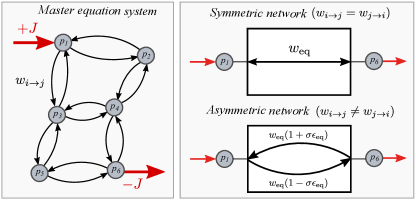
Figure 1: (Left) A master equation (ME) system can be represented by a graph in which nodes correspond to states and links to transition rates between them (sketched here as a 6-nodes network). An external probability current $J$ enters into the system by one of the states and exits from another one to ensure stationarity. We analyze the total entropy production when the system is close to equilibrium. (Right) In symmetric ME systems ($w_{i\rightarrow j}=w_{j\rightarrow i}$), the entropy production can be computed from an equivalent network composed exclusively by the external nodes (the ones coupled to the environment via the external current) linked by a symmetric transition rate of strength $w_{\mathrm{eq}}$. Equivalently, the entropy production of slightly asymmetric networks can be found from an equivalent system composed by the external nodes and two asymmetric links $w_{\mathrm{eq}}(1\pm\sigma\epsilon_{\mathrm{eq}})$. Both $w_{\mathrm{eq}}$ and $\epsilon_{\mathrm{eq}}$ encode the topological structure of the underlying network.

Before moving to the more general case of non-symmetric transition rates and also for later comparison reasons we have checked numerically the validity of eq. (7) on randomly generated ME systems of size $N$ and connectivity $K$ (defined as the fraction of non-directed connections respect to the $N(N-1)/2$ links in the fully-connected case). In the symmetric case, each non-null entry of $w_{i\rightarrow j}$ is taken from a Gaussian distribution with average $w$ and standard deviation $w\sigma$, with the constraint that $w_{i\rightarrow j}=w_{j\rightarrow i}$ for each pair of links. We numerically integrate the corresponding ME and compute the entropy production at stationarity. The result is compared with eq. (7), where all the dependency on the network topology in eq. (7) is encapsulated in the parameter $w_{\mathrm{eq}}$. Results are shown in Top panel of Fig. 2 (in log-log scale), evidencing that eq. (7) perfectly works for a wide range of values of $J$.

Now we want to generalize the simple result given by eq. (7) to networks generated as in the symmetric case but taking $w_{i\rightarrow j}$ and $w_{j\rightarrow i}$ as independent random variables. For each topology, $w_{\mathrm{eq}}$ is simply estimated taking $w_{i\rightarrow j}=w$. Then, we compute the entropy production of each network in the presence of a probability current $J$, and compare its value with the one given by $\dot{S}_{\mathcal{J}}$. Results are presented in the Bottom panel of Fig. 2 for different values of the heterogeneity $\sigma$; the prediction given by eq. (7) fails in the limit of small flux, as detailed balance does not holds for a general asymmetric network, and therefore $\dot{S}\neq 0$ when $J\rightarrow 0$.

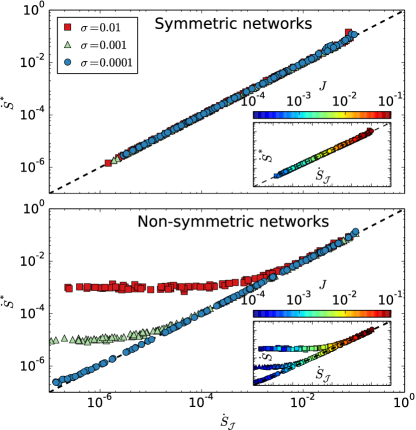
Figure 2: Entropy production of ME systems represented by random (Erdos-Renyi) networks, compared to the theoretical prediction given by Eq. (7). Transition rates $w_{i\rightarrow j}$ are randomly generated from a Gaussian distribution with mean $w=1$ and standard deviation $w\sigma$. Each dataset is composed by $100$ realizations of networks of size $N=25$, fixing the parameter $\omega_{1\rightarrow N}=10$. The external flux $J$ is a random variable, being $\log_{10}J$ uniformly distributed in $[-4,-1]$ (so that $J\in[10^{-4},10^{-1}]$). All plots are in log-log scale. (Top panel) Symmetric networks, for which $w_{i\rightarrow j}=w_{j\rightarrow i}$ for each pair of links. The connectivity $K$ is a uniform random variable in $K\in[0.25,1]$. (Bottom Panel) - Non-symmetric networks: we remove the symmetric constraint, and therefore $w_{i\rightarrow j}\neq w_{j\rightarrow i}$ in general. In this case, we have fixed the connectivity $K=0.5$. In both panels, insets represent the same corresponding points but using a color scale for the external probability flux $J$. Similar results can be obtained for other network topologies different from the Erdos-Renyi (Eq. (7) is valid in general).

Deviations from eq. (7) due to asymmetries in the network can be described within a perturbative framework when the system is close to equilibrium. We focus on ensembles of random Erdos-Renyi topologies of connectivity $K$ for which the non-null elements of $w_{i\rightarrow j}$ are independent Gaussian random variables of mean $w$ and standard deviation $w\sigma$. Erdos-Renyi topologies are good proxies for networks with limited connectivity for which the property of small world holds Newman (2003). Notice that, in the (rather general) case of a system composed by $n$ elementary units, each of them taking $m$ possible values, the total number of states is $N=n^{m}$. If the dynamics allows that each unit can change its value once at a time, the system can pass from one state to another through, roughly, $n$ individual steps. This leads to a typical path distance of the order of $n=\log_{m}(N)$, which is actually the small world condition Newman (2003). Introducing the adjacency matrix $A_{ij}=\Theta[w_{i\rightarrow j}]$ ($\Theta$ is the Heaviside step function with $\Theta(0)=0$), we can write $w_{i\rightarrow j}=wA_{ij}(1+\sigma\epsilon_{ij})$ in terms of independent Gaussian variables $\epsilon_{ij}$ of zero mean and unit variance.

The entropy production given by eq. (3) can be split into two contributions,

$$\dot{S}^{*}=\dot{S}_{\mathrm{int}}+\dot{S}_{\omega},$$ (8)

where $\dot{S}_{\mathrm{int}}$ is the one given by internal links in the network and $\dot{S}_{\omega}$ the one given by the external links connecting nodes $1$ and $N$, eq. (6). Formally, such a separation can be done if we do not allow the presence of internal links $w_{1\rightarrow N}$ and $w_{N\rightarrow 1}$, although whether considering them or not does not significantly change the value of the entropy production in large networks.

We want to show that close to equilibrium, $J,\sigma\ll N^{-1}$, the entropy production, $\dot{S}^{*}$, differs from the corresponding one in absence of asymmetry, $\dot{S}_{\mathcal{J}}$, as given by eq.(7), by a gaussian random variable of mean $(KN-2-K+\mathcal{O}(1/N))w\sigma^{2}$ and variance $4Kw^{2}\sigma^{4}+\mathcal{O}(1/N)$. To show that we write the stationary state as $p_{i}^{*}\simeq\left(1+\sigma q_{i}+Jr_{i}\right)/N$; the normalization constraint implies that $\sum_{i}q_{i}=\sum_{i}r_{i}=0$. Then, we expand the entropy production in terms of $\sigma$ and $J$, neglecting contributions of order higher than $\sigma JN^{2}$, $\sigma^{2}N^{2}$ and $J^{2}N^{2}$. Defining the antisymmetric matrix $D_{ij}=\epsilon_{ij}-\epsilon_{ji}$ (whose entries are Gaussian variables with zero mean and standard deviation $\sqrt{2}$), the first order contributions to $\dot{S}_{\mathrm{int}}$ are:

$$\frac{\dot{S}_{\mathrm{int}}}{w\sigma^{2}}=\frac{1}{N}\sum_{\langle i,j\rangle}A_{ij}\left(D_{ij}^{2}+D_{ij}\left(q_{i}+\frac{J}{\sigma}r_{i}\right)\right).$$ (9)

For large $N$, the first term of the r.h.s. of eq. (9), becomes a Gaussian random variable of mean $K(N-1)$ and standard deviation $2\sqrt{K}$ by means of the central limit theorem (see SI). Remarkably, this term is positive and scales linearly with the system size $N$. The second and third terms in eq. (9) require to solve the ME close to equilibrium to obtain the values of $q_{i}$ and $r_{i}$. Up to first order in $N$, we find that $q_{i}\simeq-\frac{1}{KN}\sum_{j}A_{ij}D_{ij}$ (see SI). Such a dependency is meaningful: if in a node $i$, most of $D_{ij}=(w_{i\rightarrow j}-w_{j\rightarrow i})/w>0$ (resp. $<0$), an outgoing (incoming) flux is expected between node $i$ and its neighbors, and therefore $p_{i}^{*}<1/N$ ($>1/N$). Introduced in eq. (9), the second term gives a Gaussian random contribution to $\dot{S}_{\mathrm{int}}$ with mean $-2$ and standard deviation $\sqrt{8/N}$ (see SI). Equivalently, solving the ME we find that, up to first order in $N$, $r_{i}\simeq(\delta_{i1}-\delta_{iN})/(wK)$ (see SI), evidencing the major role of the external nodes. This term gives another Gaussian contribution to $\dot{S}_{\mathrm{int}}$ which has zero mean and standard deviation $(2/\sqrt{KN})J/\sigma$ (see SI). Assembling all the terms together, the leading contributions give that $\dot{S}_{\mathrm{int}}$ is normally distributed with mean and variance given by:

$$\langle\dot{S}_{\mathrm{int}}\rangle=\left(KN-(2+K)\right)w\sigma^{2}+\mathcal{O}(1/N)$$ (10)

$$\langle(\dot{S}_{\mathrm{int}})^{2}\rangle-\langle\dot{S}_{\mathrm{int}}\rangle^{2}=4Kw^{2}\sigma^{4}+\mathcal{O}(1/N)$$ (11)

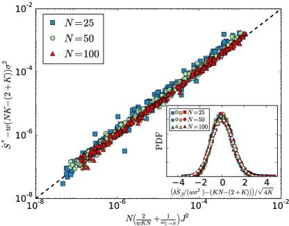
Figure 3: Deviations from eq. (7) follow generic scaling relations. The relation between $\dot{S}^{*}$ and $J$ for networks generated with different $N$, $K$, $J$ and $\sigma$ can be enlightened plotting $\dot{S}^{*}-\langle\delta\dot{S}_{\mathcal{J}}\rangle$ against $\langle\dot{S}_{\mathcal{J}}\rangle$. All datasets collapse into the straight line $y=x$ (with deviations around). We have generated 250 networks for each system size with a random connectivity uniformly distributed in $K\in[0.25,1]$ and a external flux $J$ such that $\log_{10}J$ is a uniform random variable in $[-4,-1]$ ($J\in[10^{-4},10^{-1}]$); the heterogeneity has been taken $\sigma=J$ for each realization (this ensures that the current and heterogeneity contributions to the entropy production are of the same order and therefore both have to be considered). (Inset) We collapse the PDFs of $\delta\dot{S}_{\mathcal{J}}$ by subtracting the contribution given by Joule’s law, eq. (7), and the mean $w(KN-(2+K))\sigma^{2}$, and dividing by the standard deviation $w\sqrt{4K}\sigma^{2}$ (blue, green, yellow and red points correspond to $K=0.25,0.5,0.75$ and $1$, respectively). The corresponding $w_{\mathrm{eq}}$ is computed setting $w_{i\rightarrow j}=w$ for each network topology. All histograms collapse into a Gaussian distribution of zero mean and unit variance (dashed line). We have generated $10^{4}$ independent realizations for each set of parameters, setting $J=\sigma=10^{-3}$. We have set $\omega_{1\rightarrow N}=10$ in both panels.

On the other hand, the term $\dot{S}_{\omega}$ can be computed in terms of a generalized Ohm’s law for non-symmetric networks close to equilibrium, $\Delta p=J/w_{\mathrm{eq}}+\sigma\epsilon_{\mathrm{eq}}$, where $1/w_{\mathrm{eq}}=(r_{1}-r_{N})/N$ and $\epsilon_{\mathrm{eq}}=(q_{1}-q_{N})/N$ is a network parameter accounting for the asymmetry-induced unbalance between nodes $1$ and $N$. More precisely, $\epsilon_{\mathrm{eq}}$ represents the asymmetry of an equivalent network composed exclusively by nodes $1$ and $N$ with the same $\Delta p$ and $(w_{N\rightarrow 1}-w_{1\rightarrow N})/(w_{N\rightarrow 1}+w_{1\rightarrow N})=\sigma\epsilon_{\mathrm{eq}}$ (see Fig. 1). Notice that $w_{\mathrm{eq}}$ and $\epsilon_{\mathrm{eq}}$ exclusively depends on the network structure. In terms of these parameters, the leading contributions to $\dot{S}_{\omega}$ are:

$$\dot{S}_{\omega}(\sigma)=\dot{S}_{\mathcal{J}}+N\epsilon_{\mathrm{eq}}\sigma J,$$ (12)

where $\dot{S}_{\mathcal{J}}$ is defined in eq. (7). Deviations from eq. (7), $\delta\dot{S}_{\mathcal{J}}=\dot{S}^{*}-\dot{S}_{\mathcal{J}}$ are given by $\delta\dot{S}_{\mathcal{J}}=\dot{S}_{\mathrm{int}}+N\epsilon_{\mathrm{eq}}\sigma J$. For large networks we found that $\epsilon_{\mathrm{eq}}$ is normally distributed, $\epsilon_{\mathrm{eq}}\sim\mathcal{N}\left(0,2/\sqrt{KN^{3}}\right)$ (see SI). Consequently, deviations from eq. (7) are essentially given by $\delta\dot{S}_{\mathcal{J}}\approx\dot{S}_{\mathrm{int}}$, which is our main result.

The relation between $S^{*}$ and $J$ can be enlightened representing $\dot{S}^{*}-\langle\delta\dot{S}_{\mathcal{J}}\rangle=\dot{S}^{*}-(NK-(2+K))w\sigma^{2}$ against $\langle\dot{S}_{\mathcal{J}}\rangle=N\left(\langle w_{\mathrm{eq}}^{-1}\rangle+\omega_{1\rightarrow N}^{-1}\right)J^{2}$. We can compute the distribution of $w_{\mathrm{eq}}$ for an ensemble of random networks of size $N$ and connectivity $K$; interestingly, this problem is equivalent to computing the equivalent conductance of an electrical circuit in which resistors are randomly connected. $P(w_{\mathrm{eq}})$ becomes a Gaussian distribution with mean $NKw/2$ and standard deviation $w\sqrt{NK(1-K)/8}$ for large networks (see SI), becoming narrower when $N$ increases (relatively to its mean). Therefore, we can use the approximation $\langle w^{-1}_{\mathrm{eq}}\rangle\sim eq2/(NKw)$ (we refer to the SI for a more formal derivation). Pairs of $(S^{*},J)$ are represented with this procedure in the main panel of Fig. 3, evidencing that the entropy production of non-symmetric ME systems of different sizes $N$, connectivity $K$, heterogeneity $\sigma$ and external current $J$, all collapse around the straight line $y=x$, with deviations around decreasing for larger systems.

Finally, we check numerically that deviations from eq. (7) follow the scaling relations given by equations (10) and (11). Subtracting the mean and dividing by the standard deviation, all the histograms collapse into the Gaussian distribution with zero mean and unit variance, as depicted in the inset of Fig. 3.

Summarizing, in this Letter we have employed the network theory proposed by Schnakenberg to analyse the entropy production of systems out of equilibrium from a random matrix perspective. We have obtained general scaling relations for the entropy production of network ensembles representing a set of systems and dynamics, and we have identified the topological parameters ($w_{\mathrm{eq}}$ and $\epsilon_{\mathrm{eq}}$) that play the most important role.

Our framework provides a null-model on which compare the entropy production of specific systems and dynamics. In particular, some biological systems seem to have evolved in order to dissipate energy and produce entropy at the minimum or maximum possible rate Martyushev and Seleznev (2006); Kleidon et al. (2010). It could be interesting to analyse the topological features of real dynamics (in particular the values of $w_{\mathrm{eq}}$ and $\epsilon_{\mathrm{eq}}$) with what we have obtained for random networks, which have not been obtained through optimization/evolution processes.

Finally, our results has been derived for small world-like networks with an homogeneous degree distribution of finite variance. Interesting generalizations include cases where the degree distribution has not a finite variance, e.g. scale free-networks Barabási and Albert (1999), strong asymmetric transition rates and transition rates between different pairs of states with non-trivial correlations.

We thank S. Suweis and S. Azaele for useful discussions and suggestions.

Supplementary Information for
Entropy production in systems with random transition rates
D. M. Busiello, J. Hidalgo and A. Maritan

Appendix A Mapping: from an electrical circuit into a ME system

Let us consider a circuit $\mathcal{C}$ composed of $N$ nodes connected by multiple resistors, with conductances equal to $c_{ij}$. When a difference of potential $\Delta V=V_{1}-V_{N}$ is applied between nodes $1$ and $N$, the potential at each node $i$, $V_{i}$, is given by Kirchoff’s law, which ensures the minimization of the heat dissipation:

$$\dot{Q}=\sum_{\langle i,j\rangle}c_{ij}(V_{i}-V_{j})^{2}$$ (13)

where the sum is performed over all pairs of nodes $i$, $j$. One can then build a fictitious dynamics for the potentials, whose stationary state corresponds to the physical state of $\mathcal{C}$. To proceed, we fix $V_{1}$ and $V_{N}$ (with $V_{1}-V_{N}=\Delta V$), and consider the following dynamics for nodes $i=2,...,N-1$:

$$\tau\dot{V}_{i}(t)=-\frac{\partial\dot{Q}}{\partial V_{i}}=\sum_{j=1}^{N}c_{ij}\left(V_{j}-V_{i}\right).$$ (14)

An arbitrary time scale $\tau$ can be introduced without changing the stationary state. Notice that eq. (14) leads to the state which minimizes $\dot{Q}$, as $\ddot{Q}(t)=\sum_{i}\frac{\partial\dot{Q}}{\partial V_{i}}\dot{V}_{i}=-2\tau\sum_{i}\dot{V}_{i}^{2}<0$. Let us notice that, despite its analogy, eq. (14) is not a master equation, since $\sum_{i=1}^{N}\dot{V}_{i}(t)\neq 0$ for arbitrary $t$, and therefore normalization is not conserved. However, one can relax the constraint on nodes $1$ and $N$ to be obeyed only at stationarity. Defining the normalized potentials, $v_{i}=V_{i}/\sum_{i}V_{i}=V_{i}/V_{T}$ and introducing the new parameters $c_{1\rightarrow N}$ and $c_{N\rightarrow 1}$ ($c_{1\rightarrow N}\neq c_{N\rightarrow 1}$ in general), we study the following ME dynamics:

$$\tau\dot{v}_{i}(t)=\sum_{j}c_{ij}(v_{j}-v_{i})+\left(c_{N\rightarrow 1}v_{N}-c_{1\rightarrow N}v_{1}\right)(\delta_{i,1}-\delta_{i,N})$$ (15)

for $i=1,...,N$, where $c_{N\rightarrow 1}$ and $c_{1\rightarrow N}$ have to be chosen to ensure $v_{1}-v_{N}=\Delta V/V_{T}$ at stationarity. Notice that $\sum_{i=1}^{N}\dot{v}_{i}=0$ for arbitrary $t$ in eq. (15), which has an equivalent form to eq. (4). In addition, it leads to the state minimizing the heat dissipated by the circuit. Without loss of generality we can fix $\tau=1$.

The normalized current, $J=c_{N\rightarrow 1}v_{N}-c_{1\rightarrow N}v_{1}=c_{\mathrm{eq}}\Delta V/V_{T}=I/V_{T}$, where $c_{\mathrm{eq}}$ is the conductance of the equivalent circuit formed by one single resistor and $I$ is the supplied electrical current. For small values of the external current, Schnakenberg’s entropy production at stationarity is given by eq. (7):

$$\dot{S}^{*}=N\left(\frac{1}{c_{\mathrm{eq}}}+\frac{1}{c_{1\rightarrow N}}\right)J^{2},$$ (16)

which corresponds to Eq. (7) of the main text with $c_{\mathrm{eq}}=w_{\mathrm{eq}}$ and $c_{1\rightarrow N}=\omega_{1\rightarrow N}$. Written in terms of the heat dissipated by the circuit, $\dot{Q}=I^{2}/c_{\mathrm{eq}}$, the entropy production of the associated ME dynamics is:

$$\dot{S}^{*}=\frac{N}{V_{T}^{2}}\left(1+\frac{c_{\mathrm{eq}}}{c_{1\rightarrow N}}\right)\dot{Q}.$$ (17)

Its important to note that the relation given by eq. (17) is determined up to the specific choice of parameters $V_{T}$ and $c_{1\rightarrow N}$, as this is an intrinsic ambiguity of the mapping. Furthermore, there is a dissipation contribution coming from the battery, which vanishes in the the limit of a “perfect” battery, $c_{1\rightarrow N}\rightarrow\infty$.

Appendix B Calculation of $\dot{S}_{\mathrm{int}}$

Writing the transition rates $w_{i\rightarrow j}$ in terms of independent Gaussian variables $\epsilon_{ij}$ of zero mean and unit variance, $w_{i\rightarrow j}=A_{ij}w(1+\sigma\epsilon_{ij})$ (with $A_{ij}=\Theta[w_{i\rightarrow j}]$) and introducing $p_{i}^{*}=(1+\sigma q_{i}+Jr_{i})/N$ in eq. (3), we obtain:

$$\dot{S}_{\mathrm{int}}=\sum_{\langle i,j\rangle}A_{ij}w\left((1+\sigma\epsilon_{ij})\left(\frac{1}{N}\left(1+\sigma q_{i}+Jr_{i}\right)\right)-(1+\sigma\epsilon_{ji})\left(\frac{1}{N}\left(1+\sigma q_{j}+Jr_{j}\right)\right)\right)\log\left(\frac{1+\sigma\epsilon_{ij}}{1+\sigma\epsilon_{ji}}\right).$$ (18)

Close to equilibrium ($\sigma\ll N^{-1},J\ll N^{-1}$), the leading contributions are:

$$\dot{S}_{\mathrm{int}}^{1} = \frac{w\sigma^{2}}{N}\sum_{\langle i,j\rangle}A_{ij}D_{ij}^{2}$$ (19)

$$\dot{S}_{\mathrm{int}}^{2} = \frac{w\sigma^{2}}{N}\sum_{\langle i,j\rangle}A_{ij}D_{ij}(q_{i}-q_{j})=\frac{w\sigma^{2}}{N}\sum_{i,j}A_{ij}D_{ij}q_{i}$$ (20)

$$\dot{S}_{\mathrm{int}}^{3} = \frac{w\sigma J}{N}\sum_{\langle i,j\rangle}A_{ij}D_{ij}(r_{i}-r_{j})=\frac{w\sigma J}{N}\sum_{i,j}A_{ij}D_{ij}r_{i},$$ (21)

where $D_{ij}=\epsilon_{ij}-\epsilon_{ji}$. In the next section we compute each term separately, and we show that the major contribution is given by $\dot{S}_{\mathrm{int}}^{1}$, whereas the second and the third term can be neglected for large network sizes. For convenience, we will call $\mathcal{N}(a,b)$ the Gaussian distribution with mean $a$ and standard deviation $b$.

It is worth mentioning that, in our calculations, we do not distinguish the cases in which the external nodes are or not connected also by internal nodes ($A_{1N}=0$ and $1$ respectively), as this constitutes a minor contribution for the total entropy production.

B.1 Calculation of $\dot{S}_{\mathrm{int}}^{1}$

For each pair of links $i$ and $j$, $D_{ij}$ is an independent random variable of zero mean and standard deviation $\sqrt{2}$. Therefore, $D_{ij}^{2}$ is distributed as a chi-square distribution whose mean and variance can be easily calculated:

$$\langle D_{ij}^{2}\rangle = 2$$ (22)

$$\langle(D_{ij}^{2}-\langle D_{ij}^{2}\rangle)^{2}\rangle = \langle D_{ij}^{4}\rangle-\langle D_{ij}^{2}\rangle^{2}=2\langle D_{ij}^{2}\rangle^{2}=8.$$ (23)

Eq. (19) involves the sum of $KN(N-1)/2$ independent variaeq.bles of this type. When $N$ is large, by means of the Central Limit Theorem, we obtain that $\dot{S}_{\mathrm{int}}^{1}$ follows a normal distribution:

$$P\left(\frac{\dot{S}_{\mathrm{int}}^{1}}{w\sigma^{2}}\right)=\mathcal{N}\left(K(N-1),2\sqrt{K\left(1-\frac{1}{N}\right)}\right)\simeq\mathcal{N}(K(N-1),2\sqrt{K}).$$ (24)

B.2 Calculation of $\dot{S}_{\mathrm{int}}^{2}$

In the absence of external flux ($J=0$) and for small asymmetry $\sigma$, the stationary state can be written as $p_{i}^{*}=\frac{1}{N}(1+\sigma q_{i})$. The values of $q_{i}$ can be retrieved solving the master equation at stationarity:

$$0=\sum_{j}A_{ij}w\left((1+\sigma\epsilon_{ji})\left(\frac{1}{N}\left(1+\sigma q_{j}\right)\right)-(1+\sigma\epsilon_{ij})\left(\frac{1}{N}\left(1+\sigma q_{i}\right)\right)\right),$$ (25)

that, up to first order in $\sigma$, leads to the implicit solution:

$$q_{i}=\frac{1}{k_{i}}\left(-\sum_{j}A_{ij}D_{ij}+\sum_{j}A_{ij}q_{j}\right),$$ (26)

where $k_{i}=\sum_{j}A_{ij}$ is the number of nodes connected to node $i$. For convenience, we introduce self-interactions ($A_{ii}=1$), as this choice does not change the dynamics in the master equation and leads to simpler expressions in our notation. In the fully connected network ($A_{ij}=1$), the second term on the r.h.s. of eq. (26) vanishes (as $\sum_{j}q_{j}=0$), leading to the closed form $q_{i}=-\frac{1}{N}\sum_{j}D_{ij}$. This result is rather intuitive: if, for instance, the average rate of the outgoing links in a node $i$ is greater than the ingoing one (the same argument applies in the opposite case) $\sum_{j}\epsilon_{ij}>\sum_{j}\epsilon_{ji}\Longrightarrow\sum_{ij}D_{ij}>0$, there is a net outgoing flux to its neighbors and therefore $q_{i}<0$, or equivalently, $p_{i}^{*}<1/N$.

For a general connectivity $K$, we can neglect the implicit term in eq. (26), leading to:

$$q_{i}\simeq-\frac{1}{k_{i}}\sum_{j}A_{ij}D_{ij},$$ (27)

which turns out to be a rather accurate approximation, especially for large $N$, as illustrated Fig. 4 (left panel). Corrections to this formula are of $\mathcal{O}(N^{-1})$ (see Fig 4, right panel), and therefore can be neglected for large system sizes. Indeed, notice that the approximate form of eq. (27) does not satisfy the constraint $\sum_{i}p_{i}^{*}=1+\sigma\sum_{i}q_{i}/N=1$ in general, but the error vanishes when $N\rightarrow\infty$.

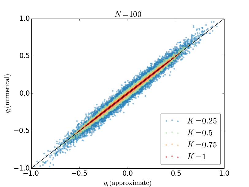
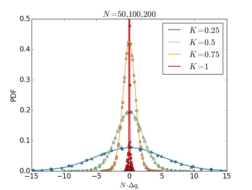
Figure 4: We generate random Erdos-Renyi topologies of mean connectivity $K$ and size $N$, where each link $w_{i\rightarrow j}$ is an independent Gaussian variable of mean $w$ and standard deviation $\sigma w$. We set $w=1$ and $\sigma=10^{-2}$. In the absence of external flux ($J=0$), we integrate numerically the associated master equation until stationarity, and calculate $q_{i}=(Np_{i}^{*}-1)/\sigma$. (Left panel) We compare the numerical value of $q_{i}$ with the one given by the approximation of eq. (27), for all the nodes in the network and for $10^{3}$ randomly generated networks. Network size has been set to $N=100$. (Right panel) PDF of the error made in eq. (27), rescaled with the system size $N$, for $N=50$ (circles), $N=100$ (solid line) and $N=200$ (triangles), for different connectivities with the same colorcode as on the left panel. For each connectivity, the PDFs of the rescaled error $N\Delta q_{i}$ collapse into a single curve, illustrating that the error $\Delta q_{i}=\mathcal{O}(N^{-1})$.

We can introduce eq. (27) into eq. (20), obtaining:

$$\dot{S}_{\mathrm{int}}^{2}=-\frac{w\sigma^{2}}{N}\sum_{i}\frac{1}{k_{i}}\left(\sum_{j}A_{ij}D_{ij}\right)^{2}.$$ (28)

For each $i$, $\sum_{j}A_{ij}D_{ij}$ is a Gaussian random variable with zero mean and variance $2(k_{i}-1)$, and therefore $(\sum_{j}A_{ij}D_{ij})^{2}/k_{i}$ follows a chi-squared distribution of mean $2(1-k_{i}^{-1})\simeq 2$ and variance $8(1-k_{i}^{-1})^{2}\simeq 8$, as $k_{i}^{-1}$ can be neglected for large network sizes. Finally, we have to sum over nodes $i$; in principle, one cannot apply straightforwardly the Central Limit theorem, as the elements of the sum present correlations. Think, for instance, in the simple case of a triangle network, where one has to calculate $(D_{12}+D_{13})^{2}+(D_{21}+D_{23})^{2}+(D_{31}+D_{32})^{2}$, where $D_{ij}=-D_{ji}$. However, the number of correlated elements in the sum becomes negligible with the number of uncorrelated ones for large system sizes, so one can simply neglect such a correlation. After these approximations, we find:

$$P\left(\frac{\dot{S}_{\mathrm{int}}^{2}}{w\sigma^{2}}\right)\simeq\mathcal{N}\left(-2,\sqrt{\frac{8}{N}}\right).$$ (29)

Notice that $\langle\dot{S}_{\mathrm{int}}^{2}\rangle$ is independent of $N$, whereas $\langle\dot{S}_{\mathrm{int}}^{1}\rangle$ grows linearly with $N$ (eq. (24)). Therefore, the former can be neglected respect to the latter.

B.3 Calculation of $\dot{S}_{\mathrm{int}}^{3}$

We compute $\dot{S}_{\mathrm{int}}^{3}$ following a similar approach as for $\dot{S}_{\mathrm{int}}^{2}$. In the absence of asymmetry, $\sigma=0$, and for small external flux $J$, the stationary state is written as $p_{i}^{*}=\frac{1}{N}\left(1+Jr_{i}\right)$. To find $r_{i}$, we solve the master equation at stationarity:

$$0=\sum_{j}A_{ij}\frac{w}{N}\left(r_{j}-r_{i}\right)J+J\left(\delta_{i1}-\delta_{iN}\right)$$ (30)

whose solution is:

$$r_{i}=\frac{N}{wk_{i}}\left(\delta_{i1}-\delta_{iN}+\frac{w}{N}\sum_{j}A_{ij}r_{j}\right).$$ (31)

In the fully connected network ($A_{ij}=1$), the second term on the r.h.s. vanishes (since $\sum_{j}r_{j}=0$), leading to $r_{i}=(\delta_{i1}-\delta_{iN})/w$. This means that all nodes have equal probabilities except for the $1$st and $N$th, that present a small unbalance $p_{1}-p_{N}=2J/(Nw)$. Consequently, $w_{eq}=Nw/2$ in the fully connected network). As we did for the calculation of $\dot{S}_{\mathrm{int}}^{2}$, we can use this solution as an approximation for a general connectivity $K$,

$$r_{i}\simeq\frac{N}{wk_{i}}\left(\delta_{i1}-\delta_{iN}\right).$$ (32)

As for the case of $q_{i}$, the approximate form above does not satisfy the constraint $\sum_{i}p_{i}^{*}=1+J\sum_{i}r_{i}/N=1$ in general, but the error made vanishes when $N\rightarrow\infty$. Plugging eq. (32) into eq. (21), we obtain:

$$\dot{S}_{\mathrm{int}}^{3}=\sigma J\left(\frac{1}{k_{1}}\sum_{j}A_{1j}D_{1j}-\frac{1}{k_{N}}\sum_{j}A_{Nj}D_{Nj}\right).$$ (33)

Let us remind that $\sum_{j}A_{ij}D_{ij}$ is a Gaussian variable with zero mean and variance $2k_{i}$. As we deal with Erdos-Renyi networks, we can assume that $k_{1}\approx k_{N}\approx KN$; furthermore, if $A_{1N}=0$, there is no correlation between the first and the second contribution in eq. (33); otherwise, a small correlation may exist for large network sizes $N$, but this can be neglected. With these approximations, we finally obtain that

$$P\left(\frac{\dot{S}_{\mathrm{int}}^{3}}{\sigma J}\right)\simeq\mathcal{N}\left(0,\frac{2}{\sqrt{KN}}\right).$$ (34)

Observe that, $\langle\dot{S}_{\mathrm{int}}^{3}\rangle$ is independent of $N$, and therefore this contribution can be neglected respect to the one given by $\dot{S}_{\mathrm{int}}^{1}$.

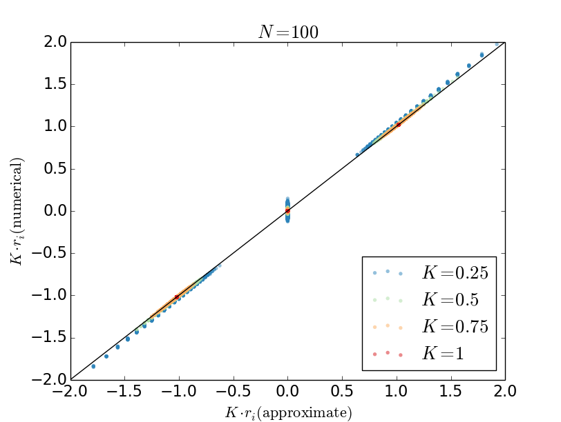
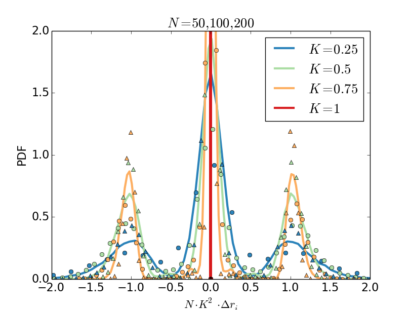
Figure 5: We generate random Erdos-Renyi topologies of mean connectivity $K$ and size $N$, where each link $w_{i\rightarrow j}=w=1$ (i.e. no asymmetry). The external flux is set to $J=10^{-2}$. We integrate numerically the associated master equation until stationarity, and calculate $r_{i}=(Np_{i}^{*}-1)/J$. (Left panel) We compare the numerical value of $r_{i}$ with the one given by the approximation of eq. (32), for all the nodes in the network and for $10^{3}$ randomly generated networks. Network size has been set to $N=100$. (Right panel) PDF of the error made in eq. (32), rescaled with the system size, for $N=50$ (circles), $N=100$ (solid line) and $N=200$ (triangles), for different connectivities with the same colorcode as on the left panel. In this case, we were able to capture also the scaling with the connectivity $K$. When rescaled properly, the location of the peaks approximately collapse, illustrating that the error made is $\Delta r_{i}=\mathcal{O}(K^{-2}N^{-1})$.

B.4 Distribution of $\dot{S}_{\mathrm{int}}$

We can obtain the PDF of $\dot{S}_{\mathrm{int}}$ assuming that, approximately, $\dot{S}_{1}$, $\dot{S}_{2}$ and $\dot{S}_{3}$ are independent random variables, so from Eqs. (24), (29) and (34) we find:

$$P\left(\dot{S}_{\mathrm{int}}=\dot{S}_{1}+\dot{S}_{2}+\dot{S}_{3}\right)\simeq\mathcal{N}\left((K(N-1)-2)w\sigma^{2},\sqrt{\left(4K\left(1-\frac{1}{N}\right)+\frac{8}{N}\right)\left(w\sigma^{2}\right)^{2}+\frac{4}{KN}\left(\sigma J\right)^{2}}\right)$$ (35)

$$\xrightarrow{\quad N\gg 1\quad}\mathcal{N}\left((KN-(2+K))w\sigma^{2},2\sqrt{K}w\sigma^{2}\right),$$ (36)

where in the last expression we have considered the leading contribution for large system size $N$.

Appendix C Distribution of $w_{\mathrm{eq}}$

The equivalent transition rate is defined close to equilibrium as $w_{\mathrm{eq}}=\frac{J}{p_{1}^{*}-p_{N}^{*}}$ when $\sigma=0$. Introducing the explicit form of $p_{i}^{*}\simeq(1+Jr_{i})/N$, where $r_{i}$ has the form of eq. (32) in large networks, we obtain:

$$w_{\mathrm{eq}}\simeq w\frac{k_{1}k_{N}}{k_{1}+k_{N}}.$$ (37)

Consequently, variability in $w_{\mathrm{eq}}$ comes, essentially, from the variability in the degrees of $k_{1}$ and $k_{N}$. We check numerically the validity of eq. (37). To this end, we generate master-equation systems described by random networks of size $N$ and connectivity $K$, and for each one we compare the corresponding value of $w_{eq}$ (obtained integrating numerically the master equation) with the one given by eq. (37). The result is plotted in Fig. 6 in log-log scale, showing a good agreement, especially for large network sizes and higher connectivities.

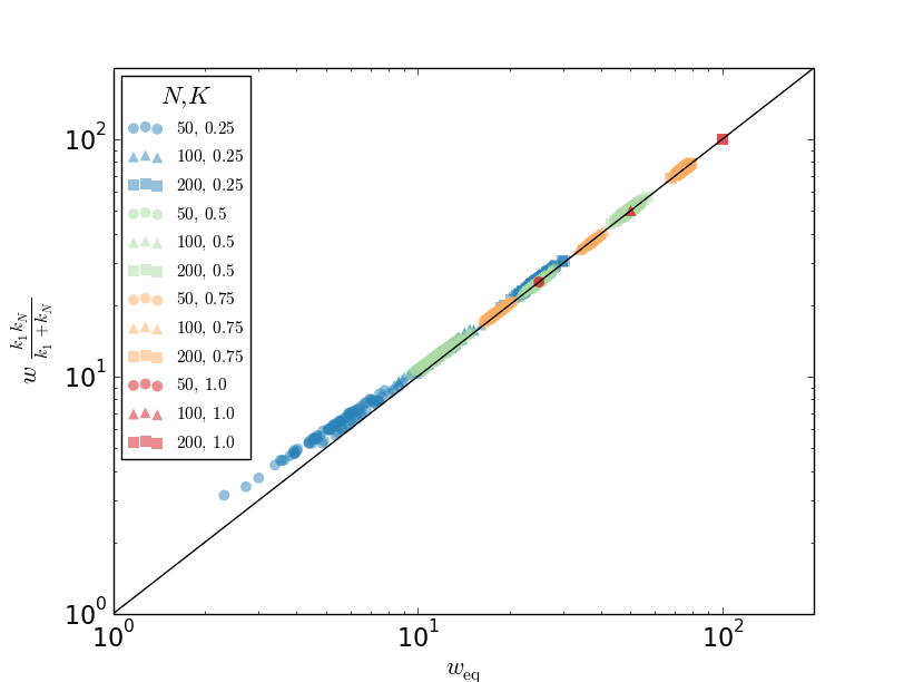
Figure 6: Comparison between $w_{\mathrm{eq}}$ with the approximation given by eq. (37) in symmetric master-equation systems with networks of size $N=50,100,200$ and connectivity $K=0.25,0.5,0.75,1$. All existing links in the network has a rate value $w=1$. For each network, $w_{\mathrm{eq}}$ has been obtained by integrating numerically the master equation with an additional external flux $J=0.01$, and then calculating $w_{\mathrm{eq}}=(p_{1}^{*}-p_{N}^{*})/J$.

The distribution of $w_{\mathrm{eq}}$ must be computed from the degree distribution of an Erdos-Renyi network of connectivity $K$, which is given by the binomial distribution $p(k)={N\choose k}K^{k}(1-K)^{N-k}$. For large $N$, the binomial distribution behaves as a Gaussian distribution with mean $NK$ and variance $NK(1-K)$, and neglecting the correlation between $k_{1}$ and $k_{N}$ we can write:

$$P(w_{\mathrm{eq}})\simeq\int_{-\infty}^{\infty}\int_{-\infty}^{\infty}\delta\left(w_{\mathrm{eq}}-w\frac{k_{1}k_{N}}{k_{1}+k_{N}}\right)P(k_{1})P(k_{N})dk_{1}dk_{N},$$ (38)

where the limits of the integral have been extended the whole real axis and $P(k)$ represents a Gaussian distribution $\mathcal{N}(NK,\sqrt{NK(1-K)})$. The non-linear dependency of $w_{eq}$ on $k_{1}$ and $k_{N}$ hinders the calculation of $P(w_{eq})$. However, as the Gaussian distributions becomes narrower (in relation to their mean) when $N$ increases, we can calculate the PDF in the limit of large $N$ using a saddle-point approximation. First, we write the delta function in terms of its Fourier representation:

$$P(w_{\mathrm{eq}})=\int_{-\infty}^{\infty}\int_{-\infty}^{\infty}\int_{-\infty}^{\infty}\frac{1}{2\pi}\exp\left[-i\alpha\left(w_{\mathrm{eq}}-w\frac{k_{1}k_{N}}{k_{1}+k_{N}}\right)\right]P(k_{1})P(k_{N})dk_{1}dk_{N}d\alpha.$$ (39)

Inserting the explicit form of $P(k)$, using the change of variables: $x_{1}=\dfrac{k_{1}}{KN}-1$, $x_{N}=\dfrac{k_{N}}{KN}-1$, and introducing the intensive variable $\hat{w}_{\mathrm{eq}}=\dfrac{w_{\mathrm{eq}}}{N}$, we obtain:

$$P(w_{\mathrm{eq}}) = \frac{NK}{(2\pi)^{2}(1-K)}\int_{-\infty}^{\infty}\int_{-\infty}^{\infty}\int_{-\infty}^{\infty}\exp\left[N\left(-i\alpha\left(\hat{w}_{\mathrm{eq}}-wK\frac{(1+x_{1})(1+x_{N})}{2+x_{1}+x_{N}}\right)-\frac{K}{2(1-K)}(x_{1}^{2}+x_{N}^{2})\right)\right]dx_{1}dx_{N}d\alpha$$ (40)

$$\equiv \frac{NK}{(2\pi)^{2}(1-K)}\int_{-\infty}^{\infty}\int_{-\infty}^{\infty}\int_{-\infty}^{\infty}\exp\left[NF(x_{1},x_{N},\alpha)\right]dx_{1}dx_{N}d\alpha.$$

The saddle-node approximation states that the integral $\int d^{d}z\exp[NF(\vec{z})]\simeq(2\pi/N)^{d/2}(-\det H(F)|_{\vec{z}^{*}})^{-1/2}\exp[Nf(\vec{z}^{*})]$ in the limit of large $N$, where $\vec{z}^{*}$ is the stationary point of $F$, $d$ its dimension and $H$ the Hessian matrix of $F$. Imposing $\partial_{x_{1}}F=\partial_{x_{N}}F=\partial_{\alpha}F=0$, we can find that in our case the stationary point is located at $x_{1}^{*}=x_{N}^{*}=2\frac{\hat{w}_{\mathrm{eq}}}{KN}-1$, $\alpha^{*}=4i\frac{kw-2\hat{w}_{\mathrm{eq}}}{k(1-k)w^{2}}$. After some calculations, and written in terms of the original variable $w_{\mathrm{eq}}$, we find:

$$P(w_{\mathrm{eq}})\simeq\frac{1}{\sqrt{2\pi\frac{NK(1-K)}{8}w^{2}\left(3-2\frac{wKN}{2w_{\mathrm{eq}}}\right)}}\exp\left[-\frac{\left(w_{\mathrm{eq}}-\frac{wKN}{2}\right)^{2}}{2\frac{NK(1-K)}{8}w^{2}}\right].$$ (41)

As the PDF concentrates around $w_{\mathrm{eq}}\simeq\frac{wKN}{2}$ when $N$ increases, $\left(3-2\frac{wKN}{2w_{\mathrm{eq}}}\right)\simeq 1$. Therefore, we finally obtain that

$$P\left(\frac{w_{\mathrm{eq}}}{w}\right)\simeq\mathcal{N}\left(\frac{NK}{2},\sqrt{\frac{1}{8}NK(1-K)}\right).$$ (42)

We can collapse data of $w_{\mathrm{eq}}$ for different ensembles into a single PDF by substracting the mean and rescaling by the standard deviation as obtainable from eq. (42). Results are shown in Fig. 7. Deviations from a perfect collapse (that are higher for smaller networks) must stem from finite size corrections to the scaling formulas (see Section C.1).

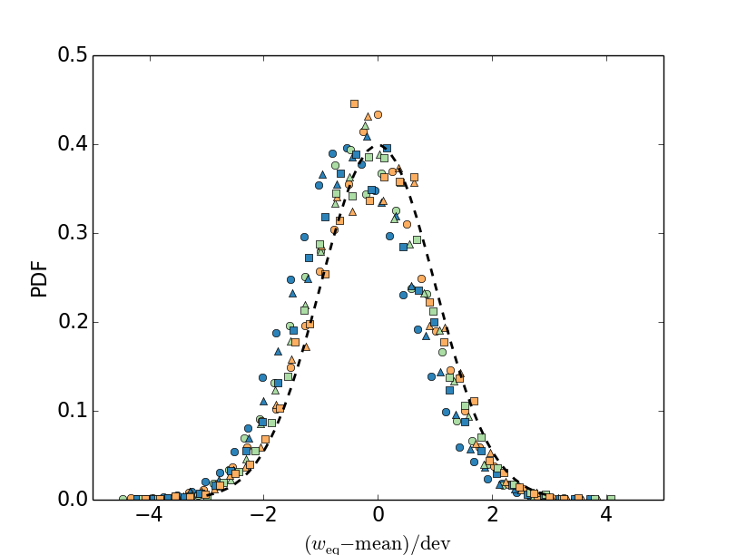
Figure 7: Collapse of the PDF for 9 datasets of $w_{\mathrm{eq}}$, for $K=0.25$ (blue), $K=0.5$ (green) and $K=0.75$ (yellow), and for each one, for $N=50$ (circles), $N=100$ (triangles) and $N=200$ (squares) (same datasets of Fig. 6), obtained by subtracting the corresponding mean $NKw/2$ and dividing by the standard deviation $NK(1-K)w/8$ on each data (Eqs. (44) and (45) for the left panel and Eqs. (46) and (47) for the right one). Dashed lines represent a Gaussian distribution of zero mean and unit variance. Deviations stem from finite size corrections, and indeed PDFs for larger system sizes fit better the Gaussian distribution.

C.1 Calculation of $\langle f(w_{\mathrm{eq}})\rangle$

We can calculate the expected value of some general function $f(w_{\mathrm{eq}})$ using the asymptotic form of $P(w_{\mathrm{eq}})$, Eq. (42). However, it can be useful to calculate next-to-leading order terms as it follows. We first write the expected value as

$$\langle f(w_{\mathrm{eq}})\rangle=\int_{-\infty}^{\infty}\int_{-\infty}^{\infty}f\left(w\frac{k_{1}k_{N}}{k_{1}+k_{N}}\right)P(k_{1})P(k_{N})dk_{1}dk_{N}=\sum_{n,m=0}^{\infty}\frac{\mu_{2n}\mu_{2m}}{(2n)!(2m)!}\left.\frac{\partial f}{\partial k_{1}^{2n}\partial k_{N}^{2m}}\right|_{k_{1}=k_{N}=KN},$$ (43)

where $\mu_{i}$ is the $i$-th central moment of a Gaussian distribution of mean $KN$ and variance $NK(1-K)$, and them simply truncate the series at the desired order. Using this expression, it is straightforward to calculate $\langle w_{\mathrm{eq}}\rangle$ expanding $\frac{k_{1}k_{N}}{k_{1}+k_{N}}$ up to the the forth moment:

$$\langle w_{\mathrm{eq}}\rangle=w\left(\frac{KN}{2}-\frac{1-K}{4}\right)-\frac{(1-K)^{2}}{8KN}+\mathcal{O}(N^{-2})$$ (44)

and its variance $\langle\langle w_{\mathrm{eq}}^{2}\rangle\rangle=\langle w_{\mathrm{eq}}^{2}\rangle-\langle w_{\mathrm{eq}}\rangle^{2}$ from the expansion of $\left(\frac{k_{1}k_{N}}{k_{1}+k_{N}}\right)^{2}$:

$$\langle\langle w_{\mathrm{eq}}^{2}\rangle\rangle=\frac{w^{2}}{8}\left(NK(1-K)+2(1-K)^{2}\right)+\mathcal{O}(N^{-1}).$$ (45)

As expected, the leading orders agree with the mean and variance of $P(w_{\mathrm{eq}})$, eq. (42). Similarly, it is also useful to compute the mean and variance of $w_{\mathrm{eq}}^{-1}$ using the similar procedure; the result is:

$$\langle w_{\mathrm{eq}}^{-1}\rangle = \frac{2}{wKN}\left(1+\frac{1-K}{KN}\right)+\mathcal{O}(N^{-3})$$ (46)

$$\langle\langle(w_{\mathrm{eq}}^{-1})^{2}\rangle\rangle = \frac{2(1-K)}{w^{2}(KN)^{3}}\left(1+20\frac{1-K}{KN}\right)+\mathcal{O}(N^{-5}).$$ (47)

Let us notice that the leading term of $\langle w_{\mathrm{eq}}^{-1}\rangle$ is the one used in the bottom panel of Fig. 3.

Appendix D Distribution of $\epsilon_{\mathrm{eq}}$

To compute the unbalance parameter $\epsilon_{\mathrm{eq}}$, we set the external current to $J=0$. In this setting, and for small asymmetry values, $\sigma\ll 1$, the stationary probability can be written as $p_{i}^{*}=1/N(1+\sigma q_{i})$, so $\epsilon_{\mathrm{eq}}$ can be computed as:

$$\epsilon_{\mathrm{eq}}=\frac{p_{1}^{*}-p_{N}^{*}}{\sigma}=\frac{q_{1}-q_{N}}{N}.$$ (48)

Introducing the approximation given by eq. (27) into the equation above, one finds the explicit formula:

$$\epsilon_{\mathrm{eq}}=\frac{1}{N}\left(\frac{1}{k_{N}}\sum_{j}A_{Nj}D_{Nj}-\frac{1}{k_{1}}\sum_{j}A_{1j}D_{1j}\right).$$ (49)

At this step, we neglect the heterogeneity in the connectivity degree and set $k_{1}\simeq k_{N}\simeq KN$. Reminding that $D_{ij}=-D_{ji}$ are independent Gaussian variables for each pair of links with zero mean and variance 2, for large networks the Central Limit Theorem gives:

$$P(\epsilon_{\mathrm{eq}})\simeq\mathcal{N}\left(0,\frac{2}{N\sqrt{KN}}\right),$$ (50)

where we have neglected a small correction arising if nodes $1$ and $N$ are connected (i.e. when $A_{1N}=1$); in such a case the first and second term in eq. (49) would not be completely uncorrelated, as $D_{1N}=-D_{N1}$. In any case, this correction is negligible for large N.

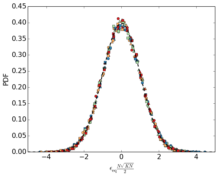
Figure 8: Collapse of different $P(\epsilon_{\mathrm{eq}})$ for asymmetric master-equation systems in ensembles of $10^{4}$ networks of size $N=50$ (circles), $N=100$ (triangles) and $N=200$ (squares), and for each one, for connectivities $K=0.25$ (blue), $K=0.5$ (green) and $K=0.75$ (yellow). Link weights in the network are independent Gaussian variables of mean $w=1$ and standard deviation $w\sigma=0.01$. For each network, $\epsilon_{\mathrm{eq}}$ has been obtained by integrating numerically the master equation with the external flux $J=0$, and then calculating $\epsilon_{\mathrm{eq}}=(p_{1}^{*}-p_{N}^{*})/\sigma$. Dark dashed line represents the Gaussian distribution of zero mean and unit variance. The collapse has been obtained by dividing each value of $\epsilon_{\mathrm{eq}}$ by its corresponding standard deviation obtained analytically, $2/(N\sqrt{KN})$.

Appendix E Deviations from Joule’s law

Close to equilibrium, we can write the total entropy production for asymmetric systems at stationarity as $\dot{S}^{*}=\dot{S}_{\mathcal{J}}+N\epsilon_{\mathrm{eq}}\sigma J+\dot{S}_{\mathrm{int}}$ (see main text). Therefore, deviations from Joule’s law, $\delta\dot{S}_{\mathcal{J}}=\dot{S}^{*}-\dot{S}_{\mathcal{J}}$ can be obtained combining the Gaussian distributions of $\epsilon_{\mathrm{eq}}$ (eq. (50)) and $\dot{S}_{\mathrm{int}}$ (eq. (36)):

$$P\left(\delta\dot{S}_{\mathcal{J}}=\dot{S}_{\mathrm{int}}+N\epsilon_{\mathrm{eq}}\sigma J\right)\simeq\mathcal{N}\left((NK-(2+K))w\sigma^{2},\sqrt{4K\left(w\sigma^{2}\right)^{2}+\frac{4}{KN}\left(\sigma J\right)^{2}}\right)\xrightarrow{\quad NK\gg 1\quad}\mathcal{N}\left(NKw\sigma^{2},2\sqrt{K}w\sigma^{2}\right).$$ (51)

We can see that, for large systems, the contribution given by $\epsilon_{\mathrm{eq}}$ is negligible, obtaining the same result as in eq. (36).

References

Jiang et al. (2004)D.-Q. Jiang, M. Qian, and M.-P. Qian, Mathematical theory of nonequilibrium steady
states: on the frontier of probability and dynamical systems (Springer, 2004).
Andrieux and Gaspard (2007)D. Andrieux and P. Gaspard, J. Stat. Phys. 127, 107 (2007).
Jaynes (1957a)E. T. Jaynes, Phys. Rev. 106, 620 (1957a).
Jaynes (1957b)E. T. Jaynes, Phys. Rev. 108, 171 (1957b).
Martyushev and Seleznev (2006)L. Martyushev and V. Seleznev, Phys. Rep. 426, 1
(2006).
Dewar (2003)R. Dewar, J. Phys. A: Math. Gen. 36, 631 (2003).
Prigogine (1955)I. Prigogine, Thermodynamics of
irreversible processes (Thomas, 1955).
Goldstein and Lebowitz (2004)S. Goldstein and J. L. Lebowitz, Physica D 193, 53 (2004).
Lebowitz and Spohn (1999)J. L. Lebowitz and H. Spohn, J.
Stat. Phys. 95, 333 (1999).
Tomé and de Oliveira (2012)T. Tomé and M. J. de Oliveira, Phys. Rev. Lett. 108, 020601 (2012).
Ziener et al. (2015)R. Ziener, A. Maritan, and H. Hinrichsen, J.
Stat. Mech. Theor. Exp. 2015, P08014 (2015).
Jiu-Li et al. (1984)L. Jiu-Li, C. Van
Den Broeck, and G. Nicolis, Z. Phys. B 56, 165 (1984).
Maes and Netočnỳ (2003)C. Maes and K. Netočnỳ, J. Stat. Phys. 110, 269 (2003).
Zia and Schmittmann (2007)R. Zia and B. Schmittmann, J. Stat. Mech. Theor. Exp. 2007, P07012 (2007).
Harris and Schütz (2007)R. J. Harris and G. M. Schütz, J. Stat. Mech. Theor. Exp. 2007, P07020 (2007).
Zia and Schmittmann (2006)R. K. Zia and B. Schmittmann, J. Phys. A: Math. Gen. 39, L407 (2006).
Szabó et al. (2010)G. Szabó, T. Tomé,
and I. Borsos, Phys. Rev.
E 82, 011105 (2010).
Wigner (1955)E. P. Wigner, Ann. Math. , 548 (1955).
Crisanti et al. (2012)A. Crisanti, G. Paladin, and A. Vulpiani, Products of Random Matrices: in
Statistical Physics, Vol. 104 (Springer Science & Business Media, 2012).
Allesina and Tang (2012)S. Allesina and S. Tang, Nature 483, 205 (2012).
Sompolinsky et al. (1988)H. Sompolinsky, A. Crisanti, and H.-J. Sommers, Phys. Rev. Lett. 61, 259 (1988).
Baiesi et al. (2009)M. Baiesi, C. Maes, and B. Wynants, Phys. Rev. Lett. 103, 010602 (2009).
Newman (2003)M. E. Newman, SIAM
Rev. 45, 167 (2003).
Kleidon et al. (2010)A. Kleidon, Y. Malhi, and P. Cox, Philos. Trans. R. Soc. Lond., B, Biol. Sci. 365, 1297 (2010).
Barabási and Albert (1999)A.-L. Barabási and R. Albert, Science 286, 509 (1999).