NoSOCS in SDSS. VI. The Environmental Dependence of AGN in Clusters and Field in the Local Universe

Abstract

We investigated the variation in the fraction of optical active galactic nuclei (AGN) hosts with stellar mass, as well as their local and global environments. Our sample is composed of cluster members and field galaxies at $z\leq 0.1$ and we consider only strong AGN. We find a strong variation in the AGN fraction (F_AGN) with stellar mass. The field population comprises a higher AGN fraction compared to the global cluster population, especially for objects with log $M_{*}>10.6$. Hence, we restricted our analysis to more massive objects. We detected a smooth variation in the F_AGN with local stellar mass density for cluster objects, reaching a plateau in the field environment. As a function of clustercentric distance we verify that F_AGN is roughly constant for R $>$ R₂₀₀, but show a steep decline inwards. We have also verified the dependence of the AGN population on cluster velocity dispersion, finding a constant behavior for low mass systems ($\sigma_{P}\lesssim 650-700$ km s^-1). However, there is a strong decline in F_AGN for higher mass clusters ($>$ 700 km s^-1). When comparing the F_AGN in clusters with or without substructure we only find different results for objects at large radii (R $>$ R₂₀₀), in the sense that clusters with substructure present some excess in the AGN fraction. Finally, we have found that the phase-space distribution of AGN cluster members is significantly different than other populations. Due to the environmental dependence of F_AGN and their phase-space distribution we interpret AGN to be the result of galaxy interactions, favored in environments where the relative velocities are low, typical of the field, low mass groups or cluster outskirts.

1 Introduction

A key issue in the understanding of galaxy formation and evolution is related to the triggering mechanisms of active galactic nuclei. Although supermassive black holes (SMBHs) are common in the central parts of virtually all massive galaxies, it is not clear why just a few objects display strong nuclear activity due to matter accretion. Different mechanisms are possible to feed the inflow of gas to the galaxy centers activating their nuclei. Among those are major and minor mergers, bar influence, disc instability and tidal effects (Moore et al., 1996; Elmegreen et al., 1998; Springel et al., 2005; Genzel et al., 2008). Some of those (such as mergers and interactions) are also known for accelerating the star formation rate (SFR), pointing to a co-evolution between black hole growth and star formation activity in galaxies (Silverman et al., 2008; Hickox et al., 2014; Azadi et al., 2015; Wang et al., 2015; Alberts et al., 2016).

As galaxy interactions and mergers are environment related processes the investigation of the nuclear activity dependence on environment may be paramount on providing clues on the AGN triggering. Hence, the investigation of the AGN properties and frequency in the field, groups and clusters can be important for understanding those system’s evolution. Several studies tackle this issue, finding in general an anti-correlation between AGN fraction and environmental density, so that fewer AGN are found in clusters compared to the field (Dressler et al., 1999; Kauffmann et al., 2004; Alonso et al., 2007). Discrepancies among different studies are generally explained by the use of different samples (in terms of luminosity and mass, and wavelength selection), and environment definitions. Regarding the use of AGN selected in different wavelengths the environmental dependence and triggering mechanism for AGN selected in the radio may be different from optical and mid-IR selected AGN (Satyapal et al., 2014; Ellison et al., 2015), as well as X-rays (Martini et al., 2013; Goulding et al., 2014).

Besides the local environment, the global may also be relevant to the AGN population. For instance, Popesso & Biviano (2006) find an anti-correlation between AGN fraction and cluster velocity dispersion, so that F_AGN decreases as $\sigma_{P}$ increases. The authors interpret this result as a consequence of the galaxy-galaxy merger inefficiency in clusters, as cluster galaxies have high relative velocities. Hence, the AGN phenomenon is more common in the field and low mass groups. The global environment can also be indicated by how long a galaxy inhabit a cluster, as recent arrivals have been less affected by the cluster potential. We can estimate how long since a galaxy infall from their location in the cluster phase-space (Oman et al., 2013). Hence, we can investigate the AGN distribution in phase-space trying to understand their evolution within clusters.

Finally, another important factor on assessing the environment influence (actually the cluster environment) is the dynamical stage of such systems. Pimbblet et al. (2013) investigate the AGN fraction in six nearby relaxed clusters. They use only systems with no substructure signs as they argue mergers of groups and clusters may locally boost AGN activity, biasing the analysis. Popesso & Biviano (2006) also avoid clusters with substructure, but for a different reason. As they investigate the F_AGN-$\sigma_{P}$ connection they did not want to have systems with possible wrong values for $\sigma_{P}$.

Nonetheless, despite what is said above, it is essential to emphasize the variation of F_AGN with environment is not a consensus in the literature, as there are many studies pointing to no environment connection in the number of AGN found. For instance, Miller et al. (2003) find that the fraction of galaxies hosting AGN does not change from the central parts of clusters all the way to the field. von der Linden et al. (2010) results also point to an independence of F_AGN and clustercentric radius, but only for powerful AGN hosted by star-forming galaxies. The same is not true for weak optical AGN hosted by red galaxies. The lack of environment influence is also supported by the work of Sabater et al. (2015), who find the local density and one-to-one interactions to have little impact on the AGN activity. del Pino et al. (2017) also point to no environmental dependence on F_AGN for objects in the region of the Abell 901/2 multi-cluster system.

This work is the sixth of a series aiming to investigate cluster and galaxies’ properties at low redshifts ($z\leq 0.1$). On this current paper we focus on the investigation of the variation of the AGN population as function of environment and stellar mass. Our data set is composed of objects in two complementary luminosity ranges ($M_{r}\leq M^{*}+1$ and $M^{*}+1<M_{r}\leq M^{*}+3$), where $M^{*}$ is the characteristic magnitude of the luminosity function in the $r-$band. However, in the current work, as explained in $\S$ 3, we apply a stellar mass cut (log $M_{*}>10.6$) so that nearly all objects are in the bright regime.

We organized this paper in the following way: $\S$2 has the data description, where we define the cluster and field samples, and discuss the local galaxy density estimates, the stellar population properties, and the AGN sample. In $\S$3 we present the relation between AGN fraction and stellar mass. The environmental variation of the AGN population is investigated in $\S$4. We search for the connection to the local and global environment, indicated by cluster velocity dispersion and dynamical stage. The possible dependence of the environmental variation on galaxy host type is searched in $\S$5. In $\S$6 we compared the AGN distribution in phase-space to other three populations. Our main results are summarize in $\S$7. The cosmology assumed in this work considers $\Omega_{\rm m}=$0.3, $\Omega_{\lambda}=$0.7, and H${}_{0}=100$ $\rm h$ $\rm km$ $s^{-1}$ Mpc^-1, with $\rm h$ set to 0.7. For simplicity, in the following we are going to use the term “cluster” to refer loosely to groups and clusters of galaxies.

2 Data

This work is based on a sample of 6415 galaxies belonging to 152 groups and clusters and 4676 selected as field galaxies. Our clusters span the range $150\la\sigma_{P}\la 950$ km s^-1, or the equivalently in terms of mass, $10^{13}\la M_{200}\la 10^{15}M_{\odot}$. The cluster and field samples are restricted to $z\leq 0.100$. In the next two subsections we briefly describe the cluster and field samples. We also describe the main galaxy properties used in this paper, as well as the AGN selection and the local density estimates. Further details on the construction of those two samples can be found in the previous papers of this series (papers I to V).

2.1 Cluster Sample

The cluster sample was originally selected from the digitized version of the Second Palomar Observatory Sky Survey (POSS-II; DPOSS, Djorgovski et al. 2003; Gal et al. 2004; Odewahn et al. 2004), and it is named the Northern Sky Optical Cluster Survey (NoSOCS, Gal et al. 2003; Lopes et al. 2004; Gal et al. 2009). In paper I we defined this low-$z$ cluster sample from the supplemental version of the NoSOCS (Lopes et al., 2004), re-estimating photometric redshifts as in Lopes (2007). This low-redshift sample was complemented with more massive systems from the Cluster Infall Regions in SDSS (CIRS) sample (Rines & Diaferio 2006, hereafter RD06). Most of the galaxy and cluster properties, including the local density estimates (for field and cluster galaxies) were derived using the 7th Sloan Digital Sky Survey (SDSS) release (DR7). The exception is given by the stellar population properties (see below) that were derived from the SDSS DR8.

The redshift limit of the sample ($z=0.100$) is due to incompleteness in the SDSS spectroscopic survey for higher redshifts, where galaxies fainter than $M^{*}+1$ are missed, biasing the dynamical analysis (see discussion in section 4.3 of Lopes et al. 2009a). We eliminated interlopers and selected cluster members using the “shifting gapper” technique (Fadda et al., 1996; Lopes et al., 2009a), applied to all galaxies with spectra available within a maximum aperture of 2.50 h^-1 Mpc, and within $\pm$ 4000 km s^-1 of the cluster redshift. After selecting cluster members we perform a virial analysis, obtaining estimates of velocity dispersion, physical radius and mass ($\sigma_{P}$, $R_{500}$, $R_{200}$, $M_{500}$ and $M_{200}$; details in paper I).

For the clusters with at least five galaxy members within R₂₀₀ we also have a substructure estimate, based on the DS (or $\Delta$) test (Dressler & Shectman, 1988). Another substructure estimate was derived from the Hellinger Distance (HD) measure, but in that case we impose a minimum of 20 galaxies within R₂₀₀ (see Ribeiro et al. 2013b; de Carvalho et al. 2017). We also estimated X-ray luminosity ($L_{X}$, using ROSAT All Sky Survey data), optical luminosity ($L_{opt}$) and richness (N_gals, Lopes et al. 2009a, b). The centroid of each NoSOCS cluster is a luminosity weighted estimate, which correlates well with the X-ray peak (see Lopes et al. 2006).

2.2 Field Sample

The galaxy field sample is constructed in an independent manner of the cluster sample above, meaning it is not taken as the interlopers found within the maximum sampling cluster regions (2.50 h^-1 Mpc, and within $\pm$ 4000 km s^-1). As described in Lopes, Ribeiro & Rembold (2014); Lopes et al. (2016) we select as field objects those galaxies from the whole SDSS DR7 that are not associated to a group or cluster. Our cluster catalog used as reference is the one from Gal et al. (2009), containing more than 15,000 cluster candidates over 11,411 deg². Our approach is very conservative, so that a galaxy is said to belong to the field if it is not found within 4.0 Mpc and not having a redshift offset smaller than 0.06 of any cluster from Gal et al. (2009). Note the clusters in that catalog have a photometric (not spectroscopic) redshift estimate. We select more than 60,000 field galaxies, but work with a smaller subset (randomly chosen). The field sample we used has 2,936 galaxies at $z\leq$ 0.100 with $M_{r}\leq M^{*}+1$, and 1,740 at $z\leq$ 0.045 with $M^{*}+1<M_{r}\leq M^{*}+3$. The local density is estimated for those objects (see below) in the same way as done for the cluster members.

It is important to stress this field sample is based on a comparison to one cluster catalog (Gal et al., 2009). Cluster samples are generally complete for rich systems, but not for the smaller mass groups and clusters. Due to that some field objects may actually belong to small groups, that are not listed by Gal et al. (2009) (and could also be missing from other cluster catalogs). The number of “field objects” that could be group members is expected to be small, and most importantly, their local densities are much smaller than typical values of the central regions of groups and clusters, being at most comparable to the values found in the outskirts of those systems.

2.3 Absolute Magnitudes and Colours

In the current work we consider the stacked properties of galaxies in our sample. That is done using the radial offset in units of $R_{200}$ (only for member galaxies), absolute magnitudes, colours and local densities of all galaxies in our cluster and field samples. The absolute magnitudes of each galaxy in five SDSS bands ($ugriz$) are derived using the formula: $M_{x}=m_{x}-DM-kcorr-Qz$ ($x$ is one of the five SDSS bands we used), DM is the distance modulus (using the galaxy redshift), $kcorr$ is the k$-$correction and $Qz$ ($Q=-1.4$, Yee & López-Cruz 1999) is a mild evolutionary correction applied to the magnitudes. Rest-frame colours are also derived for all objects. The magnitudes we obtained from the SDSS are de-reddened model magnitudes (see paper I). We consider the k$-$corrections available in the SDSS database, for each galaxy and band.

2.4 The stellar population properties

A variety of galaxy properties were obtained by different research groups for the SDSS. These parameters consider galaxy spectra or the broad band galaxy photometry, and are derived from spectral energy distribution (SED) fitting of stellar population synthesis models. In the current work we consider parameters derived from the “galSpec” analysis provided by the MPA-JHU group (from the Max Planck Institute for Astrophysics and the Johns Hopkins University; Brinchmann et al. 2004). A brief description of those parameters is given below.

2.4.1 MPA-JHU

The galaxy properties from MPA-JHU, named “galSpec”, were obtained for DR8 galaxy spectra (nearly all of which were in DR7). The galaxy parameters we used in the current work are the BPT classification (Baldwin, Phillips & Terlevich, 1981), the stellar mass and the star formation rate. From the BPT diagram the MPA-JHU group classified galaxies into the following categories: “Star Forming”, “Composite”, “AGN”, “Low S/N Star Forming”, “Low S/N AGN”, and “Unclassifiable”. This classification using the BPT diagram considers four emission lines (see Fig. 1 of Brinchmann et al. 2004) and requires S/N $>3$ for all lines. In particular a “Low S/N AGN” has [N_II]6584/H${\alpha}$ $>0.6$ (and S/N $>3$ in both lines), but has [O_III]5007 and/or H${\beta}$ with low S/N. “Low S/N Star Forming” galaxies are those with S/N $>2$ in H${\alpha}$ after most galaxies with an AGN contribution to their spectra are removed.

Besides the galaxy classification described above, we also consider the total stellar mass and star formation rate values (SFRs) from “galSpec”. The stellar masses are based on model magnitudes. The SFRs are computed within the galaxy fiber aperture and are based on the nebular emission lines as described in Brinchmann et al. (2004). The galaxy photometry is used outside of the fiber (Salim et al., 2007). For AGN and galaxies with weak emission lines the SFRs estimates are derived from the photometry. Due to the minimum criteria required by the MPA-JHU group (e.g., redshift, S/N) not all galaxies in our sample are matched to the MPA-JHU data set. Hence, our sample with MPA-JHU values have 4,953 bright and 1,297 faint member galaxies, and also 2,864 bright and 1,672 faint field galaxies. That is 97$\%$ of the original sample.

2.5 The AGN population

As mentioned above the object classification we consider is based on a BPT diagram. In the current study we investigate the dependence of the AGN population on stellar mass, local and global environment. The latter is traced by the parent cluster mass and can be also studied by comparing field and cluster objects. We note the AGN class from “galSpec” already excludes LINERs, objects that are not primary powered by nuclear activity (Schawinski et al., 2010; Singh et al., 2013). Objects named “Low S/N Star Forming” represent a different class (as described above) and are not part of our sample. To further reduce contamination from objects not mainly dominated by nuclear activity we do not include “Composite” objects in our AGN sample. Hence, our list of AGN considers only objects classified as “AGN” (excluding LINERs) from “galSpec” (see §2.4.1 above). Note that some authors also include “Composite” objects (Sohn et al., 2013; Bitsakis et al., 2015) leading to higher AGN fractions than what we show below.

2.6 Local Galaxy Density Estimates

For the current work we adopt the $\Sigma_{5}$ local galaxy density estimator. That is motivated by the conclusions of Muldrew et al. (2012) who find that nearest neighbor methods are superior on tracing the local environment. The choice of the rank of the density-defining neighbor ($n$) is also important. We chose to work with $n=5$ since that is typically smaller than the number of galaxies we have per cluster and is a common estimate in the literature. The local galaxy density estimates are derived as follows. For each galaxy in our sample we compute the projected distance, d₅, to the 5th nearest galaxy around it. We also impose to the neighbor search a maximum velocity offset of 1000 $km$ $s^{-1}$, and a maximum luminosity, which we adopt as $M^{*}+1.0$. The local density $\Sigma_{5}$ is simply given by 5/$\pi$d${}_{5}^{2}$, and is measured in units of galaxies/Mpc². Finally, we also take in account the fiber collision issue when deriving galaxy densities. The procedure is well described in La Barbera et al. (2010); Lopes, Ribeiro & Rembold (2014).

2.6.1 Stellar Mass Density Estimates

It is well know that the central parts of clusters - normally the most dense regions in the Universe - are inhabited by the most luminous and massive galaxies, so that a correlation between local galaxy number density and stellar mass is expected. Nonetheless, the scatter on this relation may not be negligible and the environmental dependence of galaxy properties may be better traced by the the galaxy stellar mass density, instead of simply the galaxy number density. Hence, we also computed the former. We adopt the same procedure as above, but added the stellar mass of the five nearest neighbors, instead of their numbers. The local stellar mass density $\Sigma_{5*}$ is then given by S${}_{5}^{*}$/$\pi$d${}_{5}^{2}$, where S${}_{5}^{*}$ is the sum of the stellar masses of the five nearest neighbours. $\Sigma_{5*}$ is measured in units of M_⊙/Mpc². In Fig. 1 we display a comparison of the galaxy stellar mass density ($\Sigma_{5*}$) vs the numerical density ($\Sigma_{5}$) for the cluster and field galaxies. We can see a good correlation between the two estimates, stretching from the low density field environment to the high densities of cluster cores. Hence, for the current work we adopted the local galaxy stellar mass density ($\Sigma_{5*}$) as the tracer of the local environment. The error bars in the figure indicate the 1$\sigma$ standard error on the “biweight location estimate”, which is a resistant and robust estimator. It is known to be superior to the mean and median estimates, both in terms of resistance and robustness. See Beers et al. (1990) for a proper definition of the biweight estimator, as well for a comparison of its performance to other estimators.

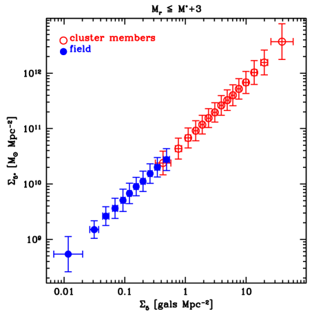
Figure 1: Comparison between the galaxy stellar mass density ($\Sigma_{5*}$) and the galaxy number density ($\Sigma_{5}$), for cluster (red open circles) and field (blue filled symbols) galaxies. The error bars indicate the 1$\sigma$ standard error on the biweight location estimate.

3 The AGN Fraction by Stellar Mass

We exhibit in Fig. 2 the variation of the AGN fraction (F_AGN) of our sample as a function of galaxy stellar mass, for cluster and field objects. F_AGN is defined here as the number of objects classified as AGN ($\S$2.5) divided by the total number of galaxies in our sample (no luminosity or morphological cuts are applied). As expected there is a clear increase in the number of AGN as we go from low to high-mass objects (Best et al., 2005; Brusa et al., 2009; Pimbblet et al., 2013). However, it is interesting to note that the AGN fraction is normally higher in the field than in clusters, especially for log $M_{*}\gtrsim 10.6$. Hence, from this figure we can also detect the impact of global environment, as at fixed stellar mass the fraction of AGN decreases as we move from the field to clusters. Due to possible incompleteness in the AGN selection for low luminosity (massive) objects, we decided to consider only massive objects (log $M_{*}>10.6$) in the current work. Taking this limit we also enforce a clearer separation between field and clusters. Another important reason to drop objects with log $M_{*}\leq 10.6$ is the fact that there is no strong environmental variation in the AGN fraction for those low mass objects (Pimbblet et al., 2013). We have also found that. Hence, we chose to exclude the low mass regime as its inclusion weakens the connection between AGN fraction and environment (see below).

After applying the stellar mass cut the sample decreases to 3,118 member galaxies and 1,561 field galaxies. That represents $\sim$ 50% of the cluster sample and $\sim$ 34% of the field sample described in the end of $\S$ 2.4.1. However, this stellar mass cut effectively is a luminosity cut, so that the vast majority of objects ($>$ 99%) surviving is in the bright regime ($M_{r}\leq M^{*}+1$; $\S$ 2.3). Considering the bright samples described in $\S$ 2.4.1 (4,953 members and 1,672 field objects), after applying the stellar mass cut we ended up with $\sim$ 63% of those bright cluster members and $\sim$ 54% of the bright field objects. Regarding the global AGN fractions, in the cluster and field environment, after we apply the stellar mass cut we have the following: out of the 3,118 massive cluster members we have 133 ($\sim$ 4,3%) which are AGN. In the field, out of the 1,561 massive objects we find 139 ($\sim$ 8,9%) AGN.

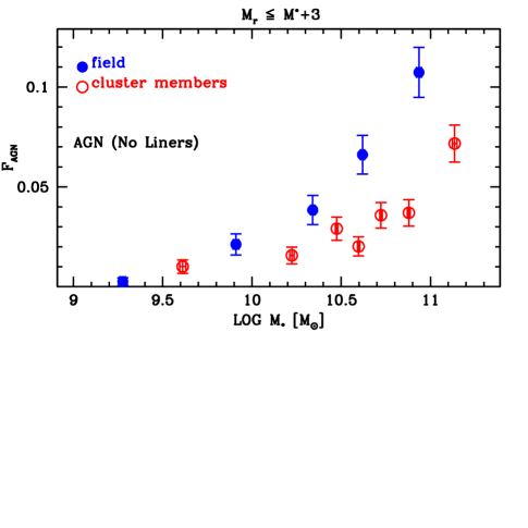
Figure 2: Variation of AGN fraction as a function of galaxy stellar mass, for cluster (red open circles) and field (blue filled circles) objects. The error bars indicate the 1$\sigma$ standard error on the biweight location estimate.

4 The Environmental Variation of the AGN Population

4.1 Local Environment Dependence

4.1.1 Variation with Galaxy Stellar Mass Density

In this section, we investigate the variation of the AGN fraction with local environment, given by the galaxy stellar mass density. In Fig. 3 we show the variation in the relative number of AGN as a function of local galaxy stellar mass density ($\Sigma_{5*}$). From the low to the high density regime in the field we detect a small increase in the fraction of AGN. However, from the outskirts of clusters (low densities) to their cores (high density environment) we can see a strong decrease in the AGN fraction as a function of local stellar mass density. A possible explanation for those results is that nuclear activity is triggered by mergers, which may be preferable in the higher density field environment or within low mass groups and the outskirts of clusters, which is the case for 10.0 $<$ log $\Sigma_{5*}<$ 10.6. In such low $\Sigma_{5*}$ regions the relative galaxy velocities are small, favouring galaxy mergers (see $\S$4.2.1 below).

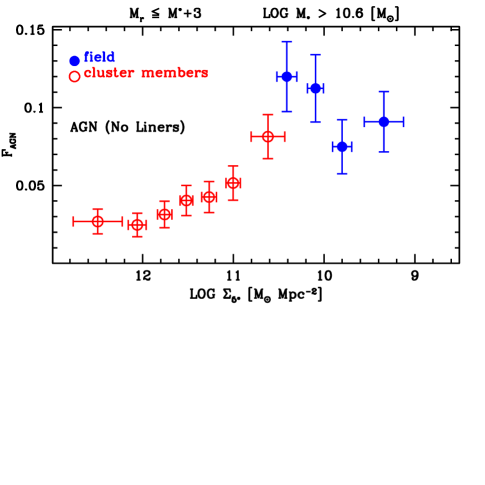
Figure 3: Dependence of AGN fraction as a function of local galaxy stellar mass density ($\Sigma_{5*}$), for cluster (red open circles) and field (blue filled circles) objects. The error bars indicate the 1$\sigma$ standard error on the biweight location estimate.

4.1.2 Variation with Clustercentric Distance

In Fig. 4 we display the relation between the AGN fraction and clustercentric distance for cluster members. The field value is also displayed as a reference. We can see a clear variation in F_AGN as a function of normalized radial offset. Inside R₂₀₀ there is a steep decline in the AGN fraction. However, outside R₂₀₀ the AGN fraction is nearly constant. Two more important results can still be seen on this figure. First we see the field value is significantly larger than the fractions within clusters, even in their outskirts. Second, there is a small decrease in the AGN fraction for R $>$ 1.5R₂₀₀, but that is not significant, and the fraction at R $>$ 2R₂₀₀ is at least two times larger than found in the cluster cores. Pimbblet et al. (2013) mention it is common to find in the literature results pointing to no difference between cluster and field AGN fractions (but see the results of Sohn et al. 2013 for different conclusions). Pimbblet et al. (2013) also claim no significant difference between the results in the core and at R $\sim$ 2R₂₀₀. One possible explanation for those discrepancies is the mix of galaxy host types. Sohn et al. (2013) find a significant difference between field and clusters, but mainly for AGN hosted by ETGs. That is corroborated by Fig. 9 ($\S$5). The other reason, possibly the most important, is the inclusion of low mass objects. We notice that low mas objects (log $M_{*}\leq$ 10.6) display similar AGN fractions in clusters and the field. The difference in the central and outskirts of clusters is also not significant. That can also be seen in Fig. 6 of Pimbblet et al. (2013).

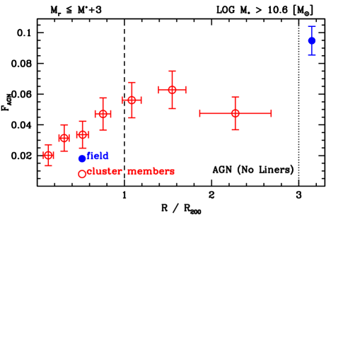
Figure 4: Variation of AGN fraction as a function of clustercentric distance for the cluster objects (red open circles). The corresponding estimate for the field is indicated by the blue filled circle. The error bars indicate the 1$\sigma$ standard error on the biweight location estimate.

4.2 Global Environment Dependence

4.2.1 Connection to Cluster Velocity Dispersion

We examine the dependence of F_AGN on the parent cluster mass, indicated by the velocity dispersion. That is shown in Fig. 5. There is a constant relation between AGN fraction and $\sigma_{P}$ for low velocity dispersion systems ($\sigma_{P}\lesssim 650-700$ km s^-1). For higher mass systems ($>$ 700 km s^-1) there is a steep decline in F_AGN. Hence, the environmental variation is also linked to a dependence on the parent cluster mass. In our sample of 152 groups and clusters we have 12 massive systems ($\sigma_{P}>$ 700 km s^-1) and 140 lower mass objects ($\sigma_{P}\leq 700$ km s^-1). The number of massive galaxies (log $M_{*}>10.6$) in the 12 massive clusters is 596 ($\sim$ 50 per cluster), being 2,522 for the 140 ($\sim$ 18 per cluster) low velocity dispersion systems. We show in Fig. 6 the clustercentric variation of the AGN fraction, but for low and high mass systems ($\sigma_{P}\leq,>700$ km s^-1). At all radii the AGN fractions in low mass clusters is significantly higher than for massive systems. Nonetheless, the environmental variation is still present, as in both cases there is a strong decline once within R₂₀₀.

At first, the lack of F_AGN variation for the whole halo mass range could be interpreted as in contradiction to the F_AGN$-\sigma_{P}$ anti-correlation found by Popesso & Biviano (2006). They detect a decrease in F_AGN from $\sigma_{P}\sim 200$ to $\sigma_{P}\sim 600$ km s^-1. F_AGN is then nearly constant for higher $\sigma_{P}$ values. On the contrary, we find a constant relation in the group regime (up to $\sigma_{P}\sim 650$ km s^-1), and an abrupt decrease for higher cluster masses. Those inconsistent results can be explained by the different samples, as we only use high mass objects (log $M_{*}>10.6$), while Popesso & Biviano (2006) includes low luminosity AGN (hosted by lower mass galaxies). It is also not clear if they consider composite and LINERs among their AGN. In any case, we verified that when including lower mass objects (log $M_{*}\leq 10.6$) we also detect a variation in F_AGN starting at $\sigma_{P}\sim 200$ km s^-1, although it is dominated by the first bin (composed by the poorest clusters).

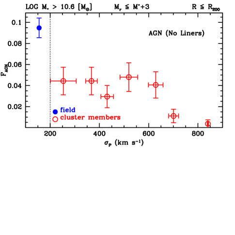
Figure 5: Relation between the AGN fraction and the velocity dispersion of the parent cluster (red open circles). The corresponding estimate for the field is indicated by the blue filled circle. The error bars indicate the 1$\sigma$ standard error on the biweight location estimate.

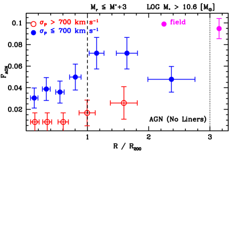
Figure 6: Variation of AGN fraction as a function of clustercentric distance for low ($\sigma_{P}\leq 700$ km s^-1) mass clusters (displayed by blue filled circles) and high mass systems ($\sigma_{P}>700$ km s^-1, red open circles). The corresponding estimate for the field is indicated by the magenta filled circle. The error bars indicate the 1$\sigma$ standard error on the biweight location estimate.

As discussed by Popesso & Biviano (2006) the anti-correlation between AGN fraction and cluster velocity dispersion may be related to the galaxy-galaxy merger inefficiency in clusters. The AGN phenomenon would be favoured in the field and low mass groups or cluster outskirts, as central cluster galaxies exhibit higher relative velocities than group galaxies or small field associations. The results from $\S$4.1.1, regarding the local environment variation, indicate the same conclusions. However, in order to reinforce that result we show in Fig. 7 the variation of the AGN fraction as a function of the normalized galaxy velocity offsets. The offsets are relative to their parent group/cluster redshift and the normalization considers the velocity dispersion of their parent system. We can see a smooth decline from the field to clusters, as galaxy velocities increase, confirming larger AGN fractions for smaller velocities. Another possible explanation for the anti-correlation between F_AGN and $\sigma_{P}$ is the environmental variation in AGN galaxy hosts, as investigated in papers III, IV and V. We tackle this issue in $\S$5.

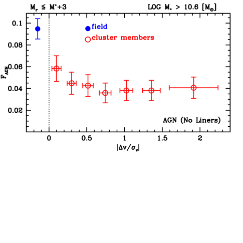
Figure 7: Variation of AGN fraction as a function of normalized relative velocities ($\Delta_{v}/\sigma_{v}$) displayed as red open circles. The corresponding estimate for the field is indicated by the blue filled circle. The error bars indicate the 1$\sigma$ standard error on the biweight location estimate.

4.2.2 Role of the Cluster Dynamical Stage

We have also investigated if the dynamical stage of the clusters plays a role in our findings (paper III). Regarding substructure we classify the clusters using the $\Delta$ (or DS) test (Dressler & Shectman, 1988) and the Hellinger Distance (HD) measure, used to detect deviations from a Gaussian velocity distribution (Ribeiro et al., 2013b). In previous works (Krause, Ribeiro & Lopes, 2013; Ribeiro et al., 2013a) we considered different tests (such as Anderson-Darling and Kolmogorov-Smirnov) of gaussianity applied to the galaxy velocity distribution. For the current work we decided to adopt the HD measure as it is the least vulnerable method to type I and II statistical errors (Ribeiro et al., 2013b). We decided to perform the substructure analysis also with the HD measure as the AGN fraction may be boosted when $\sigma_{P}$ is overestimated. In this case, a test based on galaxy velocities may be even more relevant than a 3D test (such as the DS).

In Fig. 8 we display the AGN fraction vs clustercentric distance for systems with or without substructure. In the top and bottom panels we display the results obtained with the DS and HD methods, respectively. We can see that within the virial radius (approximated by R₂₀₀) there is no difference in the results. A larger value for F_AGN for clusters with substructure can only be seen for R $>$ R₂₀₀ (especially at R $\sim$ 1.5$\times$R₂₀₀). Hence, we assume no major impact for the inclusion of systems with substructure. If the merger of subunits increases the nuclear activity in clusters the effect may be fast enough not to be detected for objects inhabiting the clusters for longer periods (those within R₂₀₀). It would be possible to detect an increase in the AGN fraction for non-relaxed clusters only for objects recent infalling, located in the clusters’ outskirts.

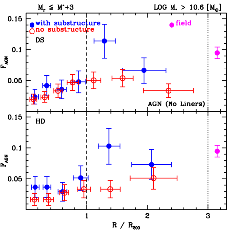
Figure 8: Relation between AGN fraction and clustercentric distance for systems with no signs of substructure (red open circles) and for which a test indicates significant substructure (blue filled circles). The corresponding estimate for the field is indicated by the magenta filled circle. In the top panel we display the results considering the DS substructure test, while in the bottom panel we exhibit the results of the HD measure. The error bars indicate the 1$\sigma$ standard error on the biweight location estimate.

5 The AGN environmental variation by galaxy type

It is well know the fraction of galaxies hosting an AGN strongly depends on galaxy morphology, as well as other parameters, such as colour and stellar mass (Choi et al., 2009; Sohn et al., 2013). Those effects may impact the environmental variation of AGN hosted by different types of galaxies. For instance, Sohn et al. (2013) find an environmental variation of the AGN fraction only when considering galactic nuclei hosted by early-types. However, it is important to emphasize their work focus mainly on the AGN population in compact groups.

In order to check the impact on galaxy morphology on our results, we make a rough separation between early and late-type galaxies, splitting galaxies according only to the concentration index (Strateva et al., 2001; Kauffmann et al., 2004; Lopes, Ribeiro & Rembold, 2014). The concentration index $C$ is defined as the ratio of the radii enclosing 90 per cent and 50 per cent of the galaxy light in the r-band, $R_{90}/R_{50}$. We simply call early-type objects (ETGs) those with C $\geq$ 2.6 and the late-type objects (LTGs) with C $<$ 2.6. Note the value of $C$ chosen to split the two populations is in good agreement to the literature (Kauffmann et al., 2004). Different values of $C$ could increase the completeness of one population, but at the cost of a higher contamination. $C=$ 2.6 represents a good compromise to split early and late type objects (see discussion in Lopes, Ribeiro & Rembold 2014). There could also be the case of transitional galaxies (such as “red discs” and “blue spheroids”), but those are rare, as investigated in Lopes et al. (2016). As our AGN sample for massive objects is small we chose not to use a more detailed separation (using several morphological types, or even more concentration index bins).

Fig. 9 display the relations derived for the AGN fractions for the ETG (top panel) and LTG (bottom panel) populations. Note that each fraction is not relative to all galaxies, as in the previous plots. Now we computed the fractions at fixed morphology, showing the number of AGN hosted by an ETG (LTG) divided by the whole ETG (LTG) population. The field value is also show as a reference. We see the environmental variation is present in both cases, although there is a large scatter for the LTG population. Hence, the AGN environmental variation we see is not an effect of the morphology-density relation. Another interesting feature in Fig. 9 is the fact the AGN fraction in the field for ETGs is larger than the cluster results, even in their outskirts. That is not the case for the LTG population, which displays a constant value from the field to R₂₀₀, decreasing inwards.

As ETGs inhabit clusters for longer periods compared to LTGs its is expected the fraction of AGN for the first population would be smaller than for the second. That is the case, if we compare the AGN fractions within R₂₀₀ for the upper and lower panels of Fig. 9. The value F_AGN hosted by LTGs is always larger than for ETGs.

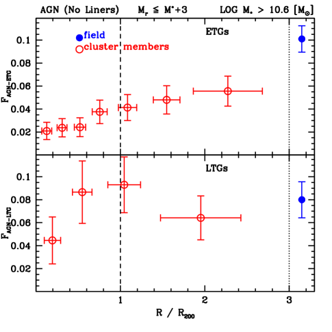
Figure 9: Relation between AGN fraction and clustercentric distance for AGN hosted by ETGs (top panel) and by LTGs (bottom panel). Those results are displayed by red open circles. The corresponding estimate for the field is indicated by the magenta filled circle. Those fractions are not relative to all galaxies. Each fraction is obtained at fixed morphology, showing the number of AGN hosted by an ETG (LTG) divided by the whole ETG (LTG) population. The error bars indicate the 1$\sigma$ standard error on the biweight location estimate.

6 The Location of AGN in phase-space

Bearing in mind the last result discussed above it is interesting to investigate the AGN distribution in phase-space (PS) and compare it to other galaxy populations. That is also important to check if an enhanced value of the AGN fractions in the cluster outskirts could be explained by galaxy interactions (Popesso & Biviano 2006; Pimbblet et al. 2013). Instead of splitting galaxies according to morphology (using concentration) we considered four types of objects according to their spectral features. As mentioned in sections 2.2 and 2.3 we adopted the spectral classification from the MPA-JHU group. In Fig. 10 we display the PS distribution of four classes, “AGN”, “Composite”, “Star Forming” and “Passive” (only massive objects, log $M_{*}>10.6$, are considered). The latter actually is composed of objects that are “Unclassifiable”. We loosely call those objects as passive, but that does not come from the spectral classification. However, there is good indication those are indeed passive, from their location in the SFR$-$M_∗ plane, as well as in the colour-colour diagram [(u-r)₀ $\times$ (r-z)₀]. The "Unclassifiable" population is consistent to passive objects, with $\gtrsim$ 99% of objects falling into the region occupied by passive galaxies on this colour-colour plot.

Visually, we infer the AGN population has different distribution than the composite, SF and passive objects. We confirm that by running a kernel density based global two-sample comparison test using the kde routine of the ks library in R. The kde test applies the so-called black-box comparisons of multivariate data (Duong, Goud & Schauer, 2012). The algorithm transforms data points into kernels and develop a multivariate two-sample test that is nonparametric and asymptotically normal to directly and quantitatively compare different distributions. The asymptotic normality bypasses the computationally intensive calculations used by the usual resampling techniques to compute the $p$-value. The complete automatic testing procedure is programmed in the ks library in R (Duong, 2007). In all two sample comparisons we perform the $p$-values of the kde test were smaller than 0.05.

On each panel the blue dashed line represents the equation proposed by Oman et al. (2013) to estimate the infall time of galaxy members ($\mid\frac{\Delta_{v}}{\sigma_{v}}\mid=-\frac{4}{3}\frac{R}{R_{vir}}+2$). As pointed out by Agulli et al. (2017) this line can be used to roughly discriminate recent ($\tau<$ 1 Gyr) and early ($\tau>$ 1 Gyr) infalls. It is clear from the figure that passive objects are a majority of early-infalls, while the SF galaxies are the opposite. The AGN and especially the composite population are a mix of early and recent infalls. At first, these results may seem hard to reconcile to the findings of Pimbblet et al. (2013), who claim no significant different between AGN and other cluster members in the phase-space (even if restricting to higher mass galaxies). However, it is worthy remember their sample is restricted to only six clusters, with no sign of substructure, while we allow the inclusion of disturbed systems. Most importantly, their sample is restricted only to massive objects, as the six clusters have $\sigma_{v}\gtrsim 800$ km s^-1. As we saw from Figs. 5 and 6 the high mass systems ($\sigma_{v}>700$ km s^-1) show much smaller AGN fractions than the lower mass objects. The variation with clustercentric distance is also much less pronounced for the massive clusters.

Considering that AGN are preferentially found outside the virial radius (R${}_{200}<$ R $<$ 1.5$\times$R₂₀₀) and display low normalized relative velocities ($\mid\Delta_{v}/\sigma_{v}\mid$) we interpret those objects may be triggered by interactions in the outskirts of groups and clusters. The AGN feedback would then be crucial for quenching SF in members of groups and clusters (Popesso & Biviano, 2006). As the velocity dispersion of the galaxy systems grows the AGN production would decrease, leading to the scenario we find today. That interpretation can also match the discussion of Pimbblet et al. (2013), who suggest that if AGN are triggered by encounters there would be enough time for them to move away from the encounter site. Hence, no interaction signs would be detected.

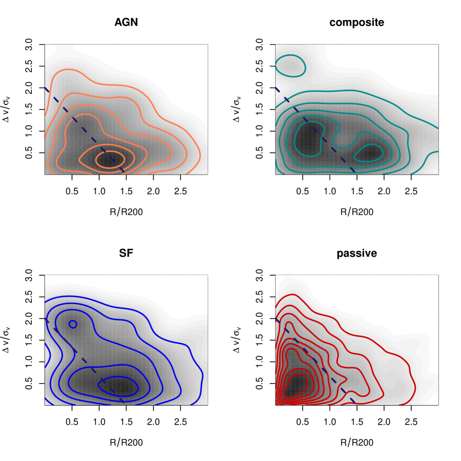
Figure 10: The phase-space distribution of AGN (top left), composite (top right), SF (bottom left), and passive (bottom right) populations. As above, only massive objects (log $M_{*}>10.6$) are considered. The blue dashed line on each panel represents the equation proposed by Oman et al. (2013) to estimate the infall time of galaxy members (see text). This line can roughly be used to separate recent and early infalls.

7 Summary

In this work we investigated the F_AGN variation with stellar mass and environment (both local and global), in the local Universe ($z\leq 0.1$). We consider cluster members, as well as a field sample in the same redshift interval. We also consider only strong AGN (no LINERs in the sample). After confirming the well know increase in the number of AGN with stellar mass we restricted our sample to the most massive objects (log $M_{*}>10.6$). The local environment is traced by the local galaxy stellar mass density and clustercentric distance, while the global environment is indicated by the cluster potential (traced by its velocity dispersion). We also searched for any dependence of the fraction of AGN on the cluster dynamical stage, and also according to galaxy type. Finally, we compare the locations of different galaxy populations in the cluster phase-space. Our main results are as follows.

1. A first indication of the importance of the global environment comes from the fact the AGN fraction, at fixed stellar mass, is typically higher in the field when compared to clusters (Fig. 2).

2. Regarding the local environment, we detect a roughly constant relation between F_AGN and local galaxy stellar mass density for field objects. However, from cluster outskirts inwards we see a steep decline in F_AGN as a function of local stellar mass density (Fig. 3).

3. A clear dependence between the AGN fraction and clustercentric distance is also detected, especially within R₂₀₀ where the variation is much stronger (Fig. 4). The field value is also larger than the cluster results, even in their outskirts.

4. We find the global environment also plays an important role as we detect a dependence on the parent cluster mass, indicated by velocity dispersion (Figs. 5 and 6). We find that F_AGN is nearly constant for $\sigma_{P}\lesssim 650-700$ km s^-1, but decreases strongly for $>$ 700 km s^-1.

5. Using two substructure tests we compared the environmental variation of clusters with and without substructure (Fig. 8). We find no significant difference within R₂₀₀ for these two cases. A larger value of the AGN fraction is only present for clusters with substructure at R $\sim$ 1.5$\times$R₂₀₀. Hence, we assume there is no major impact for using systems with substructure.

6. Using concentration to perform a rough separation between galaxy types we find the environmental variation is still detected for both types, not being an effect of the morphology-density relation (Fig. 9). However, the field AGN fraction (at fixed morphology) is larger than the cluster one, only for ETGs, being comparable to the cluster LTGs AGN fraction in the clusters outskirts.

7. When comparing AGN to other three populations in the cluster phase-space (Fig. 10) we find the AGN distribution to be significantly different than the others.

8. The AGN population is a mix of recent and early infalls, being found preferentially at R${}_{200}<$ R $<$ 1.5$\times$R₂₀₀ with low normalized relative velocities ($\mid\Delta_{v}/\sigma_{v}\mid$). We interpret the AGN phenomenon would be the result of galaxy interactions, which are favoured in the field and low mass groups or cluster outskirts, where relative velocities are typically low (see also Fig. 7).

References

- Agulli et al. (2017) Agulli I. et al. 2017, MNRAS, 467, 4410
- Alberts et al. (2016) Alberts S. et al. 2016, ApJ, 825, 72
- Alonso et al. (2007) Alonso M. Sol 2007, MNRAS, 375, 1017
- Azadi et al. (2015) Azadi M. et al. 2015, ApJ, 806, 187
- Baldwin, Phillips & Terlevich (1981) Baldwin J.A., Phillips M.M., Terlevich R. 1981, PASP, 93, 5 (BPT)
- Beers et al. (1990) Beers T.C., Flynn K., Gebhardt K. 1990, AJ, 100, 32
- Best et al. (2005) Best P. et al. 2005, MNRAS, 362, 25
- Bitsakis et al. (2015) Bitsakis T. et al. 2015, MNRAS, 450, 3114
- Brinchmann et al. (2004) Brinchmann J. et al. 2004, MNRAS, 351, 1151
- Brusa et al. (2009) Brusa M. et al. 2009, A&A, 507, 1277
- Choi et al. (2009) Choi Y. et al. 2009, ApJ, 699, 1679
- de Carvalho et al. (2017) de Carvalho R.R. et al. 2017, arXiv:1707.00651
- del Pino et al. (2017) del Pino B. et al. 2017, MNRAS, 467, 4200
- Djorgovski et al. (2003) Djorgovski S.G., de Carvalho R.R., Gal R.R., Odewahn S.C., Mahabal A.A., Brunner R.J., Lopes P.A.A., Kohl Moreira J.L. 2003, Bulletin of the Astronomical Society of Brazil, 23, 197
- Dressler & Shectman (1988) Dressler A., & Shectman S.A. 1988, AJ, 95, 985 (DS)
- Dressler et al. (1999) Dressler A. et al. 1999, ApJS, 122, 51
- Elmegreen et al. (1998) Elmegreen B. et al., 1998, ApJ, 503, L119
- Duong (2007) Duong T. 2007, Journal of Statistical Software, 21, 1
- Duong, Goud & Schauer (2012) Duong T., Goud B. & Schauer K. 2012, PNAS, 109, 8382
- Ellison et al. (2015) Ellison S.L. et al. 2015, MNRAS, 451L, 35
- Fadda et al. (1996) Fadda D., Girardi M., Giuricin G., et al. 1996, ApJ, 473, 670
- Gal et al. (2003) Gal R.R., de Carvalho R.R., Lopes P.A.A., Djorgovski S.G., Brunner R.J., Mahabal A.A., Odewahn S.C. 2003, AJ, 125, 2064
- Gal et al. (2004) Gal R.R., de Carvalho R.R., Odewahn S.C., Djorgovski S.G., Mahabal A.A., Brunner R.J., Lopes P.A.A. 2004, AJ, 128, 3082
- Gal et al. (2009) Gal R.R., Lopes P.A.A, de Carvalho R.R., Kohl-Moreira J.L., Capelato H.V., Djorgovski S.G. 2009, AJ, 137, 2981
- Genzel et al. (2008) Genzel R. et al., 2008, ApJ, 687, 59
- Goulding et al. (2014) Goulding A.D. et al. 2014, ApJ, 783, 40
- Hickox et al. (2014) Hickox R.C. et al. 2014, ApJ, 782, 9
- Kannappan (2009) Kannappan S.J. et al. 2009, AJ, 138, 579
- Kauffmann et al. (2004) Kauffmann G., White S., Heckman T. et al. 2004, MNRAS, 353, 713
- Krause, Ribeiro & Lopes (2013) Krause M.O., Ribeiro A.L.B. & Lopes P.A.A. 2013, A&A, 551, 143
- La Barbera et al. (2010) La Barbera F., Lopes P.A.A., de Carvalho R.R., de La Rosa I.G., Berlind A.A. 2010, MNRAS, 408, 1361
- Lopes et al. (2004) Lopes P.A.A., de Carvalho R.R., Gal R.R., Djorgovski S.G., Odewahn S.C., Mahabal A.A., Brunner R.J. 2004, AJ, 128, 1017
- Lopes et al. (2006) Lopes P.A.A., de Carvalho R.R., Capelato H.V., Gal R.R., Djorgovski S.G., Brunner R.J., Odewahn S.C., Mahabal A.A. 2006, ApJ, 648, 209
- Lopes (2007) Lopes P.A.A. 2007, MNRAS, 380, 1680
- Lopes et al. (2009a) Lopes P.A.A., de Carvalho R.R., Kohl-Moreira J.L., Jones C. 2009a, MNRAS, 392, 135, paper I
- Lopes et al. (2009b) Lopes P.A.A., de Carvalho R.R., Kohl-Moreira J.L., Jones C. 2009b, MNRAS, 399, 2201, paper II
- Lopes, Ribeiro & Rembold (2014) Lopes P.A.A., Ribeiro A.L.B., Rembold S.B., 2014, MNRAS, 437, 2430, paper IV
- Lopes et al. (2016) Lopes P.A.A., Rembold S.B., Ribeiro A.L.B., Nascimento R.S., Vajgel B. 2016, MNRAS, 461, 2559, paper V
- Martini et al. (2013) Martini P. et al. 2013, ApJ, 768, 1
- Miller et al. (2003) Miller C. 2003, ApJ, 597, 142
- Moore et al. (1996) Moore B. et al. 1996, Nature, 379, 613
- Muldrew et al. (2012) Muldrew S., Croton D., Skibba R. et al. 2012, MNRAS, 419, 2670
- Odewahn et al. (2004) Odewahn S.C., de Carvalho R.R., Gal R.R., Djorgovski S.G., Brunner R.J., Mahabal A.A., Lopes P.A.A., Kohl Moreira J.L., Stalder B. 2004, AJ, 128, 3092
- Oman et al. (2013) Oman K. et al. 2013, MNRAS, 431, 2307
- Pimbblet et al. (2013) Pimbblet K. et al. 2013, MNRAS, 429, 1827
- Popesso & Biviano (2006) Popesso P. & Biviano A. 2006, A&A, 460L, 23
- Ribeiro et al. (2013a) Ribeiro A.L.B., Lopes P.A.A. & Rembold S.B. 2013a, A&A, 556, 74, paper III
- Ribeiro et al. (2013b) Ribeiro A.L.B. 2013b, MNRAS, 434, 784
- Rines & Diaferio (2006) Rines K. & Diaferio A. 2006, ApJ, 132, 1275, RD06
- Sabater et al. (2015) Sabater J. et al. 2015, MNRAS, 447, 110
- Salim et al. (2007) Salim S. et al. 2007, ApJS, 173, 267
- Satyapal et al. (2014) Satyapal S. et al. 2014, MNRAS, 441, 1297
- Schawinski et al. (2010) Schawinski K. et al. 2010, ApJ, 711, 284
- Silverman et al. (2008) Silverman J.D. et al. 2008, ApJ, 679, 118
- Singh et al. (2013) Singh R. et al. 2013, A&A, 558, 43
- Sohn et al. (2013) Sohn J. et al. 2013, ApJ, 771, 106
- Springel et al. (2005) Springel V. et al., 2005, ApJ, 620, L79
- Strateva et al. (2001) Strateva I., Ivezić Z., Knapp G. et al. 2001, AJ, 122, 1861
- von der Linden et al. (2010) von der Linden A. et al. 2010, MNRAS, 404, 1231
- Wang et al. (2015) Wang L. et al. 2015, MNRAS, 449, 4476
- Yee & López-Cruz (1999) Yee H. & López-Cruz O., 1999, AJ, 117, 1985