Black hole solutions in Gauss-Bonnet-massive gravity
in the presence of power-Maxwell field

Abstract

Motivated by recent progresses in the field of massive gravity, the paper at hand investigates the thermodynamical structure of black holes with three specific generalizations: i) Gauss-Bonnet gravity which is motivated from string theory ii) PMI nonlinear electromagnetic field which is motivated from perspective of the QED correction iii) massive gravity which is motivated by obtaining the modification of standard general relativity. The exact solutions of this setup are extracted which are interpreted as black holes. In addition, thermodynamical quantities of the solutions are calculated and their critical behavior are studied. It will be shown that although massive and Gauss-Bonnet gravities are both generalizations in gravitational sector, they show opposing effects regarding the critical behavior of the black holes. Furthermore, a periodic effect on number of the phase transition is reported for variation of the nonlinearity parameter and it will be shown that for super charged black holes, system is restricted in a manner that prevents it to reach the critical point and acquires phase transition. In addition, the effects of geometrical structure on thermodynamical phase transition will be highlighted.

I Introduction

Among the generalizations of Einstein theory of the gravity, Lovelock generalization has been proven to be special one. This is due to fact that this theory enjoys the existence of several properties which include: i) This theory consists curvature-squared terms where interestingly leads to only up to quadratic order of derivation with respect to metric secondorder ; secondorderII . ii) This theory of gravity enjoys absence of ghost ghostfree . iii) This theory of gravity can solve some of the shortcomings of general relativity (GR) shortcomings . iv) This gravity arisen from the low-energy limit of heterotic string theory string . v) This theory may also play an important role in the context of the braneworld scenario braneworld . vi) It is notable that, Lovelock gravity represents a very interesting scenario to study how higher curvature corrections to black hole physics substantially change the qualitative features we know from our experience with black holes in GR.

Gauss-Bonnet (GB) theory was first introduced by Lanczos in ref. Lanczos , then rediscovered with more details by David Lovelock in ref. Lovelock . The first three terms of Lovelock gravity provide us with the well known GB gravity which consists of the cosmological constant, Einstein’s tensor and an additional term called the GB term. The first derivation of black hole solutions in the presence of GB gravity was done by Boulware and Deser in ref. secondorder . The thermodynamical properties and eikonal instability of these solutions were studied in some literatures blackholesGB . Combination of GB theory with other theories of gravity such as dilaton dilaton , rainbow rainbowI , $F(R)$ F(R) , and $F(R,G)$ F(RG)  have been done. Charged GB black hole solutions have been investigated in ref. Charged . Later, exact black hole solutions including their thermodynamical properties have been explored in ref. Therodynamics . Several generalizations of black holes with nonlinear electrodynamics have also been obtained in ref. nonlinear .

The effects of GB gravity on different properties of the system have been investigated in diverse physical contexts, to name a few: i) presentation of conserved charges of GB-AdS gravity in electric part of the Weyl tensor which gives a generalization to conformal mass definition Jatkar . ii) investigation of Holographic thermalization in GB gravity through the Wilson loop and the holographic entanglement entropy thermalization . iii) negative effects of GB parameter on superconductor phase transition through $p$-wave phase transition pwave . iv) evidences of the effects of GB gravity of bulk theory on dual conformal field theory of the boundary in AdS/CFT correspondence GBAdSCFT ; PureGB . It is worthwhile to mention that in the presence of GB gravity, gravitons are massless and they propagate with speed of light. Also, it was shown that on stationary spacetime, event horizon of black holes in the presence of GB gravity becomes Killing horizon Izumi . Some restrictions regarding the GB gravity were extracted in ref. Jose , in order to avoid violation of causality. These restrictions pointed out to requirement of an infinite tower of massive higher-spin states, as it happens in string theory veneziano , in order to complete the theory.

Recent detection of the gravitational waves from a binary black hole merger by the LIGO and Virgo collaboration has provided the possibility of testing the validation of Einstein theory of gravity Abbott . Among the future purposes of developments in detection of gravitational waves is investigation regarding the possibility of existence of massive gravitons. The GR and its generalization, GB, include the gravitons as massless particles Gupta . Whereas, in studies conducted in the context of brane-world gravity, the possible existence of the massive modes for gravity was pointed out massiveg . Massive gravity is a modification of GR based on the idea of equipping the graviton with mass. The first ghost-free theory which included massive gravitons in flat space was proposed by Fierz and Pauli in 1939 Fierz . However, it was shown by Boulware and Deser (BD) in 1972 Boulware , that there is an inevitable ghost instability in generic types of self-interactions for the massive spin-2 field of Fierz-Pauli in non-flat background. To avoid the existence of BD ghost in massive gravity, de Rham, Gabadadze and Tolley (dRGT) in 2011, introduced a set of possible interaction terms to include massive gravitons and avoid the possibility of BD ghost instability de Rham . In fact, it was shown that a subclass of massive potentials the BD ghost does not appear, both in dRGT massive gravity de RhamII and its bi-gravity extension Hinterbichler ; Living .

Black hole solutions and their thermodynamical quantities in the presence of dRGT massive theory were investigated in ref. Nieuwenhuizen . From the perspective of cosmology and astrophysics, generalization to massive gravity proved to be significantly fruitful Saridakis ; Babichev . Among its achievements in these fields one can point out: i) providing a resolution for the cosmological constant problem DvaliGS ; DvaliHK and explaining the self-acceleration of the universe without introducing the cosmological constant Deffayet ; DeffayetDG . ii) providing an equivalent massive term corresponding to a cosmological constant massivecosmologyA2 ; GratiaHW ; Kobayashi . iii) resulting into extra polarization for gravitational waves, and affecting the propagation’s speed of gravitational waves GW1 and production of gravitational waves during inflation GW2 ; GW3 .

The core stone of producing massive terms in dRGT theory is provided by employing a reference metric. Accordingly, since the reference metric plays a key role for constructing the massive theory of gravity Living , Vegh introduced a new class of massive theory Vegh . Graviton has similar behavior as lattice in holographic conductor model in this theory. Also, this theory has specific applications in the gauge/gravity duality especially in lattice physics which motivate one to use it in other frameworks as well. Considering Vegh’s massive gravity, black hole solutions, geometrical and their thermodynamical structures were obtained in ref. Vegh massiveBH . Applying this theory to a holographic superconductor with an implicit periodic potential beyond the probe limit was done and the results were in agreement with measurements on some cuprates Zeng . The modifications of TOV equation and structure of neutron stars in the context of this massive gravity were explored and shown that the maximum mass of neutron stars can be more than three times of the mass of sun NSmassive . Combination of this massive theory with gravity’s rainbow rainbow , GB gravity GBMassive and nonlinear electrodynamics were done and the modification in thermodynamical structure of the black holes were highlighted. Magnetic solutions in the presence GB-massive (non)linear electrodynamics were studied in ref. MagMassive , and it was shown that the massive terms significantly affect the singularity of deficit angle and their possible geometrical phase transitions. The existence of nonsingular universe in massive gravity’s rainbow has been investigated and pointed out in ref. nonsingular . Entropy spectrum of black holes in the presence massive gravity has been investigated in ref. Spectrum . Black hole as a heat engine within the framework of massive gravity has been studied in ref. heat engine .

Coupling of GR with nonlinear electrodynamics is a subject which attracted significant attentions because of specific properties Heisenberg . One of the interesting and special classes of the nonlinear electrodynamic is power-law Maxwell invariant (PMI) which was introduced by Hassaine and Martinez in 2007 PMI . Lagrangian of PMI is an arbitrary power of Maxwell Lagrangian PMIII , where it is invariant under the conformal transformation $g_{\mu\nu}\rightarrow\Omega^{2}g_{\mu\nu}$ and $A_{\mu}\rightarrow A_{\mu}$ ($g_{\mu\nu}$ and $A_{\mu}$ are metric tensor and the electromagnetic potential, respectively). It is notable that, when the power of Maxwell invariant is unit, this model reduces to linear Maxwell field PMIII . Another interesting property of PMI is related to its conformal invariancy. Considering power of Maxwell invariant as $s=d/4$ ($s$ and $d$ are power of PMI and dimensions of spacetime, respectively), one obtains traceless energy-momentum tensor which leads to conformal invariancy. This conformal invariancy includes Reissner-Nordström solutions which are inverse square electric field in arbitrary dimensions PMI . The black object solutions coupled to the PMI field and their thermodynamics were studied and obtained in ref. PMIresult . Also, holographic superconductors in the presence of PMI field were investigated in ref. PMIHS .

In this paper, we intend to generalize Einstein gravity action by adding GB, massive and nonlinear source to Lagrangian and obtain exact GB-Massive black holes in the presence of PMI source.

II Charged Black hole solutions in GB-Massive gravity

The $d$-dimensional action of GB-massive gravity in the presence of negative cosmological constant and power Maxwell field can be written as

$$I=-\frac{1}{16\pi}\int d^{d}x\sqrt{-g}\left[R-2\Lambda+L(F)+\alpha L_{GB}-m^{2}\sum_{i}^{4}c_{i}{}U_{i}(g,\psi)\right],$$ (1)

where $R$ is the scalar curvature, $L(F)=\left(-F\right)^{s}$ is the Lagrangian of power Maxwell theory and also $F=F_{\mu\nu}F^{\mu\nu}$ (in which $F_{\mu\nu}=\partial_{\mu}A_{\nu}-\partial_{\nu}A_{\mu}$) is the Maxwell invariant. $\alpha$ and $L_{GB}=R_{\mu\nu\gamma\delta}R^{\mu\nu\gamma\delta}-4R_{\mu\nu}R^{\mu\nu}+R^{2}$ are, respectively, the coefficient and the Lagrangian of GB gravity. $\psi$ is a fixed symmetric fiducial metric tensor. In Eq. (1), $c_{i}$ are constants and $U_{i}$’s are symmetric polynomials of the eigenvalues of the $d\times d$ matrix $K_{\nu}^{\mu}=\sqrt{g^{\mu\alpha}\psi_{\alpha\nu}}$

$$U_{1} = \left[K\right],\ \ \ \ U_{2}=\left[K\right]^{2}-\left[K^{2}\right],\ \ \ \ U_{3}=\left[K\right]^{3}-3\left[K\right]\left[K^{2}\right]+2\left[K^{3}\right],$$

$$U_{4} = \left[K\right]^{4}-6\left[K^{2}\right]\left[K\right]^{2}+8\left[K^{3}\right]\left[K\right]+3\left[K^{2}\right]^{2}-6\left[K^{4}\right],$$

$$U_{5} = \left[K\right]^{5}-10\left[K^{2}\right]\left[K\right]^{3}+20\left[K^{3}\right]\left[K\right]^{2}-20\left[K^{2}\right]\left[K^{3}\right]+15\left[K\right]\left[K^{2}\right]^{2}$$ (2)

$$-30\left[K\right]\left[K^{4}\right]+24\left[K^{5}\right],$$

$$...~{}~{}~{}.$$

Here, technically, it is not easy to study the solutions with all possible $U_{i}$’s in an arbitrary $d-$dimensions (for $i>d-2$, $U_{i}=0$). GB gravity is the general Lagrangian for $5$ and $6$ dimensions with Einstein assumptions of general relativity, and it is clear that $U_{i}=0,($i¿4$)$ for $d=6$. Although we generalize the solutions to higher dimensions, for the sake of simplicity, we keep the massive effects up to $U_{4}$. Obviously, if we regard other higher curvature terms of Lovelock theory, it is logical to consider other $U_{i}$.

We can extract the equations of motion by variation of the action (1) with respect to the metric tensor $g_{\mu\nu}$ and the Faraday tensor $F_{\mu\nu}$, so we have

$$R_{\mu\nu}-\frac{1}{2}Rg_{\mu\nu}+\Lambda g_{\mu\nu}+H_{\mu\nu}-2sF_{\mu\lambda}F_{\nu}^{\lambda}\left(-F\right)^{s-1}-\frac{1}{2}g_{\mu\nu}\left(-F\right)^{s}+m^{2}\chi_{\mu\nu}=0,$$ (3)

$$\nabla_{\mu}\left(F^{s-1}F^{\mu\nu}\right)=0,$$ (4)

where $\chi_{\mu\nu}$ and $H_{\mu\nu}$ are in the following forms

$$\chi_{\mu\nu} = -\frac{c_{1}}{2}\left(U_{1}g_{\mu\nu}-K_{\mu\nu}\right)-\frac{c_{2}}{2}\left(U_{2}g_{\mu\nu}-2U_{1}K_{\mu\nu}+2K_{\mu\nu}^{2}\right)-\frac{c_{3}}{2}\left(U_{3}g_{\mu\nu}-3U_{2}K_{\mu\nu}+6U_{1}K_{\mu\nu}^{2}-6K_{\mu\nu}^{3}\right)$$ (5)

$$-\frac{c_{4}}{2}\left(U_{4}g_{\mu\nu}-4U_{3}K_{\mu\nu}+12U_{2}K_{\mu\nu}^{2}-24U_{1}K_{\mu\nu}^{3}+24K_{\mu\nu}^{4}\right),$$

$$H_{\mu\nu} = -\frac{\alpha}{2}\left(8R^{\rho\sigma}R_{\mu\rho\nu\sigma}-4R_{\mu}^{\rho\sigma\lambda}R_{\nu\rho\sigma\lambda}-4RR_{\mu\nu}+8R_{\mu\lambda}R_{\nu}^{\lambda}+g_{\mu\nu}L_{GB}\right).$$ (6)

We consider a topological $d$-dimensional static spacetime as

$$ds^{2}=-f(r)dt^{2}+f^{-1}(r)dr^{2}+r^{2}h_{ij}dx_{i}dx_{j},\ i,j=1,2,3,...,n~{},$$ (7)

where $f(r)$ is the metric function and $h_{ij}dx_{i}dx_{j}$ is the line element of a ($d-2$)-dimensional space with constant curvature $(d-2)(d-3)k$ and volume $V_{d-2}$. We should note that the constant $k$ indicates that the boundary of $t=constant$ and $r=constant$ can be elliptic ($k=1$), flat ($k=0$) or hyperbolic ($k=-1$) curvature hypersurface.

In order to find the metric function, analytically, we should consider a suitable reference metric at the first step Vegh ; Vegh massiveBH

$$\psi_{\mu\nu}=diag(0,0,c^{2}h_{ij}),$$ (8)

where $c$ is positive constant. Using the Eq. (8), $U_{i}$’s be written as Vegh ; Vegh massiveBH

$$U_{j}=\frac{c^{j}}{r^{j}}\Pi_{k=2}^{j+1}d_{k},$$ (9)

where $d_{k}=d-k$. Using the electrical gauge potential ansatz, $A_{\mu}=h(r)\delta_{\mu}^{0}$, with Maxwell equation (4), we obtain

$$rh{{}^{\prime\prime}}(r)(2s-1)+d_{2}h{{}^{\prime}}(r)=0.$$ (10)

Using the above equation we can extract the electrical gauge potential as

$$h(r)=\left\{\begin{array}[]{cc}q,&s=0,1/2\\ \\ -q\ln\left(\frac{r}{l}\right),&s=\frac{d_{1}}{2}\\ \\ -q\sqrt{\frac{d_{2}}{2d_{3}}}r^{\frac{2s-d_{1}}{2s-1}},&otherwise\end{array}\right.,$$ (11)

where $q$ is an integration constant which is related to the electric charge. Physically, the electromagnetic gauge potential should be finite at infinity, therefore, one should impose following restriction on the nonlinearity parameter

$$\frac{2s-d_{1}}{2s-1}<0.$$ (12)

Applying the above equation, we find a restriction on the range of $s$ as

$$\frac{1}{2}<s<\frac{d_{1}}{2}.$$ (13)

To find metric function $f(r)$ for the metric (7), one may use any components of Eq. (3). For this purpose, we can use different components ($tt$ and $x_{1}x_{1}$) of Eq. (3) which can be written as

$$tt-component = \frac{d_{2}d_{3}f}{2r^{2d_{2}}}\{d_{4}d_{5}\left[m^{2}c^{4}c_{4}+\alpha f^{2}\right]r^{2d_{4}}+d_{4}\left[m^{2}c^{3}c_{3}+2\alpha ff{{}^{\prime}}\right]r^{2d_{7/2}}+\left[m^{2}c^{2}c_{2}-f\right]r^{2d_{3}}$$ (14)

$$+\frac{\left[m^{2}cc_{1}-f{{}^{\prime}}\right]r^{2d_{5/2}}}{d_{3}}-\frac{2\Lambda r^{2d_{2}}}{d_{2}d_{3}}-r^{2d_{3}}k\left(\alpha d_{4}d_{5}\left[2f-k\right]r^{-2}+2\alpha d_{4}f^{\prime}r^{-1}-1\right)\}+\Phi_{1},$$

$$x_{1}x_{1}-component = \frac{-d_{3}d_{4}}{2r^{2d_{3}}}\{d_{5}d_{6}\left[m^{2}c^{4}c_{4}+\alpha f^{2}\right]r^{2d_{4}}+d_{5}\left[m^{2}c^{3}c_{3}+4\alpha ff{{}^{\prime}}\right]r^{2d_{7/2}}-\frac{\left(2\Lambda+f{{}^{\prime\prime}}\right)r^{2d_{2}}}{d_{3}d_{4}}$$ (15)

$$+\left[m^{2}c^{2}c_{2}+2\alpha f{{}^{\prime 2}+2\alpha f}f{{}^{\prime\prime}}-f\right]r^{2d_{3}}+\frac{\left[m^{2}cc_{1}-2f{{}^{\prime}}\right]r^{2d_{5/2}}}{d_{4}}$$

$$-r^{2d_{3}}k\left(\alpha d_{5}d_{6}\left[2f-k\right]r^{-2}+4\alpha d_{5}f^{\prime}r^{-1}+2\alpha f^{\prime\prime}-1\right)\}+\Phi_{2}.$$

where $\Phi_{1}$ and $\Phi_{2}$ are, respectively,

$$\Phi_{1} = \left\{\begin{array}[]{cc}0&s=0,1/2\\ \\ -\left(2\right)^{\frac{d_{3}}{2}}d_{2}f\left(\frac{q}{r}\right)^{d_{1}},&s=\frac{d_{1}}{2}\\ \\ -\frac{\left(2s-1\right)f}{2}\left(\frac{d_{2}q^{2}\left(2s-d_{1}\right)^{2}}{d_{3}\left(2s-1\right)^{2}}r^{\frac{-2d_{2}}{2s-1}}\right)^{s},&otherwise\end{array}\right.,$$ (21)

$$\Phi_{2} = \left\{\begin{array}[]{cc}0&s=0,1/2\\ \\ -2\left(2\right)^{\frac{d_{5}}{2}}\frac{q^{d_{1}}}{r^{d_{3}}},&s=\frac{d_{1}}{2}\\ \\ -\frac{r^{2}}{2}\left(\frac{d_{2}q^{2}\left(2s-d_{1}\right)^{2}}{d_{3}\left(2s-1\right)^{2}}r^{\frac{-2d_{2}}{2s-1}}\right)^{s},&otherwise\end{array}\right..$$ (29)

Now, by using the Eqs. (14) and (15), we can obtain the metric function as

$$f\left(r\right) = k+\frac{r^{2}}{2\alpha d_{3}d_{4}}\left\{1-\sqrt{1+\frac{4\alpha d_{3}d_{4}}{d_{2}}\left[\frac{2\Lambda}{d_{1}}+\frac{d_{2}m_{0}}{r^{d_{1}}}+\Gamma\left(r\right)+\Upsilon\right]}\right\},$$ (30)

$$\Upsilon = -m^{2}d_{2}\left[\frac{d_{3}d_{4}c^{4}c_{4}}{r^{4}}+\frac{d_{3}c^{3}c_{3}}{r^{3}}+\frac{c^{2}c_{2}}{r^{2}}+\frac{cc_{1}}{d_{2}r}\right],$$ (31)

$$\Gamma\left(r\right) = \left\{\begin{array}[]{cc}0&s=0,1/2\\ \\ 2^{d_{1}/2}d_{2}\left(\frac{q}{r}\right)^{d_{1}}\ln\left(\frac{r}{l}\right),&s=\frac{d_{1}}{2}\\ \\ \frac{\left(2s-1\right)^{2}}{2s-d_{1}}\left(\frac{d_{2}q^{2}\left(2s-d_{1}\right)^{2}}{d_{3}\left(2s-1\right)^{2}}r^{\frac{-2d_{2}}{2s-1}}\right)^{s}&otherwise\end{array}\right..$$ (37)

In the above equation, $m_{0}$ is integration constants which is related to the total mass of the black hole. It is notable that, obtained solutions (30), satisfy all components of Eq. (3).

Here, we want to study the existence of the singularity for obtained solutions. To find that, we investigate the Kretschmann scalar. Straightforward calculations show that the Kretschmann scalar for small values leads to

$${\lim_{r\longrightarrow 0}}R_{\alpha\beta\gamma\delta}R^{\alpha\beta\gamma\delta}=\infty,$$ (38)

so, there is an essential singularity located at the origin ($r=0$). In order to study asymptotical behavior of the metric solutions, one can investigate the Kretschmann scalar for large values of radial coordinate. We find it as

$${\lim_{r\longrightarrow\infty}}R_{\alpha\beta\gamma\delta}R^{\alpha\beta\gamma\delta}=\frac{\left[d_{-1}d_{1}d_{2}+\left(4\Lambda d_{-1}+d_{1}\right)\alpha d_{3}d_{4}\right]d_{2}-\left(d_{-1}d_{2}+d_{3}d_{4}\alpha\right)\sqrt{d_{1}d_{2}\left[8d_{3}d_{4}\alpha\Lambda+d_{1}d_{2}\right]}}{d_{1}d_{2}d_{3}^{2}d_{4}^{2}\alpha^{2}}.$$ (39)

Also for small values of GB parameter it will yield

$${\lim_{\alpha\longrightarrow 0}}R_{\alpha\beta\gamma\delta}R^{\alpha\beta\gamma\delta}=\frac{8d_{-1}}{d_{1}^{2}d_{2}}\Lambda^{2}-\frac{4}{d_{1}d_{2}}\Lambda+O\left(\alpha\right).$$ (40)

The above equations (Eqs. (39) and (40)), confirm that asymptotical behavior of the solutions is (A)dS with an effective cosmological constant $\Lambda_{eff}=\Lambda_{eff}(\Lambda,\alpha)$. Therefore, the solution (30), describes a $d$-dimensional asymptotically (A)dS topological black hole with a negative, zero or positive constant curvature hypersurface in GB-massive gravity in the presence of power Maxwell field.

Also, in the absence of massive parameter ($m=0$), the solution (30) reduces to the obtained metric function for GB gravity in the presence power Maxwell field GBPMI

$$f\left(r\right)=k+\frac{r^{2}}{2\alpha d_{3}d_{4}}\left\{1-\sqrt{1+\frac{4\alpha d_{3}d_{4}}{d_{2}}\left[\frac{2\Lambda}{d_{1}}+\frac{d_{2}m_{0}}{r^{d_{1}}}+\Gamma\left(r\right)+\Upsilon\right]}\right\}.$$ (41)

The existence of at least one horizon for the obtained metric function shows that these solutions may be interpreted as black hole solutions. Considering the specific values of different parameters of massive gravity, the metric function will have two different cases; i) the usual behavior similar to GB-Maxwell gravity (two horizons, or one extreme horizon, or no horizon (naked singularity), see Figs. 1 and 2, for more details). ii) the existence of more than two roots for the metric function. In other words, we encounter with interesting solutions which have two normal and one extreme (outer) horizons or four horizons (see Figs.1 and 2, for more details). In other words, the massive parameters affect the number of roots of the metric function.

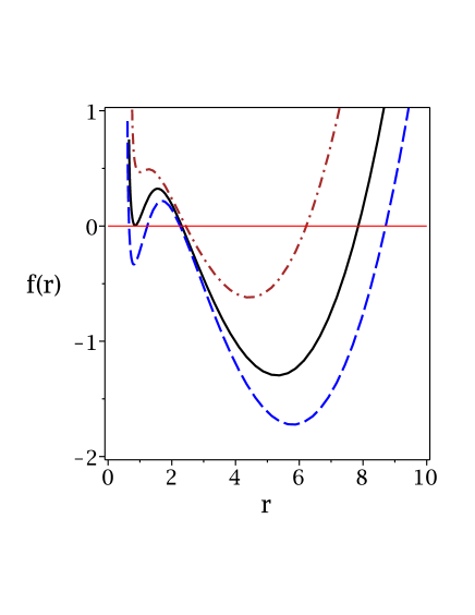
Figure 1: $f(r)$ versus $r$ for $\Lambda=-1$, $q=1$, $\alpha=1.4$, $m=2$, $c_{1}=-0.8$, $c_{2}=-0.5$, $c_{3}=1$, $c_{4}=-0.8$, $s=0.7$, $m_{0}=0.4$, $k=1$, $d=5$, $c=1.00$ (dashed-dotted line), $c=1.19$ (continues line) and $c=1.30$ (dashed line).

$\begin{array}[]{cc}\epsfbox{frdiffs1.eps}&\epsfbox{frdiffs2.eps}\end{array}$

Figure 2: $f(r)$ versus $r$ for $\Lambda=-1.2$, $q=1$, $\alpha=0.4$, $m=2$, $c=1.1$, $c_{1}=-0.8$, $c_{2}=-0.35$, $c_{3}=1$, $c_{4}=-0.8$, $m_{0}=0.4$, $k=1$, $d=5$, $s=0.55$ (bold dashed-dotted line), $s=0.68$ (bold continues line), $s=0.80$ (bold dotted line), $s=0.9$ (dotted line), $s=0.93$ (continues line) and $s=0.98$ (dashed-dotted line).

III Thermodynamics

In order to investigate the first law of thermodynamics, first, we calculate the conserved and thermodynamics quantities of the static black hole solutions in $d$-dimensional GB-massive context, and then by using these quantities we examine the first law of thermodynamics.

Applying the definition of surface gravity at the outer horizon $r_{+}$, we obtain the Hawking temperature of this black hole in the following form

$$T = \frac{1}{4\pi r_{+}\left[r_{+}^{2}+2\alpha kd_{3}d_{4}\right]}\left\{\Xi_{1}+d_{3}k\left(\alpha d_{4}d_{5}k+r_{+}^{2}\right)-\frac{r_{+}^{4}}{d_{2}}\left(2\Lambda+\Xi_{2}\right)\right\},$$ (42)

where $\Xi_{1}$ and $\Xi_{2}$ are, respectively, the massive and PMI effects on the temperature with the following explicit forms

$$\Xi_{1} = m^{2}\left(cc_{1}r_{+}^{3}+d_{3}c^{2}c_{2}r_{+}^{2}+d_{3}d_{4}c^{3}c_{3}r_{+}+d_{3}d_{4}d_{5}c^{4}c_{4}\right),$$ (44)

$$\Xi_{2} = \left\{\begin{array}[]{cc}d_{2}2^{\frac{d_{1}}{2}}\left(\frac{q}{r_{+}}\right)^{d_{1}},&s=\frac{d_{1}}{2}\\ \left(1-2s\right)\left(\frac{d_{2}q^{2}\left(d_{1}-2s\right)^{2}}{d_{3}\left(2s-1\right)^{2}}r_{+}^{\frac{-2d_{2}}{2s-1}}\right)^{s},&otherwise\end{array}\right..$$ (47)

We use the flux of the electromagnetic field at infinity to calculate the electric charge of the black hole, yielding

$$Q=\left\{\begin{array}[]{cc}-\frac{2^{d_{9}/2}d_{1}}{\pi}q^{d_{2}},&s=\frac{d_{1}}{2}\\ \frac{s\left(2s-1\right)q^{2s-1}}{2^{7/2}\pi\sqrt{\frac{d_{2}}{d_{3}}}\left(d_{1}-2s\right)}\left(\frac{d_{2}\left(d_{1}-2s\right)^{2}}{d_{3}\left(2s-1\right)^{2}}\right)^{s},&otherwise\end{array}\right..$$ (48)

Next, we use the definition introduced in ref. blackholesGB for calculating the electric potential, $U$, as

$$U=A_{\mu}\chi^{\mu}\left|{}_{r\rightarrow reference}\right.-A_{\mu}\chi^{\mu}\left|{}_{r\rightarrow r_{+}}\right.=\left\{\begin{array}[]{cc}q\ln\left(\frac{r_{+}}{l}\right)&s=\frac{d_{1}}{2}\\ &\\ q\sqrt{\frac{d_{2}}{2d_{3}}}r_{+}^{\frac{2s-d_{1}}{2s-1}},&otherwise\end{array}\right..$$ (49)

Due to generalization of Einstein gravity to GB gravity, one can use Wald’s formula to obtain the entropy of the black holes blackholesGB . This leads to

$$S=\frac{V_{d_{2}}}{4}r_{+}^{d_{2}}\left(1+\frac{2d_{2}d_{3}}{r_{+}^{2}}k\alpha\right).$$ (50)

It is notable that, the above equation shows that the area law is violated for the GB black holes with non-flat horizons.

Another important conserved quantity is the total mass of black holes. For finding it, one can use the Hamiltonian approach which results into

$$M=\frac{V_{d_{2}}\ d_{2}\ m_{0}}{16\pi}.$$ (51)

Now, we define the intensive parameters conjugating to $S$ and $Q$. These quantities are the temperature and the electric potential with the following form

$$T=\left(\frac{\partial M}{\partial S}\right)_{Q}\ \ \ \ \ \ \ \&\ \ \ \ \ \ \ \ U=\left(\frac{\partial M}{\partial Q}\right)_{S}.$$ (52)

The above results coincide with Eqs. (42) and (49) and, therefore, we find that these conserved and thermodynamic quantities satisfy the first law of black hole thermodynamics as

$$dM=TdS+UdQ.$$ (53)

IV Heat capacity

The heat capacity is one of the thermodynamical quantities carrying crucial information regarding thermodynamical structure of the black holes. There are three specific information that are of interest regarding heat capacity: i) the discontinuities of this quantity mark the possible thermal phase transitions that system can undergo. ii) the sign of it determines whether the system is thermally stable or not. In other words, the positivity corresponds to thermal stability while the opposite shows instability. iii) the roots of this quantity are also of interest since it may yield the possible changes between stable/instable states or bound point. Due to these important points, this section and the following one are dedicated to calculation of the heat capacity of the solutions and investigation of thermal structure of the black holes using such quantity. We will show that by using this quantity alongside of the temperature, we can draw a picture regarding the possible thermodynamical phase structures of these black holes and stability/instability that these black holes could enjoy/suffer.

One can use following relation for calculating the heat capacity

$$C_{Q}=\frac{T}{\left(\frac{\partial^{2}M}{\partial S^{2}}\right)_{Q}}=T(r_{+})\left(\frac{\partial S(r_{+})}{\partial T(r_{+})}\right)_{Q}=T\frac{\left(\frac{\partial S}{\partial r_{+}}\right)_{Q}}{\left(\frac{\partial T}{\partial r_{+}}\right)_{Q}}.$$ (54)

IV.1 Special case: $s=\frac{d_{1}}{2}$:

Considering Eqs. (42) and (50) for the case $s=\frac{d_{1}}{2}$, we can obtain the heat capacity in the following form

$$C_{Q}=\frac{B_{1}}{C_{1}},$$ (55)

in which $B_{1}$ and $C_{1}$ are

$$B_{1} = -\frac{d_{2}^{2}r_{+}^{d_{2}}}{2}\left(d_{3}d_{4}\alpha k\left[d_{3}d_{4}\alpha k+r_{+}^{2}\right]+\frac{r_{+}^{4}}{4}\right)\left[d_{3}k\left[d_{4}d_{5}\alpha k+r_{+}^{2}\right]+\Xi_{1_{+}}-\frac{r_{+}^{4}}{d_{2}}\left(2\Lambda+2^{\frac{d_{1}}{2}}\left(\frac{q}{r_{+}}\right)^{d_{1}}\right)\right],$$ (56)

$$C_{1} = r_{+}^{2}\left\{d_{2}d_{3}d_{4}\alpha k^{2}\left[d_{3}d_{4}d_{5}\alpha k+\frac{d_{9}r_{+}^{2}}{2}\right]+k\left(d_{3}d_{4}\alpha r_{+}^{4}\left[6\Lambda-d_{2}d_{4}2^{\frac{d_{1}}{2}}\left(\frac{q}{r_{+}}\right)^{d_{1}}+\frac{d_{2}}{2d_{4}\alpha}\right]\right.\right.$$ (57)

$$\left.-m^{2}d_{2}d_{3}d_{4}\alpha\left[2cc_{1}r_{+}^{3}+d_{3}c^{2}c_{2}r_{+}^{2}+d_{3}d_{4}d_{5}c^{4}c_{4}\right]\right)+\frac{m^{2}d_{2}d_{3}r_{+}^{2}}{2}\left[c^{2}c_{2}r_{+}^{2}+2d_{4}c^{3}c_{3}r_{+}+3d_{4}d_{5}c^{4}c_{4}\right]$$

$$\left.+r_{+}^{6}\left(\Lambda-\frac{2^{\frac{d_{1}}{2}}d_{2}^{2}}{2}\left(\frac{q}{r_{+}}\right)^{d_{1}}\right)\right\},$$

and also $\Xi_{1_{+}}=\Xi_{1_{\left|{}_{r=r_{+}}\right.}}$.

IV.2 general case: $s\neq\frac{d_{1}}{2}$:

Considering Eqs. (42) and (50) for case $s\neq\frac{d_{1}}{2}$, we can obtain the heat capacity

$$C_{Q}=\frac{B_{2}}{C_{2}},$$ (58)

where $B_{2}$ and $C_{2}$ are

$$B_{2} = -\frac{d_{2}^{2}r_{+}^{d_{2}}}{2}\left(d_{3}d_{4}\alpha k\left[d_{3}d_{4}\alpha k+r_{+}^{2}\right]+\frac{r_{+}^{4}}{4}\right)\left[d_{3}k\left[d_{4}d_{5}\alpha k+r_{+}^{2}\right]+\Xi_{1_{+}}-\frac{r_{+}^{4}}{d_{2}}\left(2\Lambda+\frac{\Xi_{2_{+}}}{\left(1-2s\right)}\right)\right],$$ (59)

$$C_{2} = r_{+}^{2}\left\{d_{2}d_{3}d_{4}\alpha k^{2}\left[d_{3}d_{4}d_{5}\alpha k+\frac{d_{9}r_{+}^{2}}{2}\right]+k\left(d_{3}d_{4}\alpha r_{+}^{4}\left[6\Lambda-\frac{\left(2ds-10s+3\right)\Xi_{2_{+}}}{\left(1-2s\right)}+\frac{d_{2}}{2d_{4}\alpha}\right]\right.\right.$$ (60)

$$\left.-m^{2}d_{2}d_{3}d_{4}\alpha\left[2cc_{1}r_{+}^{3}+d_{3}c^{2}c_{2}r_{+}^{2}+d_{3}d_{4}d_{5}c^{4}c_{4}\right]\right)+\frac{m^{2}d_{2}d_{3}r_{+}^{2}}{2}\left[c^{2}c_{2}r_{+}^{2}+2d_{4}c^{3}c_{3}r_{+}+3d_{4}d_{5}c^{4}c_{4}\right]$$

$$\left.+r_{+}^{6}\left(\Lambda-\frac{\left(2ds-6s+1\right)\Xi_{2_{+}}}{2\left(2s-1\right)^{2}}\right)\right\},$$

and also $\Xi_{2_{+}}=\Xi_{2_{\left|{}_{r=r_{+}}\right.}}$.

V Results, discussion and conclusion

Unfortunately, it was not possible to obtain divergence points and roots of the heat capacity analytically, and therefore, we employed the numerical method. In order to investigate the effects of different factors on thermodynamical behavior of the solutions, we have plotted following diagrams for variation of the gravitons’s mass (Fig. 3), GB factor (Fig. 4), nonlinear parameter (Fig. 5), electric charge (Fig. 6) and topological factor (Fig. 7).

The heat capacity provided in this paper could enjoy one of the following cases: i) one root and being an increasing function of the horizon radius. ii) one root with one divergency. iii) one root and two divergencies. Correspondingly, the temperature enjoys one of the following behaviors: i) having one root. ii) existence of one root and one extremum. iii) having one root, one maximum and one minimum. iv) existence of one root, one divergency and one minimum which is reported only for black holes with hyperbolic horizon. The root of temperature is coincidence with the root of heat capacity, except for one case that will be highlighted later. The divergencies of heat capacity are taking place exactly where temperature acquires an extremum. Before the root, both heat capacity and temperature are negative which indicate non-physical unstable solutions. The divergencies of heat capacity take place only after root. If there is only one divergency, heat capacity is positive around it, so the solutions are thermally stable. In this case, our thermodynamical system meets a critical point at where heat capacity diverges. In the case of two divergencies, between root and smaller divergence point and after larger divergency, since heat capacity is positive valued, the solutions are thermally stable in these regions. Between the divergencies, heat capacity is negative indicating unstable state. This shows that for this case, a phase transition takes place between divergencies.

$\begin{array}[]{cc}\epsfbox{T-M.eps}&\epsfbox{C-M.eps}\end{array}$

Figure 3: $T$ (left panel) and $C$ (right panel) versus $r_{+}$ for $\Lambda=-1$, $q=1$, $\alpha=0.5$, $c=c_{1}=c_{2}=c_{3}=2$, $c_{4}=1$, $k=1$, $d=5$, $s=0.7$, $m=0$ (continuous line), $m=0.35$ (dotted line), $m=0.4138$ (dashed line) and $m=0.5$ (dashed-dotted line).

$\begin{array}[]{cc}\epsfbox{T-alpha.eps}&\epsfbox{C-alpha.eps}\end{array}$

Figure 4: $T$ (left panel) and $C$ (right panel) versus $r_{+}$ for $\Lambda=-1$, $q=1$, $m=0.4$, $c=c_{1}=c_{2}=c_{3}=2$, $c_{4}=1$, $k=1$, $d=5$, $s=0.7$, $\alpha=0$ (continuous line), $\alpha=0.4$ (dotted line), $\alpha=0.479$ (dashed line) and $\alpha=0.5$ (dashed-dotted line).

$\begin{array}[]{cc}\epsfbox{T-S-1.eps}&\epsfbox{C-S-1.eps}\\ \epsfbox{T-S-2.eps}&\epsfbox{C-S-2.eps}\\ \epsfbox{T-S-3.eps}&\epsfbox{C-S-3.eps}\end{array}$

Figure 5: $T$ (left panel) and $C$ (right panel) versus $r_{+}$ for $\Lambda=-1$, $q=1$, $m=0.4$, $c=c_{1}=c_{2}=c_{3}=2$, $c_{4}=1$, $k=1$, $d=5$, $\alpha=0.5$.
Up panels: $s=0.6$ (continuous line), $s=0.61$ (dotted line), $s=0.6205$ (dashed line) and $s=0.63$ (dashed-dotted line).
Middle panels: $s=1.2$ (continuous line), $s=1.4$ (dotted line), $s=1.56$ (dashed line) and $s=1.8$ (dashed-dotted line).
Down panels: $s=1.9$ (continuous line), $s=3.2$ (dotted line), $s=3.64$ (dashed line) and $s=4$ (dashed-dotted line).

$\begin{array}[]{cc}\epsfbox{T-q.eps}&\epsfbox{C-q.eps}\end{array}$

Figure 6: $T$ (left panel) and $C$ (right panel) versus $r_{+}$ for $\Lambda=-1$, $\alpha=0.5$, $m=0.4$, $c=c_{1}=c_{2}=c_{3}=2$, $c_{4}=1$, $k=1$, $d=5$, $s=0.7$, $q=0$ (continuous line), $q=0.2$ (dotted line), $q=0.24$ (dashed line) and $q=0.3$ (dashed-dotted line).

$\begin{array}[]{ccc}\epsfbox{T-k.eps}&\epsfbox{C-k.eps}&\epsfbox{CT-k.eps}\end{array}$

Figure 7: For $\Lambda=-1$, $q=1$, $m=0.4$, $c=c_{1}=c_{2}=c_{3}=2$, $c_{4}=1$, $\alpha=0.4$, $d=5$, $s=0.7$, $k=1$ (continuous line), $k=0$ (dotted line) and $k=-1$ (dashed line).
$T$ (left panel) and $C$ (middle panel) versus $r_{+}$. Right panel: $T$ (continuous line) and $C$ (dashed line) versus $r_{+}$ for $k=-1$.

Evidently, for small values of the massive parameter, the heat capacity enjoys only one root. The place of root is a decreasing function of this parameter. Increasing massive gravity results into formation of divergencies in the structure of heat capacity. Therefore, for sufficiently large values of the massive parameter, thermodynamical system acquires critical behavior and phase transition (see Fig. 3). The effects of GB parameter are opposite to massive parameter. In other words, by increasing the value of this parameter, the divergencies of heat capacity, hence phase transitions in thermal structure of the heat capacity are omitted (Fig. 4). The effects of nonlinearity parameter proves to be outstanding. Increasing this parameter results into periodic behavior for existence of divergencies and their number. For specific region, increasing the nonlinearity parameter results into vanishing the divergencies, and heat capacity becomes a smooth function of the horizon radius (see up panels of Fig. 5). Interestingly, increasing the nonlinearity further causes the heat capacity to acquire the divergencies that were omitted (see middle panels of Fig. 5). Therefore, system will have thermodynamically critical behavior. But, if the nonlinearity parameter is increased again, the divergencies will vanish again (see down panels of Fig. 5). Therefore, we observe a periodic behavior for existence/absence of thermodynamical phase transition for the black holes for variation of the nonlinearity parameter. This specific behavior is solely belongs to this type of the nonlinear electromagnetic field and Born-Infeld families of the nonlinear electromagnetic field do not possess such property. The effects of variation of electric charge is depicted in Fig. 6. Interestingly, in the absence of electric charge, the temperature and heat capacity acquires a non-zero value for vanishing horizon radius (see continuous line in Fig. 6). Considering this specific behavior and evaporation of the black holes mechanism, one can point out that for these black holes, in evaporation process (where horizon radius is vanished) a trace of existence of the black holes is left in term of thermal fluctuation. This is a generic behavior that is present for the black holes due to massive gravity generalization. Previously, existence of the trace of thermal fluctuation for temperature of the black holes in the presence of massive gravity was reported for $3$ and $4$ dimensional black holes. Presence of it in $5$ dimensional case signals that this is a generic behavior available for black holes in massive gravity generalization. Existence of such trace could be used to address the long standing issue of information paradox for black holes. As we can see, for non-zero value of the electric charge, this specific behavior is omitted and, temperature and heat capacity acquire a root. For the absence or small values of the electric charge, heat capacity enjoys the presence of two divergencies in its structure. Increasing the value of electric charge results into first one divergency and then its vanishing. This shows the number of the divergencies is a decreasing function of the electric charge. Finally, as one can see, the topological factor, modifies the place of divergencies in heat capacity and their number as well (Fig. 7). One of the most interesting results is regarding black holes with hyperbolic horizon. For this specific horizon, temperature enjoys a root, a divergency and one minimum in its structure. Before the root and after the divergency, temperature is positive valued whereas between root and divergency, temperature is negative, therefore solutions are nonphysical. Interestingly, the divergency of temperature is coincided with an extremum root in the heat capacity (see right panel of Fig. 7). For $k=-1$, the root of temperature coincides with a non-extremum root in the heat capacity and extremum of the temperature is matched with a divergency in the heat capacity. Before the root of temperature, both temperature and heat capacity are positive valued indicating existence of physical stable state. Between the root and divergency of the temperature, both heat capacity and temperature are negative valued, hence solutions are not physical. Between divergency of the temperature and its minimum, temperature is positive whereas, interestingly, heat capacity is negative valued indicating the existence of physical unstable state for black holes. After the minimum of temperature (divergency of heat capacity), both temperature and heat capacity are positive. This shows that there is a phase transition between medium unstable black holes and larger stable ones. If one compare the hyperbolic case with spherical/flat black holes, one can see that thermodynamically speaking, there are significant differences between the thermodynamical structure and phase transitions of black holes in these two horizons. On the other hand, as we can see, not all the roots in heat capacity are matched with roots in the temperature. Interestingly, as we study the heat capacity, no discontinuity is observed where temperature is divergent. This shows the necessity of investigating temperature and heat capacity separately and also together to draw a better picture regarding the thermodynamical behavior of the black holes.

The nonzero massive parameter is related to the mass of gravitons. As we can see, the increment in this parameter results into system acquiring a critical thermodynamical behavior. Depending on the values of $m$, system may acquire specific critical behavior. Recently, it was pointed out that quasi normal modes of the black holes present a characteristic behavior in their frequencies which exactly takes place where system has a thermodynamical phase transition. Considering this fact, the specific contributions of the massive gravity into thermodynamical structure of the black holes could be employed to distinguish the validity of massive gravity generalization. As for the GB gravity, studying the Ricci scalar or Riemann tensor shows that the effects of GB gravity is toward increasing the value of these quantities. Increment in the value of curvature scalar indicates stronger gravitational power. Therefore, on can conclude that strength of the gravitational field is an increasing function of the GB parameter. Considering this fact, we can see that by increasing the value of GB parameter, hence the strong gravitational field, the critical behavior is omitted. This shows that the presence of an instability, hence a phase transition, is more probable to be seen in black holes with weaker gravitational field, the existence of a phase transition is less possible or even in some cases impossible. This shows that as we increase the strength of gravitational field, a rearrange in thermodynamical distribution of the system is done in a manner to avoid thermal phase transition. This also shows that gravitational strength and, thermodynamical behavior and properties are closely related and the modification in one has more direct and observable effects on the other one. The topological factor represents the geometrical structure of the horizon for black holes provided in this paper. As we have pointed out, depending on the type of horizon, thermodynamical structure of the black holes would be significantly different. This signals us with the fact that geometrical structure of our object of interest also plays a crucial role in determining the thermodynamical behavior of it. Therefore, one can conclude that there is also a direct relation between thermodynamical properties of the system (including phase transitions), and geometrical structure. In essence, we are expecting this fact. The reason is because through Einstein point of the view of gravity, gravity is induced due to geometrical variation of the spacetime. Such variation is originated from the effects of mass on the spacetime. Therefore, there is a direct relation between gravitational field and geometrical properties. Establishing the fact that gravitational field directly affects the thermodynamical behavior, one can conclude that there is a direct relation between geometrical structure and thermodynamical properties. In our study of the heat capacity, such link between geometrical properties and thermodynamical behavior was highlighted. This signals us with the fact that the origin of thermodynamical behavior, geometrical structure and gravitational field could be the same. In the context of electric charge, we observed that increasing electric charge results into omitting the divergencies in the heat capacity. One can conclude that for super charged black holes, system is restricted in a manner that prevents the thermodynamical structure reaching critical behavior. This shows that the total net charge provided for black holes could modify the structure of black holes to a level of canceling the effects of the massive gravity and GB generalization. Comparing to other generalizations, the electric charge is of a more free nature. This is due to fact that black holes by consuming the matters surrounding them, can achieve higher values of the electric charge. This shows that comparing to other parameters discussed in the paper, the electric charge could grow more rapidly comparing to other factors considered and discussed before. Once more, we point out that in the absence of electric field, the generalization to massive gravity provided black holes with a possibility of existence of non-zero temperature and heat capacity for vanishing horizon radius. This indicates the presence of a trace of existence of black holes even after black hole evaporation. This is a generic property which so far was observed only for black holes in the presence of massive gravity. Finally, the periodic effect of nonlinearity parameter on the existence of divergencies in heat capacity, hence phase transition should be pointed out. The nonlinearity parameter measures the degree of nonlinear nature of the electromagnetic field. In the context of Born-Infeld family of nonlinear electromagnetic fields, increasing the nonlinearity parameter results into decreasing the nonlinear nature of the electromagnetic field. In other words, for large values of the nonlinearity parameter, electromagnetic field in Born-Infeld family will yield a Maxwell-like behavior. Interestingly, for PMI case, the Maxwell-like case is achieved for only a specific case ($s=1$) and variation of the nonlinearity parameter results into periodic behavior regarding the existence of phase transition points. This shows that PMI theory enjoys the larger number of the possibilities regarding existence of the critical behavior comparing to Born-Infeld theories.

- (1) D. G. Boulware and S. Deser, Phys. Rev. Lett. 55, 2656 (1985).
- (2) B. Zumino, Phys. Rept. 137, 109 (1986); J. T. Wheeler, Nucl. Phys. B 268, 737 (1986).
- (3) R. Myers, Nucl. Phys. B 289, 701 (1987); C. Callan, R. Myers and M. Perry, Nucl. Phys. B 311, 673 (1989).
- (4) K. S. Stelle, Gen. Rel. Grav. 9, 353 (1978); W. Maluf, Gen. Rel. Grav. 19, 57 (1987); M. Farhoudi, Gen. Rel. Grav. 38, 1261 (2006).
- (5) B. Zwiebach, Phys. Lett. B 156, 315 (1985); D. J. Gross and E. Witten, Nucl. Phys. B 277, 1 (1986); R. R. Metsaev and A. A. Tseytlin, Phys. Lett. B 191, 354 (1987).
- (6) N. Deruelle and T. Dolezel, Phys. Rev. D 62, 103502 (2000); C. Charmousis and J. F. Dufaux, Class. Quantum Grav. 19, 4671 (2002); S. C. Davis, Phys. Rev. D 67, 024030 (2003); J. P. Gregory and A.Padilla, Class. Quantum Grav. 20, 4221 (2003).
- (7) C. Lanczos, Ann. Math. 39, 842 (1938).
- (8) D. Lovelock, J. Math. Phys. 12, 498 (1971); D. Lovelock, J. Math. Phys. 13, 874 (1972).
- (9) J. E. Kim, B. Kyae and H. M. Lee, Phys. Rev. D 62, 045013 (2000); Y. M. Cho and I. P. Neupane, Phys. Rev. D 66, 024044 (2002); C. Charmousis and J. -F. Dufaux, Class. Quantum Grav. 19, 4671 (2002); R. -G. Cai, Phys. Rev. D 65, 084014 (2002); G. Kofinas, R. Maartens and E. Papantonopoulos, JHEP 10, 066 (2003); R. G. Cai and Q. Guo, Phys. Rev. D 69, 104025 (2004); A. Barrau, J. Grain and S. O. Alexeyev, Phys. Lett. B 584, 114 (2004); K. -i. Maeda and T. Torii, Phys. Rev. D 69, 024002 (2004); C. de Rham and A. J. Tolley, JCAP 07, 004 (2006); G. Dotti, J. Oliva and R. Troncoso, Phys. Rev. D 76, 064038 (2007); R. A. Brown, Gen. Rel. Grav. 39, 477 (2007); H. Maeda, V. Sahni and Y. Shtanov, Phys. Rev. D 76, 104028 (2007); C. Charmousis, Lect. Notes Phys. 769, 299 (2009); M. Bouhmadi-Lopez, Y. W. Liu, K. Izumi and P. Chen, Phys. Rev. D 89, 063501 (2014); Y. Yamashita and T. Tanaka, JCAP 06, 004 (2014); A. Maselli, P. Pani, L. Gualtieri and V. Ferrari, Phys. Rev. D 92, 083014 (2015); S. H. Hendi, B. Eslam Panah and S. Panahiyan, Class. Quantum Grav. 33, 235007 (2016); R. A. Konoplya and A. Zhidenko, Phys. Rev. D 95, 104005 (2017); R. A. Konoplya and A. Zhidenko, JCAP 05, 050 (2017).
- (10) T. Torii, H. Yajima and K. -i. Maeda, Phys. Rev. D 55, 739 (1997); M. Melis and S. Mignemi, Class. Quantum Grav. 22, 3169 (2005); R. -G. Cai, S. P. Kim and B. Wang, Phys. Rev. D 76, 024011 (2007); B. Kleihaus, J. Kunz and E. Radu, Phys. Rev. Lett. 106, 151104 (2011); M. Kord Zangeneh, M. H. Dehghani and A. Sheykhi, Phys. Rev. D 92, 064023 (2015); J. Luis Blazquez-Salcedo et al., Proc. IAU. 12 (S324), 265 (2016).
- (11) S. H. Hendi, S. Panahiyan, B. Eslam Panah, M. Faizal and M. Momennia, Phys. Rev. D 94, 024028 (2016); S. H. Hendi and M. Faizal, Phys. Rev. D 92, 044027 (2015).
- (12) S. Nojiri, S. D. Odintsov and P. V. Tretyakov, Phys. Lett. B 651, 224 (2007); S. Chakraborty and S. SenGupta, Class. Quantum Grav. 33, 225001 (2016).
- (13) K. Bamba, S. D. Odintsov, L. Sebastiani and S. Zerbini, Eur. Phys. J. C 67, 295 (2010); E. Elizalde, R. Myrzakulov, V. V. Obukhov and D. Sáez-Gómez, Class. Quantum Grav. 27, 095007 (2010).
- (14) D. Wiltshire, Phys. Rev. D 38, 2445 (1988); M. Banados, Phys. Lett. B 579, 13 (2004).
- (15) M. Cvetic, S. Nojiri and S. D. Odintsov, Nucl. Phys. B 628, 295 (2002); Y. S. Myung, Y. -W. Kim and Y. -J. Park, Eur. Phys. J. C 58, 337 (2008); D. Anninos and G. Pastras, JHEP 07, 030 (2009); D. -C. Zou, Z. -Y. Yang, R. -H. Yue and P. Li, Mod. Phys. Lett. A 26, 515 (2011); S. -W. Wei and Y. -X. Liu, Phys. Rev. D 87, 044014 (2013).
- (16) O. Miskovic and R. Olea, Phys. Rev. D 83, 024011 (2011); S. H. Hendi, S. Panahiyan and E. Mahmoudi, Eur. Phys. J. C 74, 3079 (2014). D. Rubiera-Garcia, Phys. Rev. D 91, 064065 (2015).
- (17) D. P. Jatkar, G. Kofinas, O. Miskovic and R. Olea, Phys. Rev. D 91, 105030 (2015).
- (18) Y. Z. Li, S. F. Wu and G. H. Yang, Phys. Rev. D 88, 086006 (2013); X. X. Zeng, X. M. Liu and W. B. Liu, JHEP 03, 031 (2014); S. J. Zhang, B. Wang, E. Abdalla and E. Papantonopoulos, Phys. Rev. D 91, 106010 (2015).
- (19) Y. B. Wu, J. W. Lu, Y. Y. Jin, J. B. Lu, X. Zhang, S. Y. Wu and C. Wang, Int. J. Mod. Phys. A 29, 145009 (2014).
- (20) R. Gregory, S. Kanno and J. Soda, JHEP 10, 010 (2009); A. Buchel, R. C. Myers and A. Sinha, JHEP 03, 084 (2009); X. O. Camanho and J. D. Edelstein, JHEP 04, 007 (2010); A. Buchel, J. Escobedo, R. C. Myers, M. F. Paulos, A. Sinha and M. Smolkin, JHEP 03, 111 (2010); L. Y. Hung, R. C. Myers and M. Smolkin, JHEP 04, 025 (2011).
- (21) L. Aranguiz, X. M. Kuang and O. Miskovic, Phys. Rev. D 93, 064039 (2016).
- (22) K. Izumi, Phys. Rev. D 90, 044037 (2014).
- (23) X. O. Camanho, J. D. Edelstein, J. Maldacena and A. Zhiboedov, JHEP 02, 020 (2016).
- (24) G. D’Appollonio, P. D. Vecchia, R. Russo and G. Veneziano, [arXiv:1502.01254].
- (25) B. P. Abbott et al., Phys. Rev. Lett. 116, 061102 (2016).
- (26) S. N. Gupta, Phys. Rev. 96, 1683 (1954); S. Weinberg, Phys. Rev. B 138, 988 (1965); S. Deser, Gen. Rel. Grav. 1, 9 (1970); D. G. Boulware and S. Deser, Ann. Phys. (N.Y.), 89, 193 (1975).
- (27) M. A. Vasiliev, Int. J. Mod. Phys. D 5, 763 (1996); G. Dvali, G. Gabadadze and M. Porrati, Phys. Lett. B 485, 208 (2000); G. Dvali, G. Gabadadze and M. Porrati, Phys. Lett. B 484, 112 (2000); G. Dvali and G. Gabadadze, Phys. Rev. D 63, 065007 (2001).
- (28) M. Fierz, Helv. Phys. Acta 12, 3 (1939); M. Fierz and W. Pauli, Proc. Roy. Soc. Lond. A 173, 211 (1939).
- (29) D. G. Boulware and S. Deser, Phys. Rev. D 6, 3368 (1972).
- (30) C. de Rham, G. Gabadadze and A. J. Tolley, Phys. Rev. Lett. 106, 231101 (2011).
- (31) C. de Rham and G. Gabadadze, Phys. Rev. D 82, 044020 (2010); C. de Rham, G. Gabadadze and A. J. Tolley, Phys. Lett. B 711, 190 (2012); S. F. Hassan, R. A. Rosen and A. Schmidt-May, JHEP 02. 026 (2012); S. F. Hassan, A. Schmidt-May and M. von Strauss, Phys. Lett. B 715, 335 (2012). S. F. Hassan and R. A. Rosen, Phys. Rev. Lett. 108, 041101 (2012); S. F. Hassan and R. A. Rosen, JHEP 04, 123 (2012).
- (32) K. Hinterbichler, Rev. Mod. Phys. 84, 671 (2012).
- (33) C. de Rham, Living Rev. Rel. 17, 7 (2014).
- (34) T. M. Nieuwenhuizen, Phys. Rev. D 84, 024038 (2011); H. Kodama and I. Arraut, Prog. Theor. Exp. Phys. 2014, 023E02 (2014); S. G. Ghosh, L. Tannukij and P. Wongjun, Eur. Phys. J. C 76, 119 (2016); P. Li, X. -z Li and P. Xi, Phys. Rev. D 93, 064040 (2016); P. Li, X. -z. Li and X. -h. Zhai, Phys. Rev. D 94, 124022 (2016); D. -C. Zou, R. Yue and M. Zhang, Eur. Phys. J. C 77, 256 (2017).
- (35) Y. -F. Cai, D. A. Easson, C. Gao and E. N. Saridakis, Phys. Rev. D 87, 064001 (2013); E. Babichev and A. Fabbri, JHEP 07, 016 (2014); Y. -F. Cai and E. N. Saridakis, Phys. Rev. D 90, 063528 (2014).
- (36) E. Babichev, C. Deffayet and R. Ziour, Phys. Rev. Lett. 103, 201102 (2009); L. Alberte, A. H. Chamseddine and V. Mukhanov, JHEP 12, 023 (2010); K. Koyama, G. Niz and G. Tasinato, Phys. Rev. Lett. 107, 131101 (2011); M. S. Volkov, Class. Quantum Grav. 30, 184009 (2013); K. Hinterbichler, J Stokes and M. Trodden, Phys. Lett. B 725, 1 (2013); Z. Haghani, H. R. Sepangi and S. Shahidi, Phys. Rev. D 87, 124014 (2013); M. Sasaki, D. -h. Yeom and Y. -l. Zhang, Class. Quantum Grav. 30, 232001 (2013); Y. Wu, Z. -C. Chen, J. Wang and H. Wei, Commun. Theor. Phys. 63, 701 (2015); T. Katsuragawa, S. Nojiri, S. D. Odintsov and M. Yamazaki, Phys. Rev. D 93, 124013 (2016).
- (37) G. Dvali, G. Gabadadze and M. Shifman, Phys. Rev. D 67, 044020 (2003).
- (38) G. Dvali, S. Hofmann and J. Khoury, Phys. Rev. D 76, 084006 (2007).
- (39) C. Deffayet, Phys. Lett. B 502, 199 (2001).
- (40) C. Deffayet, G. Dvali and G. Gabadadze, Phys. Rev. D 65, 044023 (2002).
- (41) A. E. Gumrukcuoglu, C. Lin and S. Mukohyama, JCAP 11, 030 (2011).
- (42) P. Gratia, W. Hu and M. Wyman, Phys. Rev. D 86, 061504 (2012).
- (43) T. Kobayashi, M. Siino, M. Yamaguchi and D. Yoshida, Phys. Rev. D 86, 061505 (2012).
- (44) C. M. Will, Living Rev. Relativ. 17, 4 (2014).
- (45) M. Mohseni, Phys. Rev. D 84, 064026 (2011).
- (46) A. E. Gumrukcuoglu, S. Kuroyanagi, C. Lin, S. Mukohyama and N. Tanahashi, Class. Quantum Grav. 29, 235026 (2012).
- (47) D. Vegh, [arXiv:1301.0537].
- (48) R. -G. Cai, Y.-P. Hu, Q.-Y. Pan and Y.-L. Zhang, Phys. Rev. D 91, 024032 (2015); S. H. Hendi, B. Eslam Panah and S. Panahiyan, JHEP 11, 157 (2015); J. Xu, L. -M. Cao and Y.-P. Hu, Phys. Rev. D 91, 124033 (2015); S. H. Hendi, B. Eslam Panah and S. Panahiyan, JHEP 05, 029 (2016); S. H. Hendi, S. Panahiyan, B. Eslam Panah and M. Momennia, Ann. Phys. 528, 819 (2016).
- (49) H. B. Zeng and J. -P. Wu, Phys. Rev. D 90, 046001 (2014).
- (50) S. H. Hendi, G. H. Bordbar, B. Eslam Panah and S. Panahiyan, JCAP 07, 004 (2017).
- (51) S. H. Hendi, B. Eslam Panah and S. Panahiyan, Phys. Lett. B 769, 191 (2017); S. H. Hendi, S. Panahiyan, S. Upadhyay and B. Eslam Panah, Phys. Rev. D 95, 084036 (2017).
- (52) S. H. Hendi, S. Panahiyan and B. Eslam Panah, JHEP 01, 129 (2016); S. H. Hendi, G. -Q. Li, J. -X. Mo, S. Panahiyan and B. Eslam Panah, Eur. Phys. J. C 76, 571 (2016).
- (53) S. H. Hendi, B. Eslam Panah, S. Panahiyan and M. Momennia, Phys. Lett. B 775, 251 (2017). S. H. Hendi, B. Eslam Panah, S. Panahiyan and M. Momennia, Phys. Lett. B 772, 43 (2017).
- (54) S. H. Hendi, M. Momennia, B. Eslam Panah and S. Panahiyan, Phys. Dark Universe 16, 26 (2017).
- (55) J. Suresh and V. C. Kuriakose, [arXiv:1605.00142]; B. Eslam Panah, et al., [arXiv:1611.10151].
- (56) S. H. Hendi, B. Eslam Panah, S. Panahiyan, H. Liu and X. -H. Meng, [arXiv:1707.02231]; J. -X Mo and G. -Q. Li, [arXiv:1707.01235].
- (57) W. Heisenberg and H. Euler, Z. Phys. 98, 714 (1936). H. H. Soleng, Phys. Rev. D 52, 6178 (1995). H. Yajima and T. Tamaki, Phys. Rev. D 63, 064007 (2001). D. H. Delphenich, [arXiv:hep-th/0309108]. I. Zh. Stefanov, S. S. Yazadjiev and M. D. Todorov, Mod. Phys. Lett. A 22, 1217 (2007). L. Hollenstein and F. S. N. Lobo, Phys. Rev. D 78, 124007 (2008). O. Miskovic and R. Olea, Phys. Rev. D 83, 064017 (2011). M. Sharif and M. Azam, J. Phys. Soc. Jpn. 81, 124006 (2012). J. Diaz-Alonso and D. Rubiera-Garcia, Gen. Rel. Grav. 45, 1901 (2013). S. H. Hendi, Ann. Phys. 333, 282 (2013). A. Sheykhi and S. Hajkhalili, Phys. Rev. D 89, 104019 (2014). S. H. Mazharimousavi, M. Halilsoy and O. Gurtug, Eur. Phys. J. C 74, 2735 (2014). L. Balart and E. C. Vagenas, Phys. Rev. D 90, 124045 (2014). S. I. Kruglov, Phys. Rev. D 92, 123523 (2015). I. Dymnikova and E. Galaktionov, Class. Quantum Grav. 32, 165015 (2015). S. H. Hendi, S. Panahiyan and B. Eslam Panah, Eur. Phys. J. C 75, 296 (2015). E. L. B. Junior, M. E. Rodrigues and M. J. S. Houndjo, JCAP 10, 060 (2015). S. H. Hendi, B. Eslam Panah, M. Momennia and S. Panahiyan, Eur. Phys. J. C 75, 457 (2015).
- (58) M. Hassaine and C. Martinez, Phys. Rev. D 75, 027502 (2007).
- (59) M. Hassaine and C. Martinez, Class. Quantum Grav. 25, 195023 (2008). H. Maeda, M. Hassaine and C. Martinez, Phys. Rev. D 79, 044012 (2009). S. H. Hendi, Phys. Lett. B 678, 438 (2009).
- (60) O. Gurtug, S. Habib Mazharimousavi and M. Halilsoy, Phys. Rev. D 85, 104004 (2012); D. Roychowdhury, Phys. Lett. B 718, 1089 (2013); M. Zhang, Z. -Y. Yang, D. -C. Zou, W. Xu and R. -H. Yue, Gen. Relativ. Gravit. 47, 14 (2015); S. H. Hendi, B. Eslam Panah and R. Saffari, Int. J. Mod. Phys. D 23 , 1450088 (2014); M. Kord Zangeneh, A. Sheykhi and M. H. Dehghani, Eur. Phys. J. C 75, 497 (2015); M. Kord Zangeneh, A. Sheykhi and M. H. Dehghani, Phys. Rev. D 91, 044035 (2015); M. Kord Zangeneh, M. H. Dehghani and A. Sheykhi, Phys. Rev. D 92, 104035 (2015); J. -X. Mo, G. -Q. Li and X. -B. Xu, Phys. Rev. D 93, 084041 (2016); H. -F. Li, X. -y. Guo, H. -H. Zhao and R. Zhao, Gen. Relativ. Gravit. 49, 111 (2017); S. H. Hendi, B. Eslam Panah, S. Panahiyan and M. S. Talezadeh, Eur. Phys. J. C 77, 133 (2017).
- (61) J. Jing, Q. Pan and S. Chen, JHEP 11, 045 (2011); A. Sheykhi, H. R. Salahi and A. Montakhab, JHEP 04, 058 (2016); A. Dehyadegari, M. Kord Zangeneh and A. Sheykhi, Phys. Lett. B 773, 344 (2017).
- (62) S. H. Hendi and B. Eslam Panah, Phys. Lett. B 684, 77 (2010).