On the estimation of the Mori-Zwanzig memory integral

Abstract

We develop rigorous estimates and provably convergent approximations for the memory integral in the Mori-Zwanzig (MZ) formulation. The new theory is built upon rigorous mathematical foundations and is presented for both state-space and probability density function space formulations of the MZ equation. In particular, we derive errors bounds and sufficient convergence conditions for short-memory approximations, the $t$-model, and hierarchical (finite-memory) approximations. In addition, we derive computable upper bounds for the MZ memory integral, which allow us to estimate (a priori) the contribution of the MZ memory to the dynamics. Numerical examples demonstrating convergence of the proposed algorithms are presented for linear and nonlinear dynamical systems evolving from random initial states.

1 Introduction

The Mori-Zwanzig (MZ) formulation is a technique from irreversible statistical mechanics that allows the development of formally exact evolution equations for quantities of interest such as macroscopic observables in high-dimensional dynamical systems [43, 9, 39, 40]. One of the main advantages of developing such exact equations is that they provide a theoretical starting point to avoid integrating the full (possibly high-dimensional) dynamical system and instead solve directly for the quantities of interest, thus reducing the computational cost significantly. Computing the solution to the Mori-Zwanzig equation, however, is a challenging task that relies on approximations and appropriate numerical schemes. One of the main difficulties lies in the approximation of the MZ memory integral (convolution term), which encodes the effects of the so-called orthogonal dynamics in the time evolution of the quantity of interest. The orthogonal dynamics is essentially a high-dimensional flow satisfying a complex integro-differential equation. Over the years, many techniques have been proposed for approximating the MZ memory integral, the most efficient ones being problem-dependent [29, 39]. For example, in applications to statistical mechanics, Mori’s continued fraction method [25, 17] has been quite successful in determining exact solutions to several prototype problems, such as the dynamics of the auto-correlation function of a tagged oscillator in an harmonic chain [16, 22]. Other effective approaches to approximate the MZ memory integral rely on perturbation methods [5, 40, 7], mode coupling theories, [2, 29], and functional approximation methods [38, 18, 41, 20, 27]. In a parallel effort, the applied mathematics community has, in recent years, attempted to derive general easy-to-compute representations of the memory integral. In particular, various approximations such as the $t$-model [9, 11, 32], the modified $t$-model [6] and, more recently, renormalized perturbation methods [34] were proposed to address approximation of the memory integral in situations where there is no clear separation of scales between resolved and unresolved dynamics.

The main objective of this paper is to develop rigorous estimates of the memory integral and provide convergence analysis of different approximation models of the Mori-Zwanzig equation, such as the short-memory approximation [31], the $t$-model [11], and hierarchical methods [33]. In particular, we study the MZ equation corresponding to two broad classes of projection operators: i) infinite-rank projections (e.g., Chorin’s projection [9]) and ii) finite-rank projections (e.g., Mori’s projection [26]). We develop our analysis for both state-space and probability density function space formulations of the MZ equation. These two descriptions are connected by the same duality principle that pairs the Koopman and Frobenious-Perron operators [14].

This paper is organized as follows. In section 2, we outline the general procedure to derive the MZ equation in the phase space and discuss common choices of projection operators. In section 3 we derive error bounds for the MZ memory integral and provide convergence analysis of different memory approximation methods, including the $t$-model [32, 9, 11], the short-memory approximation [31], and the hierarchical memory approximation technique [33]. Such estimates are built upon semigroup estimation methods we present in Appendix A. In section 4 we present numerical examples demonstrating the accuracy of the memory approximation/estimation methods we develop throughout the paper. The main findings are summarized in section 5. Convergence analysis of the MZ memory term in the probability density function space formulation is presented in Appendix B.

2 The Mori-Zwanzig Formulation

Consider the nonlinear dynamical system

$$\frac{dx}{dt}=F(x),\qquad x(0)=x_{0}$$ (1)

evolving on a smooth manifold $\mathcal{S}$. For simplicity, let us assume that $\mathcal{S}=\mathbb{R}^{n}$. We will consider the dynamics of scalar-valued observables $g:\mathcal{S}\to\mathbb{C}$, and for concreteness, it will be desirable to identify structured spaces of such observable functions. In [14], it was argued that $C^{*}$-algebras of observables such as $L^{\infty}(\mathcal{S},\mathbb{C})$ (the space of all measureable, essentially bounded functions on $\mathcal{S}$) and $C_{0}(\mathcal{S},\mathbb{C})$ (the space of all continuous functions on $\mathcal{S}$, vanishing at infinity) make natural choices. In what follows, we do not require the observables to comprise a $C^{*}$-algebra, but we will want them to comprise a Banach space as the estimation theorems of section 3 make extensive use of the norm of this space. Having the structure of a Banach space of observables also gives greater context to the meaning of the linear operators $\mathcal{L}$, $\mathcal{K}$, $\mathcal{P}$, and $\mathcal{Q}$ to be defined hereafter.

The dynamics of any scalar-valued observable $g(x)$ (quantity of interest) can be expressed in terms of a semi-group $\mathcal{K}(t,s)$ of operators acting on the Banach space of observables. This is the Koopman operator [23] which acts on the function $g$ as

$$g(x(t))=\left[\mathcal{K}(t,s)g\right](x(s)),$$ (2)

where

$$\mathcal{K}(t,s)=e^{(t-s)\mathcal{L}},\qquad\mathcal{L}g(x)=F(x)\cdot\nabla g(x).$$ (3)

Rather than compute the Koopman operator applicable to all observables, it is often more tractable to compute the evolution only of a (closed) subspace of quantities of interest. This subspace can be described conveniently by means of a projection operator $\mathcal{P}$ with the subspace as its image. Both $\mathcal{P}$ and the complementary projection $\mathcal{Q}=\mathcal{I}-\mathcal{P}$ act on the space of observables. The nature, mathematical properties and connections between $\mathcal{P}$ and the observable $g$ are discussed in detail in [14], and summarized in section 2.1. For now it suffices to assume that $\mathcal{P}$ is a bounded linear operator, and that $\mathcal{P}^{2}=\mathcal{P}$. The MZ formalism describes the evolution of observables initially in the image of $\mathcal{P}$. Because the evolution of observables is governed by the semi-group $\mathcal{K}(t,s)$, we seek an evolution equation for $\mathcal{K}(t,s)\mathcal{P}$. By using the definition of the Koopman operator (3), and the well-known Dyson identity

$$e^{t\mathcal{L}}=e^{t\mathcal{Q}\mathcal{L}}+\int_{0}^{t}e^{s\mathcal{L}}\mathcal{P}\mathcal{L}e^{(t-s)\mathcal{Q}\mathcal{L}}ds$$

we obtain the operator equation

$$\frac{d}{dt}e^{t\mathcal{L}}=e^{t\mathcal{L}}\mathcal{P}\mathcal{L}+e^{t\mathcal{Q}\mathcal{L}}\mathcal{Q}\mathcal{L}+\int_{0}^{t}e^{s\mathcal{L}}\mathcal{P}\mathcal{L}e^{(t-s)\mathcal{Q}\mathcal{L}}\mathcal{Q}\mathcal{L}ds.$$ (4)

By applying this equation to an observable function $u_{0}$, we obtain the well-known MZ equation in phase space

$$\frac{\partial}{\partial t}e^{t\mathcal{L}}u_{0} =e^{t\mathcal{L}}\mathcal{PL}u_{0}+e^{t\mathcal{QL}}\mathcal{QL}u_{0}+\int_{0}^{t}e^{s\mathcal{L}}\mathcal{PL}e^{(t-s)\mathcal{QL}}\mathcal{QL}u_{0}ds.$$ (5)

Acting on the left with $\mathcal{P}$, we obtain the evolution equation for projected dynamics

$$\frac{\partial}{\partial t}\mathcal{P}e^{t\mathcal{L}}u_{0}=\mathcal{P}e^{t\mathcal{L}}\mathcal{PL}u_{0}+\int_{0}^{t}\mathcal{P}e^{s\mathcal{L}}\mathcal{PL}e^{(t-s)\mathcal{QL}}\mathcal{QL}u_{0}ds.$$ (6)

2.1 Projection Operators

In this section, we make a summary on the commonly used projection operators $\mathcal{P}$ in the Mori-Zwanzig framework. To make our definition mathematically sound, we begin by assuming that the Liouville operator (3) acts on observable functions in a $C^{*}$-algebra $\mathfrak{A}$, for instance $L^{\infty}(\mathcal{M},\Sigma,\mu)$, where $\mathcal{M}$ is a space such as $\mathbb{R}^{N}$, $\Sigma$ is a $\sigma$-algebra on $\mathcal{M}$, and $\mu$ is a measure on $\Sigma$. Let $\sigma\in\mathfrak{A}_{*}$ be a positive linear functional on $\mathfrak{A}$. We define the weighted pre-inner product

$$\langle f,g\rangle_{\sigma}:=\sigma(f^{*}g).$$

This can be used to define a Hilbert space $\mathcal{H}=L^{2}(\mathcal{M},\sigma)$, which is the completion of the quotient space

$$\mathcal{H}^{\prime}=\{f\in\mathfrak{A}:\sigma(f^{*}f)<\infty\}/\{f\in\mathfrak{A}:\sigma(f^{*}f)=0\}$$

endowed with the inner product $\langle\cdot,\cdot\rangle_{\sigma}$. The $L^{2}$ norm induced by the inner product is denoted as $\|\cdot\|_{\sigma}$. In the rest of the paper, the positive linear functional $\sigma$ is always induced by a probability distribution $\tilde{\sigma}$ through

$$\sigma(u)=\int_{\mathcal{M}}\tilde{\sigma}(\omega)u(\omega)d\omega,$$

where $\tilde{\sigma}$ is typically chosen to be the probability density of the initial condition $\rho_{0}$, or the equilibrium distribution $\rho_{eq}$ in statistical physics. To conform to the literature, we also use notation $\langle\cdot,\cdot\rangle_{\rho_{0}}$, $\langle\cdot,\cdot\rangle_{\rho_{eq}},\langle\cdot,\cdot\rangle_{eq}$ to represent the weighted inner product corresponding to different probability measures $\tilde{\sigma}(\omega)d\omega$. With the Hilbert space determined, we now focus on the following two broad class of orthogonal projections on $\mathcal{H}$.

2.1.1 Infinite-Rank Projections

The first class of projection operators to consider in this setting are the conditional expectations $\mathcal{P}$ such that $\mathcal{P}_{*}\sigma=\sigma$. In this case, the properties of conditional expectations (in particular that $\mathcal{P}[\mathcal{P}(f)g\mathcal{P}(h)]=\mathcal{P}(f)\mathcal{P}(g)\mathcal{P}(h)$ [37]) and the fact that $\mathcal{P}_{*}\sigma=\sigma$ imply that

$$\langle\mathcal{P}f,g\rangle_{\sigma} =\sigma[(\mathcal{P}f)^{*}g]=\mathcal{P}_{*}(\sigma)[(\mathcal{P}f)^{*}g]=\sigma[\mathcal{P}((\mathcal{P}f)^{*}g)]=\sigma[(\mathcal{P}f)^{*}(\mathcal{P}g)]$$

$$\langle f,\mathcal{P}g\rangle_{\sigma} =\sigma[f^{*}\mathcal{P}g]=\mathcal{P}_{*}(\sigma)[f^{*}\mathcal{P}g]=\sigma[\mathcal{P}(f^{*}\mathcal{P}g)]=\sigma[(\mathcal{P}f^{*})(\mathcal{P}g)]=\sigma[(\mathcal{P}f)^{*}(\mathcal{P}g)]$$

so that

$$\langle\mathcal{P}f,g\rangle_{\sigma}=\langle f,\mathcal{P}g\rangle_{\sigma}$$

for all $f,g\in\mathcal{H}$. It follows that

$$\langle\mathcal{Q}f,g\rangle_{\sigma}=\langle f,g\rangle_{\sigma}-\langle\mathcal{P}f,g\rangle_{\sigma}=\langle f,g\rangle_{\sigma}-\langle f,\mathcal{P}g\rangle_{\sigma}=\langle f,\mathcal{Q}g\rangle_{\sigma}.$$

Therefore both $\mathcal{P}$ and $\mathcal{Q}$ are self-adjoint (i.e. orthogonal) projections onto closed subspaces of $\mathcal{H}$, hence contractions $\|\mathcal{P}\|_{\sigma}\leq 1$, $\|\mathcal{Q}\|_{\sigma}\leq 1$. Chorin’s projection [11, 9] is one of this class, and is defined as

$$\big{(}\mathcal{P}g\big{)}(\hat{x}_{0})=\frac{\displaystyle\int_{-\infty}^{+\infty}g(\hat{x}(t;\hat{x}_{0},\tilde{x}_{0}),\tilde{x}(t;\hat{x}_{0},\tilde{x}_{0}))\rho_{0}(\hat{x}_{0},\tilde{x}_{0})d\tilde{x}_{0}}{\displaystyle\int_{-\infty}^{+\infty}\rho_{0}(\hat{x}_{0},\tilde{x}_{0})d\tilde{x}_{0}}=\mathbb{E}_{\rho_{0}}[g|\hat{x}_{0}].$$ (7)

Here $x(t;x_{0})=(\hat{x}(t;\hat{x}_{0},\tilde{x}_{0}),\tilde{x}(t;\hat{x}_{0},\tilde{x}_{0}))$ is the flow map generated by (1) split into resolved ($\hat{x}$) and unresoved ($\tilde{x}$) variables, and $g(x)=g(\hat{x},\tilde{x})$ is the quantity of interest. For Chorin’s projection, the positive functional $\sigma$ defining the Hilbert space $\mathcal{H}$ may be taken to be integration with respect to the probability measure $\rho_{0}(\hat{x}_{0},\tilde{x}_{0})$. Clearly, if $x_{0}$ is deterministic then $\rho_{0}(\hat{x}_{0},\tilde{x}_{0})$ is a product of Dirac delta functions. On the other hand, if $\hat{x}(0)$ and $\tilde{x}(0)$ are statistically independent, i.e. $\rho_{0}(\hat{x}_{0},\tilde{x}_{0})=\hat{\rho}_{0}(\hat{x}_{0})\tilde{\rho}_{0}(\tilde{x}_{0})$, then the conditional expectation $\mathcal{P}$ simplifies to

$$\big{(}\mathcal{P}u\big{)}(\hat{x}_{0})=\int_{-\infty}^{+\infty}u(\hat{x}(t;\hat{x}_{0},\tilde{x}_{0}),\tilde{x}(t;\hat{x}_{0},\tilde{x}_{0}))\tilde{\rho}_{0}(\tilde{x}_{0})d\tilde{x}_{0}.$$ (8)

In the special case where $u(\hat{x},\tilde{x})=\hat{x}(t;\hat{x}_{0},\tilde{x}_{0})$ we have

$$\big{(}\mathcal{P}\hat{x}\big{)}(\hat{x}_{0})=\int_{-\infty}^{+\infty}\hat{x}(t;\hat{x}_{0},\tilde{x}_{0})\tilde{\rho}_{0}(\tilde{x}_{0})d\tilde{x}_{0},$$ (9)

i.e., the conditional expectation of the resolved variables $\hat{x}(t)$ given the initial condition $\hat{x}_{0}$. This means that an integration of (9) with respect to $\hat{\rho}_{0}(\hat{x}_{0})$ yields the mean of the resolved variables, i.e.,

$$\mathbb{E}_{\rho_{0}}[\hat{x}(t)]=\int_{-\infty}^{\infty}\big{(}\mathcal{P}\hat{x}\big{)}(\hat{x}_{0})\hat{\rho}_{0}(\hat{x}_{0})d\hat{x}_{0}=\int_{-\infty}^{\infty}\hat{x}(t,x_{0})\rho_{0}(x_{0})dx_{0}.$$ (10)

Obviously, if the resolved variables $\hat{x}(t)$ evolve from a deterministic initial state $\hat{x}_{0}$ then the conditional expectation (9) represents the the average of the reduced-order flow map $\hat{x}(t;\hat{x}_{0},\tilde{x}_{0})$ with respect to the PDF of $\tilde{x}_{0}$, i.e., the flow map

$$\mathcal{P}e^{t\mathcal{L}}\hat{x}(0)=X_{0}(t;\hat{x}_{0})=\int_{-\infty}^{+\infty}\hat{x}(t;\hat{x}_{0},\tilde{x}_{0})\tilde{\rho}_{0}(\tilde{x}_{0})d\tilde{x}_{0}.$$ (11)

In this case, the MZ equation (6) is an exact (unclosed) evolution equation (PDE) for the multivariate field $X_{0}(t,\hat{x}_{0})$. In order to close such an equation, a mean field approximation of the type $\mathcal{P}f(\hat{x})=f(\mathcal{P}\hat{x})$ was introduced by Chorin et al. in [9, 11, 10], together with the assumption that the probability distribution of $x_{0}$ is invariant under the flow generated by (1).

2.1.2 Finite-Rank Projections

Another class of projections is defined by choosing a closed (typically finite-dimensional) linear subspace $V\subset\mathcal{H}=L^{2}(\mathcal{M},\sigma)$ and letting $\mathcal{P}$ be the orthogonal projection onto $V$ in the $\sigma$ inner product. An example of such projection is Mori’s projection [44], widely used in statistical physics. For finite-dimensional $V$, given a linearly independent set $\{u_{1},...,u_{M}\}\subset V$ that spans $V$, $\mathcal{P}$ can be defined by first constructing the positive definite Gram matrix $G_{ij}=\langle u_{i},u_{j}\rangle_{\sigma}$. Then

$$\mathcal{P}f=\sum_{i,j=1}^{M}(G^{-1})_{ij}\langle u_{i},f\rangle_{\sigma}u_{j}.$$ (12)

This projection, is orthogonal with respect to the $L^{2}_{\sigma}$ inner product. In statistical physics, a common choice for the positive functional $\sigma$ that generates $\mathcal{H}$ is integration with respect to the Gibbs canonical distribution $\rho_{eq}=e^{-\beta\mathcal{H}}/Z$, for the Hamiltonian $\mathcal{H}=\mathcal{H}(p,q)$ and the associated partition function $Z$. Here $q$ are generalized coordinates while $p$ are kinetic momenta.

3 Analysis of the Memory Integral

In this section, we develop a thorough mathematical analysis of the MZ memory integral

$$\int_{0}^{t}\mathcal{P}e^{s\mathcal{L}}\mathcal{PL}e^{(t-s)\mathcal{QL}}\mathcal{QL}u_{0}ds=\int_{0}^{t}\mathcal{P}e^{s\mathcal{L}}\mathcal{P}e^{(t-s)\mathcal{LQ}}\mathcal{L}\mathcal{QL}u_{0}ds.$$ (13)

and its approximation. We begin by describing the behavior of the semigroup norms $\|e^{t\mathcal{L}}\|$, $\|e^{t\mathcal{Q}\mathcal{L}\mathcal{Q}}\|$, and $\|e^{t\mathcal{L}\mathcal{Q}}\|$ as functions of time, for different choices of projection $\mathcal{P}$ and different norms. As we will see, the analysis will give clear computable bounds only in some circumstances, illustrating the difficulty of this problem and the need for further development and insight.

3.1 Semigroup Estimates

For any Liouville operator $\mathcal{L}$ of the form (3) acting on $\mathfrak{A}=L^{\infty}(\mathcal{M},\Sigma,\mu)$ and for any $\sigma$ identified with an element of $L^{1}(\mathcal{M},\Sigma,\mu)$, the functional ${{\mathcal{L}}_{\ast}}\sigma$ (assuming $\sigma$ lies in the domain of ${{\mathcal{L}}_{\ast}}$) is absolutely continuous with respect to $\sigma$ (essentially because $\mathcal{L}$ acts locally) and the Radon-Nikodym derivative [19] may be identified with the negative of the divergence of the vector field ${F}$ with respect to the measure induced by $\sigma$, i.e.,

$$\frac{d{{\mathcal{L}}_{\ast}}\sigma}{d\sigma}=-\operatorname{div}_{\sigma}{F},\qquad\text{i.e.,}\qquad({{\mathcal{L}}_{\ast}}\sigma)(u)=-\sigma(u\operatorname{div}_{\sigma}{F}),$$ (14)

where

$$\operatorname{div}_{\sigma}{F}=\frac{\nabla\cdot(\tilde{\sigma}(x)F(x))}{\tilde{\sigma}(x)}.$$ (15)

When $\mathcal{M}=\mathbb{R}^{N}$ and $\sigma$ has the form $\sigma(u)=\int_{\mathbb{R}^{N}}\tilde{\sigma}({x})u({x})d{x}$, this can be shown more directly using integration by parts. By assuming that $\tilde{\sigma}(x)$ or $F_{i}$ decays to $0$ at $\infty$, we have

$${{\mathcal{L}}_{\ast}}\sigma(u)=\sigma(\mathcal{L}u) =\int_{\mathbb{R}^{N}}\tilde{\sigma}\sum_{i=1}^{N}F_{i}\frac{\partial u}{\partial x_{i}}d{x}=-\int_{\mathbb{R}^{N}}u\sum_{i=1}^{N}\frac{\partial}{\partial x_{i}}(\tilde{\sigma}F_{i})d{x}=-\int_{\mathbb{R}^{N}}u\left[\frac{1}{\tilde{\sigma}}\sum_{i=1}^{N}\frac{\partial}{\partial x_{i}}(\tilde{\sigma}F_{i})\right]\tilde{\sigma}d{x}$$ (16a)

$$=\sigma\left(u\left[-\frac{1}{\tilde{\sigma}}\sum_{i=1}^{N}\frac{\partial}{\partial x_{i}}(\tilde{\sigma}F_{i})\right]\right)=\sigma\left(u\left[-\operatorname{div}_{\sigma}{F}\right]\right)$$ (16b)

from which we see

$$\operatorname{div}_{\sigma}{F}=\frac{\nabla\cdot(\tilde{\sigma}{F})}{\tilde{\sigma}}=\frac{1}{\tilde{\sigma}}\sum_{i=1}^{N}\frac{\partial}{\partial x_{i}}(\tilde{\sigma}F_{i})=\nabla\cdot{F}+{F}\cdot\nabla\left(\ln\tilde{\sigma}\right).$$

Therefore,

$$\langle v,-u\operatorname{div}_{\sigma}{F}\rangle_{\sigma}=\sigma(-v^{*}u\operatorname{div}_{\sigma}{F})=({{\mathcal{L}}_{\ast}}\sigma)(v^{*}u)=\sigma(\mathcal{L}(v^{*}u))=\sigma(\mathcal{L}(v)^{*}u+v^{*}\mathcal{L}(u))=\langle\mathcal{L}v,u\rangle_{\sigma}+\langle v,\mathcal{L}u\rangle_{\sigma},$$

and the following are equivalent: i) ${{\mathcal{L}}_{\ast}}\sigma=0$ (i.e., $\sigma$ is invariant); ii) $\operatorname{div}_{\sigma}{F}=0$; iii) $\mathcal{L}$ is skew-adjoint with respect to the $\sigma$ inner product. More generally, on $\mathcal{H}=L^{2}(\mathcal{M},\sigma)$, we find that

$$\mathcal{L}+\mathcal{L}^{{\dagger}}=-\operatorname{div}_{\sigma}{F}$$

so that the numerical abscissa $\omega$ [35, 36] (i.e., logarithmic norm [13, 30]) of $\mathcal{L}$ is given by

$$\omega:=\sup_{0\neq u\in\mathcal{H}}\frac{\Re\langle u,\mathcal{L}u\rangle_{\sigma}}{\langle u,u\rangle_{\sigma}}=\sup_{0\neq u\in\mathcal{H}}\frac{\langle u,(\mathcal{L}+\mathcal{L}^{{\dagger}})u\rangle_{\sigma}}{2\langle u,u\rangle_{\sigma}}=\sup_{0\neq u\in\mathcal{H}}\frac{\langle u,-u\operatorname{div}_{\sigma}{F}\rangle_{\sigma}}{2\langle u,u\rangle_{\sigma}}=-\frac{1}{2}\inf_{{x}}\operatorname{div}_{\sigma}{F}({x}).$$ (17)

Using this numerical abscissa $\omega$, we obtain the following $L^{2}_{\sigma}$ estimation of the Koopman semigroup

$$\|e^{t\mathcal{L}}\|_{L^{2}_{\sigma}}\leq e^{\omega t}$$ (18)

and moreover, $e^{\omega t}$ is the smallest exponential function that bounds $\|e^{t\mathcal{L}}\|_{\sigma}$ [13]. When $\mathcal{P}$ and $\mathcal{Q}=\mathcal{I}-\mathcal{P}$ are orthogonal projections on $L^{2}(\mathcal{M},\sigma)$, we can observe that the numerical abscissa of $\mathcal{Q}\mathcal{L}\mathcal{Q}$ is bounded by that of $\mathcal{L}$. In fact,

$$\sup_{0\neq u\in\mathcal{H}}\frac{\Re\langle u,\mathcal{Q}\mathcal{L}\mathcal{Q}u\rangle_{\sigma}}{\langle u,u\rangle_{\sigma}}=\sup_{0\neq u\in\mathcal{H}}\frac{\Re\langle\mathcal{Q}u,\mathcal{L}\mathcal{Q}u\rangle_{\sigma}}{\langle u,u\rangle_{\sigma}}=\sup_{0\neq u\in\operatorname{Im}{\mathcal{Q}}}\frac{\Re\langle u,\mathcal{L}u\rangle_{\sigma}}{\langle u,u\rangle_{\sigma}}\leq\sup_{0\neq u\in\mathcal{H}}\frac{\Re\langle u,\mathcal{L}u\rangle_{\sigma}}{\langle u,u\rangle_{\sigma}}=\omega,$$

(see equation (17)) so that

$$\|e^{t\mathcal{Q}\mathcal{L}\mathcal{Q}}\|_{L^{2}_{\sigma}}\leq e^{\omega t}.$$ (19)

It should be noticed that this bound for the orthogonal semigroup is not necessarily tight. The tightness of the bound depends on the choice of projection $\mathcal{P}$ and comes down to whether functions in the image of $\mathcal{Q}$ can be chosen localized to regions where $\operatorname{div}_{\sigma}F$ is close to its infimal value.

When estimating the MZ memory integral, we need to deal with the semigroup $e^{t\mathcal{L}\mathcal{Q}}$. It turns out to be extremely difficult to prove strong continuity of such semigroup in general, due to the unboundedness of $\mathcal{L}\mathcal{Q}$. It is shown in Appendix A that, when $\mathcal{P}\mathcal{L}\mathcal{Q}$ is an unbounded operator, as is typical when $\mathcal{P}$ is a conditional expectation, the semigroup $e^{t\mathcal{L}\mathcal{Q}}$ can only be bounded as

$$\|e^{t\mathcal{L}\mathcal{Q}}\|_{{\sigma}}\leq M_{\mathcal{Q}}e^{t\omega_{\mathcal{Q}}}$$ (20)

for some $M_{\mathcal{Q}}>1$, due to the fact that $\|e^{t\mathcal{L}\mathcal{Q}}\|_{\sigma}$ has infinite slope at $t=0$. More work is needed to obtain satisfactory, computable values for $M_{\mathcal{Q}}$ and $\omega_{\mathcal{Q}}$, in the case where $\mathcal{P}$ and $\mathcal{Q}$ are infinite-rank projections. It is also shown that, when either $\mathcal{P}\mathcal{L}\mathcal{Q}$ or $\mathcal{L}\mathcal{P}$ is bounded, for example when $\mathcal{P}$ is a finite-rank projection, we can get computable semigroup bounds of the form

$$\|e^{t\mathcal{L}\mathcal{Q}}\|_{\sigma} \leq{e^{\omega_{\mathcal{Q}}t}}\leq e^{\frac{1}{2}\left(\sqrt{\omega^{2}+\|\mathcal{P}\mathcal{L}\mathcal{Q}\|_{\sigma}^{2}}+\omega\right)t},$$ (21a)

$$\|e^{t\mathcal{L}\mathcal{Q}}\|_{\sigma} \leq{e^{\omega_{\mathcal{Q}}t}}\leq e^{(\omega+\|\mathcal{L}\mathcal{P}\|_{\sigma})t},$$ (21b)

where $\omega=-\inf\operatorname{div}_{\sigma}{F}$ if we use the $L^{2}_{\sigma}$ estimation of $e^{t\mathcal{L}}$.

3.2 Memory Growth

We begin by seeking to bound the MZ memory integral (121) as a whole and build our analysis from there. A key assumption of our analysis is that the semigroup $e^{t\mathcal{LQ}}$ is strongly continuous, i.e., the map $t\mapsto e^{t\mathcal{LQ}}g$ is continuous in the norm topology on the space of observables for each fixed $g$ [15]. However, as we pointed out in section 3.1, it is a difficult task both to prove strong continuity of $e^{t\mathcal{LQ}}$ and to obtain a computable upper bound for unbounded generators of the form $\mathcal{L}\mathcal{Q}$, we leave this as an open problem and assume that there exist constants $M_{\mathcal{Q}}$ and $\omega_{\mathcal{Q}}$ such that $\|e^{t\mathcal{L}\mathcal{Q}}\|\leq M_{\mathcal{Q}}e^{t\omega_{\mathcal{Q}}}$. Throughout this section, $\|\cdot\|$ denotes a general Banach norm. We begin with the following simple estimate:

Theorem 3.1.

(Memory growth) Let $e^{t\mathcal{L}}$ and $e^{t\mathcal{LQ}}$ be strongly continuous semigroups with upper bounds $\|e^{t\mathcal{L}}\|\leq Me^{t\omega}$ and $\|e^{t\mathcal{L}\mathcal{Q}}\|\leq M_{{\mathcal{Q}}}e^{t\omega_{\mathcal{Q}}}$. Then

$$\left\|\int_{0}^{t}\mathcal{P}e^{s\mathcal{L}}\mathcal{PL}e^{(t-s)\mathcal{QL}}\mathcal{QL}u_{0}ds\right\|\leq M_{0}(t),$$ (22)

where

$$M_{0}(t)=\begin{cases}\displaystyle C_{1}te^{t\omega_{\mathcal{Q}}},\quad&\omega=\omega_{\mathcal{Q}}\\ \displaystyle\frac{C_{1}}{\omega-\omega_{\mathcal{Q}}}[e^{t\omega}-e^{t\omega_{\mathcal{Q}}}],\quad&\omega\neq\omega_{\mathcal{Q}}\end{cases}$$ (23)

and $C_{1}=MM_{\mathcal{Q}}\|\mathcal{L}\mathcal{Q}\mathcal{L}u_{0}\|$ is a constant. Clearly, $\displaystyle\lim_{t\rightarrow 0}M_{0}(t)=0$.

Proof.

We first rewrite the memory integral in the equivalent form

$$\int_{0}^{t}\mathcal{P}e^{s\mathcal{L}}\mathcal{PL}e^{(t-s)\mathcal{QL}}\mathcal{QL}u_{0}ds=\int_{0}^{t}\mathcal{P}e^{s\mathcal{L}}\mathcal{P}e^{(t-s)\mathcal{LQ}}\mathcal{L}\mathcal{QL}u_{0}ds.$$

Since $e^{t\mathcal{L}}$ and $e^{t\mathcal{L}\mathcal{Q}}$ are assumed to be strongly continuous semigroups, we have the upper bounds $\|e^{t\mathcal{L}}\|\leq Me^{t\omega}$, $\|e^{t\mathcal{L}\mathcal{Q}}\|\leq M_{\mathcal{Q}}e^{t\omega_{\mathcal{Q}}}$. Therefore

$$\bigg{\|}\int_{0}^{t}\mathcal{P}e^{s\mathcal{L}}\mathcal{P}e^{(t-s)\mathcal{LQ}}\mathcal{L}\mathcal{QL}u_{0}ds\bigg{\|} \leq\int_{0}^{t}\|e^{s\mathcal{L}}\mathcal{P}e^{(t-s)\mathcal{LQ}}\mathcal{L}\mathcal{QL}u_{0}\|ds$$

$$\leq MM_{\mathcal{Q}}\|\mathcal{LQL}u_{0}\|\int_{0}^{t}e^{s(\omega-\omega_{\mathcal{Q}})}ds$$

$$=\begin{cases}\displaystyle C_{1}te^{t\omega_{\mathcal{Q}}},\quad&\omega=\omega_{\mathcal{Q}}\\ \displaystyle\frac{C_{1}}{\omega-\omega_{\mathcal{Q}}}[e^{t\omega}-e^{t\omega_{\mathcal{Q}}}],\quad&\omega\neq\omega_{\mathcal{Q}}\end{cases}$$

where $C_{1}=MM_{\mathcal{Q}}\|\mathcal{P}\|^{2}\|\mathcal{LQL}u_{0}\|$.

$\Box$

Theorem 3.1 provides an upper bound for the growth of the memory integral based on the assumption that $e^{t\mathcal{L}}$ and $e^{t\mathcal{LQ}}$ are strongly continuous semigroups. We emphasize that only for simple cases can such upper bounds can be computed analytically (we will compute one of the cases later in section 4), because of the fundamental difficulties in computing the upper bound of $e^{t\mathcal{L}\mathcal{Q}}$. However, it will be shown later that, although the specific expression for $M_{0}(t)$ is unknown, the form of it is already useful as it enables us to derive some verifiable theoretical predictions for general nonlinear systems.

3.3 Short Memory Approximation and the $t$-model

Theorem 3.1 can be employed to obtain upper bounds for well-known approximations of the memory integral. Let us begin with the $t$-model proposed in [11]. This model relies on the approximation

$$\int_{0}^{t}\mathcal{P}e^{s\mathcal{L}}\mathcal{PL}e^{(t-s)\mathcal{QL}}\mathcal{QL}u_{0}ds\simeq te^{t\mathcal{L}}\mathcal{PLQL}u_{0}\qquad\textrm{($t$-model).}$$ (24)

Theorem 3.2.

(Memory approximation via the $t$-model [11]) Let $e^{t\mathcal{L}}$ and $e^{t\mathcal{LQ}}$ be strongly continuous semigroups with upper bounds $\|e^{t\mathcal{L}}\|\leq Me^{t\omega}$ and $\|e^{t\mathcal{L}\mathcal{Q}}\|\leq M_{{\mathcal{Q}}}e^{t\omega_{\mathcal{Q}}}$. Then

$$\bigg{\|}\int_{0}^{t}\mathcal{P}e^{s\mathcal{L}}\mathcal{PL}e^{(t-s)\mathcal{LQ}}\mathcal{LQL}u_{0}ds-t\mathcal{P}e^{t\mathcal{L}}\mathcal{L}\mathcal{Q}\mathcal{L}u_{0}\bigg{\|}\leq M_{1}(t),$$

where

$$M_{1}(t)=\begin{cases}\displaystyle C_{1}\left(\frac{e^{t\omega_{\mathcal{Q}}}-e^{t\omega}}{\omega_{\mathcal{Q}}-\omega}+\frac{te^{t\omega}}{M_{\mathcal{Q}}}\right)&\omega\neq\omega_{\mathcal{Q}}\\ \displaystyle C_{1}\frac{M_{\mathcal{Q}}+1}{M_{\mathcal{Q}}}te^{t\omega}&\omega=\omega_{\mathcal{Q}}\end{cases},$$

and $C_{1}=MM_{\mathcal{Q}}\|\mathcal{P}\|^{2}\|\mathcal{L}\mathcal{Q}\mathcal{L}u_{0}\|$.

Proof.

By applying the triangle inequality, we obtain that

$$\left\|\int_{0}^{t}\mathcal{P}e^{s\mathcal{L}}\mathcal{P}e^{(t-s)\mathcal{L}\mathcal{Q}}\mathcal{L}\mathcal{Q}\mathcal{L}u_{0}ds-t\mathcal{P}e^{t\mathcal{L}}\mathcal{P}\mathcal{L}\mathcal{Q}\mathcal{L}u_{0}\right\| \leq\left(\int_{0}^{t}\|\mathcal{P}\|\left\|e^{s\mathcal{L}}\right\|\left\|\mathcal{P}\right\|\left\|e^{(t-s)\mathcal{L}\mathcal{Q}}\right\|ds+t\|\mathcal{P}\|\left\|e^{t\mathcal{L}}\right\|\left\|\mathcal{P}\right\|\right)\left\|\mathcal{L}\mathcal{Q}\mathcal{L}u_{0}\right\|$$

$$\leq\|\mathcal{P}\|^{2}\left\|\mathcal{L}\mathcal{Q}\mathcal{L}u_{0}\right\|\left(MM_{\mathcal{Q}}\int_{0}^{t}e^{s\omega}e^{(t-s)\omega_{\mathcal{Q}}}ds+tMe^{t\omega}\right)$$

$$=C_{1}e^{t\omega}\left(\int_{0}^{t}e^{s(\omega_{\mathcal{Q}}-\omega)}ds+\frac{t}{M_{\mathcal{Q}}}\right)$$

$$=\begin{cases}\displaystyle C_{1}\left(\frac{e^{t\omega_{\mathcal{Q}}}-e^{t\omega}}{\omega_{\mathcal{Q}}-\omega}+\frac{te^{t\omega}}{M_{\mathcal{Q}}}\right)&\omega\neq\omega_{\mathcal{Q}}\\ \displaystyle C_{1}\frac{M_{\mathcal{Q}}+1}{M_{\mathcal{Q}}}te^{t\omega}&\omega=\omega_{\mathcal{Q}}\end{cases}$$

where $C_{1}=MM_{\mathcal{Q}}\|\mathcal{P}\|^{2}\|\mathcal{LQL}u_{0}\|$.

$\Box$

Theorem 3.2 provides an upper bound for the error associated with the $t$-model. The limit

$$\lim_{t\rightarrow 0}M_{1}(t)=0,$$ (25)

guarantees the convergence of the $t$-model for short integration times. On the other hand, depending on the semigroup constants $M$, $\omega$, $M_{\mathcal{Q}}$ and $\omega_{\mathcal{Q}}$ (which may be estimated numerically), the error of the $t$-model may remain small for longer integration times (see the numerical results in section 4.2.2) Next, we study the short-memory approximation proposed in [31]. The main idea is to replace the integration interval $[0,t]$ in (13) by a shorter time interval $[t-\Delta t,t]$, i.e.

$$\int_{0}^{t}\mathcal{P}e^{s\mathcal{L}}\mathcal{PL}e^{(t-s)\mathcal{QL}}\mathcal{QL}u_{0}ds\simeq\int_{t-\Delta t}^{t}\mathcal{P}e^{s\mathcal{L}}\mathcal{PL}e^{(t-s)\mathcal{QL}}\mathcal{QL}u_{0}ds\qquad\textrm{(short-memory approximation),}$$

where $\Delta t\in[0,t]$ identifies the effective memory length. The following result provides an upper bound to the error associated with the short-memory approximation.

Theorem 3.3.

(Short memory approximation [31]) Let $e^{t\mathcal{L}}$ and $e^{t\mathcal{LQ}}$ be strongly continuous semigroups with upper bounds $\|e^{t\mathcal{L}}\|\leq Me^{t\omega}$ and $\|e^{t\mathcal{L}\mathcal{Q}}\|\leq M_{{\mathcal{Q}}}e^{t\omega_{\mathcal{Q}}}$. Then the following error estimate holds true

$$\bigg{\|}\int_{0}^{t}\mathcal{P}e^{s\mathcal{L}}\mathcal{PL}e^{(t-s)\mathcal{QL}}\mathcal{QL}u_{0}ds-\int_{t-\Delta t}^{t}\mathcal{P}e^{s\mathcal{L}}\mathcal{PL}e^{(t-s)\mathcal{QL}}\mathcal{QL}u_{0}ds\bigg{\|}\leq M_{2}(t-\Delta t,t),$$

where

$$M_{2}(\Delta t,t)=\begin{dcases}C_{1}(t-\Delta t)e^{t\omega_{\mathcal{Q}}}\quad&\omega=\omega_{\mathcal{Q}}\\ C_{1}e^{\Delta t\omega_{\mathcal{Q}}}\frac{e^{(t-\Delta t)\omega}-e^{(t-\Delta t)\omega_{\mathcal{Q}}}}{\omega-\omega_{\mathcal{Q}}}\quad&\omega\neq\omega_{\mathcal{Q}}\end{dcases}$$

and $C_{1}=MM_{\mathcal{Q}}\|\mathcal{P}\|^{2}\|\mathcal{L}\mathcal{Q}\mathcal{L}u_{0}\|$.

We omit the proof due to its similarity to that of Theorem 3.1. Note that $\displaystyle\lim_{\Delta t\rightarrow t}M_{2}(\Delta t,t)=0$ for all finite $t>0$.

3.4 Hierarchical Memory Approximation

An alternative way to approximate the memory integral (13) was proposed by Stinis in [33]. The key idea is to repeatedly differentiate (13) with respect to time, and establish a hierarchy of PDEs which can eventually be truncated or approximated at some level to provide an approximation of the memory. In this section, we derive this hierarchy of memory equations and perform a thorough theoretical analysis to establish accuracy and convergence of the method. To this end, let us first define

$$w_{0}(t)=\int_{0}^{t}\mathcal{P}e^{s\mathcal{L}}\mathcal{PL}e^{(t-s)\mathcal{QL}}\mathcal{QL}u_{0}ds$$ (26)

to be the memory integral (13). By differentiating $w_{0}(t)$ with respect to time we obtain

$$\frac{dw_{0}(t)}{dt}=\mathcal{P}e^{t\mathcal{L}}\mathcal{PLQL}u_{0}+w_{1}(t),$$

where

$$w_{1}(t)=\int_{0}^{t}\mathcal{P}e^{s\mathcal{L}}\mathcal{PL}e^{(t-s)\mathcal{QL}}\mathcal{(QL)}^{2}u_{0}ds.$$

By iterating this procedure $n$ times we obtain

$$\frac{dw_{n-1}(t)}{dt}=\mathcal{P}e^{t\mathcal{L}}\mathcal{PL}(\mathcal{QL})^{n-1}u_{0}+w_{n}(t),$$ (27)

where

$$w_{n}(t)=\int_{0}^{t}\mathcal{P}e^{s\mathcal{L}}\mathcal{PL}e^{(t-s)\mathcal{QL}}(\mathcal{QL})^{n+1}u_{0}ds.$$ (28)

The hierarchy of equations (27)-(28) is equivalent to the following infinite-dimensional system of PDEs

$$\left\{\begin{array}[]{lcl}\displaystyle\frac{dw_{0}(t)}{dt}&=&\mathcal{P}e^{t\mathcal{L}}\mathcal{PLQL}u_{0}+w_{1}(t)\\ \displaystyle\frac{dw_{1}(t)}{dt}&=&\mathcal{P}e^{t\mathcal{L}}\mathcal{PLQLQL}u_{0}+w_{2}(t)\\ &\vdots&\\ \displaystyle\frac{dw_{n-1}(t)}{dt}&=&\mathcal{P}e^{t\mathcal{L}}\mathcal{PL}(\mathcal{Q}\mathcal{L})^{n}u_{0}+w_{n}(t)\\ &\vdots&\end{array}\right.$$ (29)

evolving from the initial condition $w_{i}(0)=0$, $i=1,2,\dots$ (see equation (28)). With such initial condition available, we can solve (29) with backward substitution, i.e., from the last equation to the first one, to obtain the following (exact) Dyson series representation of the memory integral (26)

$$w_{0}(t)= \int_{0}^{t}\mathcal{P}e^{s\mathcal{L}}\mathcal{PLQL}u_{0}ds+\int_{0}^{t}\int_{0}^{\tau_{1}}\mathcal{P}e^{s\mathcal{L}}\mathcal{PLQLQL}u_{0}dsd\tau_{1}$$

$$+\dots+\int_{0}^{t}\int_{0}^{\tau_{n-1}}\dots\int_{0}^{\tau_{1}}\mathcal{P}e^{s\mathcal{L}}\mathcal{PL}(\mathcal{QL})^{n}u_{0}dsd\tau_{1}\dots d\tau_{n-1}+\dots.$$ (30)

So far no approximation was introduced, i.e., the infinite-dimensional system (29) and the corresponding formal solution (3.4) are exact. To make progress in developing a computational scheme to estimate the memory integral (26), it is necessary to introduce approximations. The simplest of these rely on truncating the hierarchy (29) after $n$ equations, while simultaneously introducing an approximation of the $n$-th order memory integral $w_{n}(t)$. We denote such an approximation as $w_{n}^{e_{n}}(t)$. The truncated system takes the form

$$\left\{\begin{array}[]{lcl}\displaystyle\frac{dw_{0}^{n}(t)}{dt}&=&\mathcal{P}e^{t\mathcal{L}}\mathcal{PLQL}u_{0}+w_{1}^{n}(t),\vspace{0.2cm}\\ \displaystyle\frac{dw_{1}^{n}(t)}{dt}&=&\mathcal{P}e^{t\mathcal{L}}\mathcal{PLQLQL}u_{0}+w_{2}^{n}(t),\\ &\vdots\\ \displaystyle\frac{dw_{n-1}^{n}(t)}{dt}&=&\mathcal{P}e^{t\mathcal{L}}\mathcal{PL}(\mathcal{Q}\mathcal{L})^{n}u_{0}+w_{n}^{e_{n}}(t).\end{array}\right.$$ (31)

The notation $w_{j}^{n}(t)$ ($j=0,..,n-1$) emphasizes that the solution to (31) is, in general, different from the solution to (29). The initial condition of the system can be set as $w_{i}^{n}(0)=0$, for all $i=0,\dots,n-1$. By using backward substitution, this yields the following formal solution

$$w_{0}^{n}(t)= \int_{0}^{t}\mathcal{P}e^{s\mathcal{L}}\mathcal{PLQL}u_{0}ds+\int_{0}^{t}\int_{0}^{\tau_{1}}\mathcal{P}e^{s\mathcal{L}}\mathcal{PLQLQL}u_{0}dsd\tau_{1}$$

$$+\dots+\int_{0}^{t}\int_{0}^{\tau_{n-1}}\dots\int_{0}^{\tau_{1}}\mathcal{P}e^{s\mathcal{L}}\mathcal{PL}(\mathcal{QL})^{n}u_{0}dsd\tau_{1}\dots d\tau_{n-1}$$

$$+\int_{0}^{t}\int_{0}^{\tau_{n-1}}\dots\int_{0}^{\tau_{1}}w_{n}^{e_{n}}(s)dsd\tau_{1}\dots d\tau_{n-1}$$ (32)

representing an approximation of the memory integral (26). Note that, for a given system, such approximation depends only on the number of equations $n$ in (31), and on the choice of approximation $w_{n}^{e_{n}}(t)$. In the present paper, we consider the following choices

1. Approximation by truncation ($H$-model)

   $$w_{n}^{e_{n}}(t)=0.$$ (33)

2. Type-i@ finite memory approximation

   $$w_{n}^{e_{n}}(t)=\int_{\max(0,t-\Delta t_{n})}^{t}\mathcal{P}e^{s\mathcal{L}}\mathcal{PL}e^{(t-s)\mathcal{QL}}(\mathcal{QL})^{n+1}u_{0}ds.$$ (34)

3. Type-ii@ finite memory approximation

   $$w_{n}^{e_{n}}(t)=\int_{\min(t,t_{n})}^{t}\mathcal{P}e^{s\mathcal{L}}\mathcal{PL}e^{(t-s)\mathcal{QL}}(\mathcal{QL})^{n+1}u_{0}ds.$$ (35)

4. $H_{t}$-model

   $$w_{n}^{e_{n}}(t)=t\mathcal{P}e^{t\mathcal{L}}\mathcal{P}\mathcal{L}(\mathcal{Q}\mathcal{L})^{n+1}u_{0}.$$ (36)

The first approximation is a truncation of the hierarchy obtained by assuming that $w_{n}(t)=0$. Such approximation was originally proposed by Stinis in [33], and we shall call it the $H$-model. The Type-i@ finite memory approximation (FMA) is obtained by applying the short memory approximation to the $n$-th order memory integral $w_{n}(t)$. The Type-ii@ finite memory approximation (FMA) is a modified version of the Type-i@, with a larger memory band. The $H_{t}$- model approximation is based on replacing the $n$-th order memory integral $w_{n}(t)$ with a classical $t$-model. Note that in this setting the classical $t$-model approximation proposed by Chorin and Stinis [11] is equivalent to a zeroth-order $H_{t}$-model approximation.

Hereafter, we present a thorough mathematical analysis that aims at estimating the error $\|w_{0}(t)-w_{0}^{n}(t)\|$, where $w_{0}(t)$ is full memory at time $t$ (see (26) or (3.4)), while $w_{0}^{n}(t)$ is the solution of the truncated hierarchy (31), with $w_{n}^{e_{n}}(t)$ given by (33), (34), (35) or (36). With such error estimates available, we can infer whether the approximation of the full memory $w_{0}(t)$ with $w_{0}^{n}(t)$ is accurate and, more importantly, if the algorithm to approximate the memory integral converges. To the best of our knowledge, this is the first time a rigorous convergence analysis is performed on various approximations of the MZ memory integral. It turns out that the distance $\|w_{0}(t)-w_{0}^{n}(t)\|$ can be controlled through the construction of the hierarchy under some constraint on the initial condition.

3.4.1 The $H$-Model

Setting $w_{n}^{e_{n}}(t)=0$ in (31) yields an approximation by truncation, which we will refer to as the $H$-model (hierarchical model). Such model was originally proposed by Stinis in [33]. Hereafter we provide error estimates and convergence results for this model. In particular, we derive an upper bound for the error $\|w_{0}(t)-w_{0}^{n}(t)\|$, and sufficient conditions for convergence of the reduced-order dynamical system. Such conditions are problem dependent, i.e., they involve the Liouvillian $\mathcal{L}$, the initial condition $u_{0}$, and the projection $\mathcal{P}$.

Theorem 3.4.

(Accuracy of the $H$-model) Let $e^{t\mathcal{L}}$ and $e^{t\mathcal{L}\mathcal{Q}}$ be strongly continuous semigroups with upper bounds $\|e^{t\mathcal{L}}\|\leq Me^{t\omega}$ and $\|e^{t\mathcal{L}\mathcal{Q}}\|\leq M_{{\mathcal{Q}}}e^{t\omega_{\mathcal{Q}}}$, and let $T>0$ be a fixed integration time. For some fixed $n$, let

$$\alpha_{j}=\frac{\|(\mathcal{LQ})^{j+1}\mathcal{L}u_{0}\|}{\|(\mathcal{LQ})^{j}\mathcal{L}u_{0}\|},\quad 1\leq j\leq n.$$ (37)

Then, for any $1\leq p\leq n$ and all $t\in[0,T]$, we have

$$\|w_{0}(t)-w_{0}^{p}(t)\|\leq M_{3}^{p}(t)\leq M_{3}^{p}(T),$$

where

$$M_{3}^{p}(t)=C_{1}A_{1}A_{2}\frac{t^{p+1}}{(p+1)!}\prod_{j=1}^{p}\alpha_{j},\qquad\qquad C_{1}=\|\mathcal{L}\mathcal{Q}\mathcal{L}u_{0}\|MM_{\mathcal{Q}},$$

and

$$A_{1} =\max_{s\in[0,T]}e^{s(\omega-\omega_{\mathcal{Q}})}=\begin{dcases}1\quad&\omega\leq\omega_{\mathcal{Q}}\\ e^{T(\omega-\omega_{\mathcal{Q}})}\quad&\omega\geq\omega_{\mathcal{Q}}\end{dcases}, A_{2} =\max_{s\in[0,T]}e^{s\omega_{\mathcal{Q}}}=\begin{dcases}1\quad&\omega_{\mathcal{Q}}\leq 0\\ e^{T\omega_{\mathcal{Q}}}\quad&\omega_{\mathcal{Q}}\geq 0\end{dcases}.$$ (38)

Proof.

We begin with the expression for the difference between the memory term $w_{0}$ and its approximation $w_{0}^{p}$

$$w_{0}(t)-w_{0}^{p}(t) =\int_{0}^{t}\int_{0}^{\tau_{p}}\cdots\int_{0}^{\tau_{2}}\int_{0}^{\tau_{1}}\mathcal{P}e^{s\mathcal{L}}\mathcal{P}e^{(\tau_{1}-s)\mathcal{L}\mathcal{Q}}(\mathcal{L}\mathcal{Q})^{n+1}\mathcal{L}u_{0}dsd\tau_{1}\cdots d\tau_{p}.$$ (39)

Since $e^{t\mathcal{L}}$ and $e^{t\mathcal{L}\mathcal{Q}}$ are strongly continuous semigroups we have $\|e^{t\mathcal{L}}\|\leq Me^{\omega t}$ and $\|e^{t\mathcal{L}\mathcal{Q}}\|\leq M_{\mathcal{Q}}e^{\omega_{\mathcal{Q}}t}$. By using Cauchy’s formula for repeated integration, we bound the norm of the error (39) as

$$\|w_{0}(t)-w_{0}^{p}(t)\| \leq\int_{0}^{t}\frac{(t-\sigma)^{p-1}}{(p-1)!}\int_{0}^{\sigma}\|\mathcal{P}e^{s\mathcal{L}}\mathcal{P}e^{(\sigma-s)\mathcal{L}\mathcal{Q}}(\mathcal{L}\mathcal{Q})^{p+1}\mathcal{L}u_{0}\|dsd\sigma$$

$$\leq\|\mathcal{P}\|^{2}MM_{\mathcal{Q}}\|(\mathcal{L}\mathcal{Q})^{p+1}\mathcal{L}u_{0}\|\int_{0}^{t}\frac{(t-\sigma)^{p-1}}{(p-1)!}\int_{0}^{\sigma}e^{s\omega}e^{(\sigma-s)\omega_{\mathcal{Q}}}dsd\sigma$$

$$\leq C_{1}\left(\prod_{j=1}^{p}\alpha_{j}\right)\underbrace{\int_{0}^{t}\frac{(t-\sigma)^{p-1}}{(p-1)!}\int_{0}^{\sigma}e^{s\omega}e^{(\sigma-s)\omega_{\mathcal{Q}}}dsd\sigma}_{f_{p}(t,\omega,\omega_{\mathcal{Q}})}$$

$$=C_{1}\left(\prod_{j=1}^{p}\alpha_{j}\right)f_{p}(t,\omega,\omega_{\mathcal{Q}}),$$ (40)

where $C_{1}=\|\mathcal{P}\|^{2}\|\mathcal{L}\mathcal{Q}\mathcal{L}u_{0}\|MM_{\mathcal{Q}}$ as before. The function $f_{p}(t,\omega,\omega_{\mathcal{Q}})$, may be bounded from above as

$$f_{p}(t,\omega,\omega_{\mathcal{Q}}) \leq A_{1}A_{2}\int_{0}^{t}\frac{(t-\sigma)^{p-1}}{(p-1)!}\int_{0}^{\sigma}dsd\sigma$$

$$=A_{1}A_{2}\frac{t^{p+1}}{(p+1)!}.$$

Hence, we have

$$\|w_{0}(t)-w_{0}^{p}(t)\| \leq C_{1}A_{1}A_{2}\left(\prod_{j=1}^{p}\alpha_{j}\right)\frac{t^{p+1}}{(p+1)!}=M_{3}^{p}(t).$$

$\Box$

Theorem 3.4 states that for a given dynamical system (represented by $\mathcal{L}$) and quantity of interest (represented by $\mathcal{P}$) the error bound $M_{3}^{p}(t)$ is strongly related to $\{\alpha_{j}\}$ which is ultimately determined by the initial condition $x_{0}$. It turns out that by bounding $\{\alpha_{j}\}$, we can control $M_{3}^{p}(t)$, and therefore the overall error $\|w_{0}(t)-w^{p}_{0}(t)\|$. The following corollaries discuss sufficient conditions such that the error $\|w_{0}(T)-w_{0}^{n}(T)\|$ decays as we increase the differentiation order $n$ for fixed time $T>0$.

Corollary 3.4.1.

(Uniform convergence of the $H$-model) If $\{\alpha_{j}\}$ in Theorem3.4 satisfy

$$\alpha_{j}<\frac{j+1}{T},\quad 1\leq j\leq n,$$ (41)

for any fixed time $T>0$, then there exists a sequence of constants $\delta_{1}>\delta_{2}>\dots>\delta_{n}$ such that

$$\|w_{0}(T)-w_{0}^{p}(T)\|\leq\delta_{p}\qquad 1\leq p\leq n.$$

Proof.

Evaluating (3.4.1) at any fixed (finite) time $T>0$ yields

$$\|w_{0}(T)-w_{0}^{p}(T)\| \leq C_{2}\left(\prod_{j=1}^{p}\alpha_{i}\right)f_{p}(T,\omega,\omega_{\mathcal{Q}})\leq C_{2}\left(\prod_{j=1}^{p}\alpha_{j}\right)\frac{T^{p+1}}{(p+1)!},$$

$$\|w_{0}(T)-w_{0}^{p+1}(T)\| \leq C_{2}\left(\prod_{j=1}^{p+1}\alpha_{j}\right)\frac{T^{p+2}}{(p+2)!},$$

where $C_{2}=C_{2}(T)=C_{1}A_{1}A_{2}$. If there exists $\delta_{p}\geq 0$ such that

$$\|w_{0}(T)-w_{0}^{p}(T)\| \leq C_{2}\left(\prod_{j=1}^{p}\alpha_{j}\right)\frac{T^{p+1}}{(p+1)!}\leq\delta_{p},$$

then there exist a $\delta_{p+1}$ such that

$$\|w_{0}(T)-w_{0}^{p+1}(T)\| \leq C_{2}\left(\prod_{j=1}^{p}\alpha_{j}\right)\frac{T^{p+1}}{(p+1)!}\frac{\alpha_{p+1}T}{p+2}\leq\delta_{p+1}<\delta_{p},$$

since $\alpha_{p+1}<(p+2)/T$. Moreover, the condition $\alpha_{j}<(j+1)/T$ holds for all $1\leq j\leq n$. Therefore, we conclude that for any fixed time $T>0$, there exists a sequence of constants $\delta_{1}>\delta_{2}>\dots>\delta_{n}$ such that $\|w_{0}(T)-w_{0}^{p}(T)\|\leq\delta_{p}$, where $1\leq p\leq n$.

$\Box$

Corollary 3.4.1 provides a sufficient condition for the error $\|w_{0}(t)-w_{0}^{p}(t)\|$ to decrease monotonically as we increase $p$ in (31). A stronger condition that yields an asymptotically decaying error bound is given by the following Corollary.

Corollary 3.4.2.

(Asymptotic convergence of the $H$-model) If $\alpha_{j}$ in Theorem 3.4 satisfies

$$\alpha_{j}<C,\quad 1\leq j<+\infty$$ (42)

for some positive constant $C$, then for any fixed time $T>0$, and arbitrary $\delta>0$, there exists a constant $1\leq p<+\infty$ such that for all $n>p$,

$$\|w_{0}(T)-w_{0}^{n}(T)\|\leq\delta.$$

Proof.

By introducing the condition $\alpha_{j}<C$ in the proof of Theorem 3.4 we obtain

$$\|w_{0}(T)-w_{0}^{p}(T)\| \leq C_{2}\left(\prod_{j=1}^{p}\alpha_{j}\right)\frac{T^{p+1}}{(p+1)!}\leq C_{2}T\frac{(CT)^{p}}{(p+1)!}\qquad\textrm{for all $1<p<+\infty$}.$$

The limit

$$\lim_{p\rightarrow+\infty}C_{2}T\frac{(CT)^{p}}{(p+1)!}=0$$

allows us to conclude that there exists a constant $1<p<+\infty$ such that for all $n>p$, $\|w_{0}(T)-w_{0}^{n}(T)\|\leq\delta$.

$\Box$

An interesting consequence of Corollary 3.4.2 is the existence of a convergence barrier, i.e., a “hump” in the error plot $\|w_{0}(T)-w_{0}^{p}(T)\|$ versus $p$ generated by the $H$-model. While Corollary 3.4.2 only shows that behavior for an upper bound of the error, not directly the error itself, the feature is often found in the actual errors associated with numerical methods based on these ideas. The following Corollary shows that the requirements on $\{\alpha_{j}\}$ can be dropped (we still need $\alpha_{j}<+\infty$) if we consider relatively short integration times $T$.

Corollary 3.4.3.

(Short-time convergence of the $H$-model) For any integer $n$ for which $\alpha_{j}<\infty$ for $1\leq j\leq n$, and any sequence of constants $\delta_{1}>\delta_{2}>\dots>\delta_{n}>0$, there exists a fixed time $T>0$ such that

$$\|w_{0}(T)-w_{0}^{p}(T)\|\leq\delta_{p}$$

for $1\leq p\leq n$.

Proof.

Since $\alpha_{j}<+\infty$, we can choose $\displaystyle C=\max_{1\leq j\leq n}\alpha_{j}$. By following the same steps we used in the proof of Theorem 3.4, we conclude that, for

$$T\leq\frac{1}{C}\min_{1\leq p\leq n}\left[\frac{C(p+1)!}{C_{2}}\delta_{p}\right]^{\frac{1}{p+1}},$$

the errors satisfy

$$\|w_{0}(T)-w_{0}^{p}(T)\| \leq C_{2}\left(\prod_{j=1}^{p}\alpha_{j}\right)\frac{T^{p+1}}{(p+1)!}\leq\frac{C_{2}}{C}\frac{(CT)^{p+1}}{(p+1)!}\leq\delta_{p}$$

as desired, for all $1\leq p\leq n$.

$\Box$

Corollary 3.4.1 and Corollary 3.4.2 provide sufficient conditions for the error $\|w_{0}(T)-w_{0}^{n}(T)\|$ generated by the $H$-model to decay as we increase the truncation order $n$. However, we still need to answer the important question of whether the $H$-model actually provides accurate results for a given nonlinear dynamics ($\mathcal{L}$), quantity of intererest ($\mathcal{P}$) and initial state $x_{0}$. Corollary 3.4.3 provides a partial answer to this question by showing that, at least in the short time period, condition (41) is always satisfied (assuming that $\{\alpha_{j}\}$ are finite). This guarantees the short-time convergence of the $H$-model for any reasonably smooth nonlinear dynamical system and almost any observable. However, for longer integration times $T$, convergence of the $H$-model for arbitrary nonlinear dynamical systems cannot be established in general, which means that we need to proceed on a case-by-case basis by applying Theorem 3.4 or by checking whether the hypotheses of Corollary 3.4.1 or Corollary 3.4.2 are satisfied. On the other hand, convergence of the $H$-model can be established for any finite integration time in the case of linear dynamical systems, as we have recently shown in [42].

3.4.2 Type-i@ Finite Memory Approximation (FMA)

The Type-i@ finite memory approximation is obtained by solving the system (31) with $w_{n}^{e_{n}}(t)$ given by (34). As before, we first derive an upper bound for $\|w_{0}(t)-w_{0}^{n}(t)\|$ and then discuss sufficient conditions for convergence. Such conditions basically control the growth of an upper bound on $\|w_{0}(t)-w_{0}^{n}(t)\|$.

Theorem 3.5.

(Accuracy of the Type-i@ FMA) Let $e^{t\mathcal{L}}$ and $e^{t\mathcal{L}\mathcal{Q}}$ be strongly continuous semigroups and let $T>0$ be a fixed integration time. If

$$\alpha_{j}=\frac{\|(\mathcal{LQ})^{j+1}\mathcal{L}u_{0}\|}{\|(\mathcal{LQ})^{j}\mathcal{L}u_{0}\|},\quad 1\leq j\leq n,$$ (43)

then for each $1\leq p\leq n$ and for $\Delta t_{p}\leq t\leq T$

$$\|w_{0}(t)-w_{0}^{p}(t)\|\leq M_{4}^{p}(t),$$

where

$$M_{4}^{p}(t)=C_{1}A_{1}A_{2}\left(\prod_{i=1}^{p}\alpha_{i}\right)\frac{(t-\Delta t_{p})^{p+1}}{(p+1)!},$$

and $C_{1},A_{1},A_{2}$ are as in Theorem 3.4.

Proof.

The error at the $p$-th level is of the form

$$w_{p}(t)-w_{p}^{e_{p}}(t) =\int_{0}^{\max(0,t-\Delta t_{p})}\mathcal{P}e^{s\mathcal{L}}\mathcal{P}\mathcal{L}e^{(t-s)\mathcal{Q}\mathcal{L}}(\mathcal{Q}\mathcal{L})^{p+1}u_{0}ds$$

and the error at the zeroth level is

$$w_{0}(t)-w_{0}^{p}(t) =\int_{0}^{t}\int_{0}^{\tau_{p}}\cdots\int_{0}^{\tau_{2}}\left[w_{n}(\tau_{1})-w_{n}^{e_{p}}(\tau_{1})\right]d\tau_{1}\cdots d\tau_{p}$$

$$=\int_{0}^{t}\int_{0}^{\tau_{p}}\cdots\int_{0}^{\tau_{2}}\int_{0}^{\max(0,\tau_{1}-\Delta t_{p})}\mathcal{P}e^{s\mathcal{L}}\mathcal{P}e^{(\tau_{1}-s)\mathcal{L}\mathcal{Q}}(\mathcal{L}\mathcal{Q})^{p+1}\mathcal{L}u_{0}dsd\tau_{1}\cdots d\tau_{p}$$

$$=\int_{\Delta t_{p}}^{t}\int_{\Delta t_{p}}^{\tau_{p}}\cdots\int_{\Delta t_{p}}^{\tau_{2}}\int_{0}^{\tau_{1}-\Delta t_{p}}\mathcal{P}e^{s\mathcal{L}}\mathcal{P}e^{(\tau_{1}-s)\mathcal{L}\mathcal{Q}}(\mathcal{L}\mathcal{Q})^{p+1}\mathcal{L}u_{0}dsd\tau_{1}\cdots d\tau_{p}$$

$$=\int_{\Delta t_{p}}^{t}\int_{\Delta t_{p}}^{\tau_{p}}\cdots\int_{0}^{\tau_{2}-\Delta t_{p}}\int_{0}^{\tilde{\tau}_{1}}\mathcal{P}e^{s\mathcal{L}}\mathcal{P}e^{(\tilde{\tau}_{1}+\Delta t_{p}-s)\mathcal{L}\mathcal{Q}}(\mathcal{L}\mathcal{Q})^{p+1}\mathcal{L}u_{0}dsd\tilde{\tau}_{1}\cdots d\tau_{p}$$

$$\quad\vdots$$

$$=\int_{0}^{\max(0,t-\Delta t_{p})}\int_{0}^{\tilde{\tau}_{p}}\cdots\int_{0}^{\tilde{\tau}_{2}}\int_{0}^{\tilde{\tau}_{1}}\mathcal{P}e^{s\mathcal{L}}\mathcal{P}e^{(\tilde{\tau}_{1}+\Delta t_{p}-s)\mathcal{L}\mathcal{Q}}(\mathcal{L}\mathcal{Q})^{p+1}\mathcal{L}u_{0}dsd\tilde{\tau}_{1}\cdots d\tilde{\tau}_{p}.$$

The norm of this error may be bounded as

$$\|w_{0}(t)-w_{0}^{p}(t)\| \leq\int_{0}^{\max(0,t-\Delta t_{p})}\int_{0}^{\tilde{\tau}_{p}}\cdots\int_{0}^{\tilde{\tau}_{2}}\int_{0}^{\tilde{\tau}_{1}}\left\|\mathcal{P}e^{s\mathcal{L}}\mathcal{P}e^{(\tilde{\tau}_{1}+\Delta t_{p}-s)\mathcal{L}\mathcal{Q}}(\mathcal{L}\mathcal{Q})^{p+1}\mathcal{L}u_{0}\right\|dsd\tilde{\tau}_{1}\cdots d\tilde{\tau}_{p}$$

$$\leq C_{1}\left(\prod_{j=1}^{p}\alpha_{j}\right)\int_{0}^{\max(0,t-\Delta t_{p})}\int_{0}^{\tilde{\tau}_{p}}\cdots\int_{0}^{\tilde{\tau}_{2}}\int_{0}^{\tilde{\tau}_{1}}e^{s(\omega-\omega_{\mathcal{Q}})}e^{(\tilde{\tau}_{1}+\Delta t_{p})\omega_{\mathcal{Q}}}dsd\tilde{\tau}_{1}\cdots d\tilde{\tau}_{p}$$

$$\leq C_{1}\left(\prod_{j=1}^{p}\alpha_{j}\right)f_{p}(t,\Delta t_{p},\omega,\omega_{\mathcal{Q}}),$$

where

$$f_{p}(t,\Delta t_{p},\omega,\omega_{\mathcal{Q}}) =\int_{0}^{\max(0,t-\Delta t_{p})}\int_{0}^{\tilde{\tau}_{p}}\cdots\int_{0}^{\tilde{\tau}_{2}}\int_{0}^{\tilde{\tau}_{1}}e^{s(\omega-\omega_{\mathcal{Q}})}e^{(\tilde{\tau}_{1}+\Delta t_{p})\omega_{\mathcal{Q}}}dsd\tilde{\tau}_{1}\cdots d\tilde{\tau}_{p}.$$

If we bound $f_{p}$ as

$$f_{p}(t,\Delta t_{p},\omega,\omega_{\mathcal{Q}}) \leq A_{1}A_{2}\int_{0}^{\max(0,t-\Delta t_{p})}\int_{0}^{\tilde{\tau}_{p}}\cdots\int_{0}^{\tilde{\tau}_{2}}\int_{0}^{\tilde{\tau}_{1}}dsd\tilde{\tau}_{1}\cdots d\tilde{\tau}_{p}$$

$$=\begin{cases}0&0\leq t\leq\Delta t_{p}\\ \displaystyle A_{1}A_{2}\frac{(t-\Delta t_{p})^{p+1}}{(p+1)!}&t\geq\Delta t_{p}\end{cases}$$

where $A_{1},A_{2}$ are defined in (38), then we have that

$$\|w_{0}(t)-w_{0}^{p}(t)\| \leq C_{1}A_{1}A_{2}\left(\prod_{j=1}^{p}\alpha_{j}\right)\frac{(t-\Delta t_{p})^{p+1}}{(p+1)!}=M_{4}^{p}(t).$$

$\Box$

We notice that if the effective memory band at each level decreases as we increase the differentiation order $p$, then we can control the error $\|w_{0}(t)-w_{0}^{n}(t)\|$. The following corollary provides a sufficient condition that guarantees this sort of control of the error.

Corollary 3.5.1.

(Uniform convergence of the Type-i@ FMA) If $\alpha_{j}$ in Therorem 3.5 satisfy

$$\alpha_{j}<(j+1)\left[\frac{\delta j!}{C_{1}A_{1}A_{2}\left(\prod_{k=1}^{j-1}\alpha_{k}\right)}\right]^{-\frac{1}{j}}\qquad 1\leq j\leq n$$ (48)

then for any $T>0$ and $\delta>0$, there exists an ordered sequence $\Delta t_{n}<\Delta t_{n-1}<\dots<\Delta t_{1}<T$ such that

$$\|w_{0}(T)-w_{0}^{p}(T)\|\leq\delta,\quad 1\leq p\leq n,$$

and which satisfies

$$\Delta t_{p}\leq T-\left[\frac{\delta(p+1)!}{C_{1}A_{1}A_{2}\left(\prod_{j=1}^{p}\alpha_{j}\right)}\right]^{\frac{1}{p+1}}.$$ (49)

Proof.

For $1\leq p\leq n$ we set

$$\|w_{0}(t)-w_{0}^{p}(t)\| \leq C_{1}A_{1}A_{2}\left(\prod_{j=1}^{p}\alpha_{j}\right)\frac{(t-\Delta t_{p})^{p+1}}{(p+1)!}\leq\delta.$$

This yields the following requirement on $\Delta t_{p}$

$$\Delta t_{p}\geq T-\left[\frac{\delta(p+1)!}{C_{1}A_{1}A_{2}\left(\prod_{j=1}^{p}\alpha_{j}\right)}\right]^{\frac{1}{p+1}}.$$ (50)

Since hypothesis (48) holds, it is easy to check that the lower bound on each $\Delta t_{p}$ satisfies

$$T-\left[\frac{\delta(p+1)!}{C_{1}A_{1}A_{2}\left(\prod_{j=1}^{p}\alpha_{j}\right)}\right]^{\frac{1}{p+1}}<T-\left[\frac{\delta p!}{C_{1}A_{1}A_{2}\left(\prod_{j=1}^{p-1}\alpha_{j}\right)}\right]^{\frac{1}{p}}\qquad\Delta t_{p}>\Delta t_{p-1}.$$

Therefore, by using the equality in (50) to define a sequence of $\Delta t_{n}$, we find that it is a decreasing time sequence $0<\Delta t_{n}<\Delta t_{n-1}<\dots<\Delta t_{1}<T$ such that $\|w_{0}(T)-w_{0}^{n}(T)\|\leq\delta$ holds for all $t\in[0,T]$ and which satisfies (49).

$\Box$

Remark

The sufficient condition provided in Corollary 3.5.1 guarantees uniform convergence of the Type-i@ finite memory approximation. If we replace condition (48) with

$$\alpha_{j}<C,\qquad\textrm{for all }\qquad 1\leq j<+\infty,$$

where $C$ is a positive constant (independent on $T$), then we obtain asymptotic convergence. In other words, for each $\delta>0$, there exists an integer $p$ such that for all $n>p$ we have $\left\|w_{0}(t)-w_{0}^{n}(t)\right\|<\delta$. This result is based on the limit

$$\lim_{p\rightarrow+\infty}\frac{\delta(p+1)!}{C_{1}A_{1}A_{2}\left(\prod_{j=1}^{p}\alpha_{j}\right)}>\lim_{p\rightarrow+\infty}\frac{\delta(p+1)!}{C_{1}A_{1}A_{2}C^{p}}=+\infty$$

which guarantees the existence of an integer $p$ for which the upper bound on $\Delta t_{p}$ is smaller or equal to zero. In such case, the Type i@ FMA degenerates to the $H$-model, for which Corollary 3.4.2 holds.

3.4.3 Type-ii@ Finite Memory Approximation

The Type-ii@ finite memory approximation is obtained by solving the system (31) with $w_{n}^{e_{n}}(t)$ given in (35). We first derive an upper bound for $\|w_{0}(t)-w_{0}^{n}(t)\|$ and then discuss sufficient conditions for convergence.

Theorem 3.6.

(Accuracy of the Type-ii@ FMA) Let $e^{t\mathcal{L}}$ and $e^{t\mathcal{L}\mathcal{Q}}$ be strongly continuous semigroups with upper bounds $\|e^{t\mathcal{L}}\|\leq Me^{t\omega}$ and $\|e^{t\mathcal{L}\mathcal{Q}}\|\leq M_{\mathcal{Q}}e^{t\omega_{\mathcal{Q}}}$. If

$$\alpha_{j}=\frac{\|(\mathcal{LQ})^{j+1}\mathcal{L}u_{0}\|}{\|(\mathcal{LQ})^{j}\mathcal{L}u_{0}\|},\quad 1\leq j\leq n,$$ (51)

then for $1\leq p\leq n$

$$\|w_{0}(t)-w_{0}^{p}(t)\|\leq M_{5}^{p}(t),$$

where

$$M_{5}^{p}(t)=C_{1}\left(\prod_{j=1}^{p}\alpha_{j}\right)f_{p}(\omega_{\mathcal{Q}},t)h(\omega-\omega_{\mathcal{Q}},t_{p}),$$

$$f_{p}(\omega_{\mathcal{Q}},t) =\int_{0}^{t}\frac{(t-\sigma)^{p-1}}{(p-1)!}e^{\sigma\omega_{\mathcal{Q}}}d\sigma, h(\omega-\omega_{\mathcal{Q}},t_{p}) =\int_{0}^{t_{p}}e^{s(\omega-\omega_{\mathcal{Q}})}ds,$$

and $C_{1}=MM_{\mathcal{Q}}\|\mathcal{P}\|^{2}\|(\mathcal{L}\mathcal{Q})^{p+1}\mathcal{L}u_{0}\|$.

Proof.

By following the same procedure as in the proof of the Theorem 3.4 we obtain

$$w_{0}(t)-w_{0}^{p}(t) =\int_{0}^{t}\int_{0}^{\tau_{p}}\cdots\int_{0}^{\tau_{2}}\int_{0}^{\min(\tau_{1},t_{p})}\mathcal{P}e^{s\mathcal{L}}\mathcal{P}e^{(\tau_{1}-s)\mathcal{L}\mathcal{Q}}(\mathcal{L}\mathcal{Q})^{p+1}\mathcal{L}u_{0}dsd\tau_{1}\cdots d\tau_{p}.$$

By applying Cauchy’s formula for repeated integration, this expression may be simplified to

$$w_{0}(t)-w_{0}^{p}(t) =\int_{0}^{t}\frac{(t-\sigma)^{p-1}}{(p-1)!}\int_{0}^{\min(\sigma,t_{p})}\mathcal{P}e^{s\mathcal{L}}\mathcal{P}e^{(\sigma-s)\mathcal{L}\mathcal{Q}}(\mathcal{L}\mathcal{Q})^{p+1}\mathcal{L}u_{0}dsd\sigma.$$

Thus,

$$\|w_{0}(t)-w_{0}^{p}(t)\| \leq\int_{0}^{t}\frac{(t-\sigma)^{p-1}}{(p-1)!}\int_{0}^{\min(\sigma,t_{p})}\left\|\mathcal{P}e^{s\mathcal{L}}\mathcal{P}e^{(\sigma-s)\mathcal{L}\mathcal{Q}}(\mathcal{L}\mathcal{Q})^{p+1}\mathcal{L}u_{0}\right\|dsd\sigma$$

$$\leq MM_{\mathcal{Q}}\|\mathcal{P}\|^{2}\|(\mathcal{L}\mathcal{Q})^{p+1}\mathcal{L}u_{0}\|\int_{0}^{t}\frac{(t-\sigma)^{p-1}}{(p-1)!}\int_{0}^{t_{p}}e^{s\omega}e^{(\sigma-s)\omega_{\mathcal{Q}}}dsd\sigma$$

$$\leq C_{1}\left(\prod_{j=1}^{p}\alpha_{j}\right)\left(\int_{0}^{t}\frac{(t-\sigma)^{p-1}}{(p-1)!}e^{\sigma\omega_{\mathcal{Q}}}d\sigma\right)\left(\int_{0}^{t_{p}}e^{s(\omega-\omega_{\mathcal{Q}})}ds\right)$$

$$=C_{1}\left(\prod_{j=1}^{p}\alpha_{j}\right)f_{p}(\omega_{\mathcal{Q}},t)h(\omega-\omega_{\mathcal{Q}},t_{p})=M_{5}^{p}(t),$$

where $C_{1}=MM_{\mathcal{Q}}\|\mathcal{P}\|^{2}\|(\mathcal{L}\mathcal{Q})^{p+1}\mathcal{L}u_{0}\|$,

$$f_{p}(\omega_{\mathcal{Q}},t) =\int_{0}^{t}\frac{(t-\sigma)^{p-1}}{(p-1)!}e^{\sigma\omega_{\mathcal{Q}}}d\sigma=\begin{cases}\displaystyle\frac{t^{p}}{p!}&\omega_{\mathcal{Q}}=0\\ \displaystyle\frac{1}{\omega_{\mathcal{Q}}^{p}}\left[e^{t\omega_{\mathcal{Q}}}-\sum_{k=0}^{p-1}\frac{(t\omega_{\mathcal{Q}})^{k}}{k!}\right]&\omega_{\mathcal{Q}}\neq 0\end{cases}$$ (52)

and

$$h(\omega-\omega_{\mathcal{Q}},t_{p}) :=\int_{0}^{t_{p}}e^{s(\omega-\omega_{\mathcal{Q}})}ds=\begin{cases}\displaystyle t_{p}&\omega=\omega_{\mathcal{Q}}\\ \displaystyle\frac{e^{t_{p}(\omega-\omega_{\mathcal{Q}})}-1}{\omega-\omega_{\mathcal{Q}}}&\omega\neq\omega_{\mathcal{Q}}\end{cases}$$

are both strictly increasing functions of $t$ and $t_{p}$, respectively.

$\Box$

Corollary 3.6.1.

(Uniform convergence of the Type-ii@ FMA) If $\alpha_{j}$ in Theorem 3.6 satisfy

$$\alpha_{j}<\frac{j}{T}\quad(\omega_{\mathcal{Q}}=0)\qquad\textrm{or}\qquad\displaystyle\alpha_{j}<\omega_{\mathcal{Q}}\frac{e^{T\omega_{\mathcal{Q}}}-\displaystyle\sum_{k=0}^{j-2}\frac{(T\omega_{\mathcal{Q}})^{k}}{k!}}{e^{T\omega_{\mathcal{Q}}}-\displaystyle\sum_{k=0}^{j-1}\frac{(T\omega_{\mathcal{Q}})^{k}}{k!}}\quad(\omega_{\mathcal{Q}}\neq 0)$$ (53)

for $1\leq j\leq n$, then for any arbitrarily small $\delta>0$, there exists an ordered sequence $0<t_{0}<t_{1}<\dots<t_{n}\leq T$ such that

$$\|w_{0}(T)-w_{0}^{p}(T)\|\leq\delta,\quad 1\leq p\leq n$$

and which satisfies

$$t_{j} \geq\begin{dcases}\frac{j!\delta}{C_{1}\left(\prod_{i=1}^{j}\alpha_{i}\right)T^{j}}&\omega_{\mathcal{Q}}=0,\\ \frac{\omega_{\mathcal{Q}}^{j}\delta}{C_{1}\left(\prod_{i=1}^{j}\alpha_{i}\right)\left[e^{T\omega_{\mathcal{Q}}}-\sum_{k=0}^{j-1}\frac{(T\omega_{\mathcal{Q}})^{k}}{k!}\right]}&\omega_{\mathcal{Q}}\neq 0,\end{dcases}$$

when $\omega=\omega_{\mathcal{Q}}$, and

$$t_{j} \geq\begin{dcases}\frac{1}{\omega}\ln\left[1+\frac{j!\omega\delta}{C_{1}\left(\prod_{i=1}^{j}\alpha_{i}\right)T^{j}}\right]&\omega_{\mathcal{Q}}=0,\\ \frac{1}{\omega-\omega_{\mathcal{Q}}}\ln\left[1+\frac{(\omega-\omega_{\mathcal{Q}})\omega_{\mathcal{Q}}^{j}\delta}{C_{1}\left(\prod_{i=1}^{j}\alpha_{i}\right)\left[e^{T\omega_{\mathcal{Q}}}-\sum_{k=0}^{j-1}\frac{(T\omega_{\mathcal{Q}})^{k}}{k!}\right]}\right]&\omega_{\mathcal{Q}}\neq 0,\end{dcases}$$

when $\omega\neq\omega_{\mathcal{Q}}$.

Proof.

We now consider separately the two cases where $\omega=\omega_{\mathcal{Q}}$ and where $\omega\neq\omega_{\mathcal{Q}}$. If $\omega=\omega_{\mathcal{Q}}$, then

$$\|w_{0}(t)-w_{0}^{p}(t)\| \leq C_{1}\left(\prod_{i=1}^{p}\alpha_{i}\right)\int_{0}^{t}\int_{0}^{\tau_{p}}\cdots\int_{0}^{\tau_{2}}\int_{0}^{t_{p}}e^{\tau_{1}\omega_{\mathcal{Q}}}e^{s(\omega-\omega_{\mathcal{Q}})}dsd\tau_{1}\cdots d\tau_{p}$$

$$=t_{p}C_{1}\left(\prod_{i=1}^{p}\alpha_{i}\right)\int_{0}^{t}\int_{0}^{\tau_{p}}\cdots\int_{0}^{\tau_{2}}e^{\tau_{1}\omega_{\mathcal{Q}}}d\tau_{1}\cdots d\tau_{p}$$

$$=t_{p}C_{1}\left(\prod_{i=1}^{p}\alpha_{i}\right)f_{p}(\omega_{\mathcal{Q}},t),$$

where $f_{p}(\omega_{\mathcal{Q}},t)$ is defined in (52). To ensure that $\|w_{0}(t)-w_{0}^{p}(t)\|\leq\delta$ for all $0\leq t\leq T$, we can take

$$t_{p}C_{1}\left(\prod_{i=1}^{p}\alpha_{i}\right)f_{p}(\omega_{\mathcal{Q}},T)=\max_{t\in[0,T]}t_{p}C_{1}\left(\prod_{i=1}^{p}\alpha_{i}\right)f_{p}(\omega_{\mathcal{Q}},t)\leq\delta,$$

so that

$$t_{p}\leq\frac{\delta}{\displaystyle C_{1}\left(\prod_{i=1}^{p}\alpha_{i}\right)f_{p}(\omega_{\mathcal{Q}},T)}=\begin{dcases}\frac{p!\delta}{C_{1}\left(\prod_{i=1}^{p}\alpha_{i}\right)T^{p}}&\omega_{\mathcal{Q}}=0,\\ \frac{\omega_{\mathcal{Q}}^{p}\delta}{C_{1}\left(\prod_{i=1}^{p}\alpha_{i}\right)\left[e^{T\omega_{\mathcal{Q}}}-\sum_{k=0}^{p-1}\frac{(T\omega_{\mathcal{Q}})^{k}}{k!}\right]}&\omega_{\mathcal{Q}}\neq 0.\end{dcases}$$

On the other hand, if $\omega\neq\omega_{\mathcal{Q}}$ then

$$\|w_{0}(t)-w_{0}^{p}(t)\| \leq C_{1}\left(\prod_{i=1}^{p}\alpha_{i}\right)\int_{0}^{t}\int_{0}^{\tau_{p}}\cdots\int_{0}^{\tau_{2}}\int_{0}^{t_{p}}e^{\tau_{1}\omega_{\mathcal{Q}}}e^{s(\omega-\omega_{\mathcal{Q}})}dsd\tau_{1}\cdots d\tau_{p}$$

$$=\frac{e^{t_{p}(\omega-\omega_{\mathcal{Q}})}-1}{\omega-\omega_{\mathcal{Q}}}C_{1}\left(\prod_{i=1}^{p}\alpha_{i}\right)\int_{0}^{t}\int_{0}^{\tau_{p}}\cdots\int_{0}^{\tau_{2}}e^{\tau_{1}\omega_{\mathcal{Q}}}d\tau_{1}\cdots d\tau_{p}$$

$$=\frac{e^{t_{p}(\omega-\omega_{\mathcal{Q}})}-1}{\omega-\omega_{\mathcal{Q}}}C_{1}\left(\prod_{i=1}^{p}\alpha_{i}\right)f_{p}(\omega_{\mathcal{Q}},t).$$

To ensure that $\|w_{0}(t)-w_{0}^{p}(t)\|\leq\delta$ for all $0\leq t\leq T$, we can take

$$\frac{e^{t_{p}(\omega-\omega_{\mathcal{Q}})}-1}{\omega-\omega_{\mathcal{Q}}}C_{1}\left(\prod_{i=1}^{p}\alpha_{i}\right)f_{p}(\omega_{\mathcal{Q}},T)=\max_{t\in[0,T]}\frac{e^{t_{p}(\omega-\omega_{\mathcal{Q}})}-1}{\omega-\omega_{\mathcal{Q}}}C_{1}\left(\prod_{i=1}^{p}\alpha_{i}\right)f_{p}(\omega_{\mathcal{Q}},t)\leq\delta.$$

Let us now consider the two cases $\omega>\omega_{\mathcal{Q}}$ and $\omega<\omega_{\mathcal{Q}}$ separately. When $\omega>\omega_{\mathcal{Q}}$, we have

$$e^{t_{p}(\omega-\omega_{\mathcal{Q}})} \leq 1+\frac{(\omega-\omega_{\mathcal{Q}})\delta}{\displaystyle C_{1}\left(\prod_{i=1}^{p}\alpha_{i}\right)f_{p}(\omega_{\mathcal{Q}},T)},$$

and

$$t_{p} \leq\begin{dcases}\frac{1}{\omega}\ln\left[1+\frac{p!\omega\delta}{C_{1}\left(\prod_{i=1}^{p}\alpha_{i}\right)T^{p}}\right]&\omega_{\mathcal{Q}}=0,\\ \frac{1}{\omega-\omega_{\mathcal{Q}}}\ln\left[1+\frac{(\omega-\omega_{\mathcal{Q}})\omega_{\mathcal{Q}}^{p}\delta}{C_{1}\left(\prod_{i=1}^{p}\alpha_{i}\right)\left[e^{T\omega_{\mathcal{Q}}}-\sum_{k=0}^{p-1}\frac{(T\omega_{\mathcal{Q}})^{k}}{k!}\right]}\right]&\omega_{\mathcal{Q}}\neq 0.\end{dcases}$$

On the other hand, when $\omega<\omega_{\mathcal{Q}}$, we have

$$\frac{1-e^{-t_{p}(\omega_{\mathcal{Q}}-\omega)}}{\omega_{\mathcal{Q}}-\omega}C_{1}\left(\prod_{i=1}^{p}\alpha_{i}\right)f_{p}(\omega_{\mathcal{Q}},T)=\max_{t\in[0,T]}\frac{1-e^{-t_{p}(\omega_{\mathcal{Q}}-\omega)}}{\omega_{\mathcal{Q}}-\omega}C_{1}\left(\prod_{i=1}^{p}\alpha_{i}\right)f_{p}(\omega_{\mathcal{Q}},t)\leq\delta,$$

so that

$$e^{-t_{p}(\omega_{\mathcal{Q}}-\omega)} \geq 1-\frac{(\omega_{\mathcal{Q}}-\omega)\delta}{\displaystyle C_{1}\left(\prod_{i=1}^{p}\alpha_{i}\right)f_{p}(\omega_{\mathcal{Q}},T)}$$

i.e.,

$$-t_{p}(\omega_{\mathcal{Q}}-\omega) \geq\ln\left[1-\frac{(\omega_{\mathcal{Q}}-\omega)\delta}{C_{1}\left(\prod_{i=1}^{p}\alpha_{i}\right)f_{p}(\omega_{\mathcal{Q}},T)}\right].$$

Hence,

$$t_{p} \leq\begin{dcases}\frac{1}{\omega}\ln\left[1-\frac{p!(-\omega)\delta}{C_{1}\left(\prod_{i=1}^{p}\alpha_{i}\right)T^{p}}\right]&\omega_{\mathcal{Q}}=0,\\ -\frac{1}{\omega_{\mathcal{Q}}-\omega}\ln\left[1-\frac{(\omega_{\mathcal{Q}}-\omega)\omega_{\mathcal{Q}}^{p}\delta}{C_{1}\left(\prod_{i=1}^{p}\alpha_{i}\right)\left[e^{T\omega_{\mathcal{Q}}}-\sum_{k=0}^{p-1}\frac{(T\omega_{\mathcal{Q}})^{k}}{k!}\right]}\right]&\omega_{\mathcal{Q}}\neq 0.\end{dcases}$$

For all the four cases, if $\omega_{\mathcal{Q}}=0$ then we have condition $\alpha_{p}<p/T$, and the upper bound of the time sequence satisfies:

$$\frac{p!\delta}{C_{1}\left(\prod_{i=1}^{p}\alpha_{i}\right)T^{p}}<\frac{(p-1)!\delta}{C_{1}\left(\prod_{i=1}^{p-1}\alpha_{i}\right)T^{p-1}},\qquad p\geq 2.$$

If $\omega_{\mathcal{Q}}\neq 0$ then we have the condition

$$\alpha_{p}<\omega_{\mathcal{Q}}\frac{\displaystyle e^{T\omega_{\mathcal{Q}}}-\sum_{k=0}^{p-2}\frac{(T\omega_{\mathcal{Q}})^{k}}{k!}}{\displaystyle e^{T\omega_{\mathcal{Q}}}-\sum_{k=0}^{p-1}\frac{(T\omega_{\mathcal{Q}})^{k}}{k!}}$$

and the upper bound of the time sequence satisfies

$$\frac{\omega_{\mathcal{Q}}^{p-1}}{\displaystyle\left(e^{T\omega_{\mathcal{Q}}}-\sum_{k=0}^{p-2}\frac{(T\omega_{\mathcal{Q}})^{k}}{k!}\right)\prod_{i=1}^{p-1}\alpha_{i}}<\frac{\omega_{\mathcal{Q}}^{p}}{\displaystyle\left(e^{T\omega_{\mathcal{Q}}}-\sum_{k=0}^{p-1}\frac{(T\omega_{\mathcal{Q}})^{k}}{k!}\right)\prod_{i=1}^{p}\alpha_{i}},\qquad p\geq 2.$$

Therefore, there always exists a increasing time sequence $0<t_{1}<\dots<t_{n}$ such that $\|w_{0}(t)-w_{0}^{p}(t)\|\leq\delta$ for all $0\leq t\leq T$. And since we have proved that this $\delta$-bound on the error holds for all $t_{n}$ upper bounded as in the two cases above, there exists such an increasing time sequence $0<t_{1}<\dots<t_{n}$ with $t_{n}$ lower-bounded by the same quantities. Indeed, because of the coarseness of the approximations applied in the proof, there may exist such a time sequence with significantly larger $t_{i}$.

$\Box$

Remark

If we replace (53) with the stronger condition

$$\begin{dcases}\alpha_{j}<\frac{j}{\epsilon T},\quad&\omega_{\mathcal{Q}}=0\\ \alpha_{j}<\frac{1}{\epsilon T},\quad&\omega_{\mathcal{Q}}\neq 0\end{dcases} 1\leq j<\infty,$$ (54)

where $\epsilon$ is some arbitrary constant satisfying $\epsilon>1$, then we have

$$\lim_{j\rightarrow+\infty}t_{j} \geq\lim_{j\rightarrow+\infty}\begin{dcases}\frac{j!\delta}{C_{1}\left(\prod_{i=1}^{j}\alpha_{i}\right)T^{j}}\geq\frac{\delta}{C_{1}}\epsilon^{j}=+\infty&\omega_{\mathcal{Q}}=0,\\ \frac{\omega_{\mathcal{Q}}^{j}\delta}{C_{1}\left(\prod_{i=1}^{j}\alpha_{i}\right)\left[e^{T\omega_{\mathcal{Q}}}-\sum_{k=0}^{j-1}\frac{(T\omega_{\mathcal{Q}})^{k}}{k!}\right]}=\frac{\omega_{\mathcal{Q}}^{j}\delta}{C_{1}\left(\prod_{i=1}^{j}\alpha_{i}\right)o(T^{j}\omega_{\mathcal{Q}}^{j})}=+\infty&\omega_{\mathcal{Q}}\neq 0.\end{dcases}$$

for $\omega=\omega_{\mathcal{Q}}$ and

$$\lim_{j\rightarrow+\infty}t_{j} \geq\lim_{j\rightarrow+\infty}\begin{dcases}\frac{j}{\omega}\ln\left[\frac{\delta}{C_{1}}\omega\epsilon\right]=+\infty&\omega_{\mathcal{Q}}=0,\\ \frac{j}{\omega-\omega_{\mathcal{Q}}}\ln\left[\frac{(\omega-\omega_{\mathcal{Q}})T^{j}}{C_{1}o(T^{j})}\right]=+\infty&\omega_{\mathcal{Q}}\neq 0.\end{dcases}$$

Hence, there exists a $j$ such that the upper bound for $t_{j}$ is greater than or equal to $T$. For such case, the Type ii@ FMA degenerates to the truncation approximation ($H$-model), for which Corollary 3.4.2 grants us asymptotic convergence.

3.4.4 $H_{t}$-model

The $H_{t}$-model is obtained by solving the system (31) with $w_{n}^{e_{n}}(t)$ approximated using Chorin’s $t$-model [11] (see equation (36)). Convergence analysis can be performed by using the mathematical methods we employed for the proofs of the $H$-model. Note that the classical $t$-model is equivalent to a zeroth-order $H_{t}$-model.

Theorem 3.7.

(Accuracy of the $H_{t}$-model) Let $e^{t\mathcal{L}}$ and $e^{t\mathcal{L}\mathcal{Q}}$ be strongly continuous semigroups with upper bounds $\|e^{t\mathcal{L}}\|\leq Me^{t\omega}$ and $\|e^{t\mathcal{L}\mathcal{Q}}\|\leq M_{{\mathcal{Q}}}e^{t\omega_{\mathcal{Q}}}$, and let $T>0$ be a fixed integration time. For some fixed $n$, let

$$\alpha_{j}=\frac{\|(\mathcal{LQ})^{j+1}\mathcal{L}u_{0}\|}{\|(\mathcal{LQ})^{j}\mathcal{L}u_{0}\|},\quad 1\leq j\leq n.$$ (55)

Then, for any $1\leq p\leq n$ and all $t\in[0,T]$, we have

$$\|w_{0}(t)-w_{0}^{p}(t)\|\leq M_{6}^{p}(t)\leq M_{6}^{p}(T),$$

where

$$M_{6}^{p}(t)=C_{4}\left(\prod_{j}^{p}\alpha_{j}\right)\frac{t^{p+1}}{(p+1)!},\qquad C_{4}=\left[C_{1}A_{1}A_{2}+\frac{C_{1}}{M_{\mathcal{Q}}A_{3}}\right],\qquad A_{3}:=\max_{s\in[0,T]}se^{s\omega}=\begin{cases}1\quad&\omega\leq 0,\\ e^{T\omega}\quad&\omega>0\end{cases},$$

and $C_{1}$, $A_{1}$, $A_{2}$ are the same as before.

Proof.

For $p$-th order $H_{t}$-model, the difference between the memory term $w_{0}$ and its approximation $w_{0}^{p}$ is

$$w_{0}(t)-w_{0}^{p}(t) =\int_{0}^{t}\int_{0}^{\tau_{p}}\cdots\int_{0}^{\tau_{2}}\left[\int_{0}^{\tau_{1}}\mathcal{P}e^{s\mathcal{L}}\mathcal{P}e^{(\tau_{1}-s)\mathcal{L}\mathcal{Q}}(\mathcal{L}\mathcal{Q})^{p+1}\mathcal{L}u_{0}ds-\tau_{1}\mathcal{P}e^{\tau_{1}\mathcal{L}}\mathcal{P}(\mathcal{L}\mathcal{Q})^{p+1}\mathcal{L}u_{0}\right]d\tau_{1}\cdots d\tau_{p}.$$ (56)

Using Cauchy’s formula for repeated integration, we can bound the norm of the second term in (56) as

$$\left\|\int_{0}^{t}\frac{(t-\sigma)^{p-1}}{(p-1)!}\sigma\mathcal{P}e^{\sigma\mathcal{L}}\mathcal{P}(\mathcal{L}\mathcal{Q})^{p+1}\mathcal{L}x_{0}d\sigma\right\| \leq\int_{0}^{t}\frac{(t-\sigma)^{p-1}}{(p-1)!}\|\sigma\mathcal{P}e^{\sigma\mathcal{L}}\mathcal{P}(\mathcal{L}\mathcal{Q})^{p+1}\mathcal{L}x_{0}\|d\sigma$$

$$\leq\|\mathcal{P}\|^{2}M\|(\mathcal{L}\mathcal{Q})^{p+1}\mathcal{L}u_{0}\|\underbrace{\int_{0}^{t}\frac{(t-\sigma)^{p-1}}{(p-1)!}\sigma e^{\sigma\omega}d\sigma}_{g_{p}(t,\omega)}$$

$$=\frac{C_{1}}{M_{\mathcal{Q}}}\left(\prod_{j=1}^{p}\alpha_{j}\right)g_{p}(t,\omega),$$ (57)

where $C_{1}=\|\mathcal{P}\|^{2}\|\mathcal{L}\mathcal{Q}\mathcal{L}u_{0}\|MM_{\mathcal{Q}}$ as before. The function $g_{p}(t,\omega)$, may be bounded from above as

$$g_{p}(t,\omega) \leq A_{3}\int_{0}^{t}\frac{(t-\sigma)^{p-1}}{(p-1)!}\sigma d\sigma=A_{3}\frac{t^{p+1}}{(p+1)!},\quad A_{3}:=\max_{s\in[0,T]}e^{s\omega}=\begin{cases}1\quad&\omega\leq 0\\ e^{T\omega}\quad&\omega>0\end{cases}.$$

By applying the triangle inequality to (56), and taking (3.4.4) into account, we obtain

$$\|w_{0}(t)-w_{0}^{p}(t)\| \leq C_{1}A_{1}A_{2}\left(\prod_{j=1}^{p}\alpha_{j}\right)\frac{t^{p+1}}{(p+1)!}+\frac{C_{1}}{M_{\mathcal{Q}}}A_{3}\left(\prod_{j=1}^{p}\alpha_{j}\right)\frac{t^{p+1}}{(p+1)!}=M_{6}^{p}(t).$$

$\Box$

One can see that the upper bounds $M_{6}^{p}(t)$ and $M_{3}^{p}(t)$ (see Theorem 3.4) share the same structure, the only difference being the constant out front. Hence by changing $C_{2}$ to $C_{4}$, we can prove of a series of corollaries similar to 3.4.1, 3.4.2, and 3.4.3. In summary, what holds for the $H$-model also holds for the $H_{t}$-model. For the sake of brevity, we omit the statement and proofs of those corollaries.

3.5 Linear Dynamical Systems

The upper bounds we obtained above are not easily computable for general nonlinear systems and infinite-rank projections, e.g., Chorin’s projection (7). However, if the dynamical system is linear, then such upper bounds are explicitly computable and convergence of the $H$-model can be established for linear phase space functions in any finite integration time $T$. To this end, consider the linear system $\dot{x}=Ax$ with random initial condition $x(0)$ sampled from the joint probability density function

$$\rho_{0}(x_{0})=\delta(x_{01}-x_{1}(0))\prod_{j=2}^{N}{\rho}_{0j}(x_{0j}).$$ (58)

In other words, the initial condition for the quantity of interest $u(x)=x_{1}(t)$ is set to be deterministic, while all other variables $x_{2},\dots,x_{N}$ are zero-mean and statistically independent at $t=0$. Here we assume for simplicity that $\rho_{0j}$ ($j=2,..,N$) are i.i.d. standard normal distributions. Observe that the Liouville operator associated with the linear system $\dot{x}=Ax$ is

$$\mathcal{L}=\sum_{i=1}^{N}\sum_{j=1}^{N}A_{ij}x_{j}\frac{\partial}{\partial x_{i}},$$ (59)

where $A_{ij}$ are the entries of the matrix $A$. If we choose observable $u=x_{1}(t)$, then Chorin’s projection operator (9) yields the evolution equation for the conditional expectation $\mathbb{E}[x_{1}(t)|x_{1}(0)]$ , i.e., the conditional mean path (11), which can be explicitly written as

$$\frac{d}{dt}\mathbb{E}[x_{1}|x_{1}(0)]=A_{11}\mathbb{E}[x_{1}|x_{1}(0)]+w_{0}(t),$$ (60)

where $A_{11}=\mathcal{P}\mathcal{L}x_{1}(0)$ is the first entry of the matrix $A$, $w_{0}$ represents the memory integral (26). Next, we explicitly compute the upper bounds for the memory growth and the error in the $H$-model for this system. To this end, we first notice that the domain of the Liouville operator can be restricted to the linear space

$$V=\textrm{span}\{x_{1},\dots,x_{N}\}.$$ (61)

In fact, $V$ is invariant under $\mathcal{L}$, $\mathcal{P}$ and $\mathcal{Q}$, i.e., $\mathcal{L}V\subseteq V$, $\mathcal{P}V\subseteq V$ and $\mathcal{Q}V\subseteq V$. These operators have the following matrix representations

$$\mathcal{L} \simeq A^{T}\simeq\left[\begin{array}[]{c c}a_{11}&{b}^{T}\\ {a}&{M}_{11}^{T}\end{array}\right], \mathcal{P} \simeq\begin{bmatrix}1&0&\cdots&0\\ 0&0&\cdots&0\\ \vdots&\vdots&\ddots&\vdots\\ 0&0&\cdots&0\end{bmatrix}, \mathcal{Q} \simeq\begin{bmatrix}0&0&\cdots&0\\ 0&1&\cdots&0\\ \vdots&\vdots&\ddots&\vdots\\ 0&0&\cdots&1\end{bmatrix},$$

where $M_{11}$ is the minor of the matrix of $A$ obtained by removing the first column and the first row, while

$$a=[A_{12}\cdots A_{1N}]^{T},\qquad b^{T}=[A_{21}\cdots A_{N1}].$$ (62)

Therefore,

$$\mathcal{L}\mathcal{Q} \simeq\left[\begin{array}[]{c c}0&b^{T}\\ \vspace{2pt}{0}&{M}_{11}^{T}\end{array}\right],\qquad\mathcal{L}(\mathcal{Q}\mathcal{L})^{n}x_{1}(0)\simeq\left[\begin{array}[]{c}{b}^{T}\left({M}_{11}^{T}\right)^{n-1}{a}\\ \left({M}_{11}^{T}\right)^{n}{a}\end{array}\right].$$ (67)

At this point, we set $x_{01}=x_{1}(0)$ and

$$q(t,x_{01},\tilde{x}_{0})=\int_{0}^{t}e^{s\mathcal{L}}\mathcal{PL}e^{(t-s)\mathcal{QL}}\mathcal{QL}x_{01}ds.$$

Since $\tilde{x}_{0}=(x_{2}(0),...,x_{N}(0))$ is random, $q(t,x_{01},\tilde{x}_{0})$ is a random variable. By using Jensen’s inequality $[\mathbb{E}(X)]^{2}\leq\mathbb{E}[X^{2}]$, we have the following $L^{\infty}$ estimate

$$\|(\mathcal{P}q)(t,x_{01})\|_{L^{\infty}}\leq\|q(t,x_{01},\cdot)\|_{L^{2}_{\rho_{0}}}.$$ (68)

On the other hand, we have

$$\|e^{t\mathcal{L}}\|_{L^{2}_{\rho_{0}}(V)}\leq\|e^{t\mathcal{L}}\|_{L^{2}_{\rho_{0}}}\leq e^{t\omega},\quad\omega=-\frac{1}{2}\inf\operatorname{div}_{\rho_{0}}{F}.$$ (69)

For linear dynamical systems, both $\|\cdot\|_{L^{2}_{\rho_{0}}(V)}$ and $\|\cdot\|_{L^{2}_{\rho_{0}}}$ upper bounds can be used to estimate the norm of the semigroup $e^{t\mathcal{L}}$. However, for the semigroup $e^{t\mathcal{L}\mathcal{Q}}$, we can only obtain the explicit form of the $\|\cdot\|_{L^{2}_{\rho_{0}}(V)}$ bound, which is given by the following perturbation theorem [15] (see also Appendix A):

$$\|e^{t\mathcal{L}\mathcal{Q}}\|_{L^{2}_{\rho_{0}}(V)}\leq e^{t\omega_{\mathcal{Q}}},\quad\textrm{where}\quad\omega_{\mathcal{Q}}=\omega+\sqrt{A_{11}^{2}+\sum_{i=2}^{N}A_{1i}^{2}\frac{\langle x_{i}^{2}(0)\rangle_{\rho_{0}}}{x_{1}^{2}(0)}}\geq\omega+\|\mathcal{L}\mathcal{P}\|_{L^{2}_{\rho_{0}}(V)}.$$ (70)

Memory growth

It is straightforward at this point to compute the upper bound of the memory growth we obtained in Theorem3.1. Since $\|\mathcal{P}\|_{L^{2}_{\rho_{0}}}=\|\mathcal{Q}\|_{L^{2}_{\rho_{0}}}=1$ ($\mathcal{P}$ and $\mathcal{Q}$ are orthogonal projections relative to $\rho_{0}$), we have the following result

$$|w_{0}(t)|\leq\|\mathcal{L}\mathcal{Q}\mathcal{L}x_{1}(0)\|\frac{e^{t\omega}-e^{t\omega_{\mathcal{Q}}}}{\omega-\omega_{\mathcal{Q}}}=\sqrt{(b^{T}a)^{2}x_{1}^{2}(0)+\left\|{\Lambda}_{x_{i+1}(0)}M_{11}^{T}a\right\|^{2}_{2}}\frac{e^{t\omega}-e^{t\omega_{\mathcal{Q}}}}{\omega-\omega_{\mathcal{Q}}},$$ (71)

where ${\Lambda}_{x_{i+1}(0)}$ is a $N-1\times N-1$ diagonal matrix with $\Lambda_{ii}=\langle x_{{i+1}}(0)\rangle_{\rho_{0}}$, and $\|\cdot\|_{2}$ is the vector $2$-norm.

Accuracy of the $H$-model

We are interested in computing the upper bound of the approximation error generated by the $H$-model (see section 3.4.1 - Theorem 3.4). By using the matrix representation of $\mathcal{L}$, $\mathcal{P}$ and $\mathcal{Q}$, the $n$-th order $H$-model MZ equation (60) for linear system can be explicitly written as

$$\begin{cases}\displaystyle\frac{d}{dt}\mathbb{E}[x_{1}|x_{1}(0)]=A_{11}\mathbb{E}[x_{1}|x_{1}(0)]+w_{0}^{n}(t)\qquad\textrm{(MZ equation),}\vspace{0.2cm}\\ \displaystyle\frac{dw_{j}^{n}(t)}{dt}=b^{T}(M_{11}^{T})^{j}a^{T}\mathbb{E}[x_{1}|x_{1}(0)]+w_{j+1}^{n}(t),\qquad j=0,1,\dots,n-1,\vspace{0.2cm}\\ \displaystyle\frac{dw_{n}^{n}(t)}{dt}=b^{T}(M_{11}^{T})^{n}a^{T}\mathbb{E}[x_{1}|x_{1}(0)],\end{cases}$$ (72)

where $M_{11}$, $a$ and $b$ are defined as before (see equation (62)). The upper bound for the memory term approximation error is explicitly obtained as

$$|w_{0}(t)-w_{0}^{n}(t)| \leq A_{1}A_{2}\|\mathcal{L}(\mathcal{Q}\mathcal{L})^{n}x_{1}(0)\|\frac{t^{n+1}}{(n+1)!}$$

$$=A_{1}A_{2}\sqrt{\left[b^{T}\left(M_{11}^{T}\right)^{n}a\right]^{2}x_{1}^{2}(0)+\left\|{\Lambda}_{x_{i+1}(0)}\left(M_{11}^{T}\right)^{n+1}a\right\|_{2}^{2}}\frac{t^{n+1}}{(n+1)!}$$ (73)

where $A_{1}$, $A_{2}$ are defined in (38), while $\omega$ and $\omega_{\mathcal{Q}}$ are given in (69) and (70), respectively. Note that for each fixed integration time $T$, the upper bound (73) goes to zero as we send $n$ to infinity, i.e.,

$$\lim_{n\rightarrow+\infty}|w_{0}(T)-w_{0}^{n}(T)|=0.$$

This means that the $H$-model converges for all linear dynamical systems with observables in the linear space (61).

3.6 Memory Estimates for Finite-Rank Projections and Hamiltonian Systems

The semigroup estimates we obtained in section 3.1 allow us to compute explicitly an a priori estimate of the memory kernel in the Mori-Zwanzig equation if we employ finite-rank projections. In this section we outline the procedure to obtain such estimate for Hamiltonian dynamical systems. We begin by recalling that such systems are divergence-free, i.e.,

$$\operatorname{div}_{\rho_{eq}}(F)=0.$$ (74)

Here, $F(x)$ is the velocity field in (1), while $\rho_{eq}=e^{-\beta\mathcal{H}}/Z$ is the canonical Gibbs distribution. Equation (74), together with equation(18) imply that the Koopman semigroup of a Hamiltonian dynamical system is a contraction in the $L_{eq}^{2}$ norm, i.e.,

$$\left\|e^{t\mathcal{L}}\right\|_{L_{eq}^{2}}\leq 1.$$ (75)

Moreover, the MZ equation (6) with finite-rank projection $\mathcal{P}$ of the form (12) (with $\sigma=\rho_{eq}$) can be reduced to the following Volterra integro-differential equation

$$\frac{d}{dt}\mathcal{P}u_{i}(t)=\sum_{j=1}^{M}\Omega_{ij}\mathcal{P}{u}_{j}(t)-\sum_{j=1}^{M}\int_{0}^{t}K_{ij}(t-s)\mathcal{P}{u}_{j}(s)ds,\qquad i=1,...,M$$ (76)

where

$$G_{ij} =\langle u_{i},u_{j}\rangle_{eq}$$ (77a)

$$\Omega_{ij} =\sum_{k=1}^{M}({G}^{-1})_{jk}\langle u_{k},\mathcal{L}u_{i}\rangle_{{eq}}$$ (77b)

$$K_{ij}(t-s) =-\sum_{k=1}^{M}({G}^{-1})_{jk}\langle\mathcal{Q}\mathcal{L}u_{k},e^{(t-s)\mathcal{Q}\mathcal{L}}\mathcal{Q}\mathcal{L}u_{i}\rangle_{eq}.$$ (77c)

Equation (76) is often referred to as the generalized Langevin equation (GLE) [12, 29]. To derive (77a)-(77c), we used that fact that $\mathcal{L}$ is skew-adjoint and $\mathcal{Q}$ is self-adjoint with respect to the $L^{2}_{\rho_{eq}}$ inner product, and that $\mathcal{Q}^{2}=\mathcal{Q}$. Equation (77c) is known in statistical physics as the second fluctuation dissipation theorem. Next, define the time-correlation matrix

$$C_{ij}(t)=\langle u_{j}(0),u_{i}(t)\rangle_{eq}=\langle u_{j}(0),\mathcal{P}u_{i}(t)\rangle_{eq}.$$ (78)

By applying $\displaystyle\langle u_{j},(\cdot)\rangle_{eq}$ to both sides of equation (76), we obtain the following exact evolution equation

$$\frac{dC_{ij}}{dt}=\sum_{k=1}^{M}\Omega_{ik}C_{kj}-\sum_{k=1}^{M}\int_{0}^{t}K_{ik}(t-s)C_{kj}(s)ds.$$ (79)

Moreover, if we employ a one-dimensional Mori’s basis, i.e., $M=1$, then we obtain the simplified equation

$$\frac{dC(t)}{dt}=\Omega_{1}C(t)-\int_{0}^{t}K(t-s)C(s)ds.$$ (80)

where $C(t)=\langle u_{1}(0),u_{1}(t)\rangle_{eq}$. The main difficulty in solving the GLE (79) (or (80)) lies in computing the memory kernel $K_{ij}(t)$. Hereafter we show that such memory kernel can be uniformly bounded by a computable quantity that depends only on the initial condition. For the sake of simplicity, we shall focus on the one-dimensional GLE (80), where $u_{1}$ is the quantity of interest.

Theorem 3.8.

For a one-dimensional GLE of the form (79), the memory kernel $K(t)$ is uniformly bounded by $\|\dot{u}_{1}(0)\|^{2}_{\rho_{eq}}/\|u_{1}(0)\|^{2}_{\rho_{eq}}$, i.e.

$$|K(t)| \leq\frac{\|\dot{u}_{1}(0)\|^{2}_{L^{2}_{\rho_{eq}}}}{\|u_{1}(0)\|^{2}_{L^{2}_{eq}}}\qquad\forall t\geq 0.$$ (81)

Proof.

From the second-fluctuation dissipation theorem (77c), the memory kernel $K(t)$ satisfies

$$|K(t)|=\left|\frac{\langle e^{t\mathcal{Q}\mathcal{L}}\mathcal{Q}\mathcal{L}u_{1}(0),\mathcal{Q}\mathcal{L}u_{1}(0)\rangle_{eq}}{\langle u_{1}(0),u_{1}(0)\rangle_{eq}}\right|\leq\|e^{t\mathcal{Q}\mathcal{L}}\mathcal{Q}\|_{L^{2}_{\rho_{eq}}}\frac{\|\mathcal{L}u_{1}(0)\|^{2}_{L^{2}_{\rho_{eq}}}}{\|u_{1}(0)\|^{2}_{L^{2}_{eq}}}=\|e^{t\mathcal{Q}\mathcal{L}}\mathcal{Q}\|_{L^{2}_{\rho_{eq}}}\frac{\|\dot{u}_{1}(0)\|^{2}_{L^{2}_{\rho_{eq}}}}{\|u_{1}(0)\|^{2}_{L^{2}_{eq}}}$$

On the other hand, by using the numerical abscissa (17) and formula (19), we see that the semigroup $e^{t\mathcal{Q}\mathcal{L}\mathcal{Q}}$ is contractive, i.e. $\|e^{t\mathcal{Q}\mathcal{L}\mathcal{Q}}\|_{L^{2}_{\rho_{eq}}}\leq 1$. Since $\mathcal{Q}$ is an orthogonal projection with respect to $\rho_{eq}$, we have $\|e^{t\mathcal{Q}\mathcal{L}}\mathcal{Q}\|_{L^{2}_{\rho_{eq}}}=\|\mathcal{Q}e^{t\mathcal{Q}\mathcal{L}\mathcal{Q}}\|_{L^{2}_{\rho_{eq}}}\leq\|\mathcal{Q}\|_{L^{2}_{\rho_{eq}}}\|e^{t\mathcal{Q}\mathcal{L}\mathcal{Q}}\|_{L^{2}_{\rho_{eq}}}\leq 1$. This yields

$$|K(t)|\leq\|e^{t\mathcal{Q}\mathcal{L}}\mathcal{Q}\|_{L^{2}_{\rho_{eq}}}\frac{\|\dot{u}_{1}(0)\|^{2}_{L^{2}_{\rho_{eq}}}}{\|u_{1}(0)\|^{2}_{L^{2}_{eq}}}\leq\frac{\|\dot{u_{1}}(0)\|^{2}_{L^{2}_{\rho_{eq}}}}{\|u_{1}(0)\|^{2}_{L^{2}_{eq}}}.$$

$\Box$

Theorem 3.8 provides an a priori (easily computable) upper bound for the memory kernel defining the dynamics of any quantity of interest $u_{1}$ that is initially in the Gibbs ensemble $\rho_{eq}=e^{-\beta\mathcal{H}}/Z$. In section 4, we will calculate the upper bound (81) analytically and compare it with the exact memory kernel we obtain in prototype linear and nonlinear Hamiltonian systems.

Remark.

We emphasized in section 3.1 that the semigroup estimate for $e^{t\mathcal{Q}\mathcal{L}\mathcal{Q}}$ is not necessarily tight. In the context of high-dimensional Hamiltonian systems (e.g., molecular dynamics) it is often empirically assumed that the semigroup $e^{t\mathcal{Q}\mathcal{L}}\mathcal{Q}$ is dissipative, i.e. $\|e^{t\mathcal{Q}\mathcal{L}\mathcal{Q}}\|\leq e^{t\omega_{0}}$, where $\omega_{0}<0$. In this case, the memory kernel turns out to be uniformly bounded by an exponentially decaying function since

$$|K(t)|\leq\|e^{t\mathcal{Q}\mathcal{L}}\mathcal{Q}\|_{L^{2}_{\rho_{eq}}}\frac{\|\mathcal{L}u_{1}\|^{2}_{L^{2}_{\rho_{eq}}}}{\|u_{1}\|^{2}_{L^{2}_{eq}}}\leq e^{t\omega_{0}}\frac{\|\dot{u}_{1}\|^{2}_{L^{2}_{\rho_{eq}}}}{\|u_{1}\|^{2}_{L^{2}_{eq}}}.$$

4 Numerical Examples

In this section, we provide simple numerical examples of the MZ memory approximation methods we discussed throughout the paper. Specifically, we study Hamiltonian systems (linear and nonlinear) with finite-rank projections (Mori’s projection), and non-Hamiltonian systems with infinite-rank projections (Chorin’s projection). In both cases we demonstrate the accuracy of the a priori memory estimation method we developed in §3.6 and §3.5. We also compute the solution to the MZ equation for non-Hamiltonian systems with the $t$-model, the $H$-model and the $H_{t}$-model.

4.1 Hamiltonian Dynamical Systems with Finite-Rank Projections

In this section we consider dimension reduction in linear and nonlinear Hamiltonian dynamical systems with finite-rank projection. In particular, we consider the Mori projection and study the MZ equation for the temporal auto-correlation function of a scalar quantity of interest.

4.1.1 Harmonic Chains of Oscillators

Consider a one-dimensional chain of harmonic oscillators. This is a simple but illustrative example of a linear Hamiltonian dynamical system which has been widely studied in statistical mechanics, mostly in relation with the microscopic theory of Brownian motion [3, 17, 16]. The Hamiltonian of the system can be written as

$$\mathcal{H}(p,q)=\frac{1}{2m}\sum_{i=1}^{N}p_{i}^{2}+\frac{k}{2}\sum_{\begin{subarray}{c}i,j=0\\ i<j\end{subarray}}^{N+1}(q_{i}-q_{j})^{2},$$ (82)

where $q_{i}$ and $p_{i}$ are, respectively, the displacement and momentum of the $i$-th particle, $m$ is the mass of the particles (assumed constant throughout the network), and $k$ is the elasticity constant that modulates the intensity of the quadratic interactions. We set fixed boundary conditions at the endpoints of the chain, i.e., $q_{0}(t)=q_{N+1}(t)=0$ and $p_{0}(t)=p_{N+1}(t)=0$ (particles are numbered from left to right) and $m=k=1$. The Hamilton’s equations are

$$\frac{dq_{i}}{dt}=\frac{\partial\mathcal{H}}{\partial p_{i}},\qquad\frac{dp_{i}}{dt}=-\frac{\partial\mathcal{H}}{\partial q_{i}},$$ (83)

which can be written in a matrix-vector form as

$$\left[\begin{matrix}\dot{p}\\ \dot{q}\end{matrix}\right]=\left[\begin{matrix}0&kB-kD\\ I/m&0\end{matrix}\right]\left[\begin{matrix}p\\ q\end{matrix}\right]$$ (84)

where $B$ is the adjacency matrix of the chain and $D$ is the degree matrix (see [4]). Note that (84) is a linear dynamical system. We are interested in the velocity auto-correlation function of a tagged oscillator, say the one at location $j=1$. Such auto-correlation function is defined as

$$C_{p_{1}}(t)=\frac{\langle p_{1}(0)p_{1}(t)\rangle_{eq}}{\langle p_{1}(0)p_{1}(0)\rangle_{eq}},$$ (85)

where the average is with respect to the Gibbs canonical distribution $\rho_{eq}=e^{-\beta\mathcal{H}}/Z$. It was shown in [17] that $C_{p_{1}}(t)$ can be obtained analytically by employing Lee’s continued fraction method . The result is the well-known $J_{0}-J_{4}$ solution

$$C_{p_{1}}(t)=J_{0}(2t)-J_{4}(2t),$$ (86)

where $J_{i}(t)$ is the $i$-th Bessel function of the first kind. On the other hand, the Mori-Zwanzig equation derived by the following Mori’s projection

$$\mathcal{P}(\cdot)=\frac{\langle(\cdot),p_{1}(0)\rangle_{eq}}{\langle p_{1}(0),p_{1}(0)\rangle_{eq}}p_{1}(0)$$ (87)

yields the following GLE for $C_{p_{1}}(t)$

$$\frac{dC_{p_{1}}(t)}{dt}=\Omega_{p_{1}}C_{p_{1}}(t)-\int_{0}^{t}K(s)C_{p_{1}}(t-s)ds.$$ (88)

Here,

$$\Omega_{p_{1}}=\frac{\langle\mathcal{L}p_{1}(0),p_{1}(0)\rangle_{eq}}{\langle p_{1}(0),p_{1}(0)\rangle_{eq}}=0$$

since $\langle p_{i}(0),q_{j}(0)\rangle_{eq}=0$, while $K(t)$ is the memory kernel. For the $J_{0}-J_{4}$ solution, it is possible to derive the memory kernel $K(t)$ analytically. To this end, we simply insert (86) into (88) and apply the Laplace transform

$$\mathscr{L}[\cdot](s)=\int_{0}^{\infty}(\cdot)e^{-st}dt$$

to obtain

$$\hat{K}(s)=-s+\frac{1}{\hat{C}(s)},$$ (89)

where $\hat{C}(s)=\mathscr{L}[C_{p_{1}}(t)]$ and $\hat{K}(s)=\mathscr{L}[K(t)]$. The inverse Laplace transform of (89) can be computed analytically as

$$K(t)=\frac{J_{1}(2t)}{t}+1.$$ (90)

With $K(t)$ available, we can verify the memory estimated we derived in Theorem 3.8. To this end,

$$|K(t)|\leq\frac{\|\dot{p}_{1}(0)\|^{2}_{L^{2}_{\rho_{eq}}}}{\|p_{1}(0)\|^{2}_{L^{2}_{\rho_{eq}}}}=\frac{\|q_{2}(0)-2q_{1}(0)\|^{2}_{L^{2}_{\rho_{eq}}}}{\|p_{1}(0)\|^{2}_{L^{2}_{\rho_{eq}}}}=2.$$ (91)

Here we used the exact solution of the velocity auto-correlation function and displacement auto-correlation function of the fixed end harmonic chain given by (see [17])

$$\langle v_{i}(0),v_{j}(0)\rangle_{eq}=\frac{k_{B}T}{\pi}\int_{0}^{\pi}\sin(ix)\sin(jx)dx,\qquad\langle q_{i}(0),q_{j}(0)\rangle_{eq}=\frac{k_{B}T}{\pi}\int_{0}^{\pi}\frac{\sin(ix)\sin(jx)}{4\sin^{2}(x/2)}dx.$$

In Figure 1 we plot the absolute value of the memory kernel $K(t)$ together with the theoretical bound (91). It is seen that the bound we obtain in this case is of the same order of magnitude as the memory kernel.

     (a)                                                              (b)

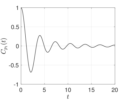
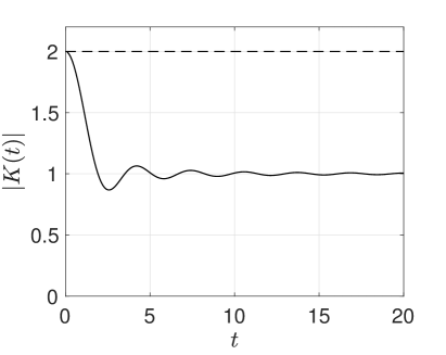
Figure 1: Harmonic chain of oscillators. (a) Velocity auto-correlation function $C_{p_{1}}(t)$ and (b) memory kernel $K(t)$ of the corresponding MZ equation. It is seen that our theoretical estimate (91) (dashed line) correctly bounds the MZ memory kernel. The upper bound we obtain is of the same order of magnitude as the memory kernel.

4.1.2 Hald System

In this section, we study the Hald Hamiltonian system studied by Chorin et. al. in [8, 11]. The Hamiltonian is given by

$$\mathcal{H}:=\frac{1}{2}(q_{1}^{2}+p_{1}^{2}+q_{2}^{2}+p_{2}^{2}+q_{1}^{2}q_{2}^{2}),$$ (92)

while the corresponding Hamilton’s equations of motion are

$$\begin{cases}\dot{q}_{1}&=p_{1}\\ \dot{p}_{1}&=-q_{1}(1+q_{2}^{2})\\ \dot{q}_{2}&=p_{2}\\ \dot{p}_{2}&=-q_{2}(1+q_{1}^{2})\end{cases}$$ (93)

We assume that the initial state is distributed according to canonical Gibbs distribution $\rho_{eq}=e^{-\beta\mathcal{H}}/Z$, where we set $\beta=1$ for simplicity. The partition function $Z$ is given by

$$Z=e^{1/4}(2\pi)^{3/2}K_{0}\left(\frac{1}{4}\right),$$ (94)

where $K_{0}(t)$ is the modified Bessel function of the second kind. We aim to study the properties of the autocorrelation function of the first component $q_{1}$, which is defined as

$$C_{q_{1}}(t)=\frac{\langle q_{1}(0),q_{1}(t)\rangle_{eq}}{\langle q_{1}(0),q_{1}(0)\rangle_{eq}}$$

Obviously, $C_{q_{1}}(0)=1$. The evolution equation for $C_{q_{1}}(t)$ is obtained by using the MZ formulation with the Mori’s projection

$$\mathcal{P}(\cdot)=\frac{\langle(\cdot),q_{1}(0)\rangle_{eq}}{\langle q_{1}(0),q_{1}(0)\rangle_{eq}}q_{1}(0)$$ (95)

This yields the GLE

$$\frac{dC_{q_{1}}(t)}{dt}=\Omega_{q_{1}}C_{q_{1}}(t)-\int_{0}^{t}K(s)C_{q_{1}}(t-s)ds.$$ (96)

The streaming term $\Omega_{q_{1}}C_{q_{1}}(t)$ is again identically zero, since

$$\Omega_{q_{1}}=\frac{\langle\mathcal{L}q_{1}(0),q_{1}(0)\rangle_{eq}}{\langle q_{1}(0),q_{1}(0)\rangle_{eq}}=0.$$

Theorem 3.8 provides the following computable upper bound for the modulus of $K(t)$

$$|K(t)|\leq\frac{\|\dot{q}_{1}(0)\|^{2}_{L^{2}_{\rho_{eq}}}}{\|q_{1}(0)\|^{2}_{L^{2}_{\rho_{eq}}}}=\frac{\|p_{1}(0)\|^{2}_{L^{2}_{\rho_{eq}}}}{\|q_{1}(0)\|^{2}_{L^{2}_{\rho_{eq}}}}=\frac{\displaystyle e^{1/4}K_{0}\left(1/4\right)}{\displaystyle\sqrt{\pi}U\left(1/2,0,1/2\right)}\approx 1.39786$$ (97)

where $U(a,b,y)$ is the confluent hypergeometric function of the second kind. In Figure 2, we plot the correlation function $C_{q_{1}}(t)$ that we obtain numerically with Markov Chain Monte Carlo, and the memory kernel $K(t)$

     (a)                                                              (b)

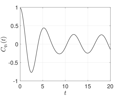
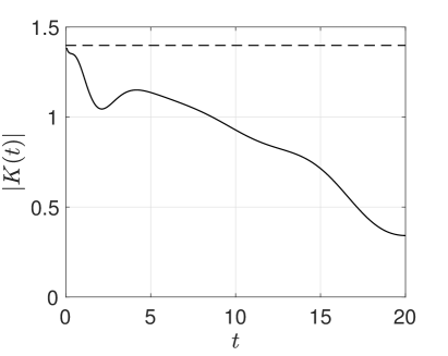
Figure 2: Hald Hamiltonian system (93). (a) Autocorrelation function of the displacement $q_{1}(t)$ and (b) memory kernel of the governing MZ equation. Here $C_{q_{1}}(t)$ is computed by Markov chain Monte-Carlo (MCMC) while $K(t)$ is determined by inverting numerically the Laplace transform in (98) with the Talbot algorithm. It is seen that the theoretical upper bound (97) (dashed line) is of the same order of magnitude as the memory kernel.

4.2 Non-Hamiltonian Systems with Infinite-Rank Projections

In this section we study the accuracy of the $t$-model, the $H$-model and the $H_{t}$ model in predicting scalar quantities of interest in non-Hamiltonian systems. In particular, we consider the MZ formulation with Chorin’s projection operator. For the particular case of linear dynamical systems we also compute the theoretical upper bounds we obtained in §3.5 for the memory growth and the error in the $H$-model, and compare such bounds with exact results.

4.2.1 Linear Dynamical Systems

We begin by considering a low-dimensional linear dynamical system $\dot{x}=Ax$ evolving from a random initial state with density $\rho_{0}(x)$ to verify the MZ memory estimates we obtained in §3.5. For simplicity, we choose $A$ to be negative definite

$$A=e^{C}Be^{-C},\qquad{B}=\begin{bmatrix}-\frac{1}{8}&0&0\\ 0&-\frac{2}{3}&0\\ 0&0&-\frac{1}{2}\end{bmatrix},\qquad{C}=\begin{bmatrix}0&1&0\\ -1&0&1\\ 0&-1&0\end{bmatrix}.$$ (99)

In this case, the origin of the phase space is a stable node and it is easy to estimate $\left\|e^{t\mathcal{L}}\right\|_{\rho_{0}}$ We set $x_{1}(0)=1$ and ${x_{2}(0),x_{3}(0)}$ independent standard normal random variables. In this setting, the semigroup estimates (69) and (70) are explicit

$$\|e^{t\mathcal{L}}\| \leq e^{t\omega},\quad\omega=-\frac{1}{2}\operatorname{Tr}(A)=0.6458,$$

$$\|e^{t\mathcal{L}\mathcal{Q}}\| \leq e^{t\omega_{\mathcal{Q}}},\quad\omega_{\mathcal{Q}}=\omega+\sqrt{A_{11}^{2}+\sum_{i=2}^{N}\frac{A_{1i}^{2}}{x_{1}^{2}(0)}}=1.1621.$$

Therefore, we obtain the following explicit upper bounds for the memory integral and the error of the $H$-model (see equations (71) and (73))

$$|w_{0}(t)| \leq 0.1964\left(e^{1.1621t}-e^{0.6458t}\right),$$ (100)

$$|w_{0}(t)-w_{0}^{n}(t)| \leq e^{1.1624t}\sqrt{\left(b^{T}\left(M_{11}^{T}\right)^{n}a_{1}\right)^{2}x_{1}^{2}(0)+\left\|\left(M_{11}^{T}\right)^{n+1}a\right\|_{2}^{2}}\frac{t^{n+1}}{(n+1)!}.$$ (101)

Next, we compare these error bounds with numerical results obtained by solving numerically the $H$-model (72). For example, the second-order $H$-model reads

$$\begin{dcases}\frac{d}{dt}\mathbb{E}[x_{1}(t)|x_{1}(0)]=-0.4560\mathbb{E}[x_{1}(t)|x_{1}(0)]+w_{0}^{2}(t),\\ \frac{dw_{0}^{2}(t)}{dt}=0.0586\mathbb{E}[x_{1}(t)|x_{1}(0)]+w_{1}^{2}(t),\\ \frac{dw_{1}^{2}(t)}{dt}=-0.0192\mathbb{E}[x_{1}(t)|x_{1}(0)].\end{dcases}$$ (102)

In Figure 3 we demonstrate convergence of the $H$-model to the benchmark solution computed by Monte-Carlo simulation as we increase the $H$-model differentiation order. In Figure 4 we plot the bound on the memory growth (equation (100)) and the bound in the memory error (equation (101)) together with exact results.

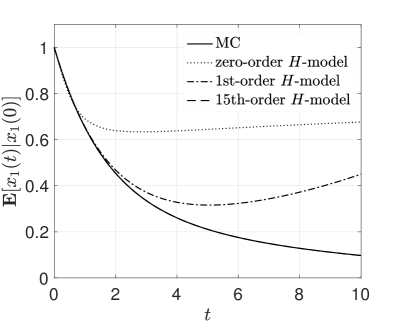
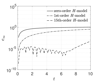
Figure 3: Convergence of the $H$-model for the linear dynamical system with matrix (99). The benchmark solution is computed with Monte-Carlo (MC) simulation. Also, the zero-order $H$-model represents the Markovian approximation to the MZ equation, i.e. the MZ equation without the memory term.

    (a)                                              (b)                                             (c)

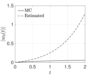
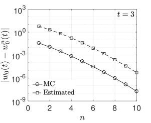
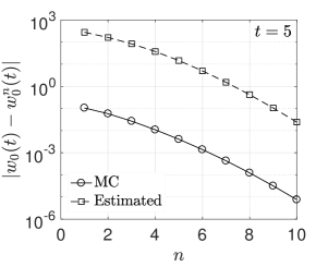
Figure 4: Linear dynamical system with matrix (99). In (a) we plot the memory term $w_{0}(t)$ we obtain from Monte Carlo simulation together with the estimated upper bound (100). In (b) and (c) we plot $H$-model approximation error $|w_{0}(T)-w_{0}^{n}(T)|$ together with the upper bound (101) for different differentiation orders $n$ and at different times $t$.

Remark

The results we just obtained can be obviously extended to higher-dimensional linear dynamical systems. In Figure 5 we plot the benchmark conditional mean path we obtained through Monte Carlo simulation together with the solution of the $H$-model (72) for the $100$-dimensional linear dynamical system defined by the matrix ($N=100$)

$$A=\begin{bmatrix}-1&1&&\dots&(-1)^{N}\\ 1&&&&\\ \vdots&&&B&\\ 1&&&&\end{bmatrix},$$ (103)

where $B=e^{C}\Lambda e^{-{C}}$ and

$${\Lambda}=\begin{bmatrix}-\frac{1}{8}&0&\cdots&0\\ 0&-\frac{2}{9}&&\vdots\\ \vdots&&\ddots&0\\ 0&\cdots&0&-\frac{N-1}{N+6}\end{bmatrix},\qquad{C}=\begin{bmatrix}0&1&&0\\ -1&0&\ddots&\\ &\ddots&\ddots&1\\ 0&&-1&0\end{bmatrix}.$$

It is seen that the $H$-model converges as we increase the differentiation order in any finite time interval, in agreement with the theoretical prediction of section 3.5.

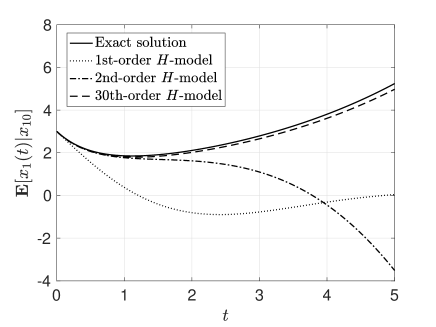
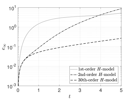
Figure 5: Linear dynamical system with matrix $A$ (103). Convergence of the $H$-model to the conditional mean path solution $\mathbb{E}[x_{1}(t)|x_{1}(0)]$. The initial condition is set as $x_{1}(0)=3$, while $\{x_{2}(0),\dots,x_{100}(0)\}$ are i.i.d. Normals.

4.2.2 Nonlinear Dynamical Systems

The hierarchical memory approximation method we discussed in section 3.4 can be applied to nonlinear dynamical systems in the form (1). As we will see, if we employ the $H_{t}$-model then the nonlinearity introduces a closure problem that needs to be addressed properly.

Lorenz-63 System

Consider the classical Lorenz-63 model

$$\begin{dcases}\dot{x}_{1}=\sigma(x_{2}-x_{1})\\ \dot{x}_{2}=x_{1}(r-x_{3})-x_{2}\\ \dot{x}_{3}=x_{1}x_{2}-\beta x_{3}\end{dcases}$$ (104)

where $\sigma=10$ and $\beta=8/3$. The phase space Liouville operator for this ODE is

$$\mathcal{L}=\sigma(x_{2}-x_{1})\frac{\partial}{\partial x_{1}}+(x_{1}(r-x_{3})-x_{2})\frac{\partial}{\partial x_{2}}+(x_{1}x_{2}-\beta x_{3})\frac{\partial}{\partial x_{3}}.$$

We choose the resolved variables to be $\hat{x}=\{x_{1},x_{2}\}$ and aim at formally integrating out $\tilde{x}={x_{3}}$ by using the Mori-Zwanzig formalism. To this end, we set $x_{3}(0)\sim\mathcal{N}(0,1)$ and consider the zeroth-order $H_{t}$-model ($t$-model)

$$\begin{dcases}\frac{dx_{1m}}{dt}=\sigma(x_{1m}-x_{2m}),\\ \frac{dx_{2m}}{dt}=-x_{2m}+rx_{1m}-tx_{1m}^{2}x_{2m},\end{dcases}$$ (105)

where $x_{1m}(t)=\mathbb{E}[x_{1}(t)|x_{1}(0),x_{2}(0)]$ and $x_{2m}(t)=\mathbb{E}[x_{2}(t)|x_{1}(0),x_{2}(0)]$ are conditional mean paths. To obtain this system we introduced the following mean field closure approximation

$$t\mathcal{P}e^{t\mathcal{L}}\mathcal{P}\mathcal{L}\mathcal{Q}\mathcal{L}x_{2}(0)= -t\mathbb{E}[x_{1}(t)^{2}x_{2}(t)|x_{1}(0),x_{2}(0)],$$

$$\simeq -t\mathbb{E}[x_{1}(t)|x_{1}(0),x_{2}(0)]^{2}\mathbb{E}[x_{2}(t)|x_{1}(0),x_{2}(0)],$$

$$= -tx_{1m}^{2}x_{2m}.$$ (106)

Higher-order $H_{t}$-models can be derived based on (106).

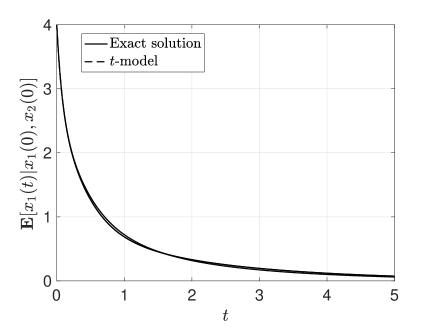
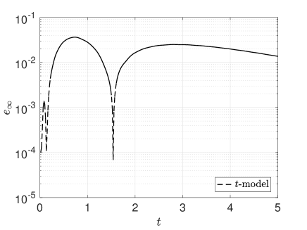
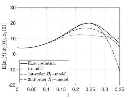
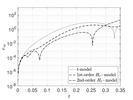
Figure 6: Accuracy of the $H_{t}$ model in representing the conditional mean path in the Lorenz-63 system (104). It is seen that if $r=0.5$ (first row), then the zeroth-order $H_{t}$-model, i.e., the $t$-model, is accurate for long integration times. On the other hand, if we consider the chaotic regime at $r=28$ (second row) then we see that the $t$-model and its high-order extension ($H_{t}$-model) are accurate only for relatively short time.

As is well known, if $r<1$, the fixed point $(0,0,0)$ is a global attractor and exponentially stable. In this case, the $t$-model (zeroth-order $H_{t}$-model) yields accurate prediction of the conditional mean path for long time (see Figure 6). On the other hand, if we consider the chaotic regime at $r=28$ then the $t$-model and its higher-order extension, i.e., the $H_{t}$-model, are accurate only for relatively short time. This is in agreement with our theoretical predictions. In fact, different from linear systems where the hierarchical representation of the memory integral can be proven to be convergent for long time, in nonlinear systems the memory hierarchy is, in general, provably convergent only in a short time period (Theorem 3.7 and Corollary 3.4.3). This doesn’t mean that the $H$-model or the $H_{t}$-model are not accurate for nonlinear systems. It just means that the accuracy depends on the system, the quantity of interest, and the initial condition.

Modified Lorenz-96 system.

As an example of a high dimensional nonlinear dynamical system, we consider the following modified Lorenz-96 system [21, 24]

$$\begin{dcases}\dot{x}_{1}=-x_{1}+x_{1}x_{2}+F\\ \dot{x}_{2}=-x_{2}+x_{1}x_{3}+F\\ \quad\vdots\\ \dot{x_{i}}=-x_{i}+(x_{i+1}-x_{i-2})x_{i-1}+F\\ \quad\vdots\\ \dot{x}_{N}=x_{N}-x_{N-2}x_{N-1}+F\end{dcases}$$ (107)

where $F$ is constant. As is well known, depending on the values of $N$ and $F$ this system can exhibit a wide range of behaviors [21]. Suppose we take the resolved variables to be $\hat{x}=\{x_{1},x_{2}\}$. Correspondingly, the unresolved ones, i.e., those we aim at integrating through the MZ framework, are $\tilde{x}=\{x_{3},\dots,x_{N}\}$, which we set to be independent standard normal random variables. By using the mean field approximation (106), we obtain the following zeroth-order $H_{t}$-model ($t$-model) of the modified Lorenz-96 system is (107)

$$\begin{dcases}\dot{x}_{1m}=-x_{1m}+x_{1m}x_{2m}+F,\\ \dot{x}_{2m}=-x_{2m}+F+t(x_{1m}^{2}x_{2m}-x_{1m}F).\\ \end{dcases}$$ (108)

In Figure 7 we study the accuracy of the $H_{t}$-model in representing the conditional mean path for with $F=5$ and $N=100$. It is seen that the the $H_{t}$-model converges only for short time (in agreement with the theoretical predictions) and it provides results that are more accurate that the classical $t$-model.

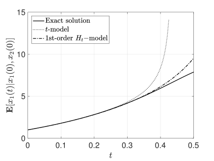
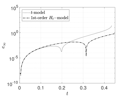
Figure 7: Accuracy of the $H_{t}$-model in representing the conditional mean path in the Lorenz-96 system (104). Here we set $F=5$ and $N=100$. It is seen that the $H_{t}$-model converges only for short time and provides results that are more accurate that the classical $t$-model.

5 Summary

In this paper we developed a thorough mathematical analysis to deduce conditions for accuracy of different approximations of the memory integral in the Mori-Zwanzig equation, and, more importantly, whether the algorithms to approximate such memory integral converge. In particular, we studied the short memory approximation, the $t$-model and various hierarchical memory approximation techniques. We also derived computable upper bounds for the MZ memory integral, which allowed us to estimate a priori the contribution of the memory to the dynamics. To the best of our knowledge, this is the first time rigorous convergence analysis is presented on approximations of the MZ memory integral. We found that for a given nonlinear dynamical system and quantity of interest, the approximation error can be controlled by setting constraints on the initial condition of the system, i.e., by preparing the system appropriately. We have also established rigorous convergence results for hierarchical memory approximation methods such as the $H$-model, the Type-I and Type II finite memory approximations, and the $H_{t}$ model. These methods converge for any finite integration time in the case of linear dynamical systems. However, for general nonlinear systems, the memory approximation problem remains challenging and convergence of the hierarchical methods we discussed in this paper can be granted only for short time, or on a case-by-case basis. We presented simple numerical examples demonstrating convergence of the $H$-model and $H_{t}$-model for prototype linear and nonlinear dynamical systems. The numerical results are found to be in agreement with the theoretical predictions.

Acknowledgements

This work was supported by the Air Force Office of Scientific Research Grant No. FA9550-16-586-1-0092.

Appendix A Semigroup Bounds via Function Decomposition

In looking for the numerical abscissa [13] (i.e., the logarithmic norm) of $\mathcal{L}\mathcal{Q}$, we seek to bound

$$\sup_{\mathcal{D}(\mathcal{L}\mathcal{Q})\ni x\neq 0}\Re\frac{\langle x,\mathcal{L}\mathcal{Q}x\rangle_{\sigma}}{\langle x,x\rangle_{\sigma}}.$$

Notice that, if $\mathcal{P}\mathcal{L}\mathcal{Q}=0$, then $\mathcal{L}\mathcal{Q}=\mathcal{Q}\mathcal{L}\mathcal{Q}$, so that we have the previously proven bound

$$\sup\Re\frac{\langle x,\mathcal{Q}\mathcal{L}\mathcal{Q}x\rangle_{\sigma}}{\langle x,x\rangle_{\sigma}}\leq-\frac{1}{2}\inf\operatorname{div}_{\sigma}\mathbf{F}.$$

In this section, we consider what happens when $\mathcal{P}\mathcal{L}\mathcal{Q}\neq 0$. To that end, let us note that $x\in\mathcal{D}(\mathcal{L}\mathcal{Q})$ may be decomposed as

$$x=\mathcal{Q}x+\alpha\mathcal{P}\mathcal{L}\mathcal{Q}x+\mathcal{P}y$$

where $\alpha\in\mathbb{C}$ and $\mathcal{P}y$ is orthogonal to $\mathcal{P}\mathcal{L}\mathcal{Q}x$. In other words, we define $\mathcal{P}y$ as

$$\mathcal{P}y:=\mathcal{P}x-\frac{\langle\mathcal{P}\mathcal{L}\mathcal{Q}x,\mathcal{P}x\rangle_{\sigma}}{\langle\mathcal{P}\mathcal{L}\mathcal{Q}x,\mathcal{P}\mathcal{L}\mathcal{Q}x\rangle_{\sigma}}\mathcal{P}\mathcal{L}\mathcal{Q}x,$$

and define $\alpha$ as

$$\alpha:=\frac{\langle\mathcal{P}\mathcal{L}\mathcal{Q}x,\mathcal{P}x\rangle_{\sigma}}{\langle\mathcal{P}\mathcal{L}\mathcal{Q}x,\mathcal{P}\mathcal{L}\mathcal{Q}x\rangle_{\sigma}}.$$

Then

$$\Re\frac{\langle x,\mathcal{L}\mathcal{Q}x\rangle_{\sigma}}{\langle x,x\rangle_{\sigma}} =\Re\frac{\langle\mathcal{Q}x+\alpha\mathcal{P}\mathcal{L}\mathcal{Q}x+\mathcal{P}y,\mathcal{L}\mathcal{Q}x\rangle_{\sigma}}{\langle x,x\rangle_{\sigma}},$$

$$=\frac{\Re\langle\mathcal{Q}x,\mathcal{L}\mathcal{Q}x\rangle_{\sigma}+\Re(\alpha)\|\mathcal{P}\mathcal{L}\mathcal{Q}x\|_{\sigma}^{2}}{\|\mathcal{Q}x\|_{\sigma}^{2}+|\alpha|^{2}\|\mathcal{P}\mathcal{L}\mathcal{Q}x\|_{\sigma}^{2}+\|\mathcal{P}y\|_{\sigma}^{2}},$$

$$\leq\max\left[0,\;\frac{\Re\langle\mathcal{Q}x,\mathcal{L}\mathcal{Q}x\rangle_{\sigma}+\Re(\alpha)\|\mathcal{P}\mathcal{L}\mathcal{Q}x\|_{\sigma}^{2}}{\|\mathcal{Q}x\|_{\sigma}^{2}+|\alpha|^{2}\|\mathcal{P}\mathcal{L}\mathcal{Q}x\|_{\sigma}^{2}}\right].$$

Since we assume $\mathcal{P}\mathcal{L}\mathcal{Q}\neq 0$, there exists $x$ such that $\mathcal{P}\mathcal{L}\mathcal{Q}x\neq 0$ and then, for any $\alpha$ such that

$$\Re(\alpha)\geq\frac{\Re\langle\mathcal{Q}x,\mathcal{L}\mathcal{Q}x\rangle_{\sigma}}{\|\mathcal{P}\mathcal{L}\mathcal{Q}x\|_{\sigma}^{2}},$$

we have

$$\Re\langle\mathcal{Q}x,\mathcal{L}\mathcal{Q}x\rangle_{\sigma}+\Re(\alpha)\|\mathcal{P}\mathcal{L}\mathcal{Q}x\|_{\sigma}^{2}\geq 0,$$

so that, for $\mathcal{P}\mathcal{L}\mathcal{Q}\neq 0$,

$$\sup_{\mathcal{D}(\mathcal{L}\mathcal{Q})\ni x\neq 0}\Re\frac{\langle x,\mathcal{L}\mathcal{Q}x\rangle_{\sigma}}{\langle x,x\rangle_{\sigma}}=\sup_{\mathcal{D}(\mathcal{L}\mathcal{Q})\ni x\neq 0}\frac{\Re\langle\mathcal{Q}x,\mathcal{L}\mathcal{Q}x\rangle_{\sigma}+\Re(\alpha)\|\mathcal{P}\mathcal{L}\mathcal{Q}x\|_{\sigma}^{2}}{\|\mathcal{Q}x\|_{\sigma}^{2}+|\alpha|^{2}\|\mathcal{P}\mathcal{L}\mathcal{Q}x\|_{\sigma}^{2}}.$$

Now, fix any $\mathcal{Q}x\in\mathcal{D}(\mathcal{L})\neq 0$ and consider the expression

$$\frac{\Re\langle\mathcal{Q}x,\mathcal{L}\mathcal{Q}x\rangle_{\sigma}+\Re(\alpha)\|\mathcal{P}\mathcal{L}\mathcal{Q}x\|_{\sigma}^{2}}{\|\mathcal{Q}x\|_{\sigma}^{2}+|\alpha|^{2}\|\mathcal{P}\mathcal{L}\mathcal{Q}x\|_{\sigma}^{2}}=\frac{\xi+\Re(\alpha)\beta^{2}}{1+|\alpha|^{2}\beta^{2}}$$

where

$$\xi=\xi(\mathcal{Q}x)=\Re\frac{\langle\mathcal{Q}x,\mathcal{L}\mathcal{Q}x\rangle_{\sigma}}{\|\mathcal{Q}x\|_{\sigma}^{2}},\qquad\beta=\beta(\mathcal{Q}x)=\frac{\|\mathcal{P}\mathcal{L}\mathcal{Q}x\|_{\sigma}}{\|\mathcal{Q}x\|_{\sigma}}.$$

Then, for this fixed $\mathcal{Q}x$,

$$\frac{\xi+\Re(\alpha)\beta^{2}}{1+|\alpha|^{2}\beta^{2}}\leq\max_{a\in\mathbb{R}}\frac{\xi+a\beta^{2}}{1+a^{2}\beta^{2}}.$$

Differentiating w.r.t. $a$ and setting equal to zero, we find that the latter expression is extremized when

$$0 =\beta^{2}(1+a^{2}\beta^{2})-2a\beta^{2}(\xi+a\beta^{2}),$$

i.e., when

$$\beta^{2}a^{2}+2\xi a-1 =0,\qquad a=\frac{-\xi\pm\sqrt{\xi^{2}+\beta^{2}}}{\beta^{2}}.$$

Since $\beta^{2}>0$, $\displaystyle\frac{\xi+a\beta^{2}}{1+a^{2}\beta^{2}}$ is maximized at $\displaystyle\hat{a}=\frac{-\xi+\sqrt{\xi^{2}+\beta^{2}}}{\beta^{2}}$. Then

$$\xi+\hat{a}\beta^{2}=\sqrt{\xi^{2}+\beta^{2}},\qquad 1+\hat{a}^{2}\beta^{2}=2\left(1-\xi\hat{a}\right)=2\left(\frac{\xi^{2}+\beta^{2}-\xi\sqrt{\xi^{2}+\beta^{2}}}{\beta^{2}}\right),$$

so that

$$\max_{a\in\mathbb{R}}\frac{\xi+a\beta^{2}}{1+a^{2}\beta^{2}}=\frac{\xi+\hat{a}\beta^{2}}{1+\hat{a}^{2}\beta^{2}}=\frac{1}{2}\frac{\beta^{2}}{\sqrt{\xi^{2}+\beta^{2}}-\xi}=\frac{1}{2}\left(\sqrt{\xi^{2}+\beta^{2}}+\xi\right).$$

Therefore,

$$\sup_{\mathcal{D}(\mathcal{L}\mathcal{Q})\ni x\neq 0}\Re\frac{\langle x,\mathcal{L}\mathcal{Q}x\rangle_{\sigma}}{\langle x,x\rangle_{\sigma}}=\sup_{\mathcal{D}(\mathcal{L})\ni(\mathcal{Q}x)\neq 0}\frac{1}{2}\left[\sqrt{\xi^{2}(\mathcal{Q}x)+\beta^{2}(\mathcal{Q}x)}+\xi(\mathcal{Q}x)\right].$$

When $\mathcal{P}\mathcal{L}\mathcal{Q}$ is unbounded, which is the typical case when $\mathcal{P}$ is an infinite-rank projection, such as most conditional expectations, there is unlikely to be a finite numerical abscissa for $\mathcal{L}\mathcal{Q}$. In particular, notice that if $\operatorname{div}_{\sigma}({F})$ is a bounded function (bounded both above and below), then $\xi(\mathcal{Q}x)$ is bounded for all $\mathcal{Q}x$ while $\beta(\mathcal{Q}x)$ is unbounded, in which case

$$\sup_{\mathcal{D}(\mathcal{L}\mathcal{Q})\ni x\neq 0}\Re\frac{\langle x,\mathcal{L}\mathcal{Q}x\rangle_{\sigma}}{\langle x,x\rangle_{\sigma}}=\infty.$$

It follows [35, 28] that in these cases, $\|e^{t\mathcal{L}\mathcal{Q}}\|_{\sigma}$ has infinite slope at $t=0$, and therefore there is no finite $\omega$ such that $\|e^{t\mathcal{L}\mathcal{Q}}\|_{\sigma}\leq e^{\omega t}$ for all $t\geq 0$ (see [13]). Assuming still that $\mathcal{L}\mathcal{Q}$ generates a strongly continuous semigroup, we must look to bound the semigroup as $\|e^{t\mathcal{L}\mathcal{Q}}\|_{\sigma}\leq Me^{\omega t}$, where

$$\omega>\omega_{0}=\lim_{t\to\infty}\frac{\ln\|e^{t\mathcal{L}\mathcal{Q}}\|_{\sigma}}{t}$$

and

$$M\geq M(\omega)=\sup\{\|e^{t\mathcal{L}\mathcal{Q}}\|_{\sigma}e^{-\omega t}:t\geq 0\}.$$

On the other hand, if $\mathcal{P}\mathcal{L}\mathcal{Q}$ is a bounded operator, for example when $\mathcal{P}$ is a finite-rank projection (e.g., Mori’s projection (12)), there exists a finite value for the numerical abscissa. Indeed, in this case, since $\zeta$ is bounded by $\omega=-\inf\operatorname{div}_{\sigma}({F})$, the numerical abscissa of $\mathcal{L}\mathcal{Q}$ may be bounded as

$$\omega_{\mathcal{L}\mathcal{Q}}:=\sup_{\mathcal{D}(\mathcal{L}\mathcal{Q})\ni x\neq 0}\Re\frac{\langle x,\mathcal{L}\mathcal{Q}x\rangle_{\sigma}}{\langle x,x\rangle_{\sigma}}\leq\frac{1}{2}\left[\sqrt{\omega^{2}+\|\mathcal{P}\mathcal{L}\mathcal{Q}\|_{\sigma}^{2}}+\omega\right].$$ (115)

Alternatively, in the case of finite rank $\mathcal{P}$, the operator $\mathcal{L}\mathcal{Q}$ may be thought of as a bounded perturbation of $\mathcal{L}$, i.e. $\mathcal{L}\mathcal{Q}=\mathcal{L}-\mathcal{L}\mathcal{Q}$, and the numerical abscissa of $\mathcal{L}\mathcal{Q}$ can be bounded using the bounded perturbation theorem [15, III.1.3], obtaining

$$\omega_{\mathcal{L}\mathcal{Q}}\leq\omega+\|\mathcal{L}\mathcal{P}\|_{\sigma}.$$ (116)

Either of these bounds for $\omega_{\mathcal{L}\mathcal{Q}}$ can be used to bound the semigroup norm

$$\|e^{t\mathcal{L}\mathcal{Q}}\|_{\sigma} \leq e^{\omega_{\mathcal{L}\mathcal{Q}}t}\leq e^{\frac{1}{2}\left(\sqrt{\omega^{2}+\|\mathcal{P}\mathcal{L}\mathcal{Q}\|_{\sigma}^{2}}+\omega\right)t}$$

$$\|e^{t\mathcal{L}\mathcal{Q}}\|_{\sigma} \leq e^{\omega_{\mathcal{L}\mathcal{Q}}t}\leq e^{(\omega+\|\mathcal{L}\mathcal{P}\|_{\sigma})t}.$$

Which of these two estimates gives the tighter bound will generally depend on the values of $\|\mathcal{P}\mathcal{L}\mathcal{Q}\|_{\sigma}$ and $\|\mathcal{L}\mathcal{P}\|_{\sigma}$. It may be noted, however, that, when $\sigma$ is invariant, $\omega=0$ and $\mathcal{L}$ is skew-adjoint, so that

$$\|\mathcal{P}\mathcal{L}\mathcal{Q}\|_{\sigma}=\|\mathcal{Q}\mathcal{L}^{{\dagger}}\mathcal{P}\|_{\sigma}=\|\mathcal{Q}\mathcal{L}\mathcal{P}\|_{\sigma}\leq\|\mathcal{L}\mathcal{P}\|_{\sigma}$$

and therefore the bound in (115) is half that of (116).

Appendix B The Mori-Zwanzig Formulation in PDF Space

It was shown in [14] that the Banach dual of (4) defines an evolution in the probability density function space. Specifically, the joint probability density function of the state vector $u(t)$ that solves equation (1) is pushed forward by the Frobenius-Perron operator $\mathcal{F}(t,0)$ (Banach dual of the Koopman operator (3))

$$p(x,t)=\mathcal{F}(t,s)p(x,s),\qquad\mathcal{F}(t,s)=e^{(t-s)\mathcal{M}},$$ (118)

where

$$\mathcal{M}(x)p(x,t)=-\nabla\cdot(F(x)p(x,t)).$$ (119)

By introducing a projection $\mathcal{P}$ in the space of probability density functions and its complement $\mathcal{Q}=\mathcal{I}-\mathcal{P}$, it is easy to show that the projected density $\mathcal{P}p$ satisfies the MZ equation [40]

$$\frac{\partial\mathcal{P}p(t)}{\partial t}=\mathcal{PMP}p(t)+\mathcal{P}e^{t\mathcal{QM}}\mathcal{Q}p(0)+\int_{0}^{t}\mathcal{PM}e^{(t-s)\mathcal{QM}}\mathcal{QMP}p(s)ds.$$ (120)

In the next sections we perform an analysis of different types of approximations of the MZ memory integral

$$\int_{0}^{t}\mathcal{PM}e^{(t-s)\mathcal{QM}}\mathcal{QMP}p(s)ds.$$ (121)

The main objective of such analysis is to establish rigorous error bounds for widely used approximation methods, and also propose new provably convergent approximation schemes.

B.1 Analysis of the Memory Integral

In this section, we develop the analysis of the memory integral arising in the PDF formulation of the MZ equation. The starting point is the definition (121). As before, we begin with the following estimate of upper bound estimation of the integral

Theorem B.1.

(Memory growth) Let $e^{t\mathcal{MQ}}$ and $e^{t\mathcal{M}}$ be strongly continuous semigroups with upper bounds $\|e^{t\mathcal{M}}\|\leq Me^{t\omega}$ and $\|e^{t\mathcal{M}\mathcal{Q}}\|\leq M_{{\mathcal{Q}}}e^{t\omega_{\mathcal{Q}}}$, and let $T>0$ be a fixed integration time. Then for any $0\leq t\leq T$ we have

$$\bigg{\|}\int_{0}^{t}\mathcal{PM}e^{(t-s)\mathcal{Q\mathcal{M}}}\mathcal{Q\mathcal{M}P}p(s)ds\bigg{\|}\leq N_{0}(t),$$

where

$$N_{0}(t)=\begin{dcases}tC_{4},\quad&\omega_{\mathcal{Q}}=0;\\ \frac{C_{4}}{\omega_{\mathcal{Q}}}(e^{t\omega_{\mathcal{Q}}}-1),\quad&\omega_{\mathcal{Q}}\neq 0;\end{dcases}$$

and $\displaystyle C_{4}=\max_{0\leq s\leq T}\|\mathcal{P}\|\|\mathcal{M}\mathcal{P}\mathcal{M}p(s)\|$. Moreover, $N(t)$ satisfies $\displaystyle\lim_{t\rightarrow 0}N(t)=0$.

Proof.

Consider

$$\bigg{\|}\int_{0}^{t}\mathcal{PM}e^{(t-s)\mathcal{Q\mathcal{M}}}\mathcal{Q\mathcal{M}P}p(s)ds\bigg{\|} =\bigg{\|}\int_{0}^{t}\mathcal{P}e^{(t-s)\mathcal{M}\mathcal{Q}}\mathcal{M}\mathcal{Q\mathcal{M}P}p(s)ds\bigg{\|}$$

$$\leq C_{4}M_{\mathcal{Q}}\int_{0}^{t}e^{(t-s)\omega_{\mathcal{Q}}}ds$$

$$=\begin{dcases}tC_{4},\quad&\omega_{\mathcal{Q}}=0\\ \frac{C_{4}}{\omega_{\mathcal{Q}}}(e^{t\omega_{\mathcal{Q}}}-1),\quad&\omega_{\mathcal{Q}}\neq 0\end{dcases}$$

where $\displaystyle C_{4}=\max_{0\leq s\leq T}\|\mathcal{P}\|\|\mathcal{M}\mathcal{Q}\mathcal{M}\mathcal{P}p(s)\|$.

$\Box$

Theorem B.2.

(Memory approximation via the $t$-model) Let $e^{t\mathcal{MQ}}$ and $e^{t\mathcal{M}}$ be strongly continuous semigroups with bounds $\|e^{t\mathcal{M}}\|\leq Me^{t\omega}$ and $\|e^{t\mathcal{M}\mathcal{Q}}\|\leq M_{{\mathcal{Q}}}e^{t\omega_{\mathcal{Q}}}$, and let $T>0$ be a fixed integration time. If the function $k(s,t)=\mathcal{P\mathcal{M}}e^{(t-s)\mathcal{Q\mathcal{M}}}\mathcal{Q\mathcal{M}P}p(s)$ (integrand of the memory term) is at least twice differentiable respect to $s$ for all $t\geq 0$, then

$$\bigg{\|}\int_{0}^{t}\mathcal{P\mathcal{M}}e^{(t-s)\mathcal{Q\mathcal{M}}}\mathcal{Q\mathcal{M}P}p(s)ds-t\mathcal{P\mathcal{M}Q\mathcal{M}P}p(t)\bigg{\|}\leq N_{1}(t)$$

where $N_{1}(t)$ is defined as

$$N_{1}(t)=\begin{dcases}t(M_{\mathcal{Q}}+1)C_{4},\quad&\omega_{\mathcal{Q}}=0\\ \frac{C_{2}M_{\mathcal{Q}}}{\omega_{\mathcal{Q}}}(e^{t\omega_{\mathcal{Q}}}-1)+tC_{4},\quad&\omega_{\mathcal{Q}}\neq 0\end{dcases}$$

and $C_{4}$ is as in Theorem B.1.

Proof.

$$\bigg{\|}\int_{0}^{t}\mathcal{PM}e^{(t-s)\mathcal{QM}}\mathcal{QMP}p(s)ds-t\mathcal{PMQMP}p(t)\bigg{\|} \leq C_{4}M_{\mathcal{Q}}\int_{0}^{t}e^{(t-s)\omega_{\mathcal{Q}}}ds+C_{4}t$$

$$=\begin{dcases}t(M_{\mathcal{Q}}+1)C_{4},\quad&\omega_{\mathcal{Q}}=0\\ \frac{C_{4}M_{\mathcal{Q}}}{\omega_{\mathcal{Q}}}(e^{t\omega_{\mathcal{Q}}}-1)+tC_{4},\quad&\omega_{\mathcal{Q}}\neq 0\end{dcases}$$

$\Box$

B.2 Hierarchical Memory Approximation in PDF Space

The hierarchical memory approximation methods we discussed in section 3.4 can be also developed in the PDF space. To this end, let us first define

$$v_{0}(t)=\int_{0}^{t}\mathcal{P\mathcal{M}}e^{(t-s)\mathcal{Q\mathcal{M}}}\mathcal{Q\mathcal{M}P}p(s)ds.$$ (122)

By repeatedly differentiating $v_{0}(t)$ with respect to time (assuming $v_{0}(t)$ smooth enough) we obtain the hierarchy of equations

$$\frac{\partial}{\partial t}v_{i-1}(t)=\mathcal{P\mathcal{M}}(\mathcal{Q\mathcal{M}})^{i}\mathcal{P}p(t)+v_{i}(t)\qquad i=1,\dots,n$$

where,

$$v_{i}(t)=\int_{0}^{t}\mathcal{P\mathcal{M}}e^{(t-s)\mathcal{Q\mathcal{M}}}(\mathcal{Q\mathcal{M}})^{i+1}\mathcal{P}p(s)ds.$$

By following closely the discussion in section 3.4 we introduce the hierarchy of memory equations

$$\begin{cases}\displaystyle\frac{dv_{0}^{n}(t)}{dt}=\mathcal{P\mathcal{M}}\mathcal{Q\mathcal{M}}\mathcal{P}p(t)+v_{1}^{n}(t)\vspace{0.2cm}\\ \displaystyle\frac{dv_{1}^{n}(t)}{dt}=\mathcal{P\mathcal{M}}(\mathcal{Q\mathcal{M}})^{2}\mathcal{P}p(t)+v_{2}^{n}(t)\\ \hskip 14.22636pt\vdots\\ \displaystyle\frac{dv_{n-1}^{n}(t)}{dt}=\mathcal{P\mathcal{M}}(\mathcal{Q\mathcal{M}})^{n}\mathcal{P}p(t)+v_{n}^{e_{n}}(t)\end{cases}$$ (123)

and approximate the last term in such hierarchy in different ways. Specifically, we consider

$$v_{n}^{e_{n}}(t) =\int_{t}^{t}\mathcal{P\mathcal{M}}e^{(t-s)\mathcal{Q\mathcal{M}}}(\mathcal{Q\mathcal{M}})^{n+1}\mathcal{P}p(s)ds=0 \qquad(\text{$H$-model}),$$

$$v_{n}^{e_{n}}(t) =\int_{\max(0,t-\Delta t)}^{t}\mathcal{P\mathcal{M}}e^{(t-s)\mathcal{Q\mathcal{M}}}(\mathcal{Q\mathcal{M}})^{n+1}\mathcal{P}p(s)ds \qquad(\text{Type \@slowromancap i@ Finite Memory Approximation}),$$

$$v_{n}^{e_{n}}(t) =\int_{\min(t,t_{n})}^{t}\mathcal{P\mathcal{M}}e^{(t-s)\mathcal{Q\mathcal{M}}}(\mathcal{Q\mathcal{M}})^{n+1}\mathcal{P}p(s)ds \qquad(\text{Type \@slowromancap ii@ Finite Memory Approximation}),$$

$$v_{n}^{en}(t) =t\mathcal{P}\mathcal{M}(\mathcal{Q}\mathcal{M})^{n+1}\mathcal{P}p(t) \qquad(\text{$H_{t}$-model}).$$

Hereafter we establish the accuracy of the approximation schemes resulting from the substitution of each $v_{n}^{e_{n}}(t)$ above into (123).

Theorem B.3.

(Accuracy of the $H$-model) Let $e^{t\mathcal{M}}$ and $e^{t\mathcal{M}\mathcal{Q}}$ be strongly continuous semigroups, $T>0$ a fixed integration time, and

$$\beta_{i}=\frac{\displaystyle\sup_{s\in[0,T]}\|(\mathcal{M}\mathcal{Q})^{i+1}\mathcal{M}\mathcal{P}p(s)\|}{\displaystyle\sup_{s\in[0,T]}\|(\mathcal{M}\mathcal{Q})^{i}\mathcal{M}\mathcal{P}p(s)\|},\qquad 1\leq i\leq n.$$ (124)

Then for $1\leq q\leq n$ we have

$$\|v_{0}(t)-v_{0}^{q}(t)\|\leq N_{2}^{q}(t),$$

where

$$N_{2}^{q}(t)=A_{2}C_{4}\left(\prod_{i=1}^{q}\beta_{i}\right)\frac{t^{q+1}}{(q+1)!},$$

$\displaystyle A_{2}=\max_{s\in[0,T]}e^{s\omega_{\mathcal{Q}}}$, and $C_{4}$ is as in Theorem B.1.

Proof.

The error at the $n$-th level can be bounded as

$$\|v_{0}(t)-v_{0}^{q}(t)\| \leq\int_{0}^{t}\int_{0}^{\tau_{q}}\dots\int_{0}^{\tau_{2}}\|\mathcal{P}\mathcal{M}e^{(\tau_{1}-s)\mathcal{Q}\mathcal{M}}(\mathcal{Q}\mathcal{M})^{p+1}\mathcal{P}p(s)\|dsd\tau_{1}\dots d\tau_{q}$$

$$\leq A_{2}C_{4}\left(\prod_{i=1}^{q}\beta_{i}\right)\frac{t^{q+1}}{(q+1)!},$$

where

$$A_{2} =\max_{s\in[0,T]}e^{s\omega_{\mathcal{Q}}}=\begin{cases}1&\omega_{\mathcal{Q}}\leq 0\\ e^{T\omega_{\mathcal{Q}}}&\omega_{\mathcal{Q}}\geq 0\end{cases}.$$ (125)

Let

$$\beta_{i} =\frac{\displaystyle\sup_{s\in[0,T]}\|(\mathcal{M}\mathcal{Q})^{i+1}\mathcal{M}\mathcal{P}p(s)\|}{\displaystyle\sup_{s\in[0,T]}\|(\mathcal{M}\mathcal{Q})^{i}\mathcal{M}\mathcal{P}p(s)\|},$$ (126)

under the assumption that these quantities are finite. Then we have

$$\|v_{0}(t)-v_{0}^{q}(t)\|\leq A_{2}C_{4}\left(\prod_{i=1}^{q}\beta_{i}\right)\frac{t^{q+1}}{(q+1)!}.$$

$\Box$

Corollary B.3.1.

(Uniform convergence of the $H$-model) If $\beta_{i}$ in Theorem B.3 satisfy

$$\beta_{i}<\frac{i+1}{T},\quad 1\leq i\leq n$$

for any fixed time $T$, then there exits a sequence $\delta_{1}>\delta_{2}>\dots>\delta_{n}$ such that

$$\|v_{0}(T)-v_{0}^{q}(T)\|\leq\delta_{q},$$

where $1\leq q\leq n$.

Corollary B.3.2.

(Asymptotic convergence of the $H$-model) If $\beta_{i}$ in Theorem B.3 satisfy

$$\beta_{i}<C,\quad 1\leq i<+\infty$$

for some constant $C$, then for any fixed time $T$ and arbitrary $\delta>0$, there exits an integer $q$ such that for all $n>q$,

$$\|v_{0}(T)-v_{0}^{n}(T)\|\leq\delta.$$

The proofs of the Corollary B.3.1 and B.3.2 closely follow the proofs of Corollary 3.4.1 and 3.4.2. Therefore we omit details here.

Theorem B.4.

(Accuracy of Type-I FMA) Let $e^{t\mathcal{M}}$ and $e^{t\mathcal{M}\mathcal{Q}}$ be strongly continuous semigroups, $T>0$ a fixed integration time, and let

$$\beta_{i}=\frac{\displaystyle\sup_{s\in[0,T]}\|(\mathcal{M}\mathcal{Q})^{i+1}\mathcal{M}\mathcal{P}p(s)\|}{\displaystyle\sup_{s\in[0,T]}\|(\mathcal{M}\mathcal{Q})^{i}\mathcal{M}\mathcal{P}p(s)\|},\qquad 1\leq i\leq n.$$ (127)

Then for $1\leq q\leq n$

$$\|v_{0}(t)-v_{0}^{q}(t)\|\leq N_{3}^{q}(t),$$

where

$$N_{3}^{q}(t)=A_{2}C_{4}\left(\prod_{i=1}^{q}\beta_{i}\right)\frac{(t-\Delta t_{q})^{q+1}}{(q+1)!},$$

and $C_{4}$ is as in Theorem B.1.

Proof.

The proof is very similar with the proof of Theorem 3.5. We begin with the estimate of $v_{0}(t)-v_{0}^{q}(t)$

$$\int_{0}^{\max(0,t-\Delta t_{q})}\int_{0}^{\tilde{\tau}_{q}}\cdots\int_{0}^{\tilde{\tau}_{2}}\int_{0}^{\tilde{\tau}_{1}}\mathcal{P}e^{(\tilde{\tau}_{1}+\Delta t_{q}-s)\mathcal{M}\mathcal{Q}}(\mathcal{M}\mathcal{Q})^{q+1}\mathcal{M}\mathcal{Q}p(s)dsd\tilde{\tau}_{1}\cdots d\tilde{\tau}_{q},$$

$$=\begin{dcases}0&0\leq t\leq\Delta t_{q}\\ \int_{0}^{t-\Delta t_{q}}\int_{0}^{\sigma}\frac{(t-\Delta t_{q}-\sigma)^{q-1}}{(q-1)!}\mathcal{P}e^{(\sigma+\Delta t_{q}-s)\mathcal{M}\mathcal{Q}}(\mathcal{M}\mathcal{Q})^{q+1}\mathcal{M}\mathcal{Q}p(s)dsd\sigma&t\geq\Delta t_{q}.\end{dcases}$$

This can be bounded by following the technique in the proof of Theorem B.3. This yields

$$\|v_{0}(t)-v_{0}^{q}(t)\| \leq\begin{dcases}0&0\leq t\leq\Delta t_{q}\\ A_{2}C_{4}\left(\prod_{i=1}^{q}\beta_{i}\right)\frac{(t-\Delta t_{q})^{q+1}}{(q+1)!}&t\geq\Delta t_{q}\end{dcases}.$$ (129a)

$\Box$

Corollary B.4.1.

(Uniform convergence of Type-I FMA) If $\beta_{i}$ in Theorem B.4 satisfy

$$\beta_{i}<(i+1)\left[\frac{\delta i!}{C_{4}A_{2}\left(\prod_{k=1}^{i}\beta_{k}\right)}\right]^{-\frac{1}{i}}$$ (130)

then for any $\delta>0$, there exists an ordered time sequence $\Delta t_{n}<\Delta t_{n-1}<\dots<\Delta t_{1}<T$ such that

$$\|w_{0}(T)-w_{0}^{q}(T)\|\leq\delta,\quad 1\leq q\leq n$$

and which satisfies

$$\Delta t_{q}\leq T-\left[\frac{\delta(q+1)!}{C_{4}A_{2}\left(\prod_{i=1}^{q}\beta_{i}\right)}\right]^{\frac{1}{q+1}}.$$

The proof is very similar with the proof of Corollary 3.5.1 and therefore we omit it.

Theorem B.5.

(Accuracy of Type-II FMA) Let $e^{t\mathcal{\mathcal{M}}}$ and $e^{t\mathcal{\mathcal{M}Q}}$ be strongly continuous semigroups and $T>0$ a fixed integration time. Set

$$\beta_{i}=\frac{\displaystyle\sup_{s\in[0,T]}\|(\mathcal{M}\mathcal{Q})^{i+1}\mathcal{M}\mathcal{P}p(s)\|}{\displaystyle\sup_{s\in[0,T]}\|(\mathcal{M}\mathcal{Q})^{i}\mathcal{M}\mathcal{P}p(s)\|},\qquad 1\leq i\leq n.$$ (131)

Then for $1\leq q\leq n$

$$\|v_{0}(t)-v_{0}^{q}(t)\|\leq N_{4}^{q}(t),$$

where

$$N_{4}^{q}(t)=\frac{C_{4}}{\omega_{\mathcal{Q}}}\big{[}1-e^{-t_{q}\omega_{\mathcal{Q}}}\big{]}\left(\prod_{i=1}^{q}\beta_{i}\right)f_{q}(\omega_{\mathcal{Q}},t),$$

$f_{q}(\omega_{\mathcal{Q}},t)$ is defined in (52) and $C_{4}$ is as in Theorem B.1.

Proof.

The proof is very similar with the proof of Theorem 3.6. Hereafter we provide the proof for the case when $\omega_{\mathcal{Q}}>0$. Other cases can be easily obtained by using the same method. First of all, we have error estimation

$$\|v_{0}(t)-v_{0}^{q}(t)\| \leq\int_{0}^{t}\int_{0}^{\tau_{q}}\cdots\int_{0}^{\tau_{2}}\int_{0}^{t_{q}}\|\mathcal{P}\mathcal{M}e^{(\tau_{1}-s)\mathcal{Q}\mathcal{M}}(\mathcal{Q}\mathcal{M})^{q+1}\mathcal{P}p(s)\|dsd\tau_{1}\cdots d\tau_{q}$$

$$\leq C_{4}\left(\prod_{i=1}^{q}\beta_{i}\right)\int_{0}^{t}\int_{0}^{\tau_{q}}\cdots\int_{0}^{\tau_{2}}\int_{0}^{t_{q}}e^{(\tau_{1}-s)\omega_{\mathcal{Q}}}dsd\tau_{1}\cdots d\tau_{q}$$

$$=\frac{C_{4}}{\omega_{\mathcal{Q}}}\big{[}1-e^{-t_{q}\omega_{\mathcal{Q}}}\big{]}\left(\prod_{i=1}^{q}\beta_{i}\right)f_{q}(\omega_{\mathcal{Q}},t),$$

where $f_{q}(\omega_{\mathcal{Q}},t)$ is as in (52).

$\Box$

Corollary B.5.1.

(Uniform convergence of Type-II FMA) If $\beta_{i}$ in Theorem B.5 satisfy

$$\begin{dcases}\beta_{i}<\frac{i}{T},\quad&\omega_{\mathcal{Q}}=0\\ \beta_{i}<\omega_{\mathcal{Q}}\frac{\displaystyle e^{T\omega_{\mathcal{Q}}}-\sum_{k=0}^{i-2}\frac{(T\omega_{\mathcal{Q}})^{k}}{k!}}{\displaystyle e^{T\omega_{\mathcal{Q}}}-\sum_{k=0}^{i-1}\frac{(T\omega_{\mathcal{Q}})^{k}}{k!}},\quad&\omega_{\mathcal{Q}}\neq 0\end{dcases}$$

for all $t\in[0,T]$, then for arbitrarily small $\delta>0$ there exists an ordered time sequence $0<t_{0}<t_{1}<\dots t_{n}<T$ such that

$$\|v_{0}(T)-v_{0}^{q}(T)\|\leq\delta,\quad 1\leq q\leq n$$

which satisfies

$$t_{q} \geq\frac{1}{\omega_{\mathcal{Q}}}\ln\left[1-\frac{\delta\omega_{\mathcal{Q}}^{q+1}}{\displaystyle C_{4}\left(\prod_{i=1}^{q}\beta_{i}\right)\left[e^{T\omega_{\mathcal{Q}}}-\sum_{k=0}^{q-1}\frac{(T\omega_{\mathcal{Q}})^{k}}{k!}\right]}\right].$$

Proof.

To ensure that $\|v_{0}(t)-v_{0}^{q}(t)\|\leq\delta$ for all $0\leq t\leq T$, we can take (for $\omega_{\mathcal{Q}}>0$)

$$\frac{C_{4}}{\omega_{\mathcal{Q}}}\big{[}1-e^{-t_{q}\omega_{\mathcal{Q}}}\big{]}\left(\prod_{i=1}^{q}\beta_{i}\right)f_{q}(\omega_{\mathcal{Q}},T)=\max_{t\in[0,T]}\frac{C_{2}}{\omega_{\mathcal{Q}}}\big{[}1-e^{-t_{q}\omega_{\mathcal{Q}}}\big{]}\left(\prod_{i=1}^{q}\beta_{i}\right)f_{q}(\omega_{\mathcal{Q}},t)\leq\delta.$$

Therefore

$$e^{-t_{q}\omega_{\mathcal{Q}}} \geq 1-\frac{\delta\omega_{\mathcal{Q}}}{\displaystyle C_{4}\left(\prod_{i=1}^{q}\beta_{i}\right)f_{q}(\omega_{\mathcal{Q}},T)}\qquad\textrm{i.e., }$$

$$t_{q} \leq\frac{1}{\omega_{\mathcal{Q}}}\ln\left[1-\frac{\delta\omega_{\mathcal{Q}}^{q+1}}{\displaystyle C_{4}\left(\prod_{i=1}^{q}\beta_{i}\right)\left[e^{T\omega_{\mathcal{Q}}}-\sum_{k=0}^{q-1}\frac{(T\omega_{\mathcal{Q}})^{k}}{k!}\right]}\right].$$

Since for $\omega_{\mathcal{Q}}>0$, we have have condition

$$\beta_{i}(t)<\omega_{\mathcal{Q}}\frac{\displaystyle e^{T\omega_{\mathcal{Q}}}-\sum_{k=0}^{i-2}\frac{(T\omega_{\mathcal{Q}})^{k}}{k!}}{\displaystyle e^{T\omega_{\mathcal{Q}}}-\sum_{k=0}^{i-1}\frac{(T\omega_{\mathcal{Q}})^{k}}{k!}}.$$

Thus, there exists an ordered time sequence $0<t_{1}<\dots<t_{n}$ such that $\|v_{0}(T)-v_{0}^{n}(T)\|\leq\delta$. As in Theorem 3.6, this $\delta$-bound on the error holds for all $t_{n}$ (with upper bound as above), which implies the existence of such an increasing time sequence $0<t_{1}<\dots<t_{n}$ with $t_{n}$ bounded from below by the same quantities.

$\Box$

References

- [1] J. Abate and W. Whitt. A unified framework for numerically inverting Laplace transforms. INFORMS Journal of Computing, 18(4):408–421, 2006.
- [2] B. J. Alder and T. E. Wainwright. Decay of the velocity autocorrelation function. Phys. Rev. A, 1(1):18, 1970.
- [3] R. J. Baxter. Exactly solved models in statistical mechanics. Elsevier, 2016.
- [4] N. Biggs. Algebraic graph theory. Cambridge University Press, 1993.
- [5] H.-P. Breuer, B. Kappler, and F. Petruccione. The time-convolutionless projection operator technique in the quantum theory of dissipation and decoherence. Ann. Physics, 291(1):36 – 70, 2001.
- [6] A. Chertock, D. Gottlieb, and A. Solomonoff. Modified optimal prediction and its application to a particle-method problem. J. Sci. Comput., 37(2):189–201, 2008.
- [7] H. Cho, D. Venturi, and G. E. Karniadakis. Statistical analysis and simulation of random shocks in Burgers equation. Proc. R. Soc. A, 2171(470):1–21, 2014.
- [8] A. Chorin, O. Hald, and R. Kupferman. Optimal prediction with memory. Physica D: Nonlinear Phenomena, 166(3-4):239–257, 2002.
- [9] A. J. Chorin, O. H. Hald, and R. Kupferman. Optimal prediction and the Mori-Zwanzig representation of irreversible processes. Proc. Natl. Acad. Sci. USA, 97(7):2968–2973, 2000.
- [10] A. J. Chorin, R. Kupferman, and D. Levy. Optimal prediction for Hamiltonian partial differential equations. J. Comput. Phys., 162(1):267–297, 2000.
- [11] A. J. Chorin and P. Stinis. Problem reduction, renormalization and memory. Comm. App. Math. and Comp. Sci., 1(1):1–27, 2006.
- [12] E. Darve, J. Solomon, and A. Kia. Computing generalized Langevin equations and generalized Fokker-Planck equations. Proc. Natl. Acad. Sci. USA, 106(27):10884–10889, 2009.
- [13] E. B. Davies. Semigroup growth bounds. J. Operator Theory, 53(2):225–249, 2005.
- [14] J. Dominy and D. Venturi. Duality and conditional expectations in the Nakajima-Mori-Zwanzig formulation. J. Math. Phys., 58:082701, 2017.
- [15] K.-J. Engel and R. Nagel. One-parameter semigroups for linear evolution equations, volume 194. Springer, 1999.
- [16] P. Español. Dissipative particle dynamics for a harmonic chain: A first-principles derivation. Phys. Rev. E, 53(2):1572, 1996.
- [17] J. Florencio, , and H. M. Lee. Exact time evolution of a classical harmonic-oscillator chain. Phys. Rev. A, 31(5):3231, 1985.
- [18] R. F. Fox. Functional-calculus approach to stochastic differential equations. Phys. Rev. A, 33(1):467–476, 1986.
- [19] S. Gudder. A Radon-Nikodým theorem for -algebras. Pacific J. Math., 80(1):141–149, 1979.
- [20] G. D. Harp and B. J. Berne. Time-correlation functions, memory functions, and molecular dynamics. Phys. Rev. A, 2(3):975, 1970.
- [21] A. Karimi and M. R. Paul. Extensive chaos in the Lorenz-96 model. Chaos, 20(4):043105(1–11), 2010.
- [22] J. Kim and I. Sawada. Dynamics of a harmonic oscillator on the Bethe lattice. Phys. Rev. E, 61(3):R2172, 2000.
- [23] B. O. Koopman. Hamiltonian systems and transformation in Hilbert spaces. Proc. Natl. Acad. Sci. USA, 17(5):315–318, 1931.
- [24] E. N. Lorenz. Predictability - A problem partly solved. In ECMWF seminar on predictability: Volume 1, pages 1–18, 1996.
- [25] H. Mori. A continued-fraction representation of the time-correlation functions. Progress of Theoretical Physics, 34(3):399–416, 1965.
- [26] H. Mori. Transport, collective motion, and Brownian motion. Prog. Theor. Phys., 33(3):423–455, 1965.
- [27] F. Moss and P. V. E. McClintock, editors. Noise in nonlinear dynamical systems. Volume 1: theory of continuous Fokker-Planck systems. Cambridge Univ. Press, 1995.
- [28] A. Pazy. Semigroups of linear operators and applications to partial differential equations. Springer, 1992.
- [29] I. Snook. The Langevin and generalised Langevin approach to the dynamics of atomic, polymeric and colloidal systems. Elsevier, first edition, 2007.
- [30] G. Söderlind. The logarithmic norm. History and modern theory. BIT Numerical Mathematics, 46(3):631–652, 2006.
- [31] P. Stinis. Stochastic optimal prediction for the Kuramoto–Sivashinsky equation. Multiscale Modeling & Simulation, 2(4):580–612, 2004.
- [32] P. Stinis. A comparative study of two stochastic model reduction methods. Physica D, 213:197–213, 2006.
- [33] P. Stinis. Higher order Mori-Zwanzig models for the Euler equations. Multiscale Modeling & Simulation, 6(3):741–760, 2007.
- [34] P. Stinis. Renormalized Mori–Zwanzig-reduced models for systems without scale separation. Proc. R. Soc. A, 471(2176):20140446, 2015.
- [35] L. N. Trefethen. Pseudospectra of linear operators. SIAM Review, 39(3):383–406, 1997.
- [36] L. N. Trefethen and M. Embree. Spectra and pseudospectra: the behavior of nonnormal matrices and operators. Princeton University Press, 2005.
- [37] U. Umegaki. Conditional expectation in an operator algebra I. Tohoku Math. J., 6(2):177–181, 1954.
- [38] D. Venturi. The numerical approximation of nonlinear functionals and functional differential equations. Physics Reports, 732:1–102, 2018.
- [39] D. Venturi, H. Cho, and G. E. Karniadakis. The Mori-Zwanzig approach to uncertainty quantification. In R. Ghanem, D. Higdon, and H. Owhadi, editors, Handbook of uncertainty quantification. Springer, 2016.
- [40] D. Venturi and G. E. Karniadakis. Convolutionless Nakajima-Zwanzig equations for stochastic analysis in nonlinear dynamical systems. Proc. R. Soc. A, 470(2166):1–20, 2014.
- [41] D. Venturi, T. P. Sapsis, H. Cho, and G. E. Karniadakis. A computable evolution equation for the joint response-excitation probability density function of stochastic dynamical systems. Proc. R. Soc. A, 468(2139):759–783, 2012.
- [42] Y. Zhu and D. Venturi. Faber approximation to the mori-zwanzig equation. arXiv:1708.03806, pages 1–26, 2018.
- [43] R. Zwanzig. Memory effects in irreversible thermodynamics. Phys. Rev., 124:983–992, 1961.
- [44] R. Zwanzig. Nonequilibrium statistical mechanics. Oxford University Press, 2001.