Delayed acceptance ABC-SMC

Abstract

Approximate Bayesian computation (ABC) is now an established technique for statistical inference used in cases where the likelihood function is computationally expensive or not available. It relies on the use of a model that is specified in the form of a simulator, and approximates the likelihood at a parameter value $\theta$ by simulating auxiliary data sets $x$ and evaluating the distance of $x$ from the true data $y$. However, ABC is not computationally feasible in cases where using the simulator for each $\theta$ is very expensive. This paper investigates this situation in cases where a cheap, but approximate, simulator is available. The approach is to employ delayed acceptance Markov chain Monte Carlo (MCMC) within an ABC sequential Monte Carlo (SMC) sampler in order to, in a first stage of the kernel, use the cheap simulator to rule out parts of the parameter space that are not worth exploring, so that the “true” simulator is only run (in the second stage of the kernel) where there is a reasonable chance of accepting proposed values of $\theta$. We show that this approach can be used quite automatically, with few tuning parameters. Applications to stochastic differential equation models and latent doubly intractable distributions are presented.

1 Introduction

1.1 Motivation

Approximate Bayesian computation (ABC) is a technique for approximate Bayesian inference originally introduced in the population genetics literature (Pritchard et al., 1999; Beaumont et al., 2002), but which is now used for a wide range of applications. It is suitable for situations in which a model $l\left(\cdot\mid\theta\right)$ with parameters $\theta$ for data $y$ is readily available in the form of a simulator, but where $l$ as a function of $\theta$ (known as the likelihood) is intractable in that it cannot be evaluated pointwise. If $\theta$ is assigned prior distribution $p$, the object of inference is the posterior distribution $\pi\left(\theta\mid y\right)\propto p\left(\theta\right)l\left(y\mid\theta\right)$. ABC yields approximations to the posterior distribution through approximating the likelihood, in the simplest case using

$$\widehat{f_{\epsilon}}\left(y\mid\theta\right)=\frac{1}{M}\sum_{m=1}^{M}P_{\epsilon}\left(y\mid x^{(m)}\right).$$ (1)

where $P_{\epsilon}$ is a kernel centred around $x^{(m)}$ and $M$ points $\left\{x^{(m)}\right\}_{m=1}^{M}$ are sampled from $l\left(\cdot\mid\theta\right)$. We may see Monte Carlo ABC algorithms as sampling from a joint distribution on $\theta$ and $x$ proportional to $p\left(\theta\right)l\left(x\mid\theta\right)P_{\epsilon}\left(y\mid x\right)$, where $l$ is used as a proposal distribution for $x$.

In this paper we describe methods that are designed to be applicable in cases where the likelihood estimation is computationally costly because the model $l$ is expensive to simulate from, for example when studying an ordinary differential equation (ODE) or stochastic differential equation (SDE) model (Picchini, 2014) that requires a solver with a small step size, or when using an individual based model (van der Vaart et al., 2015) with a large number of individuals. This situation is not uncommon, since even if the model takes only a matter of seconds to simulate, this cost is prohibitive when it needs to be simulated a number of times due to estimating the likelihood at a large number of Monte Carlo points in $\theta$-space. We note that this situation is exacerbated when $\theta$ is of moderate to high dimension, since in these cases (as in any Monte Carlo method) it is difficult to design a proposal that can efficiently make moves on all dimensions of $\theta$ simultaneously. Most commonly, each dimension of $\theta$ is updated using a single component move, and in the ABC context this means using $M$ simulations from the likelihood when updating each dimension of $\theta$.

1.2 Previous work and contributions

This paper describes an ABC-SMC algorithm that uses a delayed-acceptance ABC-MCMC move that aims to limit the number of $\theta$ points at which we need to perform an expensive simulation of the likelihood, whilst also attempting to maintain a good exploration of the target distribution. We begin in section 2 with a review of the literature on ABC-SMC, focussing particularly on the case where a uniform ABC kernel is used. Then in section 3.1.1 we describe delayed-acceptance ABC-MCMC for exploring $\theta$-space, and use it as a method for discarding $\theta$ points that are unlikely to be in regions of high posterior density. Delayed acceptance (DA) decomposes an MCMC move into two stages. At the first stage a point is proposed and is accepted or rejected according to a posterior that is usually chosen to approximate the desired posterior. If accepted at the first stage, at the second stage an acceptance probability is used that “corrects” for the discrepancy between the approximate and the desired target. Thus we may think of the first stage as screening for points to take through to the second stage. Compared to the previous work, this approach is most similar to the “early rejection” of Picchini and Forman (2016) who use the prior for this screening step. Delayed-acceptance ABC-MCMC at the first stage makes use of an approximate, but computationally cheap, alternative to the full simulator. We will see that our approach is applicable in cases in which there is a cheap, approximate simulator is used independently of the full simulator, and also where the full simulator is a continuation of the initial cheap simulation. This latter situation is the same as that considered in “Lazy” ABC (Prangle, 2016), in which is it possible to monitor a simulation as it is progressing, and to be able to assess before the full simulation whether the current $\theta$ point is likely to be in a region of high posterior density. We will see that using delayed-acceptance ABC-MCMC introduces an additional tuning parameter: the tolerance $\epsilon$ used for the cheap simulator. When using delayed-acceptance ABC-MCMC directly, it is not always straightforward to set this parameter. In section 3.2.1 we embed delayed-acceptance ABC-MCMC in the ABC-SMC framework, since this is established as an effective method for guiding Monte Carlo points in $\theta$-space to regions of high posterior density, and also since we see that it allows for automating the choice of the additional tuning parameter. The resultant algorithm is particularly useful for distributions for which it is difficult to design a useful proposal distribution. When our proposal has a poor acceptance rate, we may need to run the expensive simulator many times for a single acceptance. However, with delayed acceptance we may propose a very large number of points without the need to run the expensive simulator for a large number of them. The procedure is to evaluate whether the proposed points are in a high density region according to the cheap simulator – in the cases where they are, we run the expensive simulator. For points that lie in this region (i.e. that pass the first stage of DA), we must run the expensive simulator, and expect to accept a reasonable proportion of these (as long as the cheap simulator is close to the expensive simulator). Essentially, the first stage of the DA acts to give us a well-targeted proposal. Section 4 considers an application to SDEs, where we examine using cheap simulators with a large step size in the numerical solver. Section 5 considers applications to doubly intractable distributions: applying ABC to these models (and other Markov random fields) is complicated because no computationally feasible exact simulator is available. Instead an MCMC algorithm is commonly used as an approximate approach (Grelaud et al., 2009; Everitt, 2012). In such approaches the burn in of this MCMC method determines the accuracy of the approach: for a small burn in the method is biased, with this bias being eliminated by a large burn in which may be computationally expensive. In the main paper we examine the case of latent Ising models previously studied in Everitt (2012), noting the potential advantage of ABC in these cases compared to methods such as the exchange algorithm. In the appendix, we also examine an application to a latent exponential random graph model (ERGM). We then conclude with a discussion in section 6.

2 Background on ABC-SMC

2.1 SMC samplers

An SMC sampler (Del Moral et al., 2006) is an importance sampling based Monte Carlo method for generating weighted points from a target distribution $\pi$ through making use of a sequence of $T$ target distributions that bridge between some initial proposal distribution $\pi_{0}$ from which we can simulate, and the final target $\pi_{T}=\pi$. Here we focus on the variant of the algorithm that uses an MCMC kernel, and provide a sketch of the main steps of the algorithm (further details may be found in Del Moral et al. (2006)). The algorithm begins by simulating $N$ weighted “particles” from $\pi_{0}$ (initially with equal weights). Then the particles are moved from target $\pi_{t}$ to $\pi_{t+1}$ through an importance sampling reweighting step, followed by a “move” step in which each particle is simulated from an MCMC kernel starting at its current value, and with target $\pi_{t+1}$. Let $\theta_{t}^{(i)}$ be the value taken by the $i$-th particle after iteration $t$ and $w_{t}^{(i)}$ be its (normalised) weight. The reweighting step then computes the (unnormalised) weight $\tilde{w}_{t+1}^{(i)}$ of the $n$-th particle $\theta_{t}^{(i)}$ using

$$\tilde{w}_{t+1}^{(i)} = w_{t}^{(i)}\frac{\pi_{t+1}\left(\theta_{t}^{(i)}\right)}{\pi_{t}\left(\theta_{t}^{(i)}\right)},$$ (2)

followed by a normalisation step to find $w_{t+1}^{(i)}$. This algorithm yields an empirical approximation of $\pi_{t}$

$$\hat{\pi}_{t}^{N}=\sum_{i=1}^{N}w_{t}^{(i)}\delta_{\theta_{t}^{(i)}},$$ (3)

where $\delta_{\theta}$ is a Dirac mass at $\theta$, and an estimate of its normalising constant

$$\hat{Z_{t}}=\prod_{s=1}^{t}\sum_{i=1}^{N}w_{s}^{(i)}\frac{\pi_{s+1}\left(\theta_{s}^{(i)}\right)}{\pi_{s}\left(\theta_{s}^{(i)}\right)}.$$ (4)

Usually the variance of the weights is monitored during the algorithm, and if this becomes too large (which would lead to high variance estimators if no intervention was made) a resampling step is performed after reweighting (in this paper stratified resampling is used). The resampling step at iteration $t+1$ simulates $N$ particles from the empirical distribution $\hat{\pi}_{t+1}^{N}$.

SMC outperforms importance sampling in cases where one needs many points to obtain low variance importance sampling estimates when directly using $\pi_{0}$ as a proposal for $\pi$, i.e. when the distance between $\pi_{0}$ and $\pi$ is too large. In order to ensure that SMC estimates have low variance, we require the distance between $\pi_{t}$ and $\pi_{t+1}$ to be small for all $t$. a proxy for the distance between subsequent targets that may be estimated as the algorithm runs is given by the effective sample size (ESS) (Kong et al., 1994)

$$\mbox{ESS}=\left(\sum_{i=1}^{N}\left(w_{t+1}^{(i)}\right)^{2}\right)^{-1}.$$ (5)

A large ESS corresponds to a small distance between targets although, as referred to in the following section, a high ESS is necessary but not sufficient for achieving a low Monte Carlo variance.

2.2 ABC-SMC

Sisson et al. (2007, 2009) remark that the ABC posterior $\pi_{\epsilon}$ is a natural candidate for simulating from using SMC, in that a sequence of posteriors with a decreasing sequence of tolerances $\epsilon_{1}$ to $\epsilon_{T}=\epsilon$ is a natural and useful choice as a sequence of distributions to use in SMC. We follow Del Moral et al. (2012a) in choosing the sequence of distributions

$$\pi_{t}\left(\theta_{t},x_{t}\mid y\right)\propto p\left(\theta_{t}\right)l\left(x_{t}\mid\theta_{t}\right)P_{\epsilon_{t}}\left(y\mid x_{t}\right)$$ (6)

such that $\theta_{t}\sim\pi_{\epsilon_{t}}$, with $x_{t}$ being the corresponding auxiliary variable (as in equation (1)) at iteration $t$. When an ABC-MCMC move is used for the “move” step, this leads to the following weight update when moving from target $\pi_{t}$ to $\pi_{t+1}$

$$\tilde{w}_{t+1}^{(i)}=w_{t}^{(i)}\frac{P_{\epsilon_{t+1}}\left(y\mid x_{t}^{(i)}\right)}{P_{\epsilon_{t}}\left(y\mid x_{t}^{(i)}\right)}$$ (7)

(a derivation may be found in the appendix). This weight update is computationally cheap and requires no simulation to produce $x_{t}^{(i)}$, which has been generated either in the initial step of the algorithm or as a part of a previous MCMC move. Additionally, it is cheap to compute for any choice of $\epsilon_{t+1}$. This fact is used by Del Moral et al. (2012a) in order to devise an adaptive ABC-SMC algorithm that automatically determines the sequence $\left(\epsilon_{t}\right)$. At every SMC iteration a bisection method is used to determine the $\epsilon_{t+1}$ that will result in an ESS that is some proportion (e.g. 90%) of $N$.

It is common practice in SMC algorithms to use the current set of particles to adaptively set the proposal for the MCMC kernels used in the “move” step (note that this introduces a small bias into estimates based on the SMC for the methods used in this paper). The simplest scheme, from Robert et al. (2011), sets the proposal covariance to be some multiple of the empirical covariance of the particles (this choice being rooted in results on optimal proposals for some MCMC algorithms).

2.2.1 ABC-SMC with indicator potentials

In ABC a common choice for the kernel $P_{\epsilon_{t}}$ is $P_{\epsilon_{t}}\left(y\mid x_{t}\right)\propto\mathbb{I}\left(d\left(y,x_{t}\right)<\epsilon_{t}\right)$, where $d$ is a distance metric. This kernel is known to be sub-optimal (Li and Fearnhead, 2018), but we restrict our attention to this case for the remainder of the paper since it simplifies the presentation and interpretation of the algorithms we introduce. The first example of this simplification is that when used in the ABC-SMC method of Del Moral et al. (2012a), the particle weights are either zero (“dead”) or non-zero (“alive”) (this following from equation (7)). This type of SMC algorithm is also studied in Cérou et al. (2012); Del Moral et al. (2015); Prangle et al. (2017). A further consequence that the ESS is equal to the number of “alive” particles with non-zero weight after the update, simplifying the interpretation of the adaptive approach to choosing $\epsilon_{t+1}$ described above.

In this paper we use the revised scheme of Bernton et al. (2017). The revision addresses the issue that the acceptance rate of ABC-MCMC moves decreases as the ABC-SMC progresses (since the ABC tolerance decreases). When the MCMC moves have a poor acceptance rate, the ESS is not a good criterion for deciding on a new tolerance, since it is unaffected by the values taken by each particle: even if all particles take the same value, the ESS may be high. Therefore Bernton et al. (2017) suggest instead to choose $\epsilon_{t+1}$ such that some number $U$ (with $0<U\leq N$) of the $N$ particles will be unique after resampling has been performed. Both this new scheme, and the original method that uses the ESS, introduce a small bias into estimates from the SMC (Cérou et al., 2012; Prangle et al., 2017).

To simplify the presentation of our method, we perform resampling at every step of the algorithm. As a consequence, the denominator in equation (7) is positive and the same for every particle, thus in practice the reweighting step becomes

$$\tilde{w}_{t+1}^{(i)}=w_{t}^{(i)}\mathbb{I}\left(d\left(y,x_{t}^{(i)}\right)<\epsilon_{t+1}\right),$$

where for simplicity we have omitted the additional normalising term for $\mathbb{I}\left(d\left(y,x_{t}\right)<\epsilon_{t}\right)$, required in order to provide a correct marginal likelihood estimator – see Didelot et al. (2011) for details. Resampling at every step avoids propagating “dead” particles with zero weight, but is not an optimal strategy since it is possible that not all alive particles will be part of the resample (unless systematic resampling is used). A standard approach to deciding when to resample is to only do so when the ESS fall below a pre-specified threshold (Del Moral et al., 2012b), but we do not consider such approaches in this paper.

The ABC-SMC algorithm with the configuration described in this section is given in algorithm 1. Note that although a final tolerance $\epsilon_{\mbox{end}}$ is specified in this algorithm, in practice the method is run for as long as computational resources will allow; a standard approach would be to monitor the acceptance probability of the MCMC moves and to terminate when this is zero for a number of iterations. The early rejection method of Picchini and Forman (2016) may be employed for the ABC-MCMC moves when using an indicator kernel: this approach is precisely the same as standard ABC-MCMC, with the calculation reorganised in order to avoid unnecessary simulations from the likelihood (see appendix for details).

Algorithm 1 ABC-SMC using early rejection.

Inputs: Number of particles $N$, desired number of unique particles $U$, prior $p$, simulator $l$, final tolerance $\epsilon_{\mbox{end}}$.
      Outputs: Particles $\left\{\left(\theta^{(i)}_{t},x^{(i)}_{t}\right)\right\}_{i=1}^{N}$ and weights $\left\{w_{t}^{(i)}\right\}_{i=1}^{N}$ for all $t$.

for $i=1:N$ do

     $\theta^{(i)}_{0}\sim p\left(\cdot\right)$

     $x^{(i)}_{0}\sim l\left(\cdot\mid\theta^{(i)}_{0}\right)$

     $w^{(i)}_{0}=1/N$

end for

$\epsilon_{0}=\max_{i}d\left(y,x_{0}^{(i)}\right)$, $t=0$.

while $\epsilon_{t}>\epsilon_{\mbox{end}}$ do

     Simulate $v\sim\mathcal{U}\left[0,1\right]^{N}$, to be used in resampling.

     Use bisection to choose $\epsilon_{t+1}$ s.t. there will be $U$ unique particles after reweighting and resampling (using random numbers $v$).

     for $i=1:N$ do

         $\tilde{w}_{t+1}^{(i)}=w_{t}^{(i)}\mathbb{I}\left(d\left(y,x_{t}^{(i)}\right)<\epsilon_{t+1}\right)$

     end for

     Normalise $\left\{\tilde{w}_{t+1}\right\}_{i=1}^{N}$ to give normalised weights $\left\{w_{t+1}\right\}_{i=1}^{N}$.

     Perform resampling using random draws $v$.

     for $i=1:N$ do

         $\theta^{(i)}_{t+1}=\theta^{(i)}_{t}$, $x^{(i)}_{t+1}=x^{(i)}_{t}$

         $\left(\theta^{(i)}_{t+1}\right)^{*}\sim q\left(\cdot\mid\theta^{(i)}_{t}\right)$

         $u\sim\mathcal{U}\left(0,1\right)$

         if $u<\frac{p\left(\left(\theta^{(i)}_{t+1}\right)^{*}\right)q\left(\theta^{(i)}_{t}\mid\left(\theta^{(i)}_{t+1}\right)^{*}\right)}{p\left(\theta^{(i)}_{t+1}\right)q\left(\left(\theta^{(i)}_{t+1}\right)^{*}\mid\theta^{(i)}_{t}\right)}$  then

              $\left(x^{(i)}_{t+1}\right)^{*}\sim l\left(\cdot\mid\left(\theta^{(i)}_{t+1}\right)^{*}\right)$

              if  $d\left(y,\left(x^{(i)}_{t+1}\right)^{*}\right)<\epsilon_{t+1}$  then

                  $\theta^{(i)}_{t+1}=\left(\theta^{(i)}_{t+1}\right)^{*}$, $x^{(i)}_{t+1}=\left(x^{(i)}_{t+1}\right)^{*}$

              end if

         end if

     end for

     $t=t+1$

end while

3 Delayed acceptance ABC-SMC

This section describes the algorithm that is introduced by this paper: an ABC-SMC sampler that uses a DA ABC-MCMC kernel as its “move” step (instead of standard ABC-MCMC), with the DA move being tuned automatically using the population of particles. We begin by describing delayed acceptance, then outline how it may be used in the ABC context, before describing an ABC-SMC sampler that makes use of it. Where they are omitted from the main paper, full derivations are given in the appendix.

3.1 Delayed acceptance

This section introduces delayed acceptance (Christen and Fox, 2005) as the algorithm that results when one Metropolis-Hastings kernel is used as a proposal within another. We note here the link with pseudo-marginal type algorithms that, as a special case, show how to use importance sampling or SMC within a Metropolis-Hastings algorithm. Let Metropolis-Hastings transition kernel $K_{1}$ have invariant distribution $\pi_{1}$ and suppose our aim is to use the distribution $\pi_{1}$ as the proposal distribution in another Metropolis-Hastings kernel $K_{2}$ with an invariant distribution $\pi_{2}$. It turns out that we can use a draw from $K_{1}$ as if it was a point drawn from $\pi_{1}$. That is, we apply $K_{1}$ to $\theta$ to obtain $\theta^{*}$, then accept $\theta^{*}$ with probability

$$\alpha_{2}\left(\theta,\theta^{*}\right)=\min\left\{1,\frac{\pi_{2}\left(\theta^{*}\right)\pi_{1}\left(\theta\right)}{\pi_{2}\left(\theta\right)\pi_{1}\left(\theta^{*}\right)}\right\}.$$ (8)

A computational saving arises when a rejection occurs under $K_{1}$, since in this case $\theta^{*}=\theta$, giving $\alpha_{2}=1$ without needing to evaluate $\pi_{2}$. Verifying this acceptance probability is simple. Since $\theta^{*}$ is simulated from $K_{1}$, we have an acceptance probability for $K_{2}$ of

$$\alpha_{2}\left(\theta,\theta^{*}\right)=\min\left\{1,\frac{\pi_{2}\left(\theta^{*}\right)K_{1}\left(\theta\mid\theta^{*}\right)}{\pi_{2}\left(\theta\right)K_{1}\left(\theta^{*}\mid\theta\right)}\right\}.$$ (9)

Now, $K_{1}$ satisfies the detailed balance equation with respect to $\pi_{1}$

$$\pi_{1}\left(\theta^{*}\right)K_{1}\left(\theta\mid\theta^{*}\right)=\pi_{1}\left(\theta\right)K_{1}\left(\theta^{*}\mid\theta\right),$$ (10)

and substituting this into (9) we obtain the desired result of equation (8).

In the literature on delayed acceptance, $\pi_{2}$ is chosen to be a desired target distribution that may be computationally expensive to evaluate, and $\pi_{1}$ is chosen to be a cheaper, approximate target distribution. Used in this way, the first stage of delayed acceptance (i.e. the result of applying $K_{1}$) provides a proposal that should be well suited for an MH algorithm with a target $\pi_{2}$, e.g. Banterle et al. (2014) uses approximate likelihoods based on subsets of the data as the approximate targets. Strens (2004) uses a very similar idea, i.e. a hierarchical decomposition of the likelihood. Banterle et al. (2014) note that whilst a standard MH algorithm dominates delayed acceptance in terms of the Peskun ordering, it is possible that a reduced computational cost in the first stage of delayed acceptance can lead to more efficient algorithms in terms of the Monte Carlo error per computational time.

3.1.1 Delayed acceptance with ABC-MCMC

This paper makes use of delayed acceptance in the ABC setting. Suppose that there exists a computationally cheap alternative $l_{1}$ to our “true” simulator $l_{2}=l$. We wish to perform the first stage of delayed acceptance using points $x_{1}^{*}$ simulated from $l_{1}$, which are compared to data $y_{1}$ (which need not necessarily be the same as $y$) to determine the parameters at which we simulate points $x_{2}^{*}$ from $l_{2}$, from which we estimate the standard ABC likelihood. At the first stage of delayed acceptance, we use an ABC-MCMC move with the simulator $l_{1}$, using a tolerance $\epsilon_{1}$, giving an acceptance probability of

$$\alpha_{1}=\min\left\{1,\frac{p\left(\theta^{*}\right)P_{\epsilon_{1}}\left(y_{1}\mid x_{1}^{*}\right)}{p\left(\theta\right)P_{\epsilon_{1}}\left(y_{1}\mid x_{1}\right)}\frac{q\left(\theta\mid\theta^{*}\right)}{q\left(\theta^{*}\mid\theta\right)}\right\}.$$ (11)

The acceptance probability at the second stage is

$$\alpha_{2}=\min\left\{1,\frac{P_{\epsilon_{2}}\left(y\mid x_{1}^{*},x_{2}^{*}\right)}{P_{\epsilon_{2}}\left(y\mid x_{1},x_{2}\right)}\frac{P_{\epsilon_{1}}\left(y_{1}\mid x_{1}\right)}{P_{\epsilon_{1}}\left(y_{1}\mid x_{1}^{*}\right)}\right\},$$

where the marginal distribution of the target we have used is the ABC posterior with $l_{2}$, $\epsilon_{2}$ and $y$. Note that we have included the conditioning on $x_{1}$ in $P_{\epsilon_{2}}$ and $l_{2}$, which allows for the possibility that the “true” simulator is a composition of the simulators $l_{1}$ and $l_{2}$, with $x_{1}\sim l_{1}$ being a partial simulation. If the true simulator is simply $l_{2}$, we may drop this conditioning on $x_{1}$ from $P_{\epsilon_{2}}$ and $l_{2}$.

3.2 Delayed acceptance ABC-SMC

3.2.1 Use of DA-ABC-MCMC in ABC-SMC

We now examine the use of the DA-ABC-MCMC approach from the preceding section for the “move” step in the ABC-SMC algorithm of Del Moral et al. (2012a). The new SMC sampler operates on a sequence of target distributions where $\epsilon_{2}$ decreases at each iteration, thus we use $\epsilon_{2,t}$ to denote its value at the $t$-th iteration. $\epsilon_{1}$ and $y_{1}$ may also change between SMC iterations, and we denote their values at the $t$-th iteration by $\epsilon_{1,t}$ and $y_{1,t}$ respectively. In this case the weight update for each particle is given by

$$\tilde{w}_{t+1}=w_{t}\frac{P_{\epsilon_{2,,t+1}}\left(y\mid x_{1,t},x_{2,t}\right)}{P_{\epsilon_{2,,t}}\left(y\mid x_{1,t},x_{2,t}\right)}.$$ (12)

3.2.2 Adaptive DA within ABC-SMC when using the indicator kernel

In this section we consider the implementation of the DA-ABC-MCMC move when $P_{\epsilon_{1,t}}$ is chosen to be an indicator function; i.e. $P_{\epsilon_{1,t}}\left(y_{1,t}\mid x_{1,t}^{*}\right)\propto\mathbb{I}\left(d\left(y_{1,t},x_{1,t}^{*}\right)<=\epsilon_{1,t}\right)$, where $d$ is a distance metric. Following section 3.1.1 we obtain, at the $t$-th iteration of the SMC, an acceptance probabilities of

$$\alpha_{1,t}=\begin{cases}\min\left\{1,\frac{p\left(\theta_{t}^{*}\right)}{p\left(\theta_{t}\right)}\frac{q\left(\theta_{t}\mid\theta_{t}^{*}\right)}{q\left(\theta_{t}^{*}\mid\theta_{t}\right)}\right\}&\mbox{if }d\left(y_{1,t},x_{1,t}^{*}\right),d\left(y_{1,t},x_{1,t}\right)<\epsilon_{1,t}\\ 0&\mbox{otherwise.}\end{cases}.$$ (13)

and

$$\alpha_{2,t}=\begin{cases}1&\mbox{if }d\left(y,x_{2,t}^{*}\right)<\epsilon_{2,t},\\ 0&\mbox{otherwise.}\end{cases}$$

at the first and second stages of DA respectively. The dependence in equation (23) on the condition $d\left(y_{1,t},x_{1,t}\right)$ is maybe surprising, but is required since if it is not satisfied the denominator in the acceptance ratio is zero, and in this case the proposal should be rejected (Tierney, 1998). The presence of this condition is due to the possibility that the sequence $\epsilon_{1,t}$ is not always decreasing in $t$. Full details may be found in the appendix, along with details of how early rejection may be used in the first stage of DA.

Del Moral et al. (2012a) make use of a useful property of ABC to create an adaptive algorithm: once simulation of $x$ has been performed for any $\theta$, it is computationally cheap to estimate the ABC likelihood for any tolerance $\epsilon$. Here we use this property, together with the fact that we have a population of particles available in the SMC algorithm, to automatically determine an appropriate value for $\epsilon_{1,t}$ at every iteration. We choose $\epsilon_{1,t}$ using the criterion that we desire to perform the second stage of the delayed acceptance for a fixed proportion of the particles; we choose $\epsilon_{1,t}$ such that $A$ particles are accepted to move forward to the second stage, where $0<A\leq N$ is chosen prior to running the SMC. This is achieved by choosing $\epsilon_{1,t}$ such that $A$ particles satisfy $d\left(y_{1,t},x_{1,t}\right),d\left(y_{1,t},x_{1,t}^{*}\right)<\epsilon_{1,t}$: a bisection method may be used to find such an $\epsilon_{1,t}$. As with the bisection used in the adaptive approach of Del Moral et al. (2012a), in practice the bisection will not always give precisely $A$ particles at the second stage of DA; if fewer than $A$ particles pass early rejection due to the prior, $\epsilon_{1,t}$ is chosen to let all these particles through to the second stage.

3.2.3 Discussion

This ABC-SMC algorithm, which we call DA-ABC-SMC, is described in full in algorithm 2. In brief, we use this algorithm where we: adaptively choose the sequence $\left(\epsilon_{2,t}\right)$ such that there are $U$ unique particles after reweighting and resampling (Bernton et al., 2017); adaptively choose the variance of the (Gaussian) MCMC proposals to be the sample variance of the current particle set. The method requires us to specify: the number of particles $N$, the number of particles $0<A\leq N$ that are allowed past the first stage of the DA and the number of unique particles $0<U\leq N$. We now discuss how to choose each of these parameters.

• Number of unique particles. On terminating the algorithm, we effectively have a sample of size $U$ from the final ABC posterior, thus $U$ should be chosen to be the number of Monte Carlo points we wish to generate.

• Number of particles allowed past the first stage. $A$ dictates the computational cost of each iteration, since it is the number of expensive simulations we will perform per SMC iteration.

• Total number of particles. To choose $N$ we need to consider the factor $F$ by which the cheap simulator is faster than the expensive simulator. For DA to be most effective, we require that the cost of running the cheap simulator is small compared to running the expensive simulator, i.e. $N/F\ll A$.

If $N$ is chosen to be much larger than $A$, we require a slightly non-standard initial step in our SMC algorithm so that the computational expense of this step does not dominate the subsequent iterations. In a standard SMC sampler, the initial step would require initial values of $x_{1}$ and $x_{2}$ to be simulated for each of the $N$ particles, which requires running the expensive simulator $N$ times. Instead we simulate $\left(\theta,x_{1},x_{2}\right)$ $A$ times from the initial distribution, and repeat these points $N/A$ times (i.e. the vector of particles consists of stacked copies of these values) so that we have a sample of size $N$ from the initial distribution. This sample contains only $A$ unique points but, importantly, will result in $N$ proposed points at every MCMC move in the SMC. The parameter $N$ plays slightly different role to a standard SMC sampler, in which we might informally think of it as roughly the size of the Monte Carlo sample (in DA-ABC-SMC, $U$ plays this role instead). In DA-ABC-SMC, $N$ is one of four factors determining the “DA proposal” (i.e. the distribution of points that arrive at the second stage of DA), the remaining factors being: the choices of $A$ and $l_{1}$, and the distribution of the particles from the previous iteration of the SMC. A useful DA proposal has similar characteristics to a good independent MCMC or importance sampling proposal: we wish it to be close to the target distribution, with wider tails. Since the DA proposal depends on the previous distribution of the particles, we observe empirically that it can to some extent automatically “track” the target distribution over SMC iterations, and provide a useful proposal distribution at each SMC iteration. The extent to which this is the case is investigated in sections 4 and 5, where we illustrate the performance of our algorithm for different choices of the tuning parameters, which result in different sequences of DA proposals.

Algorithm 2 DA-ABC-SMC using early rejection.

Inputs: As algorithm 1, and the number of particles $A$ to pass the first stage of DA.
      Outputs: Particles $\left\{\left(\theta^{(i)}_{t},x^{(i)}_{t}\right)\right\}_{i=1}^{N}$ and weights $\left\{w_{t}^{(i)}\right\}_{i=1}^{N}$ for all $t$.

for $i=1:A$ do

     $w^{((i-1)N/A+1:iN/A)}_{0}=1/N$, $\theta^{((i-1)N/A+1:iN/A)}_{0}\sim p\left(\cdot\right)$

     $x^{((i-1)N/A+1:iN/A)}_{1,0}\sim l_{1}\left(\cdot\mid\theta^{(iN/A)}_{0}\right)$, $x^{((i-1)N/A+1:iN/A)}_{2,0}\sim l_{2}\left(\cdot\mid\theta^{(iN/A)}_{0},x^{((iN/A)}_{1,0}\right)$

end for

$\epsilon_{1,0}=\epsilon_{1,\mbox{start}}$, $\epsilon_{2,0}=\epsilon_{2,\mbox{start}}$, $t=0$.

while $\epsilon_{2,t}>\epsilon_{2,\mbox{end}}$ do

     Simulate $v\sim\mathcal{U}\left[0,1\right]^{N}$, to be used in resampling and use bisection to choose $\epsilon_{2,t+1}$ s.t. there will be $U$ unique particles after reweighting and resampling (using $v$).

     for $i=1:N$ do

         $\tilde{w}_{t+1}^{(i)}=w_{t}^{(i)}\mathbb{I}\left(d\left(y,x_{2,t}^{(i)}\right)<\epsilon_{2,t+1}\right)$

     end for

     Normalise $\left\{\tilde{w}_{t+1}\right\}_{i=1}^{N}$ to give normalised weights $\left\{w_{t+1}\right\}_{i=1}^{N}$, perform resampling using random numbers $v$, and let $I=\emptyset$.

     for $i=1:N$ do

         $\theta^{(i)}_{t+1}=\theta^{(i)}_{t}$, $x^{(i)}_{1,t+1}=x^{(i)}_{1,t}$, $x^{(i)}_{2,t+1}=x^{(i)}_{2,t}$

         $\left(\theta^{(i)}_{t+1}\right)^{*}\sim q\left(\cdot\mid\theta^{(i)}_{t}\right)$

         $u\sim\mathcal{U}\left(0,1\right)$

         if $u<\frac{p\left(\left(\theta^{(i)}_{t+1}\right)^{*}\right)q\left(\theta^{(i)}_{t}\mid\left(\theta^{(i)}_{t+1}\right)^{*}\right)}{p\left(\theta^{(i)}_{t+1}\right)q\left(\left(\theta^{(i)}_{t+1}\right)^{*}\mid\theta^{(i)}_{t}\right)}$  then

              $\left(x^{(i)}_{1,t+1}\right)^{*}\sim l_{1}\left(\cdot\mid\left(\theta^{(i)}_{t+1}\right)^{*}\right)$

         end if

     end for

     Use bisection to choose $\epsilon_{1,t+1}$ s.t. $A$ particles satisfy $d\left(y_{1,t},x_{1,t}\right),d\left(y_{1,t},x_{1,t}^{*}\right)<\epsilon_{1,t}$.

     Let $I$ be the set of indices of the particles that pass the first stage of DA.

     for $i\in I$ do

         $\left(x^{(i)}_{2,t+1}\right)^{*}\sim l_{1}\left(\cdot\mid\left(\theta^{(i)}_{2,t+1}\right)^{*},\left(x^{(i)}_{1,t+1}\right)^{*}\right)$

         if  $d\left(y,\left(x^{(i)}_{2,t+1}\right)^{*}\right)<\epsilon_{2,t+1}$  then

              $\theta^{(i)}_{t+1}=\left(\theta^{(i)}_{t+1}\right)^{*}$, $x^{(i)}_{1,t+1}=\left(x^{(i)}_{1,t+1}\right)^{*}$, $x^{(i)}_{2,t+1}=\left(x^{(i)}_{2,t+1}\right)^{*}$

         end if

     end for

     $t=t+1$

end while

4 Application to SDEs

4.1 Lotka-Volterra model

The Lotka-Volterra model is a stochastic Markov jump process that models the number of individuals in two populations of animals: predator and prey. It is a commonly used example in ABC since it is possible to simulate exactly from the model using the Gillespie algorithm (Gillespie, 1977), but the likelihood is not available pointwise. We follow the model described in Wilkinson (2011), in which $X$ represents the number of predators and $Y$ the number of prey. The following reactions may take place: a prey may be born, with rate $\theta_{1}Y$, increasing $Y$ by one; predator and prey may interact, with rate $\theta_{2}XY$, increasing $X$ by one and decreasing $Y$ by one; a predator may die, with rate $\theta_{3}X$, decreasing $X$ by one. Papamakarios and Murray (2016) note that for most parameters the size of one population quickly decreases to zero (in the case of the predators dying out, this results in the prey population growing exponentially). The relatively small region of parameter space that contains parameter values resulting in oscillating population sizes makes this a relatively challenging inference problem.

In this section we use this example to demonstrate the use of DA-ABC-SMC for SDE models that need to be simulated numerically. To do this, we use the chemical Langevin equation approximation to the Markov jump process, as detailed in Golightly et al. (2015). This results in two coupled non-linear SDEs, which we simulate numerically using the Euler-Maruyama method.

4.2 Results

All of our empirical results were generated using R (R Core Team, 2019), and the R packages ggplot2 (Wickham, 2016), matlab (Roebuck, 2014) and mvtnorm (Genz and Bretz, 2009) were used. We study the data “LVPerfect” in the R package smfsb (Wilkinson, 2018) (the numerical methods for simulating from the likelihood are also taken from this package). This data, which was generated using parameter values $\left(\theta_{1}=1,\theta_{2}=0.05,\theta_{3}=0.6\right)$, has been previously studied in Wilkinson (2011), and we use the same priors and ABC approach as in this reference. We used DA-ABC-SMC with a variety of choices of $U$, $A$ and $N$, and two different choices of the Euler-Maruyama step size $s$ in the cheap simulator $s=0.5$ and $s=0.1$, both of which result in very rough approximations of the dynamics. We compared these approaches with standard ABC-SMC, with $N=200$ particles and a sequence of tolerances selected such that $U=100$ unique particles are retained at each iteration, an SMC²-style approach (Duan and Fulop, 2015) (that uses $M$ particles when using a particle filter to estimate the likelihood) and also, as black horizontal lines, “ground truth” for the posterior expectation and standard deviation of the parameters found using a long run ($10^{5}$ iterations) of ABC-MCMC. All algorithms we run 30 times, and measure computational cost, we counted the total number of steps $\mathbf{S}$ (taking the median $\bar{\mathbf{S}}$ over the 30 runs) simulated using Euler-Maruyama. The appendix contains the full details.

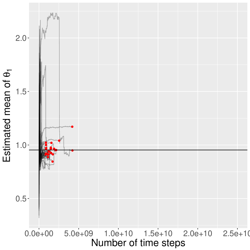
(a) DA-ABC-SMC: $N=500$, $U=100$, $A=100$, $s=0.1$.

(b) DA-ABC-SMC: $N=5000$, $U=100$, $A=100$, $s=0.1$.

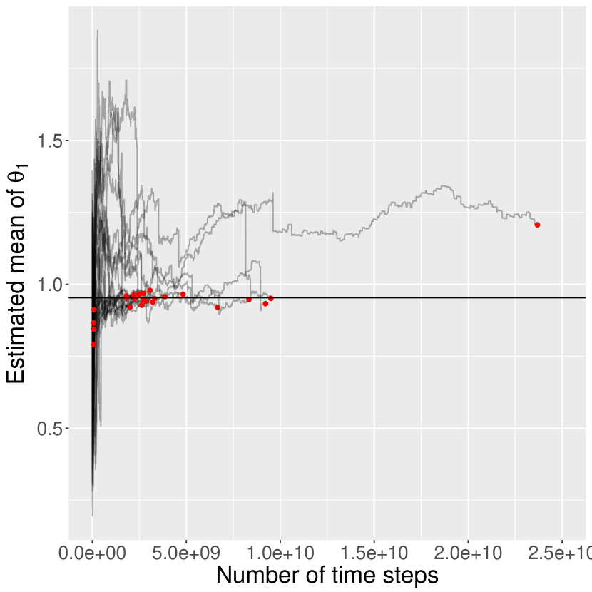
(c) ABC-SMC: $N=200$, $U=100$.

Figure 1: The estimated posterior mean plotted against the total number of time steps used in Euler-Maruyama.

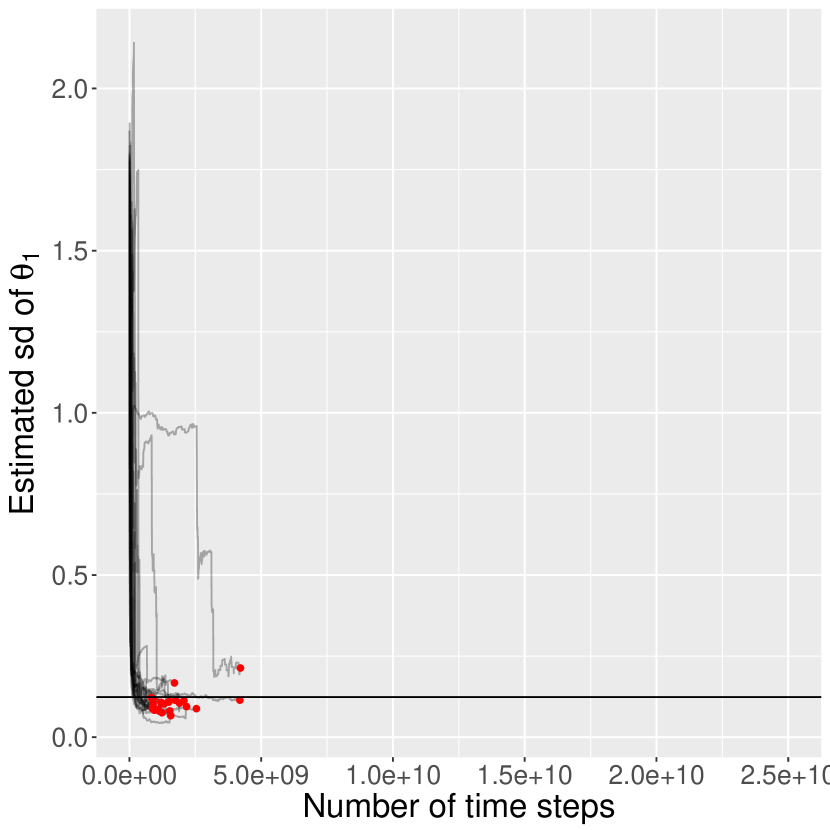
(a) DA-ABC-SMC: $N=500$, $U=100$, $A=100$, $s=0.1$.

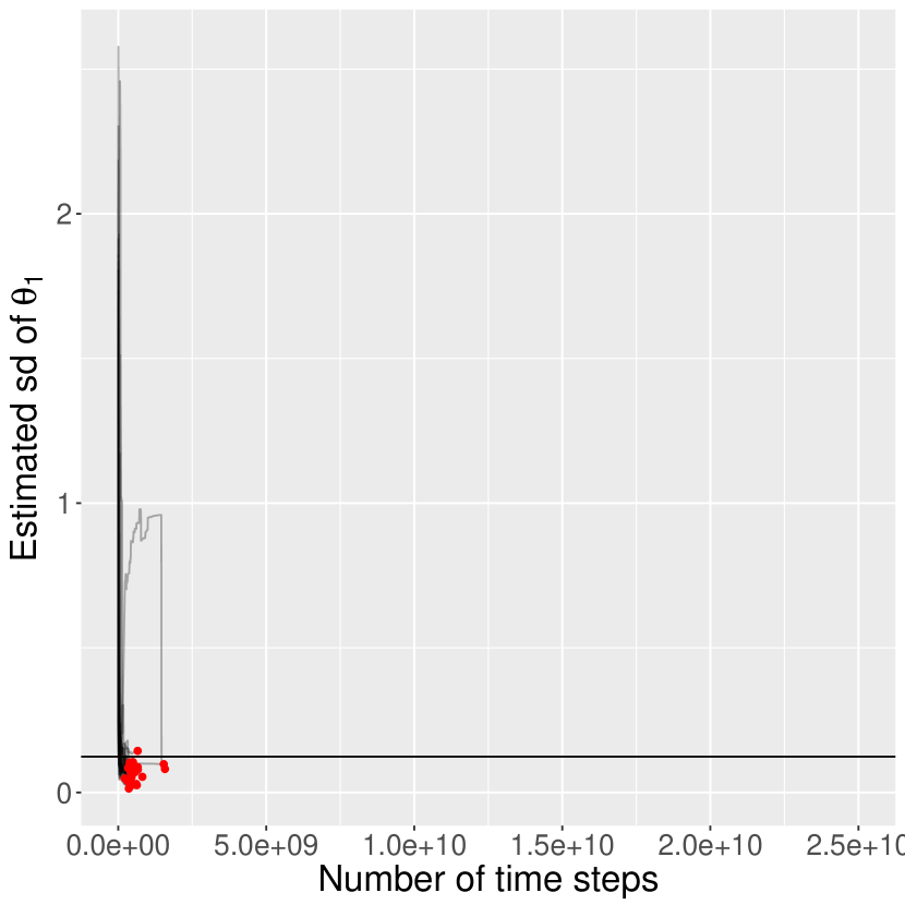
(b) DA-ABC-SMC: $N=5000$, $U=100$, $A=100$, $s=0.1$.

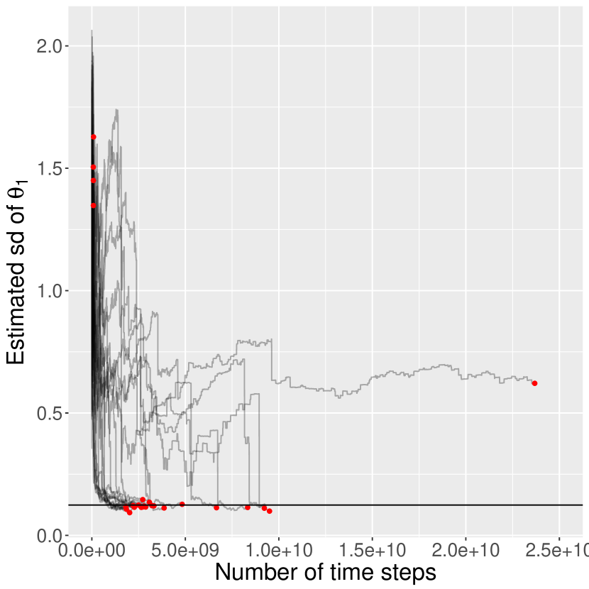
(c) ABC-SMC: $N=200$, $U=100$.

Figure 2: The estimated posterior standard deviation plotted against the total number of time steps used in Euler-Maruyama.

Figures 1 and 2 show, for every run of three methods, the evolution of the sample mean and standard deviation of the particles against the number of time steps of the numerical solver, with the final red dot indicating the estimate from the final distribution (where $\epsilon_{2}=0.15$ was reached). The black line on each plots shows estimated ground truth values estimated using 20 runs of ABC-MCMC of length 5,000 each. We only show the results for $\theta_{1}$ here, since the results for the other parameters are comparable in terms of how they illustrate the properties of the algorithms. The method on the left is DA-ABC-SMC with $N=500$ and $U=A=100$; in the middle is DA-ABC-SMC with $N=5000$ and $U=A=100$; and on the right is ABC-SMC with $N=200$ and $U=100$. We observe that whilst ABC-SMC takes significantly more steps to converge to the target distribution, the estimates of the mean and standard deviation have a relatively low variance. The DA-ABC-SMC approaches converge much faster, but result in estimates that are usually further from the ground truth. In addition, both DA-ABC-SMC approaches appear to underestimate the posterior standard deviation, with this effect becoming more pronounced when $N$ is larger. This result suggests that choosing $N$ too large (resulting in $A/N$ being small) can result in a DA proposal that is too concentrated compared to the target. To further elaborate on this important point, as the ratio $A/N$ decreases, the first stage of the DA leads to a very poor proposal - this is because the particles that make it through to the second stage of the DA step are those that have simulations that result in the very smallest distance to the observed data. The effect is to make the DA proposal too concentrated around the mode of the posterior yielded by the fast approximation.

Tables 1 and 2 summarise the properties of the estimates of the posterior mean and standard deviation from each method. The bias, standard deviation and root mean square error (RMSE) are reported, along with the RMSE$\times\sqrt{\bar{\mathbf{S}}}$, to help compare the errors of methods with different computational costs. The results for some configurations are heavily influenced by poor results from a single run, for example the case of DA-ABC-SMC with $N=1000$, $U=100$, $A=100$ and $s=0.1$. However, based on these tables and the plots of the estimated posterior mean and standard deviation in the appendix, there is evidence to make the following conclusions.

Method	Bias	Std. dev.	RMSE	RMSE$\times\sqrt{\bar{\mathbf{S}}}$
DA-ABC-SMC: $N=500$, $U=100$, $A=100$, $s=0.1$.	0.0033	0.0625	0.0626	2235
DA-ABC-SMC: $N=500$, $U=100$, $A=100$, $s=0.5$.	-0.0047	0.0439	0.0442	1449
DA-ABC-SMC: $N=1000$, $U=100$, $A=100$, $s=0.1$.	0.0659	0.2294	0.2387	6861
DA-ABC-SMC: $N=1000$, $U=100$, $A=100$, $s=0.5$.	-0.0003	0.0381	0.0381	1012
DA-ABC-SMC: $N=1000$, $U=200$, $A=100$, $s=0.1$.	0.0006	0.0559	0.0559	4320
DA-ABC-SMC: $N=1000$, $U=50$, $A=100$, $s=0.1$.	-0.0046	0.0754	0.0756	1232
DA-ABC-SMC: $N=5000$, $U=100$, $A=100$, $s=0.1$.	-0.0097	0.1094	0.1099	2401
DA-ABC-SMC: $N=10000$, $U=100$, $A=100$, $s=0.1$.	-0.0459	0.0703	0.0840	1960
SMC2: $N=100$, $M=100$, $\alpha=0.9$, $s=0.1$.	0.2929	1.2136	1.2485	35065
SMC2: $N=100$, $M=100$, $\alpha=0.99$, $s=0.1$.	0.3261	1.0518	1.1012	55438
SMC2: $N=100$, $M=1000$, $\alpha=0.9$, $s=0.1$.	0.9847	1.6379	1.9111	150838
ABC-SMC: $N=200$, $U=100$.	-0.0092	0.0692	0.0698	3718
ABC-SMC*: $N=200$, $U=100$.	0.0081	0.0583	0.0589	3136

Table 1: Properties of estimators of the posterior mean of $\theta_{1}$. *The final line of the table refers to ABC-SMC where the runs that did not terminate are excluded from the calculation of the statistics.

Method	Bias	Std. dev.	RMSE	RMSE$\times\sqrt{\bar{\mathbf{S}}}$
DA-ABC-SMC: $N=500$, $U=100$, $A=100$, $s=0.1$.	-0.0178	0.0299	0.0348	1242
DA-ABC-SMC: $N=500$, $U=100$, $A=100$, $s=0.5$.	-0.0403	0.0200	0.0450	1476
DA-ABC-SMC: $N=1000$, $U=100$, $A=100$, $s=0.1$.	0.0207	0.2368	0.2377	6833
DA-ABC-SMC: $N=1000$, $U=100$, $A=100$, $s=0.5$.	-0.0488	0.0194	0.0525	1393
DA-ABC-SMC: $N=1000$, $U=200$, $A=100$, $s=0.1$.	-0.0104	0.0275	0.0294	2273
DA-ABC-SMC: $N=1000$, $U=50$, $A=100$, $s=0.1$.	-0.0507	0.0277	0.0578	942
DA-ABC-SMC: $N=5000$, $U=100$, $A=100$, $s=0.1$.	-0.0568	0.0307	0.0645	1410
DA-ABC-SMC: $N=10000$, $U=100$, $A=100$, $s=0.1$.	-0.0621	0.0277	0.0680	1587
ABC-SMC: $N=200$, $U=100$.	0.2321	0.5136	0.5636	30023
ABC-SMC*: $N=200$, $U=100$.	0.0175	0.1105	0.1119	5961

Table 2: Properties of estimators of the posterior standard deviation of $\theta_{1}$. *The final line of the table refers to ABC-SMC where the runs that did not terminate are excluded from the calculation of the statistics.

• Choosing $N$ too large (resulting in $A/N$ being small) can result in a DA proposal that is too concentrated compared to the target, and leads to underestimating the posterior standard deviation.

• Even when $N$ is not large, in this example often DA-ABC-SMC results in a sample that underestimates the standard deviation of the posterior distribution. The likely cause of this is that the DA proposal is too concentrated. This proposal easily generates unique points, thus the tolerance $\epsilon_{2}$ is reduced too quickly, resulting in a poor quality sample. The results from DA-ABC-SMC when $N=1000$, $U=200$, $A=100$ and $s=0.1$, where 200 instead of 100 unique points are required when reducing the tolerance, suggests that when the SMC does not reduce the tolerance as fast (and hence more MCMC moves are made), the estimates of the posterior standard deviation are more accurate.

• DA-ABC-SMC can offer improved performance over ABC-SMC when measured by RMSE scaled by computational cost. This is largely due to its ability to quickly locate the region of highest posterior mass. However, it may not provide a representative sample from the posterior if the DA proposal is not tuned well. In contrast, compared to DA-ABC-SMC, standard ABC-SMC may be extremely slow in converging at all.

• The SMC² approaches tried here do not lead to an improvement over the ABC approaches, due to the low acceptance rate of the particle MCMC moves used in the move step of the SMC sampler (a consequence of the high variance likelihood estimates). In many cases no proposals were accepted at an SMC iteration, leading to a poor quality sample.

5 Applications to doubly intractable distributions

5.1 Background

This section concerns the class of likelihoods that may not be evaluated pointwise due to the presence of an intractable normalising constant, i.e.

$$l\left(y\mid\theta\right)=\frac{\gamma\left(y\mid\theta\right)}{Z\left(\theta\right)},$$

where $\gamma\left(y\mid\theta\right)$ is tractable, but it is not computationally feasible to evaluate the normalising constant $Z\left(\theta\right)$ (also known as the partition function). Such a distribution is known as doubly intractable (Murray et al., 2006) since it is not possible to directly use the Metropolis-Hastings algorithm to simulate from the posterior $\pi\left(\theta\mid y\right)$, due to the presence of $Z\left(\cdot\right)$ in both the numerator and denominator of the acceptance ratio. The most common occurrence of these distributions occurs when $l$ factorises as a Markov random field. The most well-established approaches to inference for these models are the single and multiple auxiliary variable approaches (Møller et al., 2006; Murray et al., 2006) and the exchange algorithm (Murray et al., 2006), which respectively use importance sampling estimates of the likelihood and acceptance ratio to avoid the calculation of the normalising constant. From here on we refer to these as “auxiliary variable methods”. ABC (Grelaud et al., 2009) and synthetic likelihood (Everitt et al., 2017) have also been used for inference in these models. See Stoehr (2017) for a recent, thorough review of the literature.

Previous work, e.g. Friel (2013), suggests that auxiliary variable methods are more effective than ABC for simulating from the posterior $\pi\left(\theta\mid y\right)$ when $l$ has an intractable normalising constant. In the full data ABC case, Everitt et al. (2017) suggest that this is because the multiple auxiliary variable approach may be seen to be a carefully designed non-standard ABC method. However, in this paper we consider the situation in Everitt (2012), where our data $y$ are indirect observations of a latent (hidden) field $x^{h}$, modelled with a joint distribution $p\left(\theta\right)l\left(x^{h}\mid\theta\right)g\left(y\mid x^{h},\theta\right)$ with $l\left(x^{h}\mid\theta\right)$ having an intractable normalising constant. In this case we might expect ABC to become more competitive, or even to outperform other approaches. The most obvious approach is to use data augmentation: using MCMC to simulate from the joint posterior $\pi\left(\theta,x^{h}\mid y\right)$ by alternating simulation from the full conditionals of $\theta$ and $x^{h}$, with the exchange algorithm in the $\theta$ update. Everitt (2012) compares this approach with “exchange marginal particle MCMC”, in which an SMC algorithm is used to integrate out the $x^{h}$ variables at every iteration of an MCMC and finds the particle MCMC approach to be preferable. However, in order to perform well, both of these approaches require efficient simulation from the conditional distribution $\pi\left(x^{h}\mid\theta,y\right)$.

Now compare these “exact” approaches with ABC. In this case, for every $\theta$ we simulate $x^{h}\sim l\left(\cdot\mid\theta\right)$ and $x\sim g\left(\cdot\mid x^{h},\theta\right)$, then use an ABC likelihood that compares $S\left(x\right)$ with $S\left(y\right)$. The $x^{h}$ variables corresponding to a particular $\theta$ variable that are retained in the ABC sample are distributed according to an ABC approximation to $\pi\left(x^{h}\mid\theta,S\left(y\right)\right)$; indeed, in order that the ABC is at all efficient, there must be a reasonable probability that simulated $x^{h}$ is in a region of high probability mass under this distribution. Compared to particle MCMC:

• Standard ABC has the disadvantage that the simulation of $x^{h}$ is, in contrast to particle MCMC, not conditioned on $y$ (although we note recent work in Prangle et al. (2017) in which for some models we may also refine the ABC likelihood by conditioning on $y$).

• ABC has the advantage that a posteriori $x^{h}$ is only conditioned on some statistic $S\left(y\right)$, rather than $y$ as in particle MCMC. This condition is often considerably less stringent. For example, consider the Ising model example described below. When conditioning on $y$, the posterior $\pi\left(x^{h}\mid\theta,y\right)$ is often restricted to relatively small regions of $x^{h}$-space: for individual pixel of $x^{h}$ the posterior mass may be concentrated in a small region in order to match each individual data point. However, when conditioning on $S\left(y\right)$, the posterior $\pi\left(x^{h}\mid\theta,S\left(y\right)\right)$ may have non-negligible mass in many regions of $x^{h}$-space: there are many different configurations of pixels that give rise to similar summary statistics.

In this paper we revisit using ABC on these models, examining the data previously studied in Everitt (2012), and show it is possible to make computational savings using DA-ABC-SMC. We now introduce the cheap simulator that makes this improvement possible. In Markov random field models, exact simulation from $l\left(\cdot\mid\theta\right)$ is either very expensive or intractable. Grelaud et al. (2009) proposes to replace the exact simulator with taking the last point of a long MCMC run, and Everitt (2012) shows that, under certain ergodicity conditions, as the length of this “internal” MCMC goes to infinity, the bias in our ABC posterior sample due to this particular approximation also goes to zero (following ideas in Andrieu and Roberts (2009)). However, empirically one finds that often using only a single MCMC iteration is sufficient to yield a posterior close to the desired posterior. In this paper we propose to use an internal MCMC run of a single iteration as the cheap simulator, and to run the internal MCMC for many iterations (we use 1,000) as the expensive simulator, where the final iteration of the cheap simulator is used as the first iteration of the expensive simulator. The next section presents an application to latent Ising models, with an application to ERGMs in the appendix.

5.2 Latent Ising model

An Ising model is a pairwise Markov random field model on binary variables, each taking values in $\left\{-1,1\right\}$. Its distribution is given by

$$l\left(x^{h}\mid\theta_{x}\right)\propto\exp\left(\theta_{x}\sum_{\left(i,j\right)\in\mathbf{N}}x_{i}^{h}x_{j}^{h}\right),$$

where $\theta_{x}\in\mathbb{R}$, $x_{i}^{h}$ denotes the $i$-th random variable in $x^{h}$ and $\mathbf{N}$ is a set defining pairs of nodes that are “neighbours”. We consider the case where the neighbourhood structure is given by a regular 2-dimensional grid. Our data $y$ are noisy observations of this $x^{h}$ field: the $i$-th variable in $y$ has distribution

$$g\left(y_{i}\mid x_{i}^{h},\theta_{y}\right)\propto\exp\left(\theta_{y}y_{i}x_{i}^{h}\right),$$

as in Everitt (2012) (with the normalising constant being intractable). We used independent Gaussian priors on $\theta_{x}$ and $\theta_{y}$, each with mean 0 and standard deviation 5. Our DA-ABC-SMC algorithm used $U=A=100$, and we examined different values of $N$. A single site Gibbs sampler was used to simulate from the likelihood, with the expensive simulator using the final point of 1,000 sweeps of the Gibbs sampler. The MCMC proposal was taken to be a Gaussian distribution centred at the current particle, with covariance given by the sample covariance of the particles from the previous iteration. We used a single statistic in the ABC: the number of equivalently valued neighbours $S\left(y\right)=\sum_{\left(i,j\right)\in\mathbf{N}}y_{i}y_{j}$ (noting that this is not sufficient, but that the particle MCMC results in Everitt (2012) indicate that this does not have a large impact on the posterior). The distance metric used in ABC on the summary statistics was the absolute value of the difference.

We used the same $10\times 10$ grid of data as was studied in Everitt (2012), shown in figure 3(a), which was generated from the model using $\theta_{x}=\theta_{y}=0.1$. These parameter values represent a relatively weak interaction between neighbouring pixels, and also quite noisy observations. On a grid of this size, there is ambiguity as to whether this data may have been generated with either one or both of $\theta_{x}$ and $\theta_{y}$ being small, giving a posterior distribution shaped like a cross, similar to that shown in figure 3(c). Figure 3(c) gives an example of a DA proposal, i.e. points that pass the first stage of the DA-MCMC, from the early stages of a run of DA-ABC-SMC. We observe how this distribution would be a suitable independent MCMC proposal for the posterior.

All of our empirical results were generated using R (R Core Team, 2019), and the R packages ggplot2 (Wickham, 2016), matlab (Roebuck, 2014) and mvtnorm (Genz and Bretz, 2009) were used. We ran DA-ABC-SMC for several values of $N$, and compared the results with standard ABC-SMC using all of the same algorithmic choices, with $N=200$ and $U=100$. The standard ABC-SMC algorithm used the expensive simulator, i.e. 1,000 iterations of the internal Gibbs sampler. In algorithms we terminated the method when $\epsilon_{2}=0$, or after 500 SMC iterations, whichever was sooner. We focus on studying the total computational effort expended in each algorithm, measured by the total number of sweeps $\mathbf{S}$ of the internal Gibbs sampler, and on the mean and standard deviation of the Euclidean distance $\rho$ of the parameter vector $(\theta_{x},\theta_{y})$ from the origin.

We ran the algorithm with several different values of $N$, and two different cheap simulators: the first where only a single sweep of the Gibbs sampler is used ($B=1$); the second using the final point of 5 sweeps of the Gibbs sampler ($B=5$). Each configuration was run 30 times. We chose $N$ such that in most cases the computational cost was dominated by the expensive simulations in the second stage of the DA, although when $N=50,000$ and $B=5$ the cost of the first stage dominated. Figure 3(b) shows gives an example showing the evolution of $\epsilon_{2}$ against the total number of sweeps of the Gibbs sampler for several different configurations. We see that all configurations of the DA approach appear to have a significantly lower cost than standard ABC-SMC: in all cases the DA approach reaches $\epsilon_{2}=0$ whereas the ABC-SMC reaches $\epsilon_{2}=2$.

Table 3 shows properties of estimates of the mean and standard deviation posterior on $\rho$. The estimates from ABC-SMC are based on the output of the 500th iteration of the SMC, where in all runs $\epsilon_{2}=2$. we observe that we obtain lower variance estimates from ABC-SMC than from DA-ABC-SMC, but at a higher cost. This cost may be significantly higher if we wish to reduce $\epsilon_{2}$ to 0, as is achieved in all cases by DA-ABC-SMC. As in the previous section, we note that using a large value of $N$ appears to lead to poor results; it appears likely that the standard deviation of the posterior is being underestimated.

Method	Mean	sd	sd$\times\sqrt{\bar{\mathbf{S}}}$	Mean	sd	sd$\times\sqrt{\bar{\mathbf{S}}}$	$\bar{\mathbf{S}}$
DA $N=500$, $B=1$	3.3776	0.5517	11579	2.5534	0.4121	8649	$4.41\times 10^{5}$
DA $N=1000$, $B=1$	3.6168	1.2165	21352	2.4516	0.7231	12693	$3.08\times 10^{5}$
DA $N=5000$, $B=1$	3.7702	1.6169	26462	1.7376	0.9840	16104	$2.68\times 10^{5}$
DA $N=10000$, $B=1$	3.7532	2.0874	33747	1.9016	0.8581	13874	$2.61\times 10^{5}$
DA $N=50000$, $B=1$	3.2808	2.4644	44738	1.5644	1.0555	19162	$3.30\times 10^{5}$
DA $N=500$, $B=5$	3.8090	1.1143	22445	2.7266	0.6132	12353	$4.06\times 10^{5}$
DA $N=1000$, $B=5$	3.4027	0.9633	16572	2.3664	0.8668	14911	$2.96\times 10^{5}$
DA $N=5000$, $B=5$	3.5438	2.0486	35046	1.8708	0.6549	11205	$2.93\times 10^{5}$
DA $N=10000$, $B=5$	3.6596	1.7692	31444	1.7683	0.9247	16435	$3.16\times 10^{5}$
DA $N=50000$, $B=5$	3.8090	2.0645	43305	1.4834	1.0414	21845	$4.40\times 10^{5}$
ABC-SMC $N=200$	3.7580	0.3659	31000	2.9472	0.2501	21188	$7.18\times 10^{6}$

Table 3: The mean and standard deviation of the estimated posterior mean (columns 2-4) and standard deviation (columns 5-7) of $\rho$, and the median number $\bar{\mathbf{S}}$ of sweeps of the Gibbs sampler $\bar{\mathbf{S}}$. All rows refer to DA approaches, except the last, which is standard ABC-SMC.

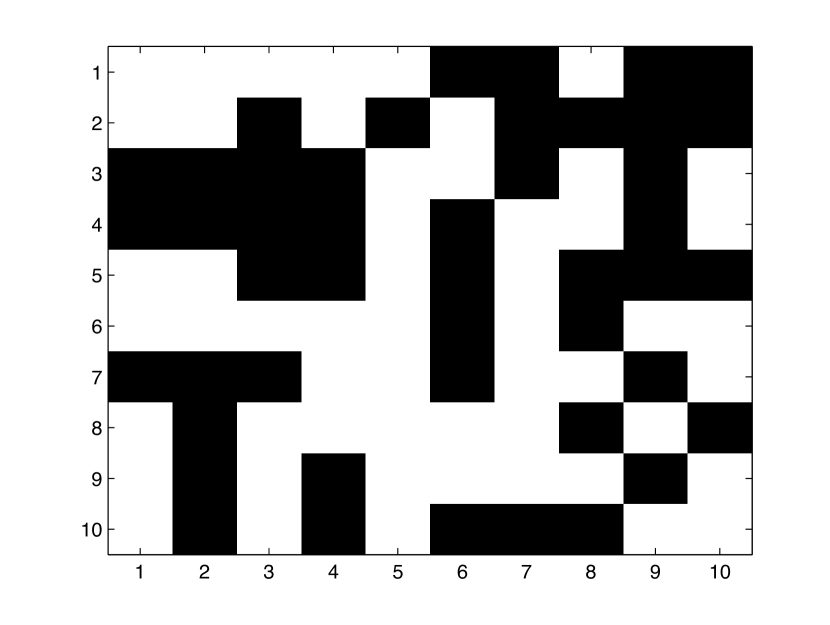
(a) Observed data.

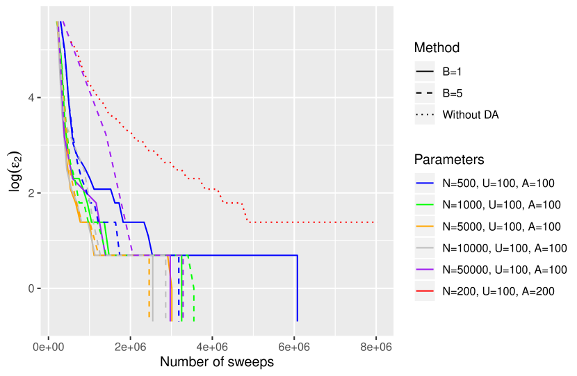
(b) $\log\left(\epsilon_{2,t}\right)$ plotted against the number of sweeps of the Gibbs sampler. When $\epsilon_{2,t}=0$ we plot $\log\left(\epsilon_{2,t}\right)=-\log\left(2\right)$.

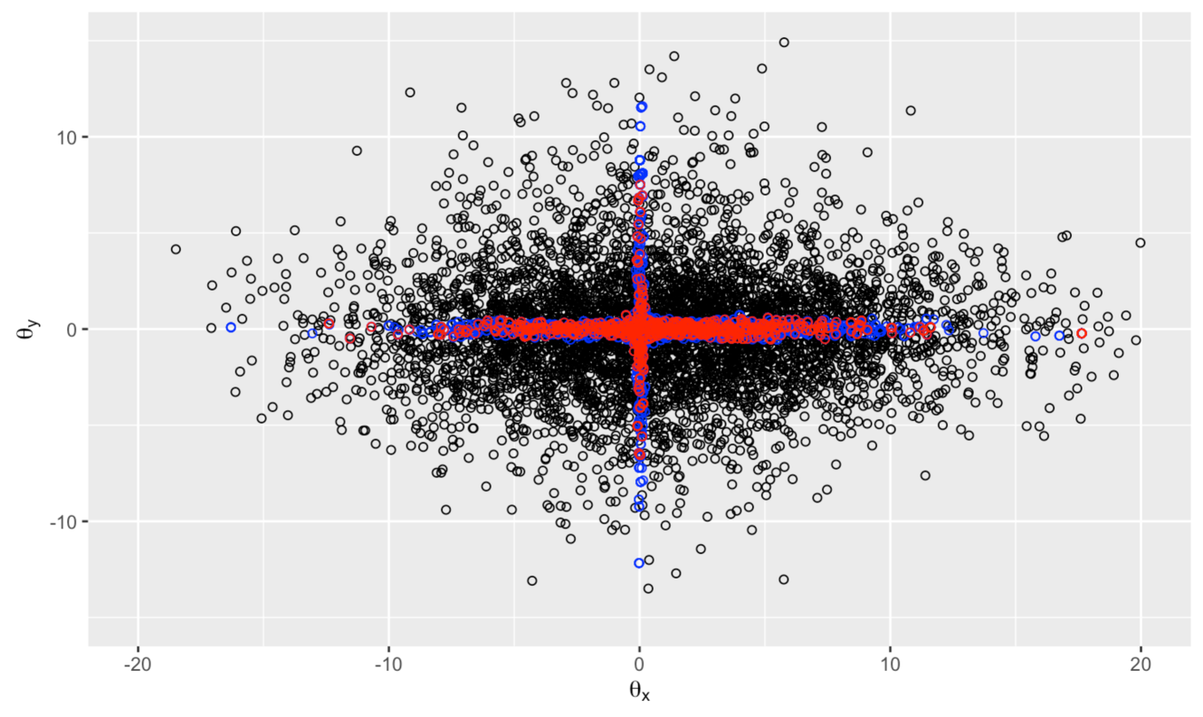
(c) Points drawn at a single iteration of DA-ABC-SMC with $N=5000$, $A=U=1000$. Proposed points (black) are plotted alongside points from the DA proposal (red), with $\epsilon_{1}=68$, and points from the posterior (blue), with $\epsilon_{2}=8$.

Figure 3: DA-ABC-SMC applied to the latent Ising model.

6 Conclusions

In this paper we introduced DA-ABC-SMC as a means for reducing the computational cost of ABC-SMC in the case of an expensive simulator, through using a DA-ABC-MCMC move, in which a cheap simulator is used to “screen” the candidate values of proposed parameters so that less effort needs to be used running the expensive simulator. This cheap simulator may be completely independent of the expensive simulator, but preferably the expensive simulator may be conditioned on the output of the cheap simulator. The tolerance for the cheap simulator is chosen adaptively with DA-ABC-SMC, giving an algorithm that only has three relatively easy to choose tuning parameters. The key factor in the performance of the algorithm is the DA proposal, i.e. the distribution of the particles that pass the first stage of DA. For this proposal to be useful, the cheap simulator needs to produce a posterior centred around the same values as the expensive simulator, and the total number of particles $N$ in the DA-ABC-SMC needs to be chosen appropriately. The empirical results suggest that there is a trade-off in choosing the size of $N$: large values result in the largest computational saving, but can produce a DA proposal that is too concentrated which can result in a poor sample from the posterior. For smaller values of $N$ the DA proposal is usually more suitable, and can result in computational savings compared to ABC-SMC.

Section 4 illustrates that DA-ABC-SMC shows promise for using ABC for inference in ODE or SDE models, where a numerical method is used to simulate from the model. Section 5 revisits the idea of using ABC for inference in latent Markov random field models, and suggests an approach that in some cases reduces the computational cost of ABC-SMC by using short runs of MCMC to simulate from the model. Future work might extend the approach to ABC methods that do not use an indicator kernel, use the adaptive tuning of the first stage of DA outside of the ABC context (along with an investigation of any bias this adaptation may introduce), or aim to improve the automation of the design of the DA proposal, which is often too concentrated.

Appendix A ABC-MCMC and ABC-SMC

This section derives the ABC-MCMC algorithm (section A.1), and the ABC-SMC of Del Moral et al. (2012a) (section A.2).

A.1 ABC-MCMC and early rejection

ABC-MCMC Marjoram et al. (2003) can be derived by applying standard Metropolis-Hastings (MH) to the target

$$\pi\left(\theta,x\mid y\right)\propto p\left(\theta\right)l\left(x\mid\theta\right)P_{\epsilon}\left(y\mid x\right)$$ (14)

(omitting the dependence of the target on $\epsilon$ to keep the notation consistent throughout the paper). ABC-MCMC uses the proposal $q\left(\theta^{*}\mid\theta\right)l\left(x^{*}\mid\theta^{*}\right)$ on the pair $(\theta,x)$, giving the acceptance probability

$$\alpha\left((\theta,x),(\theta^{*},x^{*})\right) = \frac{p\left(\theta^{*}\right)l\left(x^{*}\mid\theta^{*}\right)P_{\epsilon}\left(y\mid x^{*}\right)}{p\left(\theta\right)l\left(x\mid\theta\right)P_{\epsilon}\left(y\mid x\right)}\frac{q\left(\theta\mid\theta^{*}\right)l\left(x\mid\theta\right)}{q\left(\theta^{*}\mid\theta\right)l\left(x^{*}\mid\theta^{*}\right)}$$ (15)

$$= \frac{p\left(\theta^{*}\right)P_{\epsilon}\left(y\mid x^{*}\right)}{p\left(\theta\right)P_{\epsilon}\left(y\mid x\right)}\frac{q\left(\theta\mid\theta^{*}\right)}{q\left(\theta^{*}\mid\theta\right)}.$$ (16)

The cancellation of the likelihood terms allows this algorithm to be implemented.

A.1.1 Indicator kernels and early rejection

In ABC a common choice for the kernel $P_{\epsilon}$ is $P_{\epsilon}\left(y\mid x\right)\propto\mathbb{I}\left(d\left(y,x\right)<=\epsilon\right)$, where $d$ is a distance metric. We now consider the implications of using this kernel on the ABC-MCMC acceptance probability in the preceding section. Firstly, we must consider the possibility that the denominator in the ratio is equal to 0, due to having $d\left(y,x\right)>\epsilon$. The general MH framework of Tierney (1998) (see the main paper) dictates that the acceptance probability in this case should be 0: the practical implications of this are that one must ensure that the initial value of $x$ satisfies $d\left(y,x\right)<=\epsilon$, or the chain will never move from its starting point (in practice instead often different values of $(\theta,x)$ are explored until $d\left(y,x\right)<=\epsilon$ is satisfied, with this initial exploration being discarded). Therefore, we may always assume that $d\left(y,x\right)<=\epsilon$ after the chain is initialised and hence the acceptance probability may be written as

$$\alpha\left((\theta,x),(\theta^{*},x^{*})\right)=\begin{cases}\frac{p\left(\theta^{*}\right)q\left(\theta\mid\theta^{*}\right)}{p\left(\theta\right)q\left(\theta^{*}\mid\theta\right)}&\text{if }d\left(y,x^{*}\right)<=\epsilon\\ 0&\text{otherwise}\end{cases}.$$ (17)

Let $u$ be the uniformly distributed random number in $[0,1]$ generated in order implement the accept-reject step. Picchini and Forman (2016) note that a rejection will always occur if

$$u>\frac{p\left(\theta^{*}\right)q\left(\theta\mid\theta^{*}\right)}{p\left(\theta\right)q\left(\theta^{*}\mid\theta\right)}$$ (18)

thus this condition may be checked before $x^{*}$ is simulated from the likelihood. If the proposed point is not rejected after this first step, $x^{*}$ is simulated, and the proposal is accepted if $d\left(y,x^{*}\right)<=\epsilon$. The consequence of this idea is that for $\theta^{*}$ that have a small probability under the prior, we have an “early rejection” that avoids the (potentially expensive) cost of simulation. The computational savings of this approach will only be significant if the posterior is not too different from the prior.

For clarity, pseudo-code for the early rejection method is given in algorithm 3.

Algorithm 3 A single iteration of early rejection ABC-MCMC.

Inputs: Current value of $\theta$.
      Outputs: Proposed value $\theta^{*}$ and accept/reject decision for this proposed value.

$u\sim\mathcal{U}\left(0,1\right)$

$\theta^{*}\sim q\left(\cdot\mid\theta\right)$

if $u<1\wedge\frac{p\left(\theta^{*}\right)q\left(\theta\mid\theta^{*}\right)}{p\left(\theta\right)q\left(\theta^{*}\mid\theta\right)}$  then

     $x^{*}\sim l\left(\cdot\mid\theta^{*}\right)$

     if  $d\left(y,x^{*}\right)<\epsilon$  then

         Accept $\theta^{*}$.

     else

         Reject $\theta^{*}$.

     end if

else

     Reject $\theta^{*}$.

end if

A.2 ABC-SMC

Recall from the main paper the weight update used in an SMC sampler (Del Moral et al., 2006) when using a sequence of targets $\pi_{t}$, an MCMC move for the “move” step, and where the SMC sampler backwards kernel is the reverse of this MCMC kernel:

$$\tilde{w}_{t+1}^{(i)} = w_{t}^{(i)}\frac{\pi_{t+1}\left(\theta_{t}^{(i)}\right)}{\pi_{t}\left(\theta_{t}^{(i)}\right)}.$$ (19)

The sequence of targets used in the ABC-SMC sampler of Del Moral et al. (2012a) is given by

$$\pi_{t}\left(\theta_{t},x_{t}\mid y\right)\propto p\left(\theta_{t}\right)l\left(x_{t}\mid\theta_{t}\right)P_{\epsilon_{t}}\left(y\mid x_{t}\right),$$ (20)

for $t=1:T$. We saw in the previous section that the ABC-MCMC kernel is a valid MCMC kernel targeting $\pi_{t}\left(\theta_{t},x_{t}\mid y\right)$. Choosing the SMC sampler backwards kernel to be the reverse of this MCMC kernel we obtain

$$\tilde{w}_{t+1} = w_{t}\frac{p\left(\theta_{t}\right)l\left(x_{t}\mid\theta_{t}\right)P_{\epsilon_{t+1}}\left(y\mid x_{t}\right)}{p\left(\theta_{t}\right)l\left(x_{t}\mid\theta_{t}\right)P_{\epsilon_{t}}\left(y\mid x_{t}\right)}$$ (21)

$$= w_{t}\frac{P_{\epsilon_{t+1}}\left(y\mid x_{t}\right)}{P_{\epsilon_{t}}\left(y\mid x_{t}\right)}.$$ (22)

In the case of indicator kernels, this weight update becomes

$$\tilde{w}_{t+1}=w_{t}\mathbb{I}\left(d\left(y,x_{t}\right)<\epsilon_{t+1}\right),$$

and early rejection may be used in the ABC-MCMC move. Early rejection may provide a significant computational saving in the early stages of the SMC, since the target is likely to be close to the prior.

Appendix B Derivation of DA-ABC-MCMC and DA-ABC-SMC

B.1 DA-ABC-MCMC

We present a derivation of DA-ABC-MCMC, using the notation from the main paper. As in the previous sections, the extended state space view of ABC-MCMC is used, where the move is seen to be a Metropolis-Hastings move on the space $\left(\theta,x_{1}\right)$, with $\theta^{*}$ proposed via $q\left(\cdot\mid\theta\right)$ and $x_{1}^{*}$ via $l_{1}\left(\cdot\mid\theta^{*}\right)$. We may view the move as being on the space $\left(\theta,x_{1},x_{2}\right)$, with target proportional to

$$p\left(\theta^{*}\right)l_{1}\left(x_{1}\mid\theta\right)l_{2}\left(x_{2}\mid x_{1},\theta\right)P_{\epsilon_{2}}\left(y\mid x_{1},x_{2}\right)$$

with $x_{2}^{*}$ being proposed via $l_{2}\left(\cdot\mid x_{1}^{*},\theta^{*}\right)$. We will see that in practice this simulation does not need to be performed at the first stage (this construction is essentially the same as in Sherlock et al. (2017)). The acceptance probability at the first stage is

$$\alpha_{1} = \min\left\{1,\frac{p\left(\theta^{*}\right)l_{1}\left(x_{1}^{*}\mid\theta^{*}\right)P_{\epsilon_{1}}\left(y_{1}\mid x_{1}^{*}\right)l_{2}\left(x_{2}^{*}\mid x_{1}^{*},\theta^{*}\right)}{p\left(\theta\right)l_{1}\left(x_{1}\mid\theta\right)P_{\epsilon_{1}}\left(y_{1}\mid x_{1}\right)l_{2}\left(x_{2}\mid x_{1},\theta\right)}\frac{q\left(\theta\mid\theta^{*}\right)l_{1}\left(x_{1}\mid\theta\right)l_{2}\left(x_{2}\mid x_{1},\theta\right)}{q\left(\theta^{*}\mid\theta\right)l_{1}\left(x_{1}^{*}\mid\theta^{*}\right)l_{2}\left(x_{2}^{*}\mid x_{1}^{*},\theta^{*}\right)}\right\}$$

$$= \min\left\{1,\frac{p\left(\theta^{*}\right)P_{\epsilon_{1}}\left(y_{1}\mid x_{1}^{*}\right)}{p\left(\theta\right)P_{\epsilon_{1}}\left(y_{1}\mid x_{1}\right)}\frac{q\left(\theta\mid\theta^{*}\right)}{q\left(\theta^{*}\mid\theta\right)}\right\}.$$

We observe that the marginal distribution of the target we have used is the ABC posterior with $l_{1}$, $\epsilon_{1}$ and $y_{1}$.

Using delayed acceptance, as described in the main paper, the acceptance probability at the second stage is

$$\alpha_{2} = \min\left\{1,\frac{p\left(\theta^{*}\right)l_{1}\left(x_{1}^{*}\mid\theta^{*}\right)l_{2}\left(x_{2}^{*}\mid x_{1}^{*},\theta^{*}\right)P_{\epsilon_{2}}\left(y\mid x_{1}^{*},x_{2}^{*}\right)}{p\left(\theta\right)l_{1}\left(x_{1}\mid\theta\right)l_{2}\left(x_{2}\mid x_{1},\theta\right)P_{\epsilon_{2}}\left(y\mid x_{1},x_{2}\right)}\frac{p\left(\theta\right)l_{1}\left(x_{1}\mid\theta\right)P_{\epsilon_{1}}\left(y_{1}\mid x_{1}\right)l_{2}\left(x_{2}\mid x_{1},\theta\right)}{p\left(\theta^{*}\right)l_{1}\left(x_{1}^{*}\mid\theta^{*}\right)P_{\epsilon_{1}}\left(y_{1}\mid x_{1}^{*}\right)l_{2}\left(x_{2}^{*}\mid x_{1}^{*},\theta^{*}\right)}\right\}$$

$$= \min\left\{1,\frac{P_{\epsilon_{2}}\left(y\mid x_{1}^{*},x_{2}^{*}\right)}{P_{\epsilon_{2}}\left(y\mid x_{1},x_{2}\right)}\frac{P_{\epsilon_{1}}\left(y_{1}\mid x_{1}\right)}{P_{\epsilon_{1}}\left(y_{1}\mid x_{1}^{*}\right)}\right\}.$$

B.2 DA-ABC-SMC

We now justify the weight update for the DA-ABC-SMC method described in the main paper. The target distribution used at iteration $t$ is proportional to

$$p\left(\theta_{t}\right)l_{1}\left(x_{1,t}\mid\theta_{t}\right)l_{2}\left(x_{2,t}\mid x_{1,t},\theta_{t}\right)P_{\epsilon_{2,,t}}\left(y\mid x_{1,t},x_{2,t}\right).$$

Using the same approach as in section A.2, we see that the weight update for each particle is given by

$$\tilde{w}_{t+1} = w_{t}\frac{p\left(\theta_{t}\right)l_{1}\left(x_{1,t}\mid\theta_{t}\right)l_{2}\left(x_{2,t}\mid x_{1,t},\theta_{t}\right)P_{\epsilon_{2,,t+1}}\left(y\mid x_{1,t},x_{2,t}\right)}{p\left(\theta_{t}\right)l_{1}\left(x_{1,t}\mid\theta_{t}\right)l_{2}\left(x_{2,t}\mid x_{1,t},\theta_{t}\right)P_{\epsilon_{2,,t}}\left(y\mid x_{1,t},x_{2,t}\right)}$$

$$= w_{t}\frac{P_{\epsilon_{2,,t+1}}\left(y\mid x_{1,t},x_{2,t}\right)}{P_{\epsilon_{2,,t}}\left(y\mid x_{1,t},x_{2,t}\right)}.$$

B.2.1 Using indicator kernels

In this section we consider the situation when $P_{\epsilon_{1,t}}$ is chosen to be an indicator function; i.e. $P_{\epsilon_{1,t}}\left(y_{1,t}\mid x_{1,t}^{*}\right)\propto\mathbb{I}\left(d\left(y_{1,t},x_{1,t}^{*}\right)<=\epsilon_{1,t}\right)$, where $d$ is a distance metric. In this case when specifying our acceptance probabilities we need to account for our target distributions having zero density in some parts of the space. We follow the framework of Tierney (1998), in which for a target $\pi(\theta)$ and proposal $q$, the MH acceptance probability is written as

$$\alpha=\begin{cases}\min\left\{1,\frac{\pi\left(\theta^{*}\right)q\left(\theta\mid\theta^{*}\right)}{\pi\left(\theta\right)q\left(\theta^{*}\mid\theta\right)}\right\}&\left(\theta,\theta^{*}\right)\in R,\\ 0&\left(\theta,\theta^{*}\right)\notin R,\end{cases}$$

where $R=\left\{\left(\theta,\theta^{*}\right)\mid\pi\left(\theta^{*}\right)q\left(\theta\mid\theta^{*}\right)>0,\pi\left(\theta\right)q\left(\theta^{*}\mid\theta\right)>0\right\}$. Thus, at the $t$-th iteration of the SMC the acceptance probability at the first stage of the delayed acceptance is

$$\alpha_{1,t}=\begin{cases}\min\left\{1,\frac{p\left(\theta_{t}^{*}\right)}{p\left(\theta_{t}\right)}\frac{q\left(\theta_{t}\mid\theta_{t}^{*}\right)}{q\left(\theta_{t}^{*}\mid\theta_{t}\right)}\right\}&d\left(y_{1,t},x_{1,t}\right),d\left(y_{1,t},x_{1,t}^{*}\right)<\epsilon_{1,t},\\ 0&\mbox{otherwise.}\end{cases}.$$ (23)

As in Picchini and Forman (2016), we may perform the first stage of delayed acceptance in two stages, which we will refer to as steps 1a and 1b, such that some simulations from $l_{1}$ may be avoided. At step 1a, $\theta_{t}^{*}$ is simulated from $q\left(\cdot\mid\theta_{t}\right)$ and an accept-reject step is performed using the acceptance probability

$$\alpha_{1\mbox{a},t}=\min\left\{1,\frac{p\left(\theta_{t}^{*}\right)}{p\left(\theta_{t}\right)}\frac{q\left(\theta_{t}\mid\theta_{t}^{*}\right)}{q\left(\theta_{t}^{*}\mid\theta_{t}\right)}\right\}.$$

At step 1b, $x_{1,t}^{*}$ is simulated from $l_{1}\left(\cdot\mid\theta_{t}^{*}\right)$ and the entire move $\left(\theta_{t}^{*},x_{1,t}^{*}\right)$ is accepted (to be used in stage 2) with probability

$$\alpha_{1b,t}=\begin{cases}1&d\left(y_{1,t},x_{1,t}\right),d\left(y_{1,t},x_{1,t}^{*}\right)<\epsilon_{1,t}\\ 0&\mbox{otherwise}\end{cases}.$$ (24)

Splitting the first stage into two substages could itself be seen as a form of delayed acceptance, but its acceptance rate is the same as the single step implementation since it simply uses the fact that $\mathbb{I}\left(d\left(y_{1,t},x_{1,t}^{*}\right)<\epsilon_{1,t}\right)$ is either 1 or 0 in order to reorganise the single step calculation in a computationally efficient way.

The acceptance probability at the second stage is

$$\alpha_{2,t}=\begin{cases}1&d\left(y_{1,t},x_{1,t}\right),d\left(y_{1,t},x_{1,t}^{*}\right)<\epsilon_{1,t}\mbox{ and }d\left(y,x_{2,t}\right),d\left(y,x_{2,t}^{*}\right)<\epsilon_{2,t}\\ 0&\mbox{otherwise}\end{cases},$$

which may be seen directly from the description of DA from the main paper with the appropriate choices of $\pi_{2}$ and $K_{1}$. Note that $d\left(y,x_{2,t}\right)<\epsilon_{2,t}$ must be true for the particle to have non-zero weight, and $d\left(y_{1,t},x_{1,t}\right),d\left(y_{1,t},x_{1,t}^{*}\right)<\epsilon_{1,t}$ must be satisfied to reach the second stage of DA, thus in practice we use

$$\alpha_{2,t}=\begin{cases}1&d\left(y,x_{2,t}^{*}\right)<\epsilon_{2,t},\\ 0&\mbox{otherwise.}\end{cases}$$

Appendix C Lotka-Volterra model

C.1 Full details of methods

All of our empirical results were generated using R (R Core Team, 2019). We study the data “LVPerfect” in the R package smfsb (Wilkinson, 2018) (the numerical methods for simulating from the likelihood are also taken from this package), previously studied in Wilkinson (2011). In this data the simulation starts with initial populations $X=50$ and $Y=100$, and has 30 time units, with the values of $X$ and $Y$ being recorded every 2 time units, resulting in 16 data points in each of the two time series. Our prior follows that in Wilkinson (2011), being uniform in the $\log$ domain. Specifically we use

$$p\left(\log\left(\theta\right)\right)\propto\prod_{i=1}^{3}\mathcal{U}\left(\log\left(\theta_{i}\right)\mid\text{lower}=-6,\text{upper}=2\right).$$

Our ABC approach follows that in Wilkinson (2011); Papamakarios and Murray (2016): as summary statistics we use a 9-dimensional vector composed of the mean, $\log$ variance and first two autocorrelations of each time series, together with the cross-correlation between them. These statistics were normalised by the standard deviation of the statistics determined by a pilot run, precisely as in Wilkinson (2011). The distance between the summary statistics used in ABC was taken to be the Euclidean norm between the normalised statistic vectors. In all our ABC algorithms we used a final tolerance $\log(\epsilon_{2})=\log(0.15)\approx-1.89712$. Reducing the tolerance below this level does not appear to have a large impact on the posterior distribution.

We used DA-ABC-SMC with a variety of choices of $U$, $A$ and $N$, and two different choices of the Euler-Maruyama step size $s$ in the cheap simulator $s=0.5$ and $s=0.1$, both of which result in very rough approximations of the dynamics. We compared these approaches with standard ABC-SMC, with $N=200$ particles and a sequence of tolerances selected such that $U=100$ unique particles are retained at each iteration, and also “ground truth” for the posterior expectation and standard deviation of the parameters found using a long run ($10^{5}$ iterations) of ABC-MCMC. We also compared our approach with a method based on the SMC²-style approach of Duan and Fulop (2015). This approach uses the same SMC-based likelihood estimate (with $M$ particles) as particle MCMC (Wilkinson, 2011), but embeds this within an SMC sampler rather than a pseudo-marginal MCMC chain. The sequence of distributions in the “external” SMC sampler is given by raising the likelihood estimate to a power: beginning with 0 and ending with 1 (so that the final distribution is the true posterior). The posterior targeted by this method is the same as in particle MCMC. We used the same model as in the particle MCMC of Wilkinson (2011): specifically we used a normal distribution with mean 0 and standard deviation 10 as the measurement model at each time step. Wilkinson (2011) shows that the posterior obtained using this model has a much smaller standard deviation compared to the one obtained when using ABC, therefore when comparing the SMC² approach with ABC, we only compared the posterior mean (bearing in mind that this is also slightly different between the two cases). In order that the computational cost is comparable with the ABC approaches, we use a DA move within the method of Duan and Fulop (2015). Full details of this method follow.

Algorithm 4 gives the SMC sampler of Duan and Fulop (2015). This method is adapted so that the sequence of powers to which the likelihood estimates are raised is determined adaptively, by using a bisection search to find the power such that the conditional effective sample size (CESS) (Zhou et al., 2016) is $\alpha N$ (where $\alpha$ is a proportion). The CESS is defined as

$$\text{CESS}=\frac{N\left(\sum_{i=1}^{N}w_{t+1}^{(i)}\omega_{t}^{(i)}\right)^{2}}{\sum_{i=1}^{N}w_{t+1}^{(i)}\left(\omega_{t}^{(i)}\right)^{2}}$$

where $\omega^{(i)}$ is the incremental weight for the $i$th particle (the factor by which we multiply $w_{t}^{(i)}$ by in order to obtain $\tilde{w}_{t+1}^{(i)}$.

Algorithm 4 The SMC sampler of Duan and Fulop (2015), with adaptation to choose the sequence of distributions.

Inputs: Number of particles $N$, the proportion $\alpha$ used in the adaptive approach to choosing the sequence of distributions, the proportion $\beta$ used in resampling, prior $p$, particle filtering parameters for estimating $l$ (including the number of particles $M$).
      Outputs: Particles $\left\{\left(\theta^{(i)}_{t},x^{(i)}_{t}\right)\right\}_{i=1}^{N}$ and weights $\left\{w_{t}^{(i)}\right\}_{i=1}^{N}$ for all $t$.

for $i=1:N$ do

     $\theta^{(i)}_{0}\sim p\left(\cdot\right)$

     Run a particle filter to find the likelihood estimate $\hat{l}^{(i)}_{0}$ at $\theta^{(i)}_{0}$.

     $w^{(i)}_{0}=1/N$

end for

$\tau_{0}=0$, $t=0$.

while $\tau_{t}<1$ do

     Use bisection to choose $\tau_{t+1}$ s.t. the CESS is $\alpha N$.

     for $i=1:N$ do

         $\tilde{w}_{t+1}^{(i)}=w_{t}^{(i)}(\hat{l}^{(i)}_{t})^{(\tau_{t+1}-\tau_{t})}$

     end for

     Normalise $\left\{\tilde{w}_{t+1}\right\}_{i=1}^{N}$ to give normalised weights $\left\{w_{t+1}\right\}_{i=1}^{N}$.

     Perform resampling if the ESS falls below $\beta N$.

     for $i=1:N$ do

         $\theta^{(i)}_{t+1}=\theta^{(i)}_{t}$, $\hat{l}^{(i)}_{t+1}=\hat{l}^{(i)}_{t}$

         $\left(\theta^{(i)}_{t+1}\right)^{*}\sim q\left(\cdot\mid\theta^{(i)}_{t}\right)$

         Run a particle filter to find the likelihood estimate $\left(\hat{l}_{t+1}^{(i)}\right)^{*}$ at $\left(\theta^{(i)}_{t+1}\right)^{*}$.

         $u\sim\mathcal{U}\left(0,1\right)$

         if $u<1\wedge\frac{p\left(\left(\theta^{(i)}_{t+1}\right)^{*}\right)\left(\left(\hat{l}^{(i)}_{t+1}\right)^{*}\right)^{\tau_{t+1}}q\left(\theta^{(i)}_{t}\mid\left(\theta^{(i)}_{t+1}\right)^{*}\right)}{p\left(\theta^{(i)}_{t+1}\right)\left(\hat{l}^{(i)}_{t+1}\right)^{\tau_{t+1}}q\left(\left(\theta^{(i)}_{t+1}\right)^{*}\mid\theta^{(i)}_{t}\right)}$ then

              $\theta^{(i)}_{t+1}=\left(\theta^{(i)}_{t+1}\right)^{*}$, $\hat{l}^{(i)}_{t+1}=\left(\hat{l}^{(i)}_{t+1}\right)^{*}$

         end if

     end for

     $t=t+1$

end while

When applying algorithm 4 to the Lotka-Volterra data, we found that in order for the SMC to avoid degeneracy (and give a posterior near to the true posterior), it required a configuration (in terms of choosing appropriate $N$, $\alpha$ and $\beta$) that resulted in a computational cost of more than an order of magnitude slower than the ABC approaches. Due to this, we used a delayed acceptance MCMC move in place of the particle MCMC move given in algorithm 4. Algorithm 5 gives the resultant algorithm. In this approach, analogous to our description of DA-ABC-SMC, $l_{2}=l$ is the true likelihood to be estimated using a particle filter, and $l_{1}$ is a computationally cheap likelihood. Algorithm 5 was the method used in the main paper, with $\beta=0.5$ in all cases, and different values of $N$, $M$ and $\alpha$. We note that the SMC² method of Chopin et al. (2013) was also tried, but was not found to be competitive in terms of the computational effort required to avoid degeneracy.

Algorithm 5 The SMC sampler of Duan and Fulop (2015), with adaptation to choose the sequence of distributions and a DA-MCMC move.

Inputs: Number of particles $N$, the proportion $\alpha$ used in the adaptive approach to choosing the sequence of distributions, the proportion $\beta$ used in resampling, prior $p$, particle filtering parameters for estimating $l_{1}$ and $l_{2}=l$ (including the number of particles $M$).
      Outputs: Particles $\left\{\left(\theta^{(i)}_{t},x^{(i)}_{t}\right)\right\}_{i=1}^{N}$ and weights $\left\{w_{t}^{(i)}\right\}_{i=1}^{N}$ for all $t$.

for $i=1:N$ do

     $\theta^{(i)}_{0}\sim p\left(\cdot\right)$

     Run particle filters to find the likelihood estimates $\hat{l}^{(i)}_{1,0}$ and $\hat{l}^{(i)}_{2,0}$ at $\theta^{(i)}_{0}$.

     $w^{(i)}_{0}=1/N$

end for

$\tau_{0}=0$, $t=0$.

while $\tau_{t}<1$ do

     Use bisection to choose $\tau_{t+1}$ s.t. the CESS is $\alpha N$.

     for $i=1:N$ do

         $\tilde{w}_{t+1}^{(i)}=w_{t}^{(i)}(\hat{l}^{(i)}_{2,t})^{(\tau_{t+1}-\tau_{t})}$

     end for

     Normalise $\left\{\tilde{w}_{t+1}\right\}_{i=1}^{N}$ to give normalised weights $\left\{w_{t+1}\right\}_{i=1}^{N}$.

     Perform resampling if the ESS falls below $\beta N$.

     for $i=1:N$ do

         $\theta^{(i)}_{t+1}=\theta^{(i)}_{t}$, $\hat{l}^{(i)}_{t+1}=\hat{l}^{(i)}_{1,t}$

         $\left(\theta^{(i)}_{t+1}\right)^{*}\sim q\left(\cdot\mid\theta^{(i)}_{t}\right)$

         Run a particle filter to find the likelihood estimate $\left(\hat{l_{1}}_{t+1}^{(i)}\right)^{*}$ at $\left(\theta^{(i)}_{t+1}\right)^{*}$.

         $u_{1}\sim\mathcal{U}\left(0,1\right)$

         if $u_{1}<1\wedge\frac{p\left(\left(\theta^{(i)}_{t+1}\right)^{*}\right)\left(\left(\hat{l}^{(i)}_{1,t+1}\right)^{*}\right)^{\tau_{t+1}}q\left(\theta^{(i)}_{t}\mid\left(\theta^{(i)}_{t+1}\right)^{*}\right)}{p\left(\theta^{(i)}_{t+1}\right)\left(\hat{l}^{(i)}_{1,t+1}\right)^{\tau_{t+1}}q\left(\left(\theta^{(i)}_{t+1}\right)^{*}\mid\theta^{(i)}_{t}\right)}$ then

              Run a particle filter to find the likelihood estimate $\left(\hat{l_{2}}_{t+1}^{(i)}\right)^{*}$ at $\left(\theta^{(i)}_{t+1}\right)^{*}$.

              $u_{2}\sim\mathcal{U}\left(0,1\right)$

              if $u_{2}<1\wedge\frac{\left(\left(\hat{l}^{(i)}_{2,t+1}\right)^{*}\right)^{\tau_{t+1}}\left(\hat{l}^{(i)}_{1,t+1}\right)^{\tau_{t+1}}}{\left(\hat{l}^{(i)}_{2,t+1}\right)^{\tau_{t+1}}\left(\left(\hat{l}^{(i)}_{1,t+1}\right)^{*}\right)^{\tau_{t+1}}}$  then

                  $\theta^{(i)}_{t+1}=\left(\theta^{(i)}_{t+1}\right)^{*}$, $\hat{l}^{(i)}_{1,t+1}=\left(\hat{l}^{(i)}_{1,t+1}\right)^{*}$, $\hat{l}^{(i)}_{2,t+1}=\left(\hat{l}^{(i)}_{2,t+1}\right)^{*}$

              end if

         end if

     end for

     $t=t+1$

end while

All algorithms were run 30 times, and used an expensive simulator with Euler-Maruyama step size $0.0005$ (which resulted in a very accurate approximation), and included the scheme of Picchini and Forman (2016) to avoid simulations from the likelihood where they may be rejected using the prior only. In all approaches the MCMC proposal was Gaussian centred at the current point with variance given by the sample variance of the previous particles. To measure computational cost, we counted the total number of steps $\mathbf{S}$ (taking the median $\bar{\mathbf{S}}$ over the 30 runs) simulated using Euler-Maruyama, taking into account that some simulations were cut short due to the numerical solver diverging (in the implementation in the smfsb package, the practical result of this is that after a certain point in the simulation, the size of the populations is assigned “NaN”). When the simulation diverged, both population sizes were assigned to be zero after the time of the divergence.

C.2 Results

The R packages ggplot2 (Wickham, 2016), matlab (Roebuck, 2014) and mvtnorm (Genz and Bretz, 2009) were used when generating the results for this section. Our first observation is with the parameters $N=200$ and $U=100$, ABC-SMC sometimes had difficulty converging to the final tolerance. Of the 30 runs, 4 runs were not close to reducing the log tolerance to $0.15$ (for some runs this was the case after more than 20,000 SMC iterations). This was not observed for any other approach. In order to present comparisons between ABC-SMC and the other approaches, we focus on median rather than mean simulation times (reported in table 4). We truncated the unfinished runs to 5,000 SMC iterations and treat them as if they had finished, but to provide a fair comparison we also present results where these runs are excluded.

Method	$\bar{\mathbf{S}}$	Med. SMC iter.
DA-ABC-SMC: $N=500$, $U=100$, $A=100$, $s=0.1$.	$1.27\times 10^{9}$	508
DA-ABC-SMC: $N=500$, $U=100$, $A=100$, $s=0.5$.	$1.08\times 10^{9}$	231
DA-ABC-SMC: $N=1000$, $U=100$, $A=100$, $s=0.1$.	$8.27\times 10^{8}$	159.5
DA-ABC-SMC: $N=1000$, $U=100$, $A=100$, $s=0.5$.	$7.04\times 10^{8}$	159
DA-ABC-SMC: $N=1000$, $U=200$, $A=100$, $s=0.1$.	$5.98\times 10^{9}$	1423
DA-ABC-SMC: $N=1000$, $U=50$, $A=100$, $s=0.1$.	$2.66\times 10^{8}$	43.5
DA-ABC-SMC: $N=5000$, $U=100$, $A=100$, $s=0.1$.	$4.78\times 10^{8}$	65.5
DA-ABC-SMC: $N=10000$, $U=100$, $A=100$, $s=0.1$.	$5.46\times 10^{8}$	63
SMC2: $N=100$, $M=100$, $\alpha=0.9$, $s=0.1$.	$7.89\times 10^{8}$	20
SMC2: $N=100$, $M=100$, $\alpha=0.99$, $s=0.1$.	$2.53\times 10^{9}$	62.5
SMC2: $N=100$, $M=1000$, $\alpha=0.9$, $s=0.1$.	$6.23\times 10^{9}$	17
ABC-SMC: $N=200$, $U=100$.	$2.84\times 10^{9}$	816.5

Table 4: Median number $\bar{\mathbf{S}}$ of Euler-Maruyama steps and median number of SMC iterations for each method.

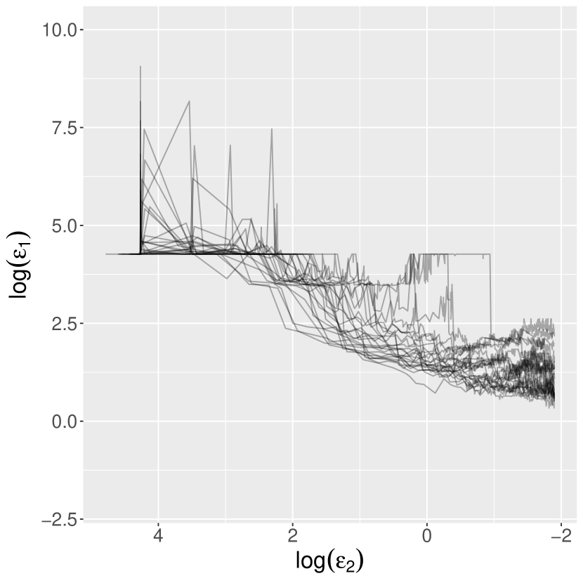
(a) DA-ABC-SMC: $N=500$, $U=100$, $A=100$, $s=0.1$.

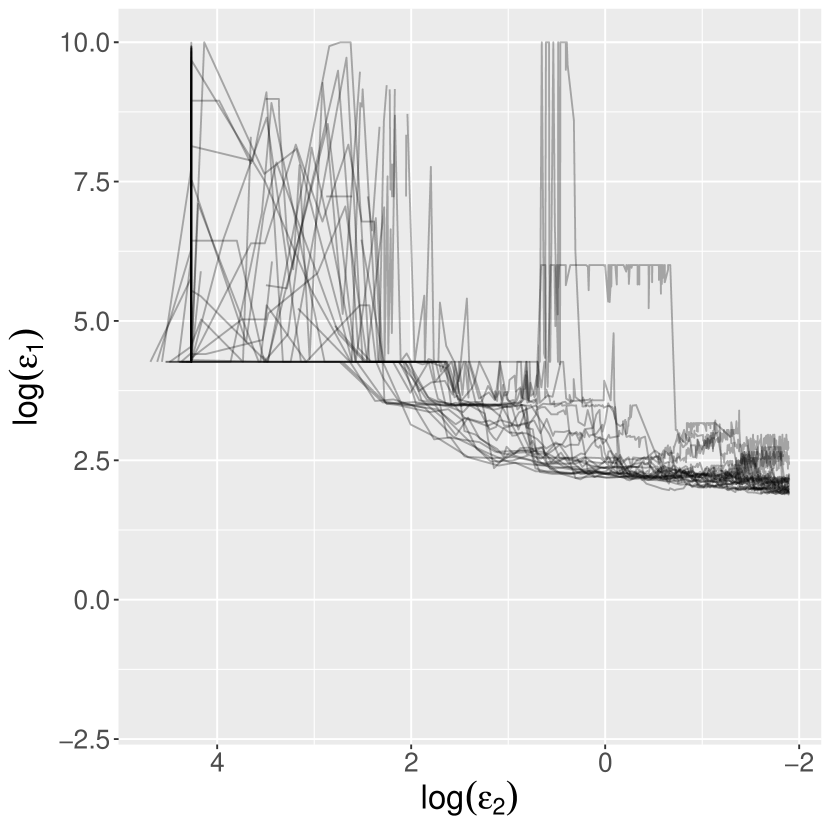
(b) DA-ABC-SMC: $N=500$, $U=100$, $A=100$, $s=0.5$.

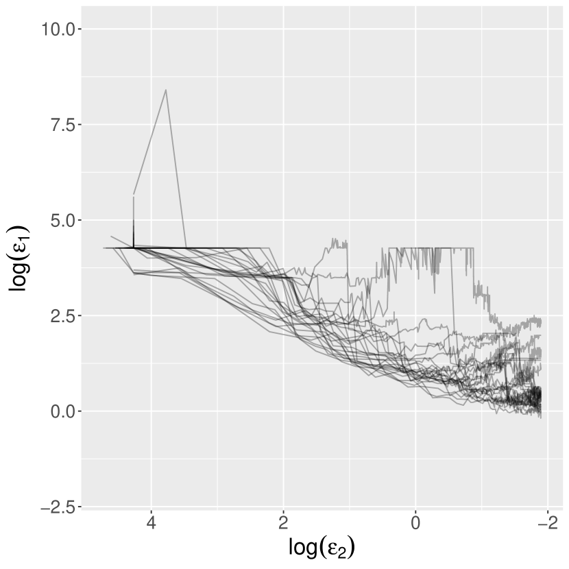
(c) DA-ABC-SMC: $N=1000$, $U=100$, $A=100$, $s=0.1$.

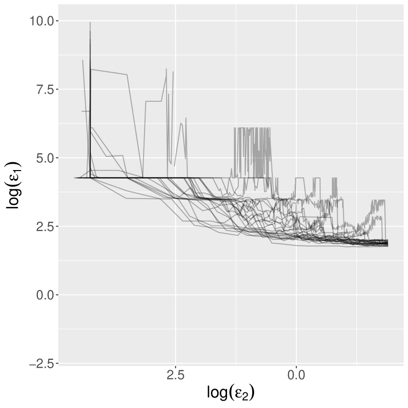
(d) DA-ABC-SMC: $N=1000$, $U=100$, $A=100$, $s=0.5$.

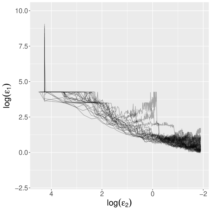
(e) DA-ABC-SMC: $N=1000$, $U=200$, $A=100$, $s=0.1$.

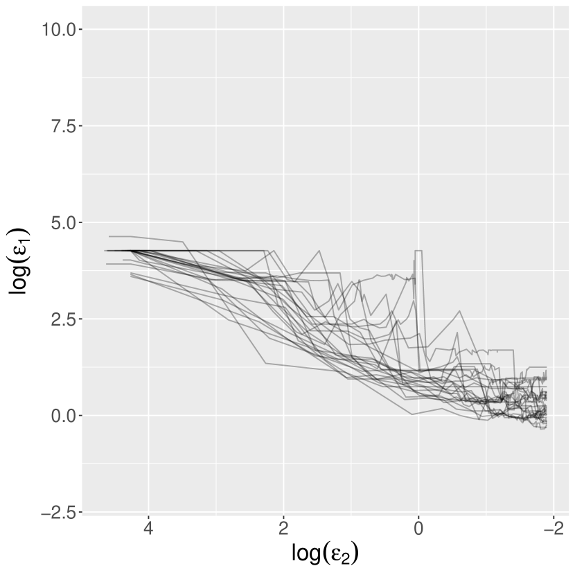
(f) DA-ABC-SMC: $N=1000$, $U=50$, $A=100$, $s=0.1$.

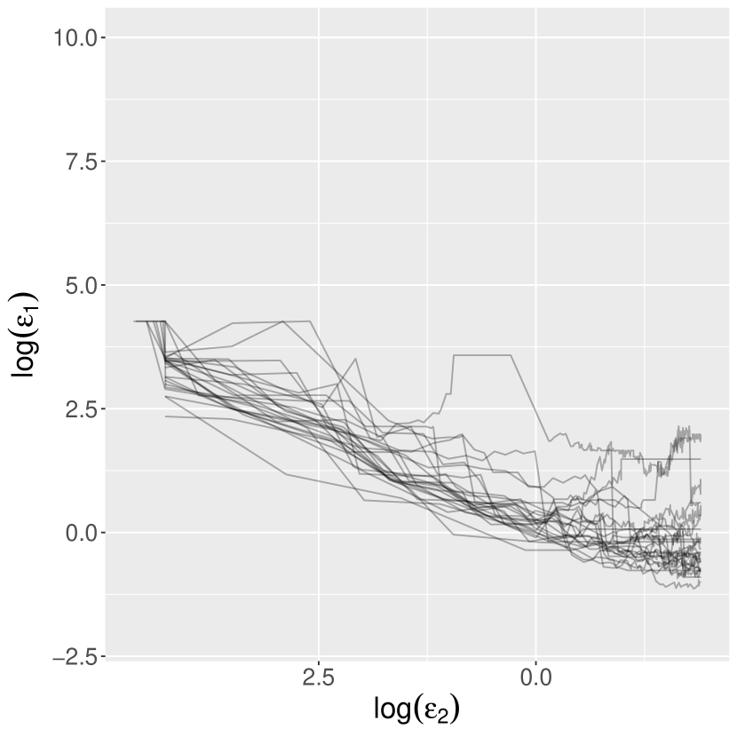
(g) DA-ABC-SMC: $N=5000$, $U=100$, $A=100$, $s=0.1$.

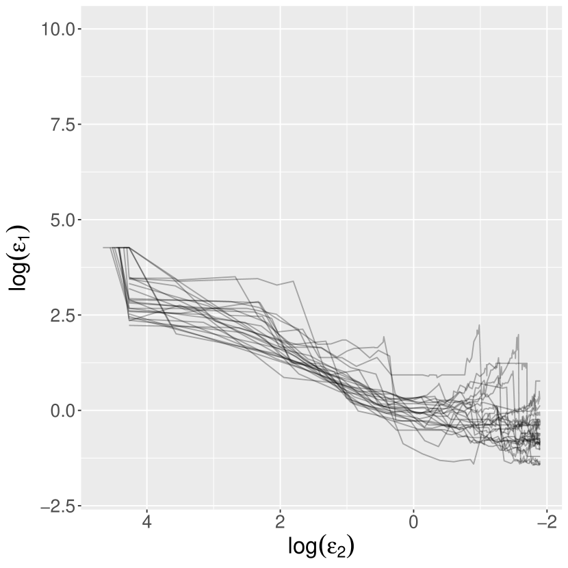
(h) DA-ABC-SMC: $N=10000$, $U=100$, $A=100$, $s=0.1$.

Figure 4: $\log(\epsilon_{1})$, the tolerance in the first stage of DA, plotted against $\log(\epsilon_{2})$, the tolerance in the second stage of DA.

(a) DA-ABC-SMC: $N=500$, $U=100$, $A=100$, $s=0.1$.

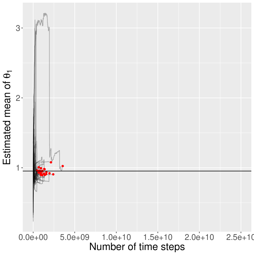
(b) DA-ABC-SMC: $N=500$, $U=100$, $A=100$, $s=0.5$.

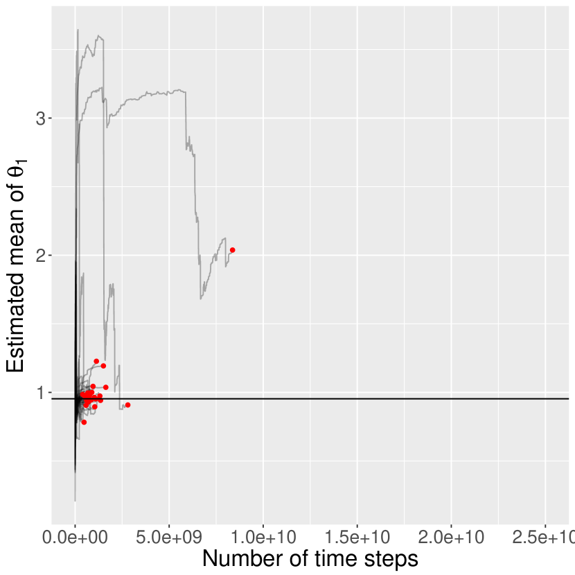
(c) DA-ABC-SMC: $N=1000$, $U=100$, $A=100$, $s=0.1$.

(d) DA-ABC-SMC: $N=1000$, $U=100$, $A=100$, $s=0.5$.

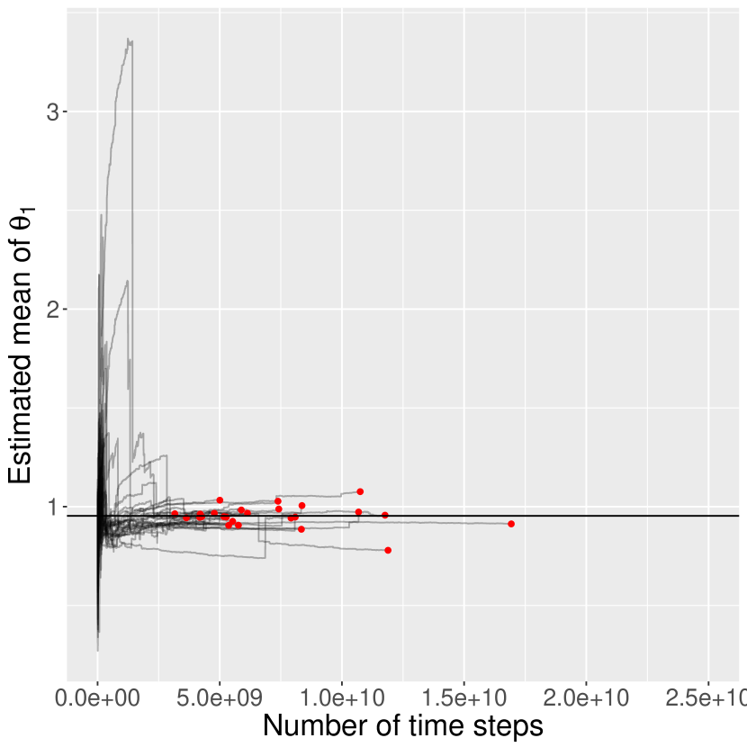
(e) DA-ABC-SMC: $N=1000$, $U=200$, $A=100$, $s=0.1$.

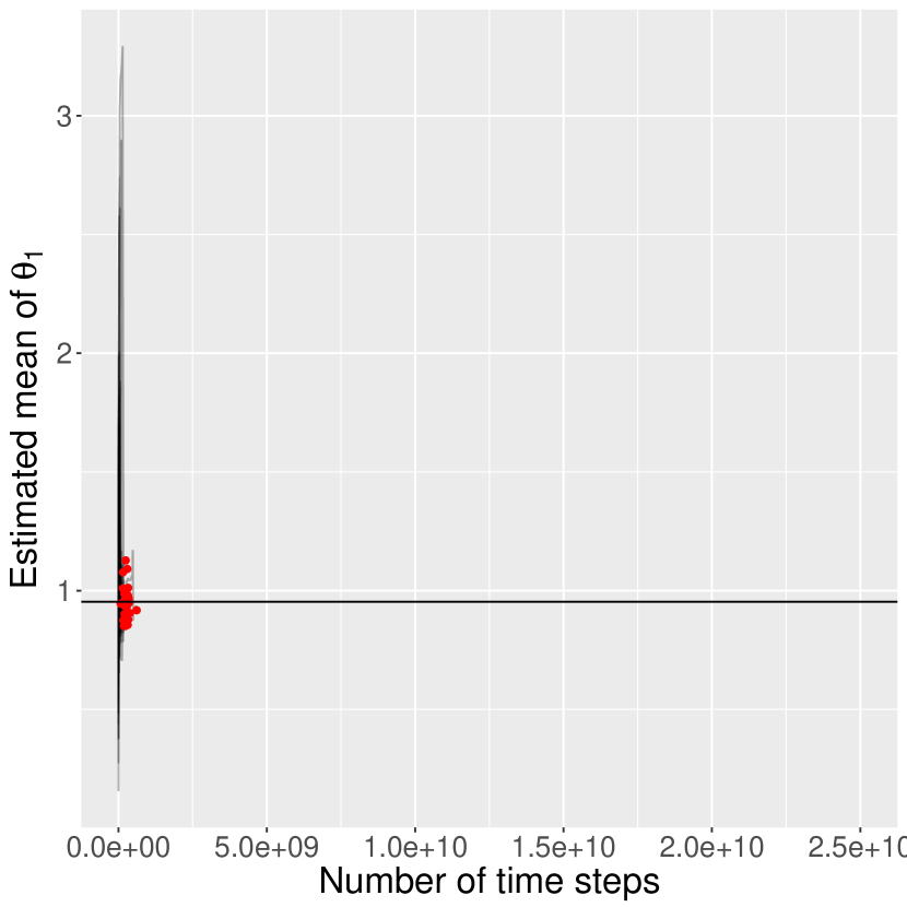
(f) DA-ABC-SMC: $N=1000$, $U=50$, $A=100$, $s=0.1$.

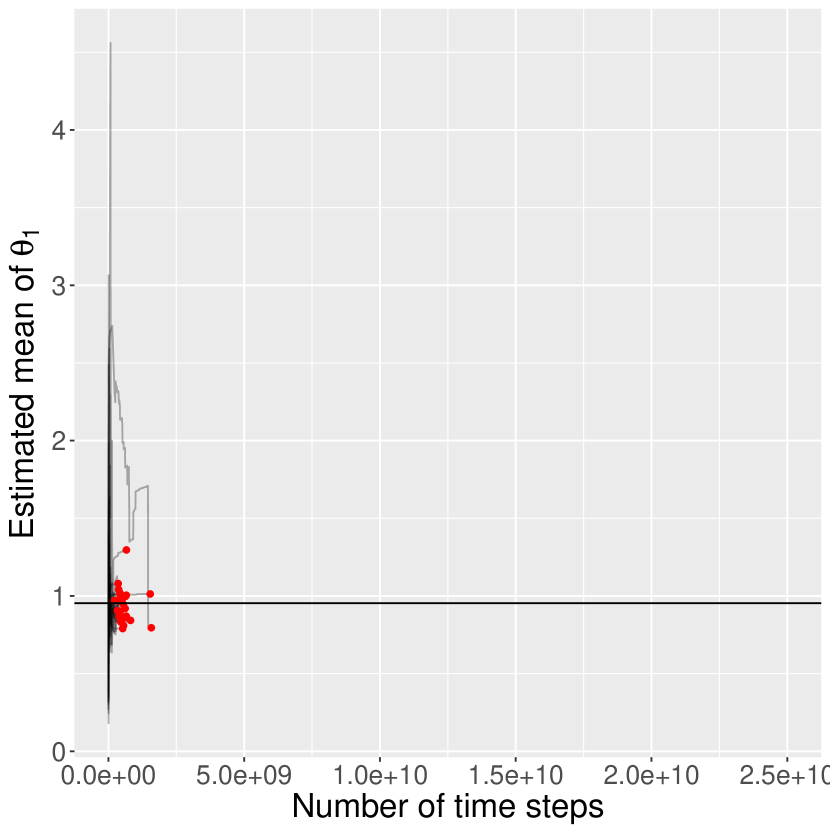
(g) DA-ABC-SMC: $N=5000$, $U=100$, $A=100$, $s=0.1$.

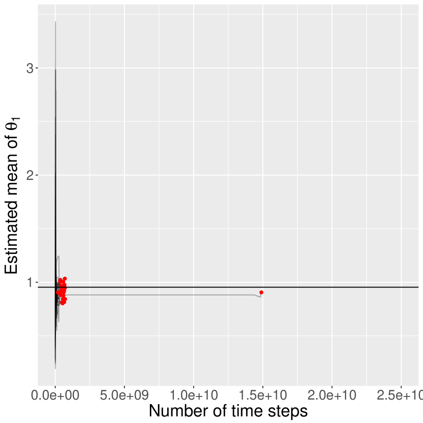
(h) DA-ABC-SMC: $N=10000$, $U=100$, $A=100$, $s=0.1$.

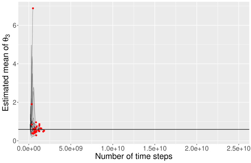
(i) SMC²: $N=100$, $M=100$, $\alpha=0.9$, $s=0.1$.

(j) SMC²: $N=100$, $M=100$, $\alpha=0.99$, $s=0.1$.

(k) SMC²: $N=100$, $M=1000$, $\alpha=0.9$, $s=0.1$.

(l) ABC-SMC: $N=200$, $U=100$.

Figure 5: The estimated posterior mean of $\theta_{1}$ plotted against the total number of time steps used in Euler-Maruyama. Ground truth from ABC-MCMC is marked with a horizontal line.

(a) DA-ABC-SMC: $N=500$, $U=100$, $A=100$, $s=0.1$.

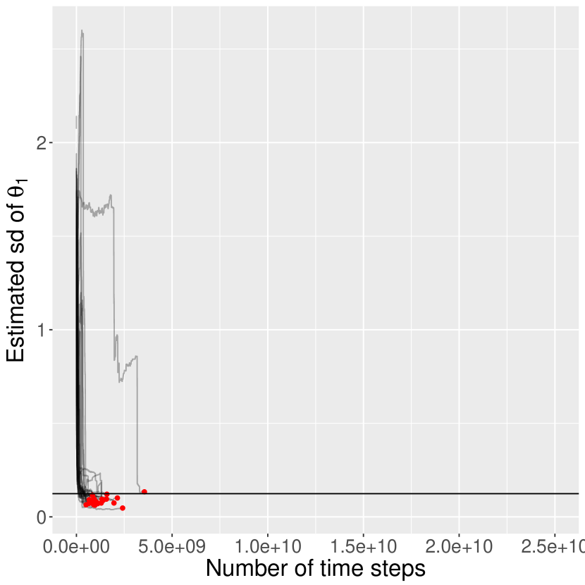
(b) DA-ABC-SMC: $N=500$, $U=100$, $A=100$, $s=0.5$.

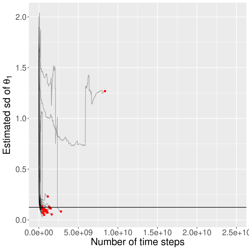
(c) DA-ABC-SMC: $N=1000$, $U=100$, $A=100$, $s=0.1$.

(d) DA-ABC-SMC: $N=1000$, $U=100$, $A=100$, $s=0.5$.

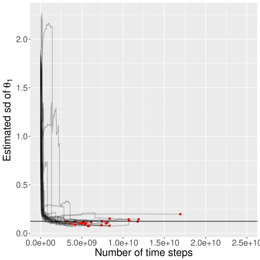
(e) DA-ABC-SMC: $N=1000$, $U=200$, $A=100$, $s=0.1$.

(f) DA-ABC-SMC: $N=1000$, $U=50$, $A=100$, $s=0.1$.

(g) DA-ABC-SMC: $N=5000$, $U=100$, $A=100$, $s=0.1$.

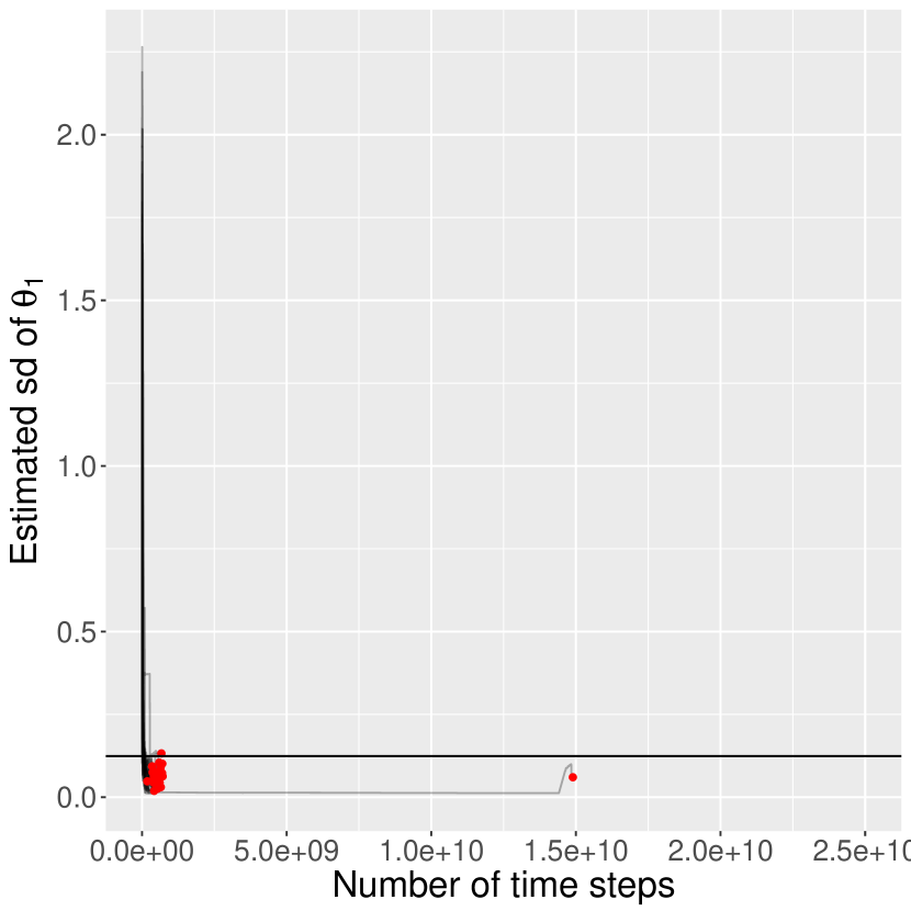
(h) DA-ABC-SMC: $N=10000$, $U=100$, $A=100$, $s=0.1$.

(i) ABC-SMC: $N=200$, $U=100$.

Figure 6: The estimated posterior standard deviation of $\theta_{1}$ plotted against the total number of time steps used in Euler-Maruyama. Ground truth from ABC-MCMC is marked with a horizontal line.

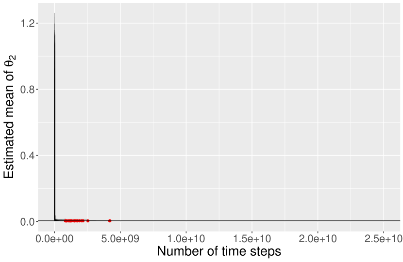
(a) DA-ABC-SMC: $N=500$, $U=100$, $A=100$, $s=0.1$.

(b) DA-ABC-SMC: $N=500$, $U=100$, $A=100$, $s=0.5$.

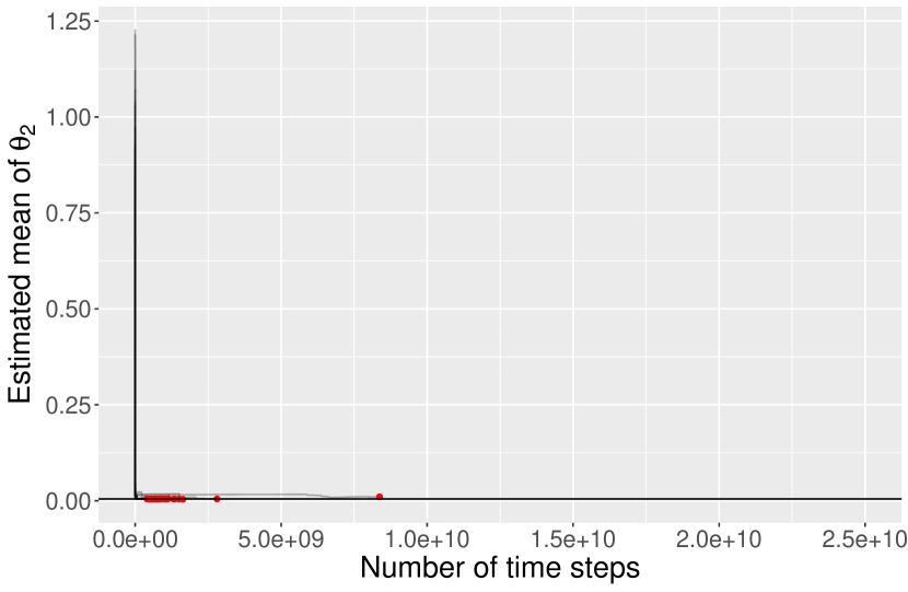
(c) DA-ABC-SMC: $N=1000$, $U=100$, $A=100$, $s=0.1$.

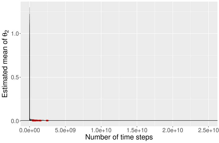
(d) DA-ABC-SMC: $N=1000$, $U=100$, $A=100$, $s=0.5$.

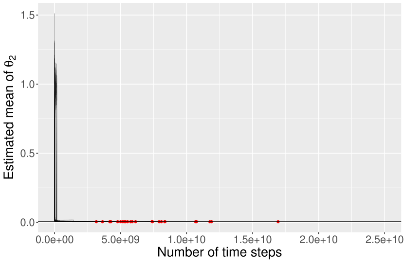
(e) DA-ABC-SMC: $N=1000$, $U=200$, $A=100$, $s=0.1$.

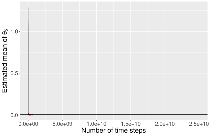
(f) DA-ABC-SMC: $N=1000$, $U=50$, $A=100$, $s=0.1$.

(g) DA-ABC-SMC: $N=5000$, $U=100$, $A=100$, $s=0.1$.

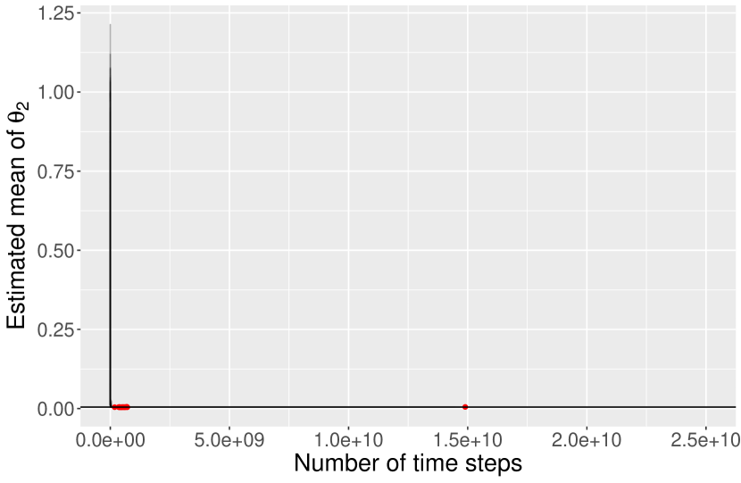
(h) DA-ABC-SMC: $N=10000$, $U=100$, $A=100$, $s=0.1$.

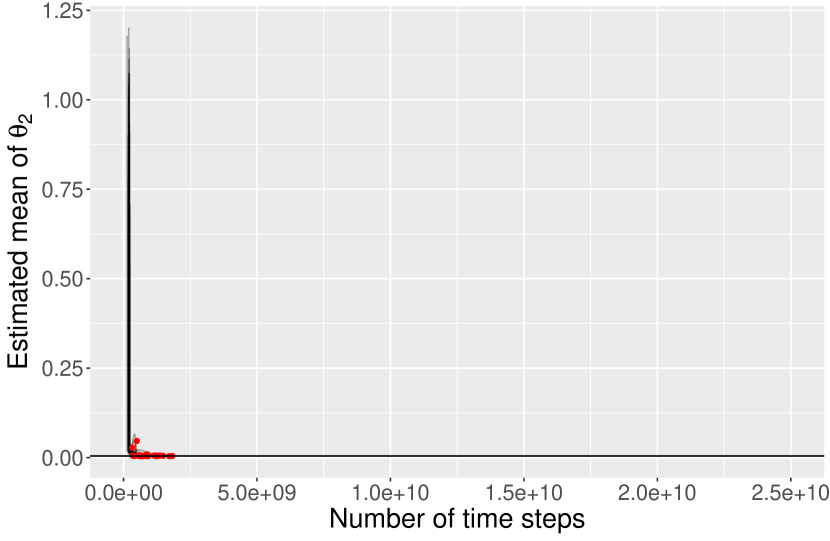
(i) SMC²: $N=100$, $M=100$, $\alpha=0.9$, $s=0.1$.

(j) SMC²: $N=100$, $M=100$, $\alpha=0.99$, $s=0.1$.

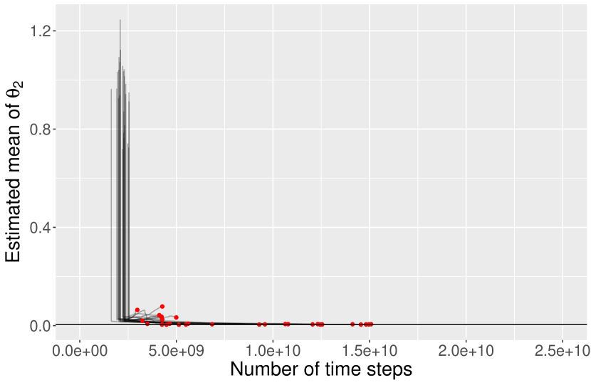
(k) SMC²: $N=100$, $M=1000$, $\alpha=0.9$, $s=0.1$.

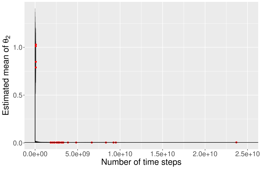
(l) ABC-SMC: $N=200$, $U=100$.

Figure 7: The estimated posterior mean of $\theta_{2}$ plotted against the total number of time steps used in Euler-Maruyama. Ground truth from ABC-MCMC is marked with a horizontal line.

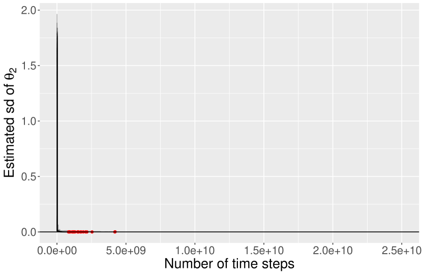
(a) DA-ABC-SMC: $N=500$, $U=100$, $A=100$, $s=0.1$.

(b) DA-ABC-SMC: $N=500$, $U=100$, $A=100$, $s=0.5$.

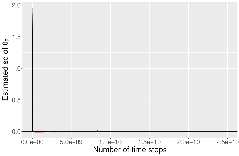
(c) DA-ABC-SMC: $N=1000$, $U=100$, $A=100$, $s=0.1$.

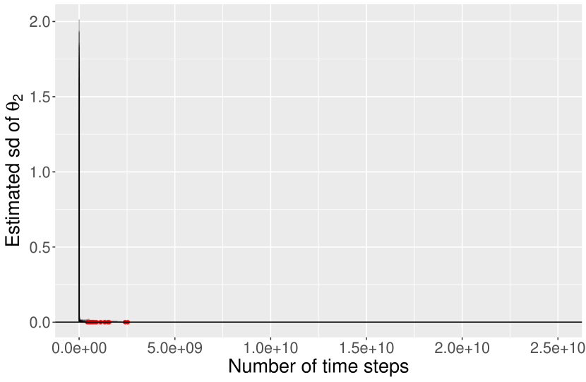
(d) DA-ABC-SMC: $N=1000$, $U=100$, $A=100$, $s=0.5$.

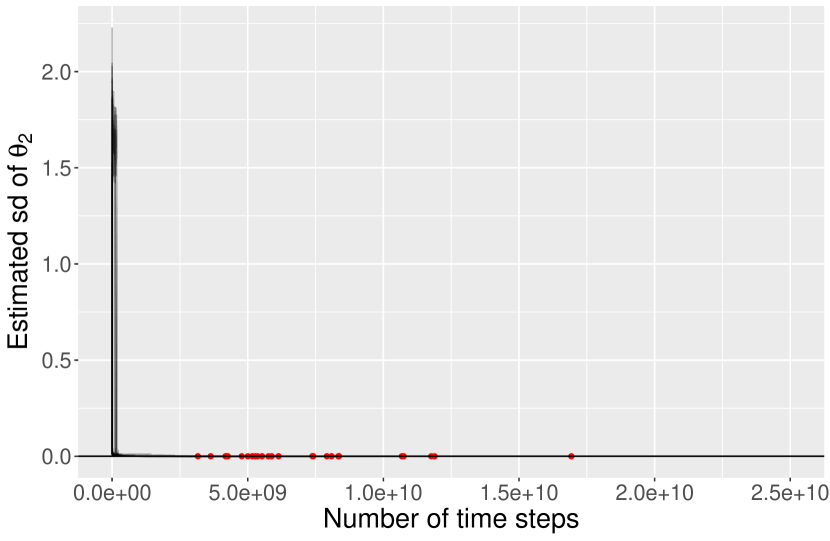
(e) DA-ABC-SMC: $N=1000$, $U=200$, $A=100$, $s=0.1$.

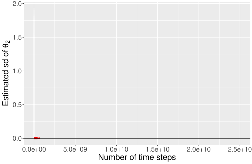
(f) DA-ABC-SMC: $N=1000$, $U=50$, $A=100$, $s=0.1$.

(g) DA-ABC-SMC: $N=5000$, $U=100$, $A=100$, $s=0.1$.

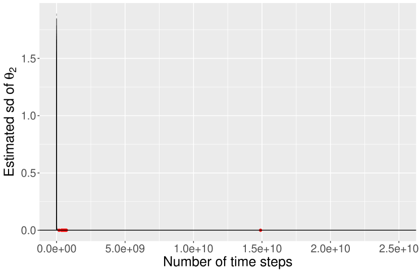
(h) DA-ABC-SMC: $N=10000$, $U=100$, $A=100$, $s=0.1$.

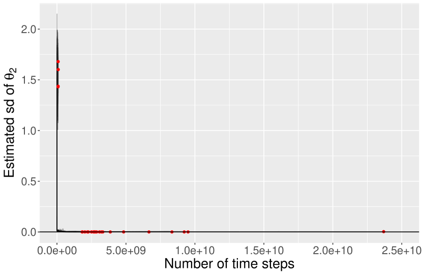
(i) ABC-SMC: $N=200$, $U=100$.

Figure 8: The estimated posterior standard deviation of $\theta_{2}$ plotted against the total number of time steps used in Euler-Maruyama. Ground truth from ABC-MCMC is marked with a horizontal line.

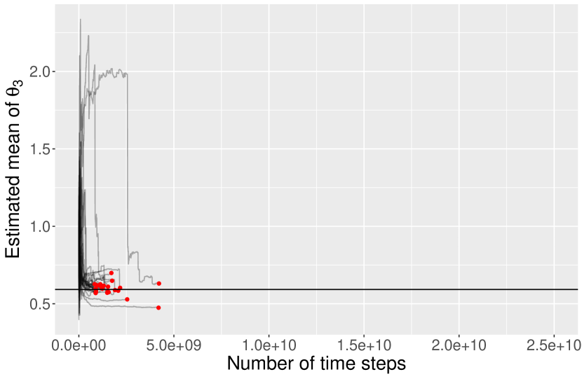
(a) DA-ABC-SMC: $N=500$, $U=100$, $A=100$, $s=0.1$.

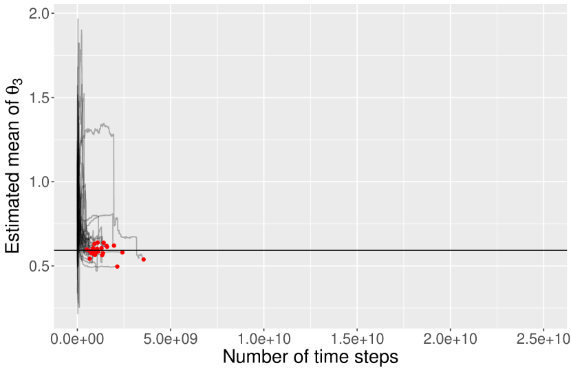
(b) DA-ABC-SMC: $N=500$, $U=100$, $A=100$, $s=0.5$.

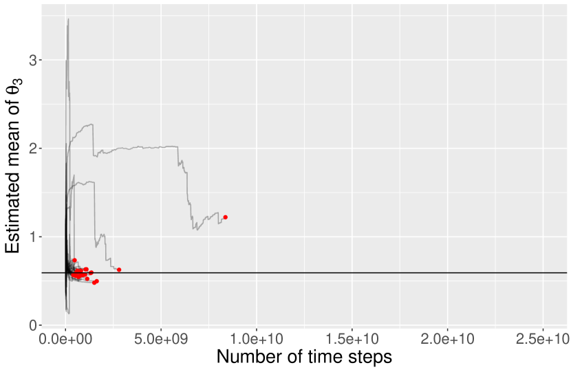
(c) DA-ABC-SMC: $N=1000$, $U=100$, $A=100$, $s=0.1$.

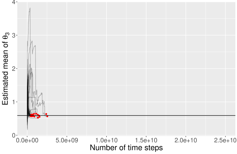
(d) DA-ABC-SMC: $N=1000$, $U=100$, $A=100$, $s=0.5$.

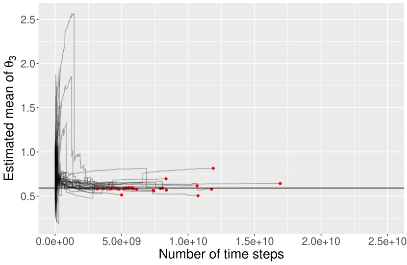
(e) DA-ABC-SMC: $N=1000$, $U=200$, $A=100$, $s=0.1$.

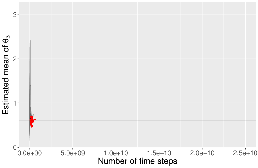
(f) DA-ABC-SMC: $N=1000$, $U=50$, $A=100$, $s=0.1$.

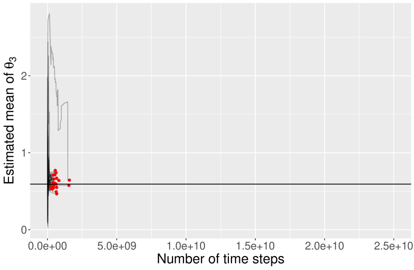
(g) DA-ABC-SMC: $N=5000$, $U=100$, $A=100$, $s=0.1$.

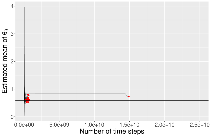
(h) DA-ABC-SMC: $N=10000$, $U=100$, $A=100$, $s=0.1$.

(i) SMC²: $N=100$, $M=100$, $\alpha=0.9$, $s=0.1$.

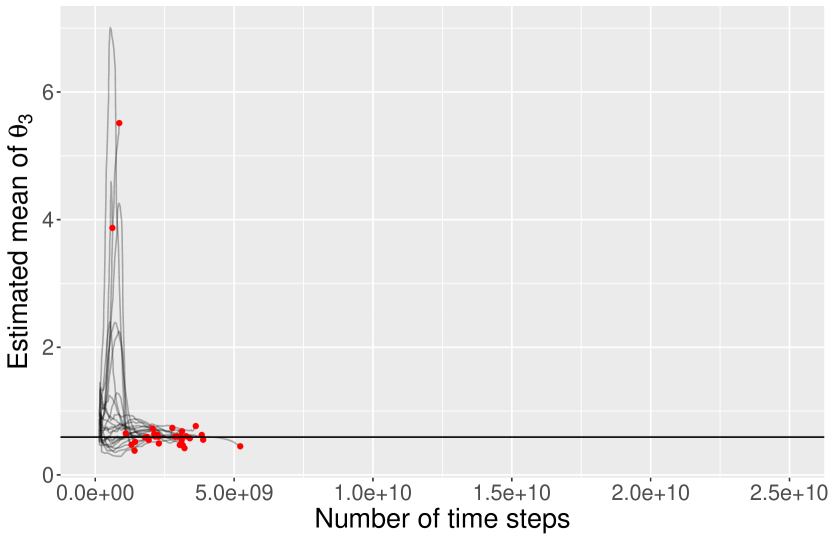
(j) SMC²: $N=100$, $M=100$, $\alpha=0.99$, $s=0.1$.

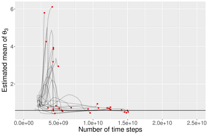
(k) SMC²: $N=100$, $M=1000$, $\alpha=0.9$, $s=0.1$.

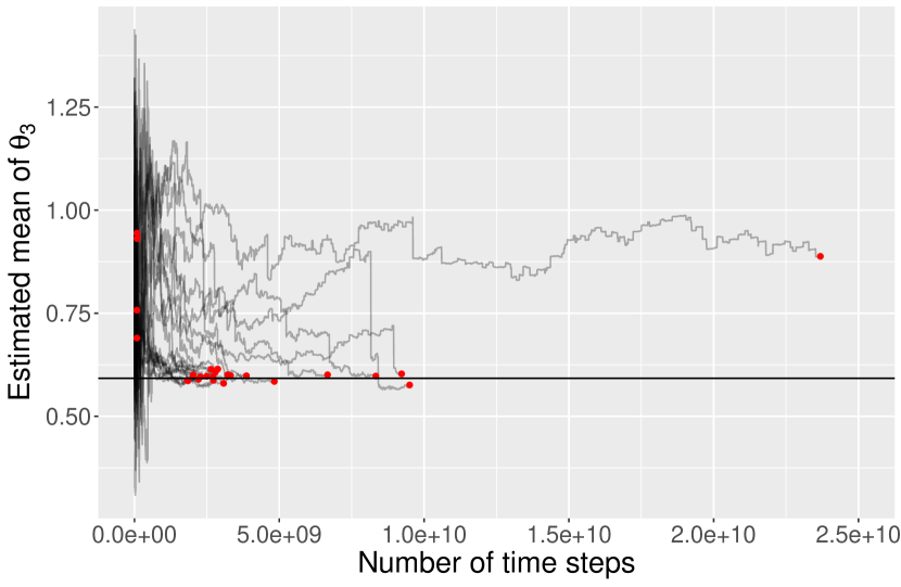
(l) ABC-SMC: $N=200$, $U=100$.

Figure 9: The estimated posterior mean of $\theta_{3}$ plotted against the total number of time steps used in Euler-Maruyama. Ground truth from ABC-MCMC is marked with a horizontal line.

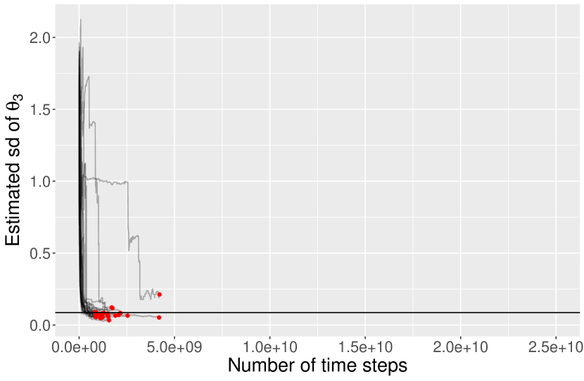
(a) DA-ABC-SMC: $N=500$, $U=100$, $A=100$, $s=0.1$.

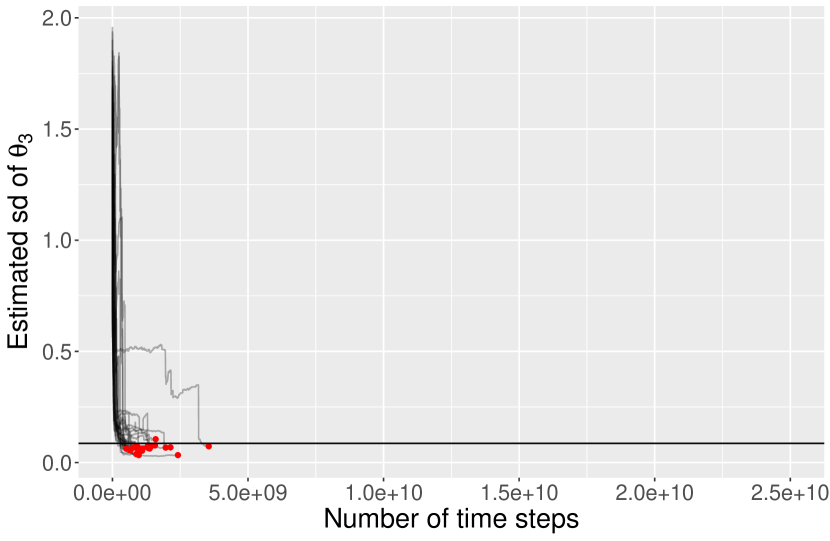
(b) DA-ABC-SMC: $N=500$, $U=100$, $A=100$, $s=0.5$.

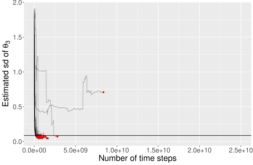
(c) DA-ABC-SMC: $N=1000$, $U=100$, $A=100$, $s=0.1$.

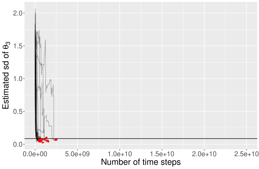
(d) DA-ABC-SMC: $N=1000$, $U=100$, $A=100$, $s=0.5$.

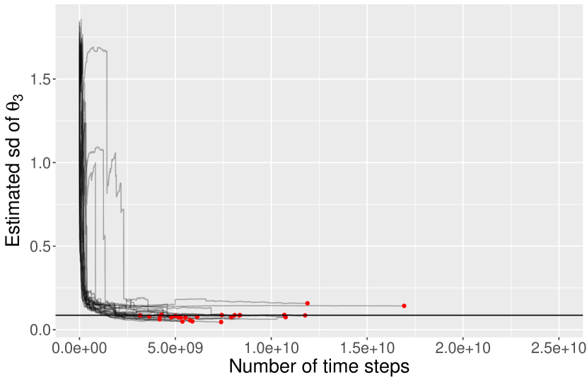
(e) DA-ABC-SMC: $N=1000$, $U=200$, $A=100$, $s=0.1$.

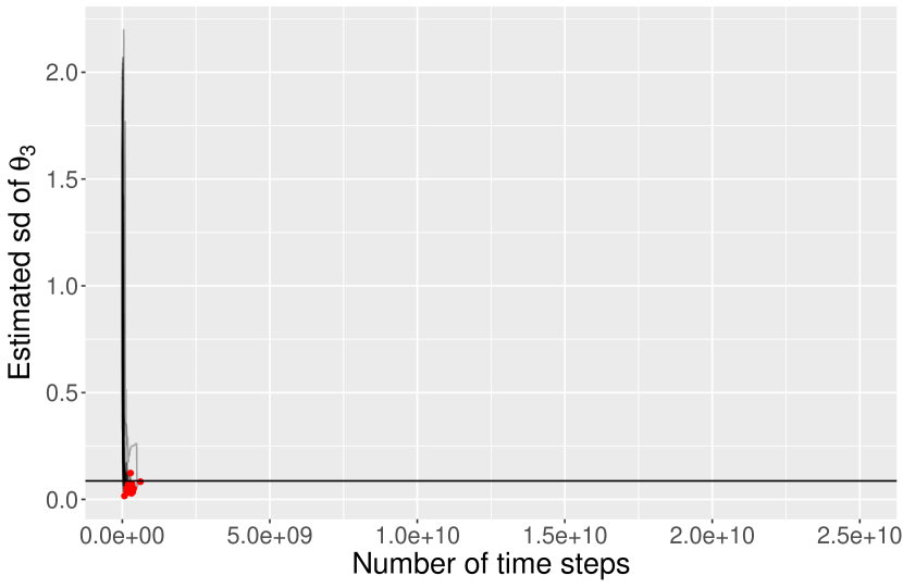
(f) DA-ABC-SMC: $N=1000$, $U=50$, $A=100$, $s=0.1$.

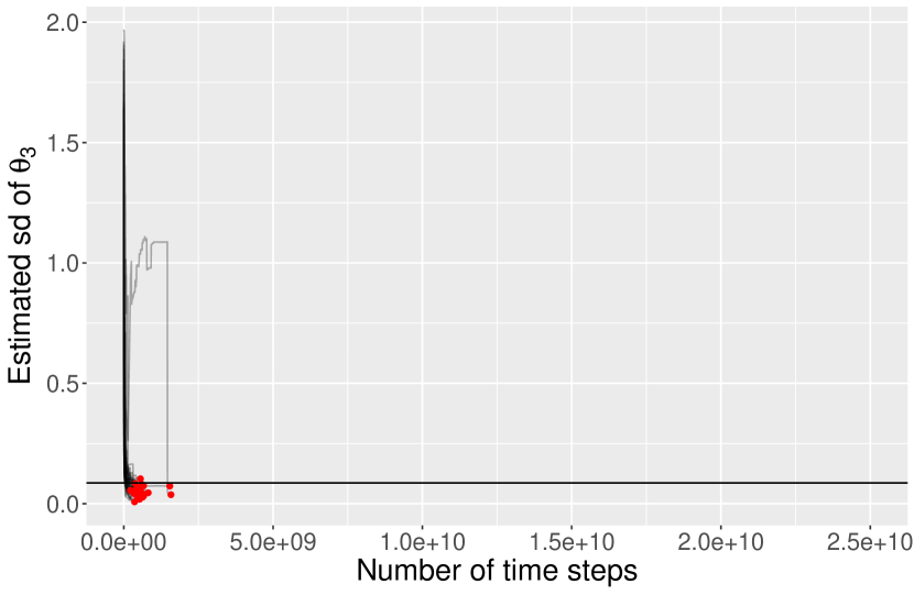
(g) DA-ABC-SMC: $N=5000$, $U=100$, $A=100$, $s=0.1$.

(h) DA-ABC-SMC: $N=10000$, $U=100$, $A=100$, $s=0.1$.

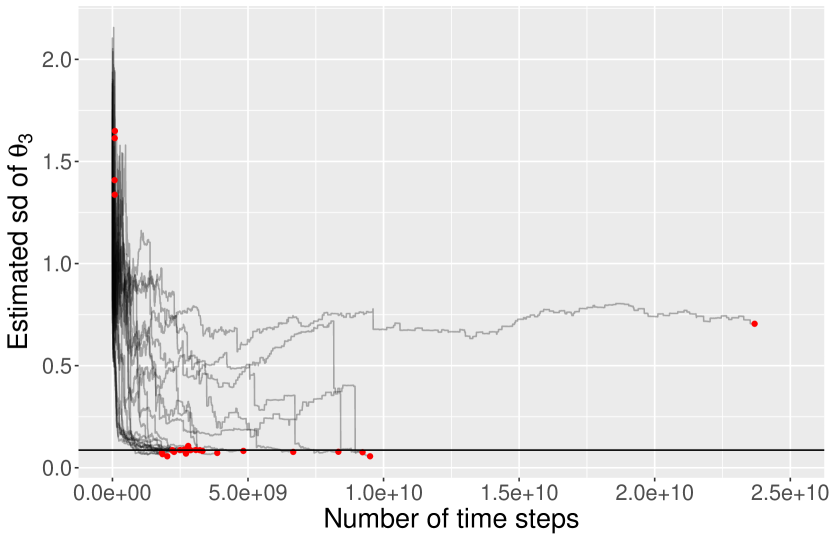
(i) ABC-SMC: $N=200$, $U=100$.

Figure 10: The estimated posterior standard deviation of $\theta_{3}$ plotted against the total number of time steps used in Euler-Maruyama. Ground truth from ABC-MCMC is marked with a horizontal line.

Appendix D Latent exponential random graph model

An exponential random graph model (ERGM) is a model for network data in which the global network structure is modelled as having arisen through local interactions. In this section we consider the situation in which the network is not directly observed, thus $x^{h}$ is a hidden network made up of a random variable for each edge which takes value 1 if the edge is present and 0 if it is absent, and $y$ is a noisy observation of this network. The ERGM on $x^{h}$ is

$$l\left(x^{h}\mid\theta_{x}\right)\propto\exp\left(\theta_{x}^{T}S\left(x^{h}\right)\right),$$

with an intractable normalising constant, and our noisy observations are modelled by

$$g\left(y_{i}\mid x_{i}^{h},\theta_{y}\right)\propto\exp\left(\theta_{y}\left(2x_{i}^{h}-1\right)\left(2y_{i}-1\right)\right)$$

where the normalising constant is tractable. We studied the Dolphin network (figure 11(a)) (Lusseau et al., 2003), as also analysed in Caimo and Friel (2011) where the network is treated as directly observed, and used the same summary statistics and priors as in this paper. The igraph package (Csardi and Nepusz, 2006) was used to load this data into R. We used the statistics

$$S_{1}(x^{h})=\sum_{i<j}x^{h}_{ij}$$ the number of edges

$$S_{2}(x^{h})=\exp\left(\phi_{u}\right)\sum_{i=1}^{n-1}\left\{1-\left(1-\exp\left(-\phi_{u}\right)\right)^{i}\right\}D_{i}\left(x^{h}\right)$$ geometrically weighted degree

$$S_{3}(x^{h})=\exp\left(\phi_{v}\right)\sum_{i=1}^{n-2}\left\{1-\left(1-\exp\left(-\phi_{v}\right)\right)^{i}\right\}EP_{i}\left(x^{h}\right)$$ geometrically weighted edgewise shared partner

with $\phi_{u}=\phi_{v}=0.8$, the prior on $\theta_{x}=(\theta_{1},\theta_{2},\theta_{3})$ and $\theta_{y}$ was $\left(\theta_{1},\theta_{2},\theta_{3},\theta_{y}\right)\sim\mathcal{N}(0,30I_{4})$; and we used the Euclidean distance to compare simulated with observed statistics. The ergm package (Hunter et al., 2008) in R was used to simulate from $l\left(\cdot\mid\theta_{x}\right)$, which uses the “tie no tie” (TNT) sampler and the expensive simulator used $15,000$ iterations. Our DA-ABC-SMC algorithm used $U=A=100$, and again the MCMC proposal was taken to be a Gaussian distribution centred at the current particle, with covariance given by the sample covariance of the particles from the previous iteration.

We ran DA-ABC-SMC for $N=1,000$, and a cheap simulator having $B=1,500$ (after exploratory runs suggested that this would be enough iterations to provide a useful DA proposal) and compared the results with standard ABC-SMC with the same configuration as in the previous section (both using $3\times 10^{8}$ iterations of the TNT sampler). Figure 11(b) shows the results from the two algorithms, this time showing the sequence $\epsilon_{1,t}$ alongside the sequence $\epsilon_{2,t}$. Again we observe that the tolerance in DA-ABC-SMC reduces faster than standard ABC-SMC, and that the tolerance $\epsilon_{1,t}$ changes adaptively. This data has not previously been studied using a latent ERGM. Using particle MCMC as in Everitt (2012) would require at every MCMC iteration to run an SMC sampler to integrate out the latent ERGM space, which consists of 1891 binary edge variables. We might expect that many SMC particles would be required to produce low variance marginal likelihood estimates, leading to a high computational cost. However, the acceptance rate was very low towards the end of our ABC runs, suggesting that a very large computational cost would be required to reduce $\epsilon_{2,t}$ to be close to zero.

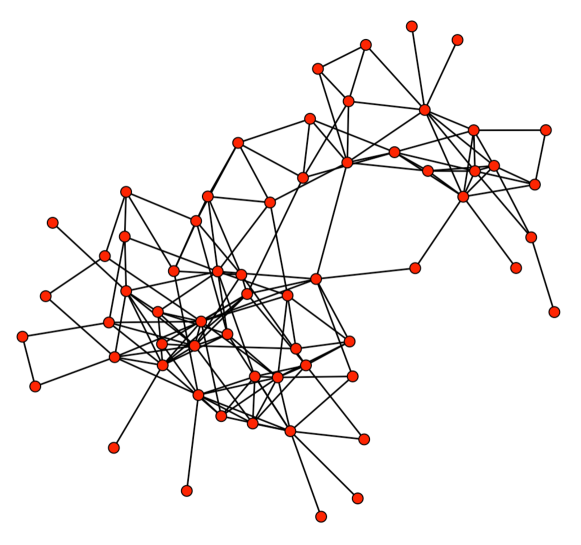
(a) The Dolphin network.

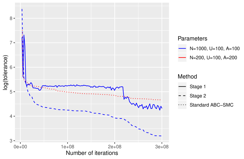
(b) ABC tolerance plotted against the number of iterations of the TNT sampler.

Figure 11: DA-ABC-SMC applied to the latent ERGM.

References

- Andrieu and Roberts (2009) Andrieu, C. and Roberts, G. O. (2009, apr). The pseudo-marginal approach for efficient Monte Carlo computations. The Annals of Statistics 37(2), 697–725.
- Banterle et al. (2014) Banterle, M., Grazian, C., and Robert, C. P. (2014). Accelerating Metropolis-Hastings algorithms: Delayed acceptance with prefetching. arXiv (arXiv:1406.2660).
- Beaumont et al. (2002) Beaumont, M. A., Zhang, W., and Balding, D. J. (2002, dec). Approximate Bayesian computation in population genetics. Genetics 162(4), 2025–35.
- Bernton et al. (2017) Bernton, E., Jacob, P. E., Gerber, M., and Robert, C. P. (2017). Inference in generative models using the Wasserstein distance. arXiv (arXiv:1701.05146).
- Caimo and Friel (2011) Caimo, A. and Friel, N. (2011). Bayesian inference for exponential random graph models. Social Networks, 33, 41–55.
- Cérou et al. (2012) Cérou, F., Del Moral, P., Furon, T., and Guyader, A. (2012). Sequential Monte Carlo for rare event estimation. Statistics and Computing 22(3), 795–908.
- Chopin et al. (2013) Chopin, N., Jacob, P. E., and Papaspiliopoulos, O. (2013). SMC2: an efficient algorithm for sequential analysis of state space models. Journal of the Royal Statistical Society: Series B 75(3), 397–426.
- Christen and Fox (2005) Christen, J. A. and Fox, C. (2005, dec). Markov chain Monte Carlo Using an Approximation. Journal of Computational and Graphical Statistics 14(4), 795–810.
- Csardi and Nepusz (2006) Csardi, G. and Nepusz, T. (2006). The igraph software package for complex network research. InterJournal, Complex Systems, 1695.
- Del Moral et al. (2006) Del Moral, P., Doucet, A., and Jasra, A. (2006). Sequential Monte Carlo samplers. Journal of the Royal Statistical Society: Series B 68(3), 411–436.
- Del Moral et al. (2012a) Del Moral, P., Doucet, A., and Jasra, A. (2012a). An adaptive sequential Monte Carlo method for approximate Bayesian computation. Statistics and Computing 22(5), 1009–1020.
- Del Moral et al. (2012b) Del Moral, P., Doucet, A., and Jasra, A. (2012b). On adaptive resampling strategies fo sequential Monte Carlo methods. Bernoulli 18(1).
- Del Moral et al. (2015) Del Moral, P., Jasra, A., Lee, A., Yau, C., and Zhang, X. (2015). The Alive Particle Filter and Its Use in Particle Markov Chain Monte Carlo. Stochastic Analysis and Applications 33(6), 943–974.
- Didelot et al. (2011) Didelot, X., Everitt, R. G., Johansen, A. M., and Lawson, D. J. (2011). Likelihood-free estimation of model evidence. Bayesian Analysis 6(1), 49–76.
- Duan and Fulop (2015) Duan, J. C. and Fulop, A. (2015). Density-Tempered Marginalized Sequential Monte Carlo Samplers. Journal of Business and Economic Statistics 33(2), 192–202.
- Everitt (2012) Everitt, R. G. (2012). Bayesian Parameter Estimation for Latent Markov Random Fields and Social Networks. Journal of Computational and Graphical Statistics 21(4), 940–960.
- Everitt et al. (2017) Everitt, R. G., Johansen, A. M., Rowing, E., and Evdemon-Hogan, M. (2017). Bayesian model comparison with un-normalised likelihoods. Statistics and Computing 27(2), 403–422.
- Everitt et al. (2017) Everitt, R. G., Prangle, D., Maybank, P., and Bell, M. (2017). Marginal sequential Monte Carlo for doubly intractable models. arXiv (arXiv:1710.04382).
- Friel (2013) Friel, N. (2013). Evidence and Bayes factor estimation for Gibbs random fields. Journal of Computational and Graphical Statistics 22(3), 518–532.
- Genz and Bretz (2009) Genz, A. and Bretz, F. (2009). Computation of Multivariate Normal and t Probabilities. Lecture Notes in Statistics. Heidelberg: Springer-Verlag.
- Gillespie (1977) Gillespie, D. T. (1977). Exact stochastic simulation of coupled chemical reactions. Journal of Physical Chemistry 8(25), 2340–2361.
- Golightly et al. (2015) Golightly, A., Henderson, D. A., and Sherlock, C. (2015). Delayed acceptance particle MCMC for exact inference in stochastic biochemical network models. Statistics and Computing 25(5), 1039–1055.
- Grelaud et al. (2009) Grelaud, A., Robert, C. P., and Marin, J.-M. (2009). ABC likelihood-free methods for model choice in Gibbs random fields. Bayesian Analysis 4(2), 317–336.
- Hunter et al. (2008) Hunter, D. R., Handcock, M. S., Butts, C. T., Goodreau, S. M., and Morris, M. (2008). ergm: A package to fit, simulate and diagnose exponential-family models for networks. Journal of Statistical Software 24(3), 1–29.
- Kong et al. (1994) Kong, A., Liu, J. S., and Wong, W. H. (1994). Sequential Imputations and Bayesian Missing Data Problems. Journal of the American Statistical Association 89(425), 278–288.
- Li and Fearnhead (2018) Li, W. and Fearnhead, P. (2018). On the asymptotic efficiency of approximate bayesian computation estimators. Biometrika 105(2), 285–299.
- Lusseau et al. (2003) Lusseau, D., Schneider, K., Boisseau, O. J., Haase, P., Slooten, E., and Dawson, S. M. (2003, sep). The bottlenose dolphin community of Doubtful Sound features a large proportion of long-lasting associations. Behavioral Ecology and Sociobiology 54(4), 396–405.
- Marjoram et al. (2003) Marjoram, P., Molitor, J., Plagnol, V., and Tavare, S. (2003). Markov chain monte carlo without likelihoods. Proceedings of the National Academy of Sciences of the United States of America 100(26), 15324–15328.
- Møller et al. (2006) Møller, J., Pettitt, A. N., Reeves, R. W., and Berthelsen, K. K. (2006, jun). An efficient Markov chain Monte Carlo method for distributions with intractable normalising constants. Biometrika 93(2), 451–458.
- Murray et al. (2006) Murray, I., Ghahramani, Z., and MacKay, D. J. C. (2006). MCMC for doubly-intractable distributions. In Proceedings of the 22nd Annual Conference on Uncertainty in Artificial Intelligence (UAI), pp. 359–366.
- Papamakarios and Murray (2016) Papamakarios, G. and Murray, I. (2016). Fast Epsilon-Free Inference of Simulation Models with Bayesian Conditional Density Estimation. arXiv (arXiv:1605.06376).
- Picchini (2014) Picchini, U. (2014, apr). Inference for SDE models via Approximate Bayesian Computation. Journal of Computational and Graphical Statistics 23(4), 1080–1100.
- Picchini and Forman (2016) Picchini, U. and Forman, J. L. (2016). Accelerating inference for diffusions observed with measurement error and large sample sizes using Approximate Bayesian Computation: A case study. Journal of Statistical Computation and Simulation 86(1), 195–213.
- Prangle (2016) Prangle, D. (2016). Lazy ABC. Statistics and Computing 26(1-2), 171–185.
- Prangle et al. (2017) Prangle, D., Everitt, R. G., and Kypraios, T. (2017). A rare event approach to high dimensional approximate Bayesian computation. Statistics and Computing 28(4), 819–834.
- Pritchard et al. (1999) Pritchard, J. K., Seielstad, M. T., Perez-Lezaun, A., and Feldman, M. W. (1999, dec). Population growth of human Y chromosomes: a study of Y chromosome microsatellites. Molecular Biology and Evolution 16(12), 1791–8.
- R Core Team (2019) R Core Team (2019). R: A Language and Environment for Statistical Computing. Vienna, Austria: R Foundation for Statistical Computing.
- Robert et al. (2011) Robert, C. P., Beaumont, M. A., Marin, J.-M., and Cornuet, J.-M. (2011). Adaptivity for ABC algorithms: the ABC-PMC scheme. Biometrika 96(4), 983–990.
- Roebuck (2014) Roebuck, P. (2014). matlab: MATLAB emulation package. R package version 1.0.2.
- Sherlock et al. (2017) Sherlock, C., Golightly, A., and Henderson, D. A. (2017). Adaptive, delayed-acceptance MCMC for targets with expensive likelihoods. Journal of Computational and Graphical Statistics 26(2), 434–444.
- Sisson et al. (2007) Sisson, S. A., Fan, Y., and Tanaka, M. M. (2007, feb). Sequential Monte Carlo without likelihoods. Proceedings of the National Academy of Sciences of the United States of America 104(6), 1760–1765.
- Sisson et al. (2009) Sisson, S. A., Fan, Y., and Tanaka, M. M. (2009). Correction: Sequential Monte Carlo without likelihoods. Proceedings of the National Academy of Sciences of the United States of America 106(39), 16889–16890.
- Stoehr (2017) Stoehr, J. (2017). A review on statistical inference methods for discrete Markov random fields. arXiv (arXiv:1704.03331).
- Strens (2004) Strens, M. (2004). Efficient hierarchical MCMC for policy search. Proceedings of the 21st International Conference on Machine Learning, 97.
- Tierney (1998) Tierney, L. (1998). A Note On Metropolis-Hastings Kernels For General State Spaces. Annals of Applied Probability 8(1), 1–9.
- van der Vaart et al. (2015) van der Vaart, E., Beaumont, M. A., Johnston, A. S. A., and Sibly, R. M. (2015). Calibration and evaluation of individual-based models using Approximate Bayesian Computation. Ecological Modelling, 312, 182–190.
- Wickham (2016) Wickham, H. (2016). ggplot2: Elegant Graphics for Data Analysis. Springer-Verlag New York.
- Wilkinson (2018) Wilkinson, D. (2018). smfsb: Stochastic Modelling for Systems Biology. R package version 1.3.
- Wilkinson (2011) Wilkinson, D. J. (2011). Stochastic Modelling for Systems Biology (Second ed.). Boca Raton, Florida: Chapman & Hall/CRC Press.
- Zhou et al. (2016) Zhou, Y., Johansen, A. M., and Aston, J. A. D. (2016). Towards automatic model comparison: an adaptive sequential Monte Carlo approach. Journal of Computational and Graphical Statistics 25(3), 701–726.