Training Deep Networks to be Spatially Sensitive

Abstract

In many computer vision tasks, for example saliency prediction or semantic segmentation, the desired output is a foreground map that predicts pixels where some criteria is satisfied. Despite the inherently spatial nature of this task commonly used learning objectives do not incorporate the spatial relationships between misclassified pixels and the underlying ground truth. The Weighted F-measure, a recently proposed evaluation metric, does reweight errors spatially, and has been shown to closely correlate with human evaluation of quality, and stably rank predictions with respect to noisy ground truths (such as a sloppy human annotator might generate). However it suffers from computational complexity which makes it intractable as an optimization objective for gradient descent, which must be evaluated thousands or millions of times while learning a model’s parameters. We propose a differentiable and efficient approximation of this metric. By incorporating spatial information into the objective we can use a simpler model than competing methods without sacrificing accuracy, resulting in faster inference speeds and alleviating the need for pre/post-processing. We match (or improve) performance on several tasks compared to prior state of the art by traditional metrics, and in many cases significantly improve performance by the weighted F-measure.

1 Introduction

When optimizing a predictive model it is important that the objective function not only encode the ideal solution (zero mistakes), but also quantify the relative severity of mistakes. A common dimension of preference is the desired tradeoff between precision and recall. One can capture this tradeoff with a $F_{\beta}$ metric, where $\beta$ reflects the relative importance of recall compared to precision. While this metric can quantify the relative importance of false positives and false negatives, it cannot capture differing severity between two false positives, or two false negatives. One domain where differentiating between such errors becomes important is the prediction of foreground maps, where the output has many desired properties not captured by notions of precision or recall, such as smoothness, accuracy of boundaries, contiguity of the predicted mask, etc. As a result, two predictions with the same number of mistakes, or with the same score on a measure which treats false positives and false negatives equally (e.g. intersection over union, IoU), may differ substantially in their perceived spatial quality. Loss functions derived from per-pixel classification-based surrogates, such as log-loss are almost universally used in existing work, but fail to capture both the precision-recall tradeoff and the spatial sensibilities of this kind.

[16]	$SZN_{CE}$	$SZN_{F^{w}_{1}}$	GT	Input
	(ours)	(ours)

Figure 1: A comparison of the previous saliency prediction state of the art with our $SZN$ model predictions with the traditional log-loss ($SZN_{CE}$) and our proposed $AF^{w}_{\beta}$ loss ($SZN_{F^{w}_{1}}$). The top row demonstrates that our loss heavily penalizes for large spatially co-occurring false negatives. The bottom row demonstrates that the proposed loss heavily penalizes false positives far from the true object boundary.

Margolin et al. [22] proposed a method to quantify these distinctions when predicting foreground maps. Their $F_{\beta}^{w}$ measure formalizes two notions. First, false detections are less severe when close to the object’s true boundary; Second, missing an entire section of an object is worse than missing the same number of pixels scattered across the entire object. These alterations closely match human intuition and perceptual judgements, and have the additional benefits of being robust to small annotation errors (such as minor differences between multiple human annotators). The $F_{\beta}^{w}$ measure is also able to reliably rank generic foreground maps, such as centered geometric shapes, lower than state of the art predictions (They show traditional metrics, such as AUC, lack this property). Despite these positive traits, their formulation has $O(n^{2})$ memory and computational requirements where $n$ the number of pixels in the image.

This computational cost poses a particular problem if the $F_{\beta}^{w}$ metric were used as the training objective for deep neural networks (DNNs). Normally trained with stochastic gradient descent over large training sets, DNNs require computing the gradient of the loss many, many, times. This means that the loss function must be differentiable, and efficient – two criteria which $F_{\beta}^{w}$ does not meet.

Our primary contribution is a differentiable and computationally efficient approximation of the $F_{\beta}^{w}$ metric, which can be used directly as the loss function of a convolutional neural network (CNN). As a secondary contribution, we propose a memory-efficient CNN architecture which is capable of producing high resolution pixel-wise predictions, taking full advantage of the spatial information provided by our proposed loss. By combining these two components we are able to produce high-fidelity, spatially cohesive predictions, without relying on complex, often expensive pre-processing (such as super-pixels) or post-processing (such as CRF inference), resulting in inference speeds an order of magnitude faster than state of the art in multiple domains. We do not sacrifice accuracy, achieving competitive or state of the art accuracy on benchmarks for salient object detection, portrait segmentation, and visual distractor masking.

2 Background

In this section we discuss the prior work on incorporating spatial consideration into learning objectives. While multiple objectives have been proposed to capture spatial properties of prediction maps [2, 24, 25], these have been limited to structured prediction methods using random fields, and adds significant complexity when incorporated into a feed-forward prediction framework like that of CNNs. We focus on the $F_{\beta}^{w}$ metric, which is decoupled from the prediction framework and upon which we directly build our approach. We review it below, and also survey the related work on the segmentation tasks on which we evaluate our contributions: salient object detection, distractor detection, and portrait segmentation.

2.1 The $F_{\beta}$ metric family

In a binary classification scenario, with labels $y\in\{0,1\}$, when the predicted label $\widehat{y}$ is a mistake $\widehat{y}\neq y$, it is either a false positive (FP, $\widehat{y}=1$) or a false negative (FN, $\widehat{y}=0$). Performance of any classifier on an evaluation set can be characterized by its precision $\#TP/(\#TP+\#FP)$ and its recall $\#TP/(\#TP+\#FN)$.

While precision and recall each only tell part of the story, one can summarize a classification algorithm’s performance in a single number, using the $F_{\beta}$ metric

$$F_{\beta}=\frac{(1+\beta^{2})*Precision*Recall}{\beta^{2}Precision+Recall}.$$ (1)

$\beta$ captures the relative importance of precision compared to recall (e.g. if precision is twice as important as recall, we use $F_{2}$). The well known $F_{1}$ metric is a special case corresponding to equal importance between precision and recall. The $F_{\beta}$ metrics is a common benchmark in ’information extraction’ tasks, and in  [10] Jansche outlines a procedure to directly optimize it. This formulation applies to any scenario when $F_{\beta}$ is meaningful, but it cannot encode differences within the categories of false positive, and false negative, which are quite meaningful in the highly structured domain of natural images.

2.2 The $F_{\beta}^{w}$ metric

The standard $F_{\beta}$ is extended in [22] in two ways. First, it is generalized to handle continuous predictions, $\widehat{y}\in[0,1]$ (the ground truth $y$ remains binary). The adjusted definitions of the true positive, false positive, true negative, and false negative are as follows:

$$\begin{split}E&=|Y-\widehat{Y}|\\ TP&=(1-E)\cdot Y\\ TN&=(1-E)\cdot(1-Y)\\ FP&=E\cdot(1-Y)\\ FN&=E\cdot Y\\ \end{split}$$ (2)

This holds in the case of predicting a set of values; $Y$ is the vector of ground truth labels , $\widehat{Y}$ is the vector of predictions, and $\cdot$ denotes the dot product

The second modification proposed in [22] addresses the unequal nature of mistakes in binary segmentation ($y=1$ implying foreground, $y=0$ background), as determined by the spatial configuration of predictions vs. ground truth. The authors of [22] suggest a number of criteria for evaluating foreground maps.

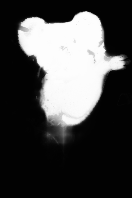
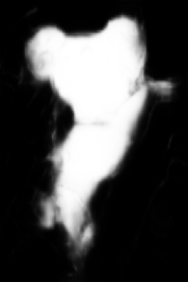
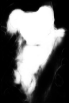
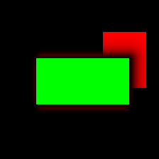
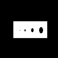
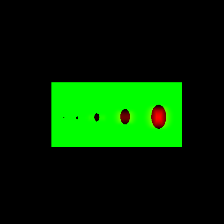
First consider false negatives, missed detections of foreground pixels. If random foreground pixels across an object are undetected, leaving small holes in the foreground, this is easily corrected via post-processing. However, concentrating the same number of errors in one part of the object is much more perceptually severe and difficult to correct. See the top row of Figure  1. This is captured by by re-weighting $E\in\mathbb{R}^{n}$ with a matrix $\mathbb{A}\in\mathbb{R}^{n^{2}}$:

$$\mathbb{A}=\begin{cases}\frac{1}{\sqrt{2\pi\sigma^{2}}}e^{-\frac{d(i,j)^{2}}{2\sigma^{2}}},&\forall i,j|y_{i}=1,y_{j}=1\\ 1,&\forall i,j|y_{i}=0,i=j\\ 0,&\text{otherwise}\end{cases}$$ (3)

This definition of $\mathbb{A}$ means that FN error at any given pixel is calculated by summing over all FN errors in the image, weighted by a gaussian centered at the pixel of interest. Intuitively, if there are many spatially co-occurring FN predictions, they will all contribute to each other’s loss, heavily penalizing larger sections of missed foreground.

False positives, or erroneous foreground detections, are treated differently. A false positive near the true boundary of the object is more acceptable than a distant one. Even human annotators often do not precisely agree on the boundaries of an object. See the bottom row of Figure  1. Margolin et al. [22] quantify this as follows:

$$\mathbb{B}=\begin{cases}1,&\forall iy_{i}=1\\ 2-e^{\alpha\cdot\Delta_{i}},&\text{otherwise}\end{cases}$$ (4)

$$E^{w}=min(\mathbb{A}E,E)\cdot\mathbb{B}$$ (5)

Where $\Delta_{i}=\min_{j|y_{j}=1}d(i,j)$, and $\alpha=\frac{\ln(0.5)}{5}$. Intuitively this gives false positives a weight $\mathbb{B}\in(1,2)^{n}$, where false positives spatially distant from any true positive approach weight 2, and false positives next to true positives have weight approximately 1. This penalizes more heavily far spurious false detection.

$TP^{w},TN^{w},FP^{w}$ and $FN^{w}$ are then defined by substituting $E^{w}$ in place of $E$ in Eq. 2. and use these terms to define weighted precision, weighted recall, and the $F^{w}_{\beta}$ metric.

$$\begin{split}P^{w}&=\frac{TP^{w}}{TP^{w}+FP^{w}}\\ R^{w}&=\frac{TP^{w}}{TP^{w}+FN^{w}}\\ F^{w}_{\beta}&=\frac{(1+\beta^{2})*P^{w}*R^{w}}{\beta^{2}P^{w}+R^{w}}\end{split}$$ (6)

Input	GT	$SZN_{F^{w}_{1}}$	Retouched

Figure 2: Examples of distractor detection and removal (MTurk data set, Sec. 5.4). Ground truth was obtained by aggregating crowdsourced annotations. Our method ($SZN_{F^{w}_{1}}$) detects distractors which are then retouched (hole filled) using Photoshop’s Content Aware Fill.

2.3 Salient Object Detection

Traditionally salient object detection models have been constructed by applying expert domain knowledge. Some methods rely on feature engineering combined with center-surround contrast concepts motivated by human perception, where the features are based on color, intensity and texture [29, 1, 6]. A more advanced perception model was used in [21] to generate object detections from attended points. Another approach is using high-level object detectors to determine local ’objectness’ [13].Many methods combine both approaches [11, 5, 13, 27]. Other techniques make predictions hierarchically  [32], or based on graphical models  [11, 19]. Other expert knowledge includes re-weighting the model predictions based on the image center or boundaries [19, 13, 12, 34].

Deep networks were used in [30] to learn local patch features to predict the saliency score at the center of the patch. However, lack of global information might lead to failure to detect the interior of large objects. In  [15] Kokkinos combines the task of salient object detection with several other vision tasks, demonstrating a general multi-task CNN architecture.

CNNs were used to extract features around super-pixels [17, 33], as well as combining them with hand-crafted ones [17]. Li et al. [16] propose a two stream method that fuses coarse pixel-level prediction, based on concatenated multi-layer features similar to [23], and then fusing these with super-pixel predictions (reminiscent to [17]). The results of [16] and [17] also rely on post-processing with a CRF.

Our method differs from [17, 16] in two important ways. Instead of relying upon spatial supervision provided by super-pixel algorithms, our architecture directly produces a high resolution prediction. Our proposed spatially sensitive loss function encourages the learned network to make predictions that snap to object boundaries and avoid “holes” in the interior of objects, without any post-processing (e.g., CRF). Our model achieves competitive or state-of-the-art results on all benchmarks. Additionally, training our model is three times faster than competitive saliency methods, making it much easier to scale to larger training sets. Performing inference with our model is almost an order of magnitude faster than any competitive method, and can be used in a real-time application.

2.4 Distractor Detection

Another task where it is vital to predict accurate and high resolution foreground maps is distractor detection as proposed by  [8]. Distractors are defined as visually salient parts of an image which are not the photographer’s intended focus. This task is somewhat similar to salient object detection, but successful algorithms must go beyond simply detecting all salient objects, and model the image at a global level to discriminate between the intended focus of the image and the distractors. In  [8] Fried et al. propose an SVM based approach, trained on a relatively small dataset, which classifies super-pixels extracted by Multiscale Combinatorial Grouping (MCG) based on a set of hand-crafted features. To test the robustness of their approach we gathered a larger dataset with crowdsourced labels. While their method is able to detect large and well defined distractors, it struggles to detect non-object distractors such as shadows, lights and reflections as well as select small objects.

2.5 Portrait segmentation

Portraits are highly popular art form in both photography and painting. In most instances, artists seek to make the subject stand out from its surrounding, for instance, by making it brighter or sharper or by applying photographic or painterly filters that adapt to the semantics of the image. Shen et al. [26] presented a new high quality automatic portrait segmentation algorithm by adapting the FCN-8s framework [20]. They also introduced a portrait image segmentation dataset and benchmark for training and testing.

3 Our Approximate $F^{w}_{\beta}$ loss ($AF^{w}_{\beta}$)

	Over-Prediction	$E$	$E\mathbb{B}$
GT	Under-Prediction	$E$	$E\mathbb{A}$

Figure 3: A vizualization on a synthetic example of how our loss function re-weights mistakes. In the top row we visualize the down-weighting of false positives near the true object border. In the bottom-row we show the down-weighting of false-negatives do not spatially co-occur many other false-negatives and the increased weight of false negatives which spatially co-occur. True positives are marked by green, and mistakes are marked in red.

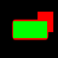
There are three issues that prevent the $F_{\beta}^{w}$ metric as defined in Section 2.2 from being directly optimized as a loss function. The first is that while the metric is differentiable almost everywhere, it is not differentiable when $y=\hat{y}$, because $\frac{d}{d\hat{y}_{i}}|\hat{y}_{i}-y_{i}|$ is undefined. In practice, we observed difficulties optimizing the error using SGD due to the constant value of the gradient for $\hat{y}\neq y$ (intuitively, because the gradient doesn’t decrease as the error decreases). We solve this by replacing the $L_{1}$ norm with $L_{2}$: $E_{i}=(\hat{y}_{i}-y_{i})^{2}$, which we find to be much easier to optimize.

The second problem is that constructing $\mathbb{A}$ (not to mention computing $E\mathbb{A}$) has $O(n^{2})$ time and space complexity. However, we can overcome this problem by leveraging convolutions. When we unpack the definition of matrix multiplication in Equation (3), we can write $E\mathbb{A}$ at pixel $i$ as:

$$\begin{split}(E\mathbb{A})_{i}&=\sum_{j}[E_{j}\mathbb{A}_{ji}]=\\ &=y_{i}\sum_{j}[y_{j}E_{j}\frac{1}{\sqrt{2\pi\sigma^{2}}}e^{\frac{-d(i,j)}{2\sigma^{2}}}]+(1-y_{i})\end{split}$$ (7)

Note that if $d(i,j)\geq 4\sigma$ then $\frac{1}{\sqrt{2\pi\sigma^{2}}}e^{\frac{-d(i,j)}{2\sigma^{2}}}\approx 0$. We then define $y_{p,q}$ and $E_{p,q}$ as the ground truth and error respectively at pixel $(p,q)$, and can approximate $(E\mathbb{A})_{i}$ as:

$$\begin{split}(E\mathbb{A})_{i}&\approx(1-y_{i})+\\ &+y_{i+(p,q)}\sum_{p,q=-4\sigma}^{4\sigma}[y\cdot E]_{i+(p,q)}\frac{1}{\sqrt{2\pi\sigma^{2}}}e^{\frac{-\sqrt{p^{2}+q^{2}}}{2\sigma^{2}}}\end{split}$$ (8)

If we let $\sigma=\frac{\theta}{4}$, we can define a $(2\theta+1)\times(2\theta+1)$ Gaussian convolutional kernel $K^{\mathbb{A}}$, yielding

$$\begin{split}E\mathbb{A}&\approx Y\odot((Y\odot E)\ast K^{\mathbb{A}})+(1-Y)\textnormal{, where}\\ K^{\mathbb{A}}_{i,j}&=\frac{1}{\sqrt{2\pi\sigma^{2}}}e^{\frac{-\sqrt{(-\theta+i)^{2}+(-\theta+j)^{2}}}{2\sigma^{2}}}\end{split}$$ (9)

Where $\odot$ is element-wise multiplication. Now we don’t need to store any entries of $\mathbb{A}$, only a$(2\theta+1)\times(2\theta+1)$ kernel and we skip most of the original summation over pixels $j$. So the time and space complexity is reduced to $O(n+\theta^{2})$. In practice, we use $\theta=9$.

The final problem is that constructing $\mathbb{B}$ has complexity $O(n^{2})$, because computing $\Delta_{i}$ requires finding the minimum $d(i,j)$ over all pixels $j$, such that $y_{j}=1$. However, if $d(i,j)\geq 25$, then $\mathbb{B}_{i}=2-e^{\alpha\cdot\Delta_{i}}\approx 2$ in Equation (4). Our intuition is that $\mathbb{B}$ is modeling the region of uncertainty about an object’s boundary, for which we believe 25 pixels to be too generous. So we redefine $\Delta_{i}$ as:

$$\Delta_{i}=\begin{cases}\infty,&\text{ if }\min_{j}d(i,j)>5\\ \min_{j}d(i,j)^{2}|y_{j}=1,&\text{ otherwise}\end{cases}$$

Squaring the distance so that the region of uncertainty is assumed to be approximately 5 pixels instead of 25. Now the time complexity is $O(n+\phi^{2})$ where $\phi=5$. We can approximate $E\odot\mathbb{B}$ using a convolution with the kernel $K^{\mathbb{B}}$, a tensor of size $\phi\times\phi\times\phi^{2}$, defined at each index (zero indexed) as:

$$K^{\mathbb{B}}_{i,j,k}=\begin{cases}(-\phi+i)^{2}+(-\phi+j)^{2},&\text{ if }k=i*(2\phi+1)+j\\ 0,&\text{otherwise}\end{cases}$$

and we can rewrite $\mathbb{B}$ as:

$$\mathbb{B}\approx Y+(1-Y)\odot e^{a\min_{k}[(Y\ast K^{\mathbb{B}})]}$$ (10)

By reformulating the local search for the true object boundary as a convolution followed by an argmin, we can leverage the efficient implmentations of these operations already available in many packages. While our current architecture does not suffer from speed or memory issues, more complicated architectures might benefit from a more optimized implementation, namely a custom ’minimization convolution’ that would not store the intermediary result of $(Y\ast K^{\mathbb{B}})$, and takes advantage of the sparsity of $K^{\mathbb{B}}$.

These changes yield a spatially informed loss function that can easily be implemented in an existing DNN framework such as Tensorflow. It fully utilizes the GPU, does not increase training wall clock time noticeably, and yields better results than more commonly used loss functions for foreground maps. Compared to an unoptimized implementation of the original formulation in python, our approximation takes two orders of magnitude less time to compute on the CPU, and three orders of magnitude less time on the GPU, to compute our loss on a 224x224 pixel image, See section 5.5.

4 Network Architecture

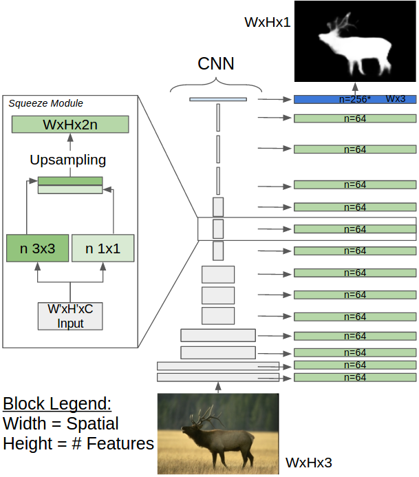
In order to produce accurate foreground maps each pixel must have a rich feature representation. To achieve this we utilize Zoomout features  [23], which have been effectively utilized in the semantic segmentation community. Zoomout features are extracted from a CNN by upsampling and downsampling the features computed by each convolutional filter to be the same spatial resolution, then concatenating the features computed at all layers of the CNN. In this way, each spatial location is richly described by both the weakly localized semantic features computed at higher layers, the strongly localized edge and color detectors computed in the first layers, and everything in between.

4.1 Squeeze Layers

Zoomout features are expressive but have a large memory footprint, limiting the spatial resolution of predictions that can be made using them. In tasks like distractor detection, where the end goal is to precisely localize distractors and remove them, a low resolution prediction leads to spatial ambiguity and lower precision. To remedy this problem we adapt the insights of [9], introducing what we call Squeeze Modules to our network. A Squeeze Module consists of $2n$ convolutional filters, $n$ of which are $1\times 1$ convolutions and $n$ of which are $3\times 3$ convolutions. Applying Squeeze Modules to each convolutional layer acts as a dimensionality reduction with learned parameters, allowing us to make predictions at essentially arbitrary resolutions by setting $n$ to be sufficiently small. In practice we produce $224\times 224$ predictions, and set $n=64$. We refer to our full architecture as a Squeezed Zoomout Network ($SZN$).

Figure 4: Architecture Diagram, note that because the blue squeeze module is applied to a fully connected layer, it uses only 1x1 convolutions.

5 Experiments

We report on experiments with three tasks where we can expect spatial sensitivity to be important for quality of the output: salient object detection, portrait segmentation, and distractor detection. See Sec. 2 for background.

5.1 Training Details

In all experiments we train our $SZN$ using a CNN (from which the squeezed zoomout features are derived) pre-trained on ImageNet. As the base CNN we use VGG-16 [28] for saliency, portraits, and distractors. We train the $SZN$ architecture using ADAM [14], and train in 3 stages. In the first stage we set the learning rate to 3e-4 for 8 epochs, In the second we set the learning rate to be 1e-4 for 4 epochs. The base CNN is kept fixed (not fine-tuned) in the first two stages. In the third stage we set the learning rate to 1e-5 for 14 epochs, fine-tuning the weights of the base CNN as well. We augment the training images by randomly permuting standard data transformations as described in [7]: image flips, random noise, changing contrast levels, and global color shifts.

5.2 Salient Object Detection

We consider four standard data sets for this task:

MSRA-B - 5000 images with pixel level annotations provided by  [12]. Widely used for salient object detection. Most images contain a single object on a high contrast background.

HKU-IS - 4447 images with pixel level annotations provided by  [17]. All images with at least one of the following attributes: multiple salient objects, salient objects touching boundary, low color contrast, complex background.

ECSSD - 1000 challenging images with pixel level annotations provided by  [32].

PASCAL-S 850 images from the PASCAL VOC 2010 segmentation challenge with pixel level annotations provided by  [18]. Following the convention of  [18] we threshold the soft labels at 0.5.

MC [33]	MDF [17]	DCL [16]	$SZN_{CE}$ (our)	$SZN_{F^{w}_{1}}$ (our)	GT	Input

Figure 5: A qualitative comparison of our method with other leading methods on object saliency. $SZN_{CE}$: our network trained with cross-entropy loss; $SZN_{F^{w}_{1}}$: our network trained with the proposed $AF^{w}_{\beta}$.

$SZN_{CE}$	$SZN_{F^{w}_{1}}$	GT	Image	$SZN_{CE}$	$SZN_{F^{w}_{1}}$	GT	Image

Figure 6: A visualization of the perceptual importance of the $F^{w}_{\beta}$ metric on object saliency. On each image, after thresholding prediction maps at 0.5, there is a less than 5% difference in the IOU score of the outputs of $SZN_{CE}$ and $SZN_{F^{w}_{1}}$, but at least a 20% percent difference in their $F^{w}_{\beta}$ score. Artifacts present in $SZN_{CE}$ outputs but alleviated in $SZN_{F^{w}_{1}}$ outputs include large interior holes, isolated blobs, and poorly defined outlines.

Evaluation Metrics

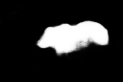
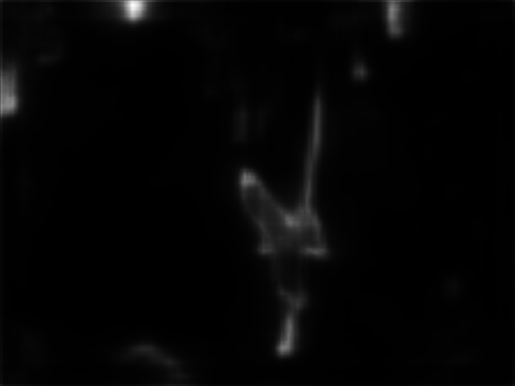
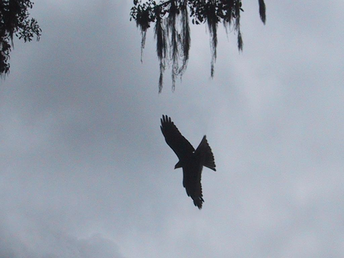
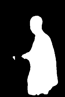
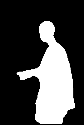
Following the convention of  [16] [17] we report the $F_{0.3}$ measure (with oracle access to the optimal threshold for the soft predictions), area under the receiver-operator characteristic curve (AUROC), and mean absolute error ($MAE=\frac{1}{W\cdot H}\sum_{i=1}^{w}\sum_{j=1}^{H}|\hat{Y}_{ij}-Y_{ij}|$). While the first two metrics evaluate whether we rank pixels correctly, MAE captures absolute classification error. We report the mean of each metrics on the test set. We also report the $F^{w}_{1}$ metric almost exactly as formulated by  [22], except that for tractibility we drop terms tied to spatially distant pixels, which are very expensive to all compute and have a negligable effect on the loss. While other measures give all errors equal weight, and a small percentage of pixels predicted differently barely affects their value, those mislabeled pixels can be perceptually vital. This is captured by the $F^{w}_{1}$ metric, we provide examples of this phenomenon in Figure  6

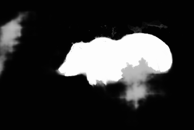
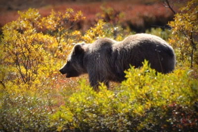
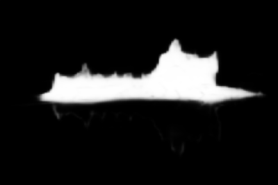
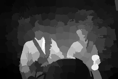
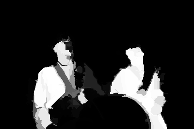
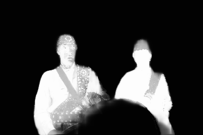
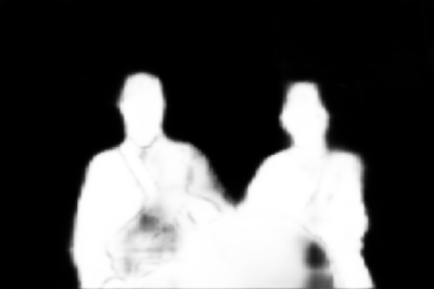
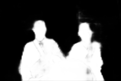
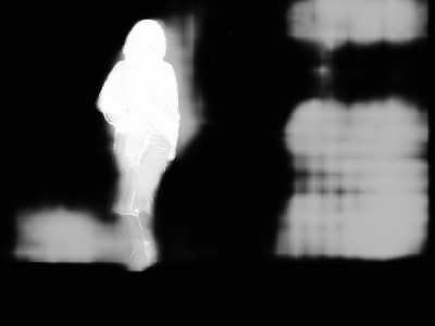
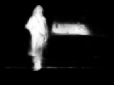
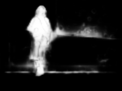
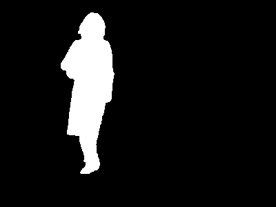
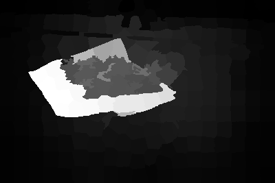
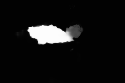
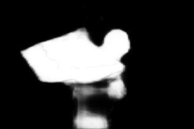
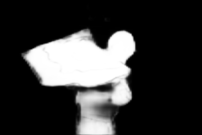
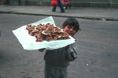
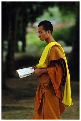
Results and Comparison Following the convention of  [16] [17] we train on 2500 images from MSRA-B, validate on 500, and test on the remaining 2000. We then use the same model trained on MSRA-B to generate predictions for all other datasets. To evaluate our proposed loss function we compare the performance of our Squeezed Zoomout Network trained with the commonly used cross-entropy loss function ($SZN_{CE}$), against the same architecture trained with the exact same training procedure, but replacing the cross entropy with our $AF^{w}_{\beta}$ loss function. The latter is our proposed method and we denote it $SZN_{F^{w}_{1}}$ from now on. We also compare both these models against other competitive techniques, MC  [33], HDHF  [17], and DCL  [16], these results are summarized in Table  1, and we provide a qualitative comparison in Figure  5 . While  [15], [31],and  [4] report competitive results on some of the same test sets, they train on 10,000 images, while we only train on 2500, making the results not directly comparable, and we omit those methods from 1.

We also use saliency to explore the effectiveness of the proposed objective function, compared to other reweighting schemes. These include: Dropping either the reweighting by the matrix $A$ or $B$, using a weighted Cross-Entropy loss, with double weight given to correctly classifying the foreground or background, and standard cross entropy, but ignoring the labels of all pixels in a 3-pixel band around the borders of the foreground. Each of these reweighting schemes reduces AUROC by close to 1%, but effect on $F^{w}_{1}$ varies. Most interesting is the large drop in performance caused by ignoring a 3-pixel border during training, which seems to indicate that these border pixels contain extremely important information for learning a higher quality model.

All inference timing results were gathered using a Titan X GPU and a 3.5GHz Intel Processor. For training MC  [33] used a Titan GPU and a 3.6GHz Intel Processor, HDHF  [17] and DCL [16] both use a Titan Black GPU and a 3.4GHz Intel Processor.

		MC	HDHF	DCL	$SZN_{CE}$	$SZN_{F^{w}_{1}}$
		[33]	[17]	[16]	ours	ours
MSRA-B	MAE	0.054	0.053	0.047	0.052	0.051
	AUC	0.975	0.982	0.983	0.987	0.988
	$F_{0.3}^{max}$	0.984	0.899	0.916	0.913	0.919
	blue!25$F^{w}_{1}$	blue!25 -	blue!25 -	blue!25 0.816	blue!25 0.829	blue!25 0.856
HKU-IS	MAE	0.102	0.066	0.049	0.057	0.057
	AUC	0.928	0.972	0.981	0.985	0.987
	$F_{0.3}^{max}$	0.798	0.878	0.904	0.891	0.904
	blue!25$F^{w}_{1}$	blue!25 -	blue!25 -	blue!25 0.768	blue!25 0.788	blue!25 0.826
ECSSD	MAE	0.100	0.098	0.075	0.069	0.073
	AUC	0.948	0.960	0.968	0.981	0.980
	$F_{0.3}^{max}$	0.837	0.856	0.924	0.905	0.908
	blue!25$F^{w}_{1}$	blue!25 -	blue!25 -	blue!25 0.767	blue!25 0.796	blue!25 0.827
PASCAL-S	MAE	0.145	0.142	0.108	0.106	0.109
	AUC	0.907	0.922	0.924	0.954	0.954
	$F_{0.3}^{max}$	0.740	0.781	0.822	0.833	0.839
	blue!25$F^{w}_{1}$	blue!25 -	blue!25 -	blue!25 0.670	blue!25 0.657	blue!25 0.680
Train Speed		19H	12H	15H	4 H
Test Speed		1.1s	2.5s	0.88s	0.094s

Table 1: Quantitative comparisons between our approach and other leading methods. MAE and - lower is better; AUC, $F_{0.3}^{max}$, and $F^{w}_{1}$ - higher is better. Italics indicate a projected training speedup of 1.67 if run on our hardware

	MTurk	Dist9
[8]	0.81	0.67
Ours	0.84	0.87
Human	0.89	-

Table 2: Comparison with Fried et al. [8] on distractor detection.

Figure 7: Distractor detection results across different categories in Dist9 dataset

	MIoU	$F^{w}_{1}$	Test Speed
$PFCN$ [26]	94.20	0.965	0.114s
$PFCN+$ [26]	95.91	0.972	1.125s
$SZN_{CE}$	96.53	0.965	0.036s
$SZN_{F^{w}_{1}}$	97.13	0.973	0.036s

Table 3: Portrait segmentation results. $PortraitFCN+$  [26] augments images with 3 extra channels, See text for details.

	AUROC	$F^{w}_{1}$
Proposed	0.988	0.856
Proposed, no A	0.976	0.836
Proposed, no B	0.975	0.835
Cross-Entropy, 2x foreground weight	0.976	0.834
Cross-Entropy, 2x background weight	0.974	0.797
Cross-Entropy, 3pix ’DNC’ band	0.973	0.807

Table 4: Objective function comparison, see text for details

5.3 Portrait Segmentation

Dataset We use the dataset from [26], consisting of 1800 human portrait images gathered from Flickr. A face detector is run on each image, producing a centered crop scaled to be an 800x600. The crop is manually segmented using Photoshop’s “quick select”. This dataset focuses on portraits captured using a front-facing mobile camera (through the choice of Flickr queries), but includes other portrait types as well. The dataset is split into 1500 training images and 300 test images. There is a wide variety in the subjects’ age, clothing, accessories, hair-style, and background.

Results Table 3 shows that by MIoU both our models significantly outperform $PFCN$ (PortraitFCN), which uses only RGB input; and $PFCN+$, which requires substantial preprocessing (fiducial point detection, computing an average segmentation mask and aligning it to the input face location) and additional input channels. While our $SZN_{F^{w}_{1}}$ model achieves significantly higher $F^{w}_{1}$ scores than $PFCN$ and $SZN_{CE}$, they are only slightly better than $PFCN+$. We believe this is due to the spatial guidance used by $PFCN+$.

5.4 Distractor Detection

Datasets

MTurk - A dataset of 403 images, with accurate, pixel level annotations averaged over many (on average 27.8  [8]) humans through Mechanical Turk.

Dist9 - A dataset of 4019 images, gathered via a free app which removed regions highlighted by users. Because the ground truth was gathered based on thumb swipes it is often inexact, and has only weak correspondence with object boundaries. To rectify this we used ground truth with scores averaged over super pixels generated with MCG  [3], where the boundary threshold is set to be 0.1. In this dataset each pixel is labeled with either one of 9 foreground classes corresponding to different types of distractors (light, object, person, clutter, pole, trash, sign, shadow, and reflection) or background.

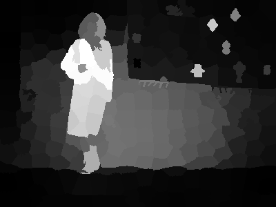
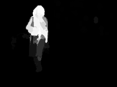
Evaluation We evaluate our performance on the MTurk dataset through 10 fold cross validation, and compare against the performance of [8] using leave-one-out cross validation. Note that this disadvantages our method, because while each model they use for validation is trained on 402 images, each model we use is trained on 362 or 363 images. We also compare against [8] on the Dist9 dataset, training 10 separate models, one on the entire dataset, and one each of the 9 small datasets corresponding to one of the foreground classes. We split the dataset randomly, using 90% to train and 10% to test. Following the convention of  [8], we measure AUROC on all datasets. The results are summarized in Table  2, and Figure  7. Note the final column in Figure  7 averages across categories, while Table  2 averages over the entire dataset.

5.5 Approximation speed

To evaluate the relative speed of our approximation we compute wall clock time of computing the $F^{w}_{\beta}$, and $AF^{w}_{\beta}$ scores, averaged on fifteen random images from ECSSD. While the original $F^{w}_{\beta}$ takes 37 minutes, our approximation takes 8.7 seconds on a cpu, and 0.33 seconds on a GPU.

6 Discussion and Future Work

We propose a differentiable and efficient objective function which directly encoding multiple widely desirable spatial properties of a foreground mask. We use this objective to learn the parameters of a novel “squeezed zoomout” architecture. resulting in high fidelity foreground maps, which match or surpass state of the art results for a range of binary segmentation tasks. Notably, we achieve these results without relying on any pre-processing (e.g., super-pixel segmentation) or post-processing (e.g., CRF). An interesting direction for fugure work is to generalize our loss function to a multi-class setting, for instance semantic segmentation.

References

- [1] R. Achanta, S. Hemami, F. Estrada, and S. Susstrunk. Frequency-tuned salient region detection. In Computer vision and pattern recognition, 2009. cvpr 2009. ieee conference on, pages 1597–1604. IEEE, 2009.
- [2] F. Ahmed, D. Tarlow, and D. Batra. Optimizing expected intersection-over-union with candidate-constrained crfs. In Proceedings of the IEEE International Conference on Computer Vision, 2015.
- [3] P. Arbeláez, J. Pont-Tuset, J. T. Barron, F. Marques, and J. Malik. Multiscale combinatorial grouping. In Proceedings of the IEEE Conference on Computer Vision and Pattern Recognition, pages 328–335, 2014.
- [4] S. Chandra and I. Kokkinos. Deep, dense, and low-rank gaussian conditional random fields. arXiv preprint arXiv:1611.09051, 2016.
- [5] K.-Y. Chang, T.-L. Liu, H.-T. Chen, and S.-H. Lai. Fusing generic objectness and visual saliency for salient object detection. In 2011 International Conference on Computer Vision, pages 914–921. IEEE, 2011.
- [6] M.-M. Cheng, N. J. Mitra, X. Huang, P. H. Torr, and S.-M. Hu. Global contrast based salient region detection. IEEE Transactions on Pattern Analysis and Machine Intelligence, 37(3):569–582, 2015.
- [7] A. Dosovitskiy, P. Fischer, E. Ilg, P. Häusser, C. Hazirbas, V. Golkov, P. van der Smagt, D. Cremers, and T. Brox. Flownet: Learning optical flow with convolutional networks. In 2015 IEEE International Conference on Computer Vision, ICCV 2015, Santiago, Chile, December 7-13, 2015, pages 2758–2766, 2015.
- [8] O. Fried, E. Shechtman, D. B. Goldman, and A. Finkelstein. Finding distractors in images. In Proceedings of the IEEE Conference on Computer Vision and Pattern Recognition, pages 1703–1712, 2015.
- [9] F. N. Iandola, M. W. Moskewicz, K. Ashraf, S. Han, W. J. Dally, and K. Keutzer. Squeezenet: Alexnet-level accuracy with 50x fewer parameters and¡ 1mb model size. arXiv preprint arXiv:1602.07360, 2016.
- [10] M. Jansche. Maximum expected f-measure training of logistic regression models. In Proceedings of the conference on Human Language Technology and Empirical Methods in Natural Language Processing, pages 692–699. Association for Computational Linguistics, 2005.
- [11] Y. Jia and M. Han. Category-independent object-level saliency detection. In Proceedings of the IEEE international conference on computer vision, pages 1761–1768, 2013.
- [12] H. Jiang, J. Wang, Z. Yuan, Y. Wu, N. Zheng, and S. Li. Salient object detection: A discriminative regional feature integration approach. In Proc. IEEE Conference on Computer Vision and Pattern Recognition, 2013.
- [13] T. Judd, K. Ehinger, F. Durand, and A. Torralba. Learning to predict where humans look. In 2009 IEEE 12th International Conference on Computer Vision, pages 2106–2113. IEEE, 2009.
- [14] D. P. Kingma and J. Ba. Adam: A method for stochastic optimization. CoRR, abs/1412.6980, 2014.
- [15] I. Kokkinos. Ubernet: Training auniversal’convolutional neural network for low-, mid-, and high-level vision using diverse datasets and limited memory. arXiv preprint arXiv:1609.02132, 2016.
- [16] G. Li and Y. Yu. Deep contrast learning for salient object detection. arXiv preprint arXiv:1603.01976, 2016.
- [17] G. Li and Y. Yu. Visual saliency detection based on multiscale deep cnn features. IEEE Transactions on Image Processing, 25(11):5012–5024, 2016.
- [18] Y. Li, X. Hou, C. Koch, J. M. Rehg, and A. L. Yuille. The secrets of salient object segmentation. In Proceedings of the IEEE Conference on Computer Vision and Pattern Recognition, pages 280–287, 2014.
- [19] T. Liu, Z. Yuan, J. Sun, J. Wang, N. Zheng, X. Tang, and H.-Y. Shum. Learning to detect a salient object. IEEE Transactions on Pattern analysis and machine intelligence, 33(2):353–367, 2011.
- [20] J. Long, E. Shelhamer, and T. Darrell. Fully convolutional networks for semantic segmentation. CoRR, abs/1411.4038, 2014.
- [21] Y.-F. Ma and H.-J. Zhang. Contrast-based image attention analysis by using fuzzy growing. In Proceedings of the eleventh ACM international conference on Multimedia, pages 374–381. ACM, 2003.
- [22] R. Margolin, L. Zelnik-Manor, and A. Tal. How to evaluate foreground maps? In CVPR, 2014.
- [23] M. Mostajabi, P. Yadollahpour, and G. Shakhnarovich. Feedforward semantic segmentation with zoom-out features. In Proceedings of the IEEE Conference on Computer Vision and Pattern Recognition, pages 3376–3385, 2015.
- [24] S. Nowozin. Optimal decisions from probabilistic models: the intersection-over-union case. In Proceedings of the IEEE Conference on Computer Vision and Pattern Recognition, 2014.
- [25] N. Rosenfeld, O. Meshi, D. Tarlow, and A. Globerson. Learning structured models with the auc loss and its generalizations. In AISTATS, 2014.
- [26] X. Shen, A. Hertzmann, J. Jia, S. Paris, B. Price, E. Shechtman, and I. Sachs. Automatic Portrait Segmentation for Image Stylization. Computer Graphics Forum, 2016.
- [27] X. Shen and Y. Wu. A unified approach to salient object detection via low rank matrix recovery. In IEEE Conference on Computer Vision and Pattern Recognition (CVPR’12), 2012.
- [28] K. Simonyan and A. Zisserman. Very deep convolutional networks for large-scale image recognition. arXiv preprint arXiv:1409.1556, 2014.
- [29] P. Viola and M. Jones. Rapid object detection using a boosted cascade of simple features. In Proc. of of the IEEE Conference Computer Vision and Pattern Recognition, volume 1, 2001.
- [30] L. Wang, H. Lu, X. Ruan, and M.-H. Yang. Deep networks for saliency detection via local estimation and global search. In Proceedings of the IEEE Conference on Computer Vision and Pattern Recognition, pages 3183–3192, 2015.
- [31] X. Xi, Y. Luo, F. Li, P. Wang, and H. Qiao. A fast and compact salient score regression network based on fully convolutional network. arXiv preprint arXiv:1702.00615, 2017.
- [32] Q. Yan, L. Xu, J. Shi, and J. Jia. Hierarchical saliency detection. In Proc. of the IEEE Conference on Computer Vision and Pattern Recognition, 2013.
- [33] R. Zhao, W. Ouyang, H. Li, and X. Wang. Saliency detection by multi-context deep learning. In Proceedings of the IEEE Conference on Computer Vision and Pattern Recognition, pages 1265–1274, 2015.
- [34] W. Zhu, S. Liang, Y. Wei, and J. Sun. Saliency optimization from robust background detection. In Proceedings of the IEEE conference on computer vision and pattern recognition, pages 2814–2821, 2014.