Möbius Moduli for Fingerprint Orientation Fields

Abstract

We propose a novel fingerprint descriptor, namely Möbius moduli, measuring local deviation of orientation fields (OF) of fingerprints from conformal fields, and we propose a method to robustly measure them, based on tetraquadrilaterals to approximate a conformal modulus locally with one due to a Möbius transformation. Conformal fields arise by the approximation of fingerprint OFs given by zero pole models, which are determined by the singular points and a rotation. This approximation is very coarse, e.g. for fingerprints with no singular points (arch type), the zero-pole model’s OF has parallel lines. Quadratic differential (QD) models, which are obtained from zero-pole models by adding suitable singularities outside the observation window, approximate real fingerprints much better. For example, for arch type fingerprints, parallel lines along the distal joint change slowly into circular lines around the nail furrow. Still, QD models are not fully realistic because, for example along the central axis of arch type fingerprints, ridge line curvatures usually first increase and then decrease again. It is impossible to model this with QDs, which, due to complex analyticity, also produce conformal fields only. In fact, as one of many applications of the new descriptor, we show, using histograms of curvature and conformality index (log of the absolute value of the Möbius modulus), that local deviation from conformality in fingerprints occurs systematically at high curvature which is not reflected by state of the art fingerprint models as are used, for instance, in the well known synthetic fingerprint generation tool SFinGe and these differences robustely discriminate real prints from SFinGe’s synthetic prints.

Keywords

Fingerprint recognition, orientation field modeling, Möbius transformation, conformal modulus, quadratic differentials, zero-pole model, Riemann mapping theorem

MSC Class

Primary: 62P10
Secondary: 30C62

1 Introduction

Fingerprints are usually described by features at several levels. At the first level there is the orientation field, at the second there are minutiae and ridge frequencies and at the third there are pores etc., for an overview see for instance Maltoni et al. (2009). In this paper we introduce a new feature at the second level which has previously not been studied. It is a local feature of the orientation field and we call it the Möbius modulus. The log of its absolute value is the conformality index. These terms are motivated from the theory of complex functions and in particular from the Riemann mapping theorem.

Informally, our new feature can be understood as follows. Fix two points $p_{1}$ and $p_{2}$ on a common fingerprint ridge, uniformly heat up this ridge segment and follow the diffusion of heat orthogonal to the orientation field. If heat level curves agree with neighboring ridge lines (as in Figure 1), we say that the field is locally conformal, and indeed, it turns out that fingerprints are locally conformal to large extent. If the ridge lines no longer agree with heat level curves (as in Figure 2), we say that the field is locally non-conformal. In this paper we make these concepts precise and propose a method to locally measure the degree of conformality of fingerprint orientation fields outside neighborhoods of the singular points. At this point we note that in view of application and audience, we resort to the lean notion of conformal and non-conformal fields, where in the language of Riemann surfaces (e.g. Strebel (1984)) we refer to a conformal structure equivalent or not equivalent to that induced by the conformal structure of the Riemann sphere.

This new feature, the conformality index, has several applications. In this paper we show that curvature combined with this new feature is highly discriminatory for distinguishing real fingerprints from fingerprints synthetically generated by SFinGe.

There are other applications of Möbius moduli and the conformality index of which we mention the following. In Huckemann et al. (2008) we have introduced quadratic differentials as global models for orientation fields of fingerprints. They are generalizations of zero pole models from Sherlock and Monro (1993), and such models yield conformal fields, by their very definition via meromorphic functions. Since orientation fields of real fingerprints also feature non-conformality, in order to obtain an asymptotically perfectly fitting orientation field, in the low parameter representation of Gottschlich et al. (2017), one may precisely feed in the loci of highest deviation from conformality. This gives a natural low dimensional feature vector, which can be used for fast indexing. As another application, e.g. to latent fingerprint matching, knowledge about the joint curvature and conformality index distribution may be used to enhance the orientation field of bad quality latents and infer on the orientation field at bad quality or unobserved locations, e.g Huckemann et al. (2008); Bartůněk et al. (2013). Further potential applications lie in aiding matching and alignment of fingerprints. In conclusion we remark that correlation between curvature and non-conformality may add essential understanding to embryonic growth models, e.g. Kücken and Champod (2013), which are to date not fully satisfactory.

2 Conformal Maps and Quadratic Differentials

The following can be found in any standard textbook on complex analysis, e.g. Ahlfors (1966), and on quadratic differentials, e.g. Strebel (1984). A complex mapping $x+iy=z\mapsto f(z)$ is conformal if it is partially differentiable with

$$f^{\prime}(z)=\frac{\partial f}{\partial z}=\frac{1}{2}\left(\frac{\partial f(x+iy)}{\partial x}-i\frac{\partial f(x+iy)}{\partial y}\right)\neq 0$$

and if it satisfies the Cauchy-Riemann differential equations

$$\frac{\partial f}{\partial\bar{z}}=\frac{1}{2}\left(\frac{\partial f(x+iy)}{\partial x}+i\frac{\partial f(x+iy)}{\partial y}\right)=0\,.$$

The Riemann Mapping Theorem

asserts that every simply connected open set $G$ that is a proper subset of the complex plane $\mathbb{C}$ can be mapped conformally onto any open rectangle $R_{\tau}=\{w\in\mathbb{C}:0<\,{\rm Re}(w)<1,~{}0<\,{\rm Im}(w)<\tau\}$. More precisely, for every selection of four distinct points $p_{1},\ldots,p_{4}\in\partial G$ on the boundary of $G$ in positive cyclic positive order, there is a unique $\tau>0$ and a unique conformal map $f:G\to R_{\tau}$ such that

$$p_{1}\mapsto 0,p_{2}\mapsto 1,p_{3}\mapsto 1+i\tau\mbox{ and }p_{4}\mapsto i\tau\,.$$ (1)

The simply connected open set $G$ with these four points is a quadrilateral and $\tau=\tau(G)$ is its modulus, cf. Figures 1 and 2. In order to obtain the conformal mapping $f$ we introduce quadratic differentials.

A quadratic differential

(QD) $\sigma$ on a subset $D$ of the Riemann sphere $\hat{\mathbb{C}}=\mathbb{C}\cup\{\infty\}$ is a mapping from the tangent bundle $TD$ into $\hat{\mathbb{C}}$ such that

$$\sigma(z,dz)=Q(z)\,dz^{2}$$

with a function $Q$ meromorphic in $D$, i.e. complex analytic except for possible isolated poles. A trajectory of $\sigma$ is a curve $t\mapsto\gamma(t)$ on which $\sigma\big{(}\gamma(t),\dot{\gamma}(t)\big{)}>0$, on an orthogonal trajectory, $\sigma<0$.

If $G$ is a quadrilateral defined by four boundary points $p_{1},\ldots,p_{4}$ with modulus $\tau$, and if $\sigma(z,dz)=Q(z)\,dz^{2}$ is a quadratic differential, with $Q$ holomorphic in $G$, and trajectories on the boundary of $G$ between $p_{1}$ and $p_{2}$ as well as between $p_{3}$ and $p_{4}$, and with orthogonal trajectories on the boundary of $G$ between $p_{2}$ and $p_{3}$ as well as between $p_{4}$ and $p_{0}$, then the above conformal map $f:G\to R_{\tau}$ with boundary correspondence (1) is given by

$$f(z) = \int_{p_{1}}^{z}\sqrt{Q(\zeta)}\,d\zeta\,,$$ (2)

with a suitable branch of the root, cf. Figure 1. This results from the differential equation

$$dw^{2}=\big{(}df(z)\big{)}^{2}=Q(z)\,dz^{2}$$

and the fact that all vertical lines are trajectories of $dw^{2}$, and that horizontal lines are orthogonal trajectories, cf. Figure 1.

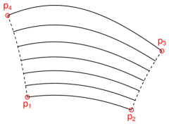
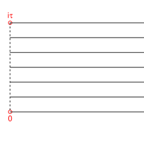
$z$                      $\longrightarrow$                      $w$

Figure 1: Conformally mapping a quadrilateral with conformal OF from the $z$ plane (left) onto a rectangle in the $w$ plane (right). Trajectories of $dw^{2}>0$ and their pre-images are depicted by solid lines, orthogonal trajectories by dashed lines.

Circles and Möbius transformations.

A specific class of conformal mappings is given by Möbius transformation which have the form

$$z\mapsto f(z) = \frac{az+b}{cz+d}\,,$$ (3)

with suitable parameters $a,b,c,d\in\mathbb{C}$ satisfying $ad-bc\neq 0$. These map $\hat{\mathbb{C}}$ conformally onto itself so that in particular, circles are mapped to circles. Here, a circle in $\hat{\mathbb{C}}$ is either a proper circle in $\mathbb{C}$ or a straight line which is then viewed as a circle through $z=\infty$.

In this terminology, the trajectories of $dw^{2}$ are then circles passing parallel through $\infty$. Also the orthogonal trajectories of $dw^{2}$ are circles passing parallel through $\infty$ but orthogonal to the trajectories.

3 Deviation from Conformality

Definition.

Suppose that we are given an orientation field (OF), arising from a fingerprint, say, in a simply connected domain $G$. This means that its singular points are isolated in $G$ and every non-singular point $z\in G$ carries a unique orientation $dz^{2}\in\mathbb{C}\setminus\{0\}$. A trajectory of the OF is a maximal, differentiable curve $t\mapsto\gamma(t)=z$ through non-singular points such that $(\dot{\gamma}(t)/dz)^{2}>0$. Similarly, for an orthogonal trajectory we have $(\dot{\gamma}(t)/dz)^{2}<0$.

For such OFs in $G$ we say that a quadrilateral $G_{p_{1},p_{2},p_{3},p_{4}}\subset G$ is a subquadrilateral if

• its closure comprises non-singular points only,

• its boundary comprises arcs of trajectories between $p_{1},p_{2}$ as well as between $p_{3},p_{4}$ and arcs on orthogonal trajectories between $p_{2},p_{3}$ as well as between $p_{4},p_{1}$,

• $p_{1},p_{2},p_{3},p_{4}$ are in cyclic positive order w.r.t. $G_{p_{1},p_{2},p_{3},p_{4}}$.

Under the mapping $f$ from (2) this subquadrilateral is mapped onto a rectangle with suitable modulus $\tau$. As elaborated in the preceding section, if the OF stems from a QD, under $f$ all trajectories of the OF are mapped to horizontal lines. If this is not the case, we say that the OF deviates from conformality, cf. Figure 2.

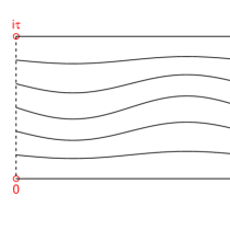
$z$                      $\longrightarrow$                      $w$

Figure 2: Mapping a quadrilateral with a non-conformal OF conformally onto a rectangle.

Measuring.

In order to measure deviation from conformality several methods come to mind. One could measure, say, in the $w$-plane,

• maximal vertical aberration of trajectory images from horizontal lines,

• or maximal curvature of trajectory images.

These and similar method require in particular the numerical computation of the integral in (2), a numerically highly challenging problem.

In a first approximation, one might replace the trajectory arcs of the OF with circular arc segments giving a circular arc rectangle. Then the integral in (2) could be analytically solved by taking recourse to the circular version of the Schwarz-Christoffel Formula. This formula, however, as is well known, is numerically highly unstable, cf. Trefethen (2002).

The Möbius approximation.

In a second approximation we replace the trajectory and orthogonal trajectory arcs on the boundary of $G_{p_{1},p_{2},p_{3},p_{4}}$ with specific circular arc segments, mimicking the trajectory and orthogonal trajectory structure of $dw^{2}$ as discussed above, such that the corresponding circles intersect at a common point in $\hat{\mathbb{C}}$ where the circles determined by $p_{1},p_{2}$ and $p_{3},p_{4}$ are parallel and orthogonal to the circles determined by $p_{2},p_{3}$ and $p_{4},p_{1}$, which are also parallel there. Then the conformal mapping $f$ from (2) is simply a Möbius transformation given by (3). In this case the modulus of $G_{p_{1},p_{2},p_{3},p_{4}}$ is given by the double cross-ratio

$$\tau(G_{p_{1},p_{2},p_{3},p_{4}}) = \frac{p_{1}-p_{2}}{p_{1}-p_{4}}~{}\frac{p_{3}-p_{4}}{p_{3}-p_{2}}\,.$$ (4)

For general subquadrilaterals $G_{p_{1},p_{2},p_{3},p_{4}}$ denote the right hand side of (4) by

$$M(G_{p_{1},p_{2},p_{3},p_{4}}) := \frac{p_{1}-p_{2}}{p_{1}-p_{4}}~{}\frac{p_{3}-p_{4}}{p_{3}-p_{2}}\,.$$ (5)

Figure 3 shows the general case of a circular arc rectangle and its Möbius approximation.

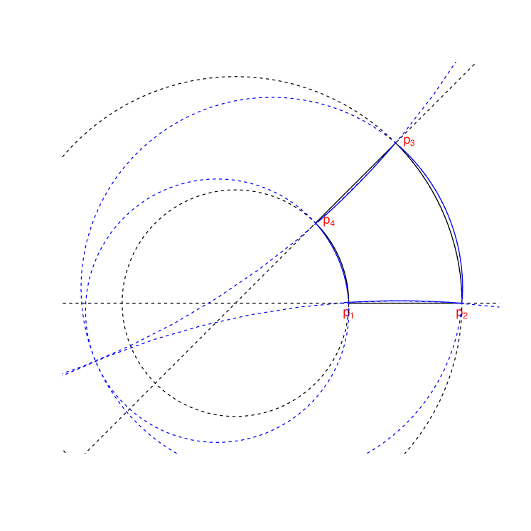
Figure 3: A circular arc rectangle (black) formed by two intersecting lines and two concentric circles and its Möbius approximation (blue) formed by two pairs of circles, each pair is tangential at a common point and intersecting the other pair orthogonally there. Both circular arc rectangles have the same vertex points $p_{1},p_{2},p_{3},p_{4}$ where the corresponding circles intersect orthogonally.

Tetraquadrilaterals and Möbius moduli.

In order to propose a simple measure for the degree of conformality, we subdivide a given subquadrilateral $G_{p_{1},p_{2},p_{3},p_{4}}$ of an OF into four smaller subquadrilaterals, determined by picking an arbitrary but fixed point $q_{0}\in G_{p_{1},p_{2},p_{3},p_{4}}$. Then the OF’s trajectory through $q_{0}$ intersects the orthogonal trajectories between $p_{1},p_{4}$ in a point $q_{1}$ and between $p_{2},p_{3}$ in a point $q_{3}$, respectively and the OF’s orthogonal trajectory through $q_{0}$ intersects the trajectories between $p_{1},p_{2}$ in a point $q_{2}$ and between $p_{3},p_{4}$ in a point $q_{4}$, respectively, cf. Figure 4. We call this subdivision into four subquadrilaterals a tetraquadrilateral (TQL) centered at $q_{0}$. We apply the Möbius approximation jointly to each of the four subquadrilaterals, i.e. we assume that all trajectories are on circles that touch at a common point in $\hat{\mathbb{C}}$ with tangent orthogonal to the tangent of the circles on which the orthogonal trajectories lie, that touch at the same point. Then the cross-ratio of moduli – we take the approximation $M$ given by (5) – gives rise to the Möbius modulus

$$M(G_{p_{1},p_{2},p_{3},p_{4}},q_{0}) = \frac{M(G_{p_{1},q_{2},q_{0},q_{1}})}{M(G_{q_{2},p_{2},q_{3},q_{0}})}~{}\frac{M(G_{q_{0},q_{3},p_{3},q_{4}})}{M(G_{q_{1},q_{0},q_{4},p_{4}})}$$ (6)

$$= \frac{p_{1}-q_{2}}{q_{2}-p_{2}}~{}\frac{p_{2}-q_{3}}{q_{3}-p_{3}}~{}\frac{p_{3}-q_{4}}{q_{4}-p_{4}}~{}\frac{p_{4}-q_{1}}{q_{1}-p_{1}}\,.$$

This is a complex number that only vanishes in degenerate scenarios which we have excluded by definition. If the Möbius approximation holds true and if the OF is conformal, then $M(G_{p_{1},p_{2},p_{3},p_{4}},q_{0})=1$. Otherwise, $\log M$ gives in approximation the deviation from conformality.

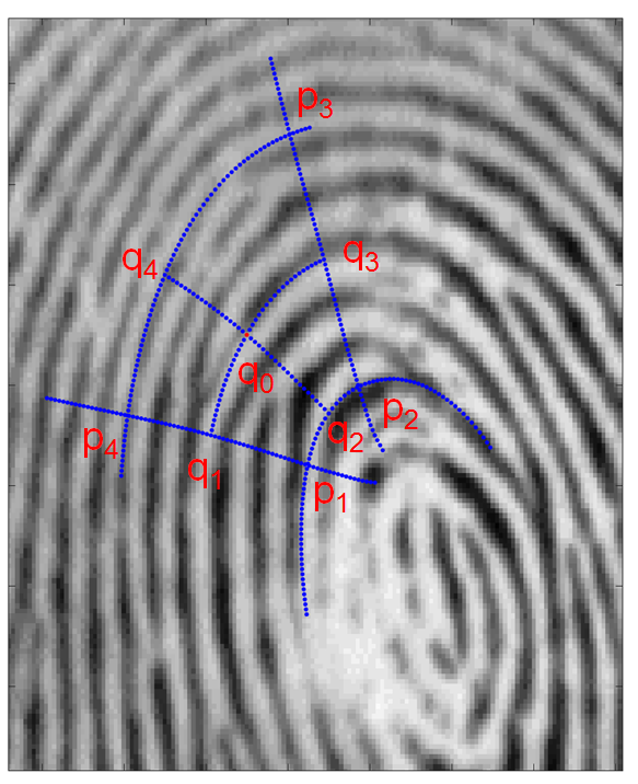
Figure 4: A tetraquadrilateral obtained from choosing the point $q_{0}$ within a subquadrilateral.

Simulations with OFs stemming from QDs show that the Möbius approximation is quite good. In fact, below it serves surprisingly well to identify areas of deviation from conformality of real and synthetic fingerprints.

Visualizing Möbius moduli of tetraquadrilaterals.

From equation (6) we see that the Möbius modulus $M=me^{i\phi}$ of a TQL is determined by the ratios of subsequent boundary segments. The logarithm of its absolute value, $\log m$, called the conformality index, reflects the ratio of the lengths and its argument $\phi$ reflects the sum and differences of the angles, cf. Figure 5. In the application of this contribution we only consider the conformality index.

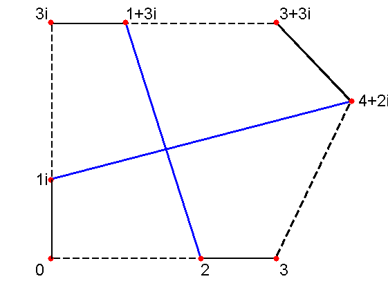
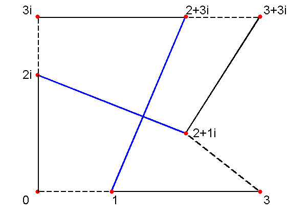
Figure 5: Visualizing the Moebius modulus $M=me^{i\phi}$ of a TQL. Under conformality $M=1$, if the Möbius approximation is exact. Left: Positive $\log m$ and $\phi\in(-\pi,0)$. Right: Negative $\log m$ and $\phi\in(0,\pi)$.

4 Estimating Möbius Moduli in Fingerprints

Fingerprint segmentation Thai et al. (2016); Thai and Gottschlich (2016) into foreground, the region of interest (ROI), and background, as well as orientation field estimation by a combination of the line sensor Gottschlich et al. (2009) and gradient based method as described in Gottschlich and Schönlieb (2012), say, are the first two typical processing steps in fingerprint algorithms. For a given fingerprint image with estimated ROI and orientation field, in order to define TQLs, we use the curved regions of Gottschlich (2012): A TQL centered at $q_{0}$ in the ROI can be obtained as follows. From $q_{0}$ traverse the OF in either direction with a fixed length $c=40$ pixels (approximately 3 ridge distances) and the orthogonal OF also in either direction with same lengths $c$. This gives the black cross in Figure 6. From the endpoints of that cross, traverse the OF in either direction (red in Figure 6), or the orthogonal OF in either direction (light blue in Figure 6), respectively, until the corresponding curves meet. The four intersection points together with the four crosses’ endpoints and $q_{0}$ form the TQL. We compute TQLs centered at every pixel locus $q_{0}$ over the entire ROI.

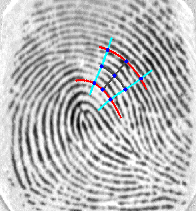
Figure 6: Stepwise building a TQL: First an equal sided cross aligned with the OF about the central point (grey), then traversing along trajectories (red) and orthogonal trajectories (light blue), respectively, from the endpoints, until intersection points are reached. These intersection points, with the crosses endpoints and the central point give the TQL (dark blue).

If in the process of the above routine, trajectories or orthogonal trajectories leave the ROI, no TQL is computed. Moreover, two problems can occur, when attempting to determine TQLs close to singular points, and also in these cases, no TQLs are computed. First, it may happen that orthogonal and non-orthogonal trajectories turn away from one another, and hence, have no intersection points, as depicted in Figure 7 (left panel). Secondly, high curvature can lead to self intersecting lines, say, of the central cross in Figure 7 (right panel), so that no meaningful TQL can be defined.

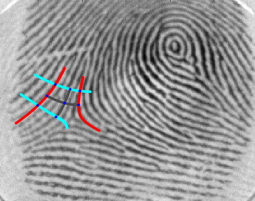
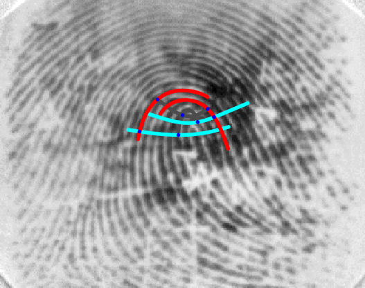
Figure 7: Building a TQL close to a singular point may fail if trajectories turn away from one another, near a delta (left), or self intersect, near a core (right).

5 Synthetic Fingerprint Generation

The generation of synthetic fingerprints is of great interest to the biometric and forensic community. Fingerprint databases are required for evaluating and comparing the performance of algorithms for minutiae extraction, fingerprint verification, fingerprint indexing and identification. In the following, we focus on artificially generated fingerprint images. A very related but different topic is fingerprint liveness detection, the discrimination between images of real, alive fingers and images of spoof fingers made from material like gelatin, wood glue or silicone (see Gottschlich (2016) for a recent survey on fingerprint liveness detection).

Major advantages of synthetic fingerprints are given by the fact that millions of prints can be created at virtually no cost and their generation is not hindered by national laws and legal constraints concerning data protection and privacy. However, artificial fingerprints have to be ’realistic’, or otherwise the validity of results obtained on databases of synthetic prints can be called into question. In 2014, a study showed that the methods for fingerprint generation at that time produced prints with an unrealistic minutiae distributions Gottschlich and Huckemann (2014): Distances between minutiae locations and angles between minutiae directions, summarized in minutiae histograms (MHs) Gottschlich and Huckemann (2014) for minutiae pairs had been compared by the earth movers’ distance (EMD) Gottschlich and Schuhmacher (2014).

Methods for creating artificial fingerprint include SFinGe by Cappelli et al. Cappelli et al. (2000) and Araque et al. Araque et al. (2002). Both algorithms utilize a global orientation field model by Vizcaya and Gerhardt Vizcaya and Gerhardt (1996). Images created by SFinGe are part of the widely used FVC databases.

While previously minutiae have been used to separate real from synthetic fingerprints Gottschlich and Huckemann (2014), the experiments and results described in the next section are based on the orientation field only.

SFinGe has also been used in comparison of fingerprint classification methods by Galar et al. Galar et al. (2015a, b). Most classification methods utilize the orientation field, and hence, these results are based on unrealistic OFs as will be shown in the next section.

Recently, a novel method for fingerprint generation has been proposed Imdahl et al. (2015) which overcomes the aforementioned problems. The realistic fingerprint creator (RFC) Imdahl et al. (2015) utilizes orientation fields from real fingerprints and templates are checked whether they pass the ’test of realness’ Gottschlich and Huckemann (2014) for minutiae distribution.

6 Discriminating Real from Synthetic Prints by Histograms of Möbius Moduli and Curvatures

Möbius moduli and curvature Gottschlich (2012) are computed as described in Section 4. Then a 2D histogram summarizes the joint distribution of curvature and conformality indices (logs of absolute values of Möbius moduli) for every foreground pixel for which a TQL was computed.

These 2D histograms with 10 bins, and with 20 bins, for each dimension, are considered as feature vectors with 100 and 400 entries, respectively, and these feature vectors are used for training by a support vector machine with a linear kernel ($C=1.0$). Experimental results listed in Table 1 have been obtained using the software package LIBSVM Chang and Lin (2011).

Each FVC database contains images from 110 fingers with 8 impressions per finger. Each competition in 2000, 2002 and 2004 contains one synthetic database (DB 4) which we have paired with one real database (DB 1) from the same year. From 110 available fingers, 60 real and 60 synthetic are assigned into the training set and the remaining 50 real and 50 synthetic into the test set.

	10 bins, one impression			20 bins, one impression
FVC	2000	2002	2004	2000	2002	2004
Training set	96.7%	98.3%	97.5%	100%	100%	100%
Test set	76%	73%	70%	74%	80%	75%
	10 bins, eight impressions			20 bins, eight impressions
FVC	2000	2002	2004	2000	2002	2004
Training	100%	100%	100%	100%	100%	100%
Test set	100%	100%	100%	100%	100%	100%

Table 1: SVM classification accuracy of 2D histograms using 10 (left) and 20 bins (right) for each of the two dimensions, Möbius moduli and curvature. The results in the upper half summarize histograms per one impression, in the lower half, histograms per eight impressions.

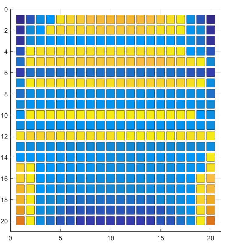
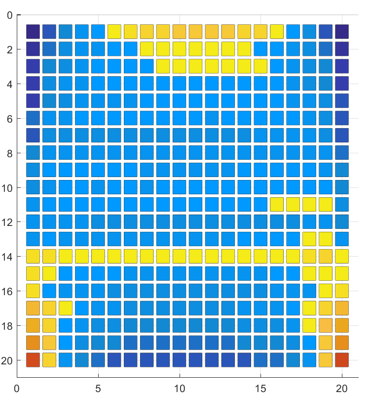
Figure 8: Averaged histograms of conformality indices (horizontal, zero in the middle and $\pm 0.33$, and beyond, at the ends) vs. curvature (vertical, zero on top, $2.6$, and beyond, at the bottom) for FVC 2000 (left column), FVC 2002 (middle column) and FVC 2004 (right column). Top row: Real fingerprints. Bottom row: Synthetic fingerprints.

7 Discussion

In Figure 8 we see that for real fingerprints (top row), extremal conformality indices (first and last histogram columns) strongly peak at high curvature (bottom histogram rows), whereas for synthetic prints, these peaks are far less pronounced. These systematic differences are also visible in Figure 9. Upon closer inspection note that high curvature regions form similar clusters for both types of prints, these clusters, however, split into two extremal non-conformality clusters, only for real prints, like rabbit ears. These rabbit ears indicate that above cores and above and below whorls, real fingerprints are locally more bent or distorted than as predicted by the corresponding zero-pole model part in a quadratic differential model. In real prints, high curvature and extremal non-conformality occur both on the right and left above cores and above and below whorles. In synthetic prints, high curvature occurs at similar locations, but extremal non-conformality is usually not present there.

Results in Table 1 underline the high discriminability which the proposed 2D histogram of curvature and conformality indices provides. Both proposed features are computed using the estimated orientation field of a fingerprint. This confirms the conclusion that there are systematic differences between the orientation fields of real fingerprints and those created from models in the biometrics literature like the Vizcaya-Gerhardt model Vizcaya and Gerhardt (1996) used in SFinGe et al. Cappelli et al. (2000). The proposed feature encodes this systematic difference in a 2D histogram.

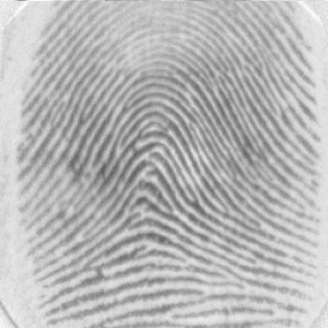
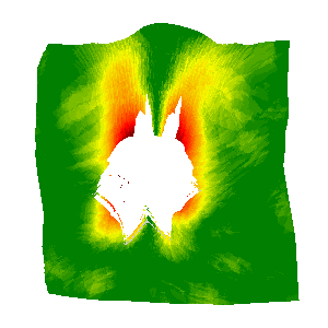
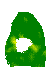
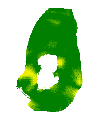
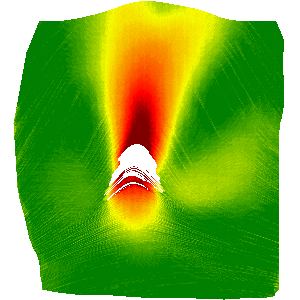
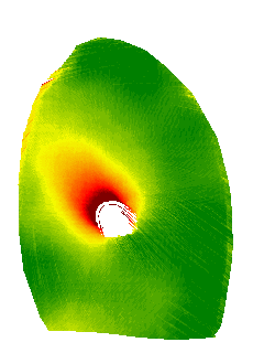
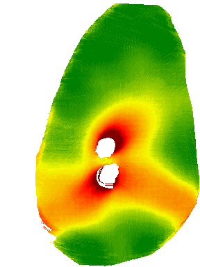
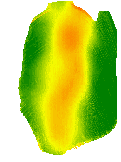
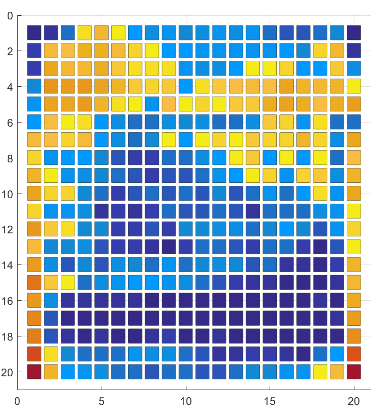
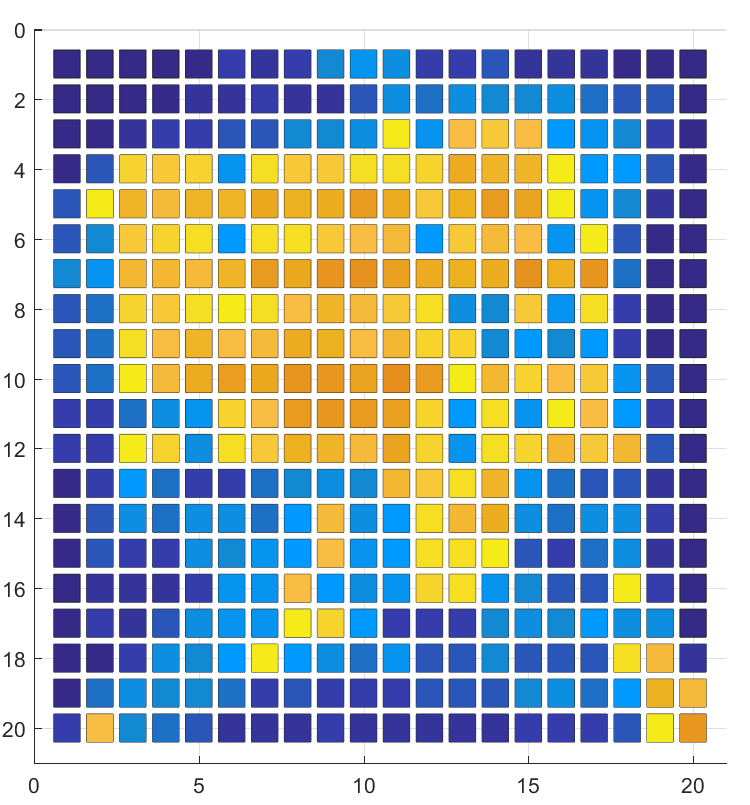
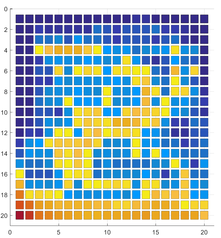
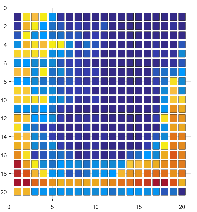
Figure 9: Exemplary fingerprints (top row) with conformality index field (2nd row), curvature field (3rd row) and joint histograms (bottom row, axes as in Fig, 8). The left three column are from real fingers, the right three columns from synthetic prints.

Considering the results for 20 bins per dimension and histograms based on one impression in Table 1, we observe classification accuracies on the training set of 100% and accuracies on the test set between 74 and 80%. We believe that the limiting factor for the accuracy is the very small number of training examples (60 real and 60 synthetic images) which could be resolved by larger databases.

Interestingly, histograms which summarize eight instead of just one impression achieve a perfect classification accuracy on both training and test set despite the small number of training examples. Computing an average histogram which captures the average joint distribution of curvature and Möbius moduli over several (eight) impressions seems to be robust under fluctuations in histograms between different impressions of the same finger.

In conclusion we remark that new algorithms for generating realistic synthetic orientation fields have to be developed. The recently proposed XQD model Gottschlich et al. (2017) could be used for this purpose, realistically linking curvature with conformality indeces. Until their arrival, one may rely on orientation fields from real fingerprints (as implemented by RFC Imdahl et al. (2015)).

References

- Ahlfors (1966) Ahlfors, L. (1966). Complex analysis: an introduction to the theory of analytic functions of one complex variable. McGraw Hill.
- Araque et al. (2002) Araque, J., M. Baena, B. Chalela, D. Navarro, and P. Vizcaya (2002). Synthesis of fingerprint images. In Proc. ICPR, pp. 422–425.
- Bartůněk et al. (2013) Bartůněk, J., M. Nilsson, B. Sällberg, and I. Claesson (2013, February). Adaptive fingerprint image enhancement with emphasis on preprocessing of data. IEEE Transactions on Image Processing 22(2), 644–656.
- Cappelli et al. (2000) Cappelli, R., A. Erol, D. Maio, and D. Maltoni (2000, September). Synthetic fingerprint-image generation. In Proc. ICPR, Barcelona, Spain, pp. 3–7.
- Chang and Lin (2011) Chang, C.-C. and C.-J. Lin (2011, April). LIBSVM : a library for support vector machines. ACM Transactions on Intelligent Systems and Technology 2(3), 1–27.
- Galar et al. (2015a) Galar, M. et al. (2015a, June). A survey of fingerprint classification part I: Taxonomies on feature extraction methods and learning models. Knowledge-Based Systems 81, 76–97.
- Galar et al. (2015b) Galar, M. et al. (2015b, June). A survey of fingerprint classification part II: Experimental analysis and ensemble proposal. Knowledge-Based Systems 81, 98–116.
- Gottschlich (2012) Gottschlich, C. (2012, April). Curved-region-based ridge frequency estimation and curved Gabor filters for fingerprint image enhancement. IEEE Transactions on Image Processing 21(4), 2220–2227.
- Gottschlich (2016) Gottschlich, C. (2016, February). Convolution comparison pattern: An efficient local image descriptor for fingerprint liveness detection. PLoS ONE 11(2), e0148552.
- Gottschlich and Huckemann (2014) Gottschlich, C. and S. Huckemann (2014, December). Separating the real from the synthetic: Minutiae histograms as fingerprints of fingerprints. IET Biometrics 3(4), 291–301.
- Gottschlich et al. (2009) Gottschlich, C., P. Mihăilescu, and A. Munk (2009, December). Robust orientation field estimation and extrapolation using semilocal line sensors. IEEE Transactions on Information Forensics and Security 4(4), 802–811.
- Gottschlich and Schönlieb (2012) Gottschlich, C. and C.-B. Schönlieb (2012, June). Oriented diffusion filtering for enhancing low-quality fingerprint images. IET Biometrics 1(2), 105–113.
- Gottschlich and Schuhmacher (2014) Gottschlich, C. and D. Schuhmacher (2014, October). The shortlist method for fast computation of the Earth Mover’s Distance and finding optimal solutions to transportation problems. PLoS ONE 9(10), e110214.
- Gottschlich et al. (2017) Gottschlich, C., B. Tams, and S. Huckemann (2017, May). Perfect fingerprint orientation fields by locally adaptive global models. IET Biometrics 6(3), 183–190.
- Huckemann et al. (2008) Huckemann, S., T. Hotz, and A. Munk (2008, September). Global models for the orientation field of fingerprints: an approach based on quadratic differentials. IEEE Transactions on Pattern Analysis and Machine Intelligence 30(9), 1507–1517.
- Imdahl et al. (2015) Imdahl, C., S. Huckemann, and C. Gottschlich (2015, September). Towards generating realistic synthetic fingerprint images. In Proc. ISPA, Zagreb, Croatia, pp. 78–82.
- Kücken and Champod (2013) Kücken, M. and C. Champod (2013). Merkel cells and the individuality of friction ridge skin. Journal of Theoretical Biology 317, 229–237.
- Maltoni et al. (2009) Maltoni, D., D. Maio, A. Jain, and S. Prabhakar (2009). Handbook of fingerprint recognition. Springer.
- Sherlock and Monro (1993) Sherlock, B. and D. Monro (1993). A model for interpreting fingerprint topology. Pattern recognition 26(7), 1047–1055.
- Strebel (1984) Strebel, K. (1984). Quadratic differentials. Springer.
- Thai and Gottschlich (2016) Thai, D. and C. Gottschlich (2016, June). Global variational method for fingerprint segmentation by three-part decomposition. IET Biometrics 5(2), 120–130.
- Thai et al. (2016) Thai, D., S. Huckemann, and C. Gottschlich (2016, May). Filter design and performance evaluation for fingerprint image segmentation. PLoS ONE 11(5), e0154160.
- Trefethen (2002) Trefethen, T. D. L. (2002). Schwarz-Christoffel Mapping, Volume 8. Cambridge University Press.
- Vizcaya and Gerhardt (1996) Vizcaya, P. and L. Gerhardt (1996). A nonlinear orientation model for global description of fingerprints. Pattern Recognition 29(7), 1221–1231.