T-Crowd: Effective Crowdsourcing for Tabular Data

Abstract

Crowdsourcing employs human workers to solve computer-hard problems, such as data cleaning, entity resolution, and sentiment analysis. When crowdsourcing tabular data, e.g., the attribute values of an entity set, a worker’s answers on the different attributes (e.g., the nationality and age of a celebrity star) are often treated independently. This assumption is not always true and can lead to suboptimal crowdsourcing performance. In this paper, we present the T-Crowd system, which takes into consideration the intricate relationships among tasks, in order to converge faster to their true values. Particularly, T-Crowd integrates each worker’s answers on different attributes to effectively learn his/her trustworthiness and the true data values. The attribute relationship information is also used to guide task allocation to workers. Finally, T-Crowd seamlessly supports categorical and continuous attributes, which are the two main datatypes found in typical databases. Our extensive experiments on real and synthetic datasets show that T-Crowd outperforms state-of-the-art methods in terms of truth inference and reducing the cost of crowdsourcing.

1 Introduction

Crowdsourcing is an effective way to address computer-hard problems (e.g., entity resolution [32, 31, 8] and sentiment analysis [39, 20]) by utilizing numerous ordinary humans (called workers or the crowd). The general workflow of crowdsourcing is as follows: at first a requester proposes a problem, then the problem is transformed into many tasks (i.e., questions), and finally the workers complete the tasks assigned to them and they are given a monetary reward.

Many applications[14, 25, 26] crowdsource tabular data, i.e., a collection of discrete and related items which are structured in a tabular form and comply to a schema. Each column represents a particular attribute or variable. Each row corresponds to an entity and includes a value for each of the variables. Table 1 illustrates an image recognition example; given the picture of a celebrity, the goal is to collect the name, nationality, age, and height of the person from the crowd. The values shown in Table 1 are the unknown (ground) truth data to be collected from the workers. Each cell of this table can be considered as a task, i.e., a worker may be asked to provide a value for the name of a celebrity given his/her picture [26].

Table 1: Ground Truth about Celebrities

	Picture	Name	Nationality	Age	Height
1		Gwyneth Paltrow	United States	40	5′9
2		Jet Li	China	45	5′6
3		James Purefoy	Great Britain	48	6′1

Table 2: Answers to Tasks about Celebrities

Worker	Pic Id	Name	Nationality	Age	Height
$u_{1}$	1	Gwyneth Paltrow	United States	39	5′9
	2	Jet Li	China	47	5′6
$u_{2}$	1	Gwyneth Paltrow	Canada	45	5′11
	3	James Purefoy	Great Britain	51	6′
$u_{3}$	2	Jet Li	China	45	5′6
	3	Ciarán Hinds	United States	35	5′11

Crowdsourcing involves two interrelated processes: truth inference and task assignment. Truth inference refers to addressing noise and errors from the crowd in order to eventually infer the correct answer (or truth) for each task based on the answers to it by all workers [11, 34]. Existing works [10, 33, 37, 40] often model that a worker’s quality is consistent in all the tasks. Task assignment refers to selecting an appropriate set of tasks to assign to each incoming worker. Selection of a task to assign can be based on how confident we are already about the true value of the task (i.e., whether we need more answers) [5] and/or what is the estimated quality (i.e., reliability) of the worker on the specific task (i.e., the expected information gain after the corresponding assignment) [39, 16]. Truth inference can be used as a module in task assignment, to estimate the confidence of estimated true values [5, 20].

Most crowdsourcing systems assume that the set of crowdsourced tasks are homogeneous and independent to each other. For example, consider an image tagging problem; all tasks request the same type of input from the workers (i.e., a set of keywords) and there are no obvious dependencies among different images. In this paper, we focus on crowdsourcing tabular data, which are directly related to database applications. We identify the properties of these data that make the application of previous work challenging and create opportunities for more effective crowdsourcing.

First, the datatypes and domains of different attributes may vary. For example, in Table 1, the task “What is the nationality of the person in Picture 1?” has a different datatype compared to the task “What is the height of the person in Picture 2?” (i.e., categorical vs. continuous). Even attributes of the same datatype may have different domains. As a result, approaches for integrating the answers of a worker in homogeneous tasks in order to estimate the worker’s quality are not directly applicable. These include the popular EM algorithm [9] for categorical data and data integration models applied for continuous attributes (GTM [37] and CATD [17]), to be discussed in Section 2. As we will show, applying a different approach for each column does not transfer the knowledge from one datatype to the other, i.e., the estimation of worker quality can be inaccurate due to data sparsity.

Second, in tabular data, there are potential dependencies between rows and columns. The difficulty of a task might depend on the corresponding entity and attribute. As a result, the quality of a worker on a particular task may depend on his/her quality on other tasks in the same row or column. Take Table 2 as an example, which contains the answers of three workers on tasks from Table 1. Observe that worker $u_{3}$ inputs a wrong name for the third picture, which means that he does not recognize this celebrity. If we allow him to provide values for the nationality, age and height of the person in that picture, his answers would be unreliable, despite the high quality of his input for the second picture. This means that when computing the quality of a worker for truth inference or task assignment, we should not consider the columns independently, but we should take such possible dependencies under consideration.

In this paper, we present the T-Crowd system, the first crowdsourcing solution that considers all the aforementioned properties of tabular data in both truth inference and task assignment. T-Crowd processes the submitted answers by each worker to infer a single quality for him or her, based on the assumption that the quality of each worker is consistent throughout the entire table. T-Crowd seamlessly integrates the worker’s answers to tasks of different datatypes and domains, addressing consistency and data sparsity issues that would arise from the alternative approach of using different models for different columns. For example, the overall quality of worker $u_{1}$ can be regarded as better than that of worker $u_{2}$ considering their answers to both categorical and continuous values in Table 2. Unified worker quality greatly improves the accuracy of truth inference and the performance of task assignment, reducing the total number of tasks to be assigned to workers until all true values are estimated with high confidence.

T-Crowd includes a model that captures the importance of tasks (i.e., how confident we are about their value estimates) in the different columns and rows, based on the collected data so far. We also consider the quality of the worker who is answering and define an inherent information gain which is a uniform measure for ranking tasks with respect to a given worker. Then we choose to assign to the worker the tasks with the highest anticipated benefit. In contrast, previous work on crowdsourcing tabular data performs task assignment based on only how many more answers are needed for each task, disregarding worker quality. To further improve performance, we utilize the potential correlations between tasks. We define a structure-aware information gain which extends the inherent information gain to also consider as a parameter the previous answers given by the worker on tasks that appear in the same row, when selecting new tasks to assign to him or her.

To summarize, our main contributions are as follows:

• We unify worker quality for all tasks in crowdsourced tabular data, improving the accuracy of truth inference and the performance of task assignment, compared to models that treat each attribute independently.

• Given an incoming worker, we find a suitable set of tasks for him/her based on the benefit of obtaining additional answers in tasks, the worker’s inherent quality, and the correlation of answer quality between tasks in the same row.

• We evaluate T-Crowd on real and synthetic datasets; the results demonstrate its superiority over existing alternatives. Compared to previous work, T-Crowd has better truth inference accuracy and converges to the true values of the tasks using only about half of the answers by the workers.

The rest of the paper is organized as follows. Section 2 discusses related work. Section 3 defines the problem and gives an overview of our system. In Section 4, we present our methodology for truth inference. Our task assignment policy is presented in Section 5. Section 6 includes our experimental evaluation. Finally, we conclude in Section 7.

2 related work

Related work falls into two categories: truth inference methods used to infer the truth and task assignment strategies for a incoming worker.

Truth Inference. The most basic truth inference methods are majority voting for multiple-choice tasks (i.e., categorical data) and taking the median for numerical tasks (i.e., continuous data). These approaches regard all workers as equal, disregarding any differences in their trustworthiness. Methods such as D$\&$S [9, 15] use a confusion matrix to model a worker’s quality of a worker, and then use an Expectation-Maximization (EM) algorithm to infer the truth. More advanced approaches like TruthFinder [35], Accusim [12], and GLAD [33] improve accuracy using different worker answering models or by considering more parameters, such as the difficulty of the task. These methods focus on answering tasks on categorical data. Other methods, such as GTM [37], are designed for continuous crowdsourced data. CRH [18, 19] and CATD [17] are two existing truth inference approaches for both categorical and continuous data. CRH [18] incorporates different distance functions between the answers and the estimated truth to recognize the characteristics of various data types. Specifically, CRH proposes an objective function and minimizes it by updating the estimated true values and source reliability (i.e., worker quality) in turns. CATD [17] considers both source reliability and the confidence interval of the estimation. Additional information of tasks or workers has also been considered in truth inference, such as the latent topics of the tasks [21] and the learn bias of workers [41].

The aforementioned works do not take into account the nature of tabular data that we address in this paper. In Section 4, we present an iterative Expectation-Maximization (EM) truth inference algorithm, which improves the accuracy of truth inference from the answers compared to previous work. The novelty of our work is that we use a probabilistic model for the answers of workers for different data types and that we unify workers’ quality on categorical data and continuous data explicitly, while methods like CRH design different distance functions for the different data types. As CRH is primarily designed to discover truth from web data, it may not adapt well to the problem of inferring truths from workers’ answers, which exhibit a long-tail distribution. Our approach, which is customized for crowdsourcing, performs better than CRH experimentally.

Task Assignment. Online task assignment selects which tasks to assign to each incoming worker, in order to achieve the maximum possible quality for the collected data. In simple crowdsourcing systems, like CDAS [20], the candidate tasks are randomly assigned to workers. AskIt [5] is yet another crowdsourcing platform, which assigns the tasks that have the highest uncertainty, again disregarding the quality (or expertise) of the incoming worker for these tasks. CrowdDB [14], Deco [25], and Qurk [22] are extensions of relational database systems that incorporate the crowd’s knowledge into query processing. They use answers from the crowd to make up the missing values of query operators. They are similar to our approach in that they collect tabular data; however, they do not focus on the assignment strategy and simply assign random tasks to workers. CrowdFill [26] is the most similar and recent system for tabular data. In CrowdFill, the workers are asked to select and answer tasks from a subset of the table given to them and they can also vote for the answers to these tasks by other workers. Due to the different way of acquiring data from workers, CrowdFill is not directly comparable to our work. Besides, CrowdFill does not estimate worker quality, and does not use properties of tabular data (e.g., attribute dependencies) to assign tasks to workers. Some methods [13, 38, 23] consider the case where the tasks are relevant to different domains and workers are given the tasks that match their domain expertise. In [7, 36], task assignment is modeled by a Markov Decision process and solved as a multi-armed bandit problem, but the application of the model is limited to only single-choice or multiple-choice tasks. Other forms of online task assignment, which need explicit workers’ collaboration, have been studied in [28, 29].

Different from the above works, our method focuses on crowdsourcing datasets, which are structured and heterogeneous, presenting challenges and opportunities as discussed in the Introduction. We consider the currently collected data, the difficulty of tasks, and the correlations of answer quality for tasks that refer to the same entity, to estimate the quality of workers and to conduct task assignment targeting the maximization of information gain of tasks.

Table 3: Table of Notations

Notation	Description
$c_{ij}$	cell (task) in the $i$-th row and $j$-th column
$a_{ij}^{u}$	answer given by worker $u$ for cell $c_{ij}$
$\mathcal{A}$	the set of all answers, i.e., $\mathcal{A}=\{a_{ij}^{u}\}$
$T_{ij}$	distribution of estimated truth for cell $c_{ij}$
$T_{ij}^{*}\leavevmode\nobreak\ (\widehat{T}_{ij})$	ground truth (estimated truth) for cell $c_{ij}$
$e_{ij}^{u}$	error of $a_{ij}^{u}$ with respect to $\widehat{T}_{ij}$
$q_{u}$	quality of worker $u$
$\alpha_{i}\leavevmode\nobreak\ (\beta_{j})$	difficulty of row $i$ (column $j$)

3 Problem Definition

In this section, we formulate the problem and give an overview of T-Crowd. As discussed in Section 1, our goal is to perform crowdsourcing on a two-dimensional table $C$, defined as follows.

Definition 1 (Tabular Data Model)

We target the crowdsourcing of a two-dimensional table $C=\{c_{ij}\}$, where $i\in\{1,...,N\}$ and $j\in\{1,...,M\}$. $C$ has an entity attribute which is the key attribute of the table. Each column is a categorical or a continuous attribute. Each cell $c_{ij}$ represents the value of the $i$-th entity in the $j$-th attribute, whose true value (i.e., truth, or ground truth) is denoted as $T_{ij}^{*}$.

Table 1 shows an example of tabular data about celebrities that we want to crowdsource. Age and Height are continuous attributes, while Name and Nationality are categorical attributes. The entity attribute is Picture. To obtain the truth for the remaining attributes, we ask the crowd to provide answers.

Definition 2 (Task, Worker, Answer)

A task is
related to a cell $c_{ij}$ and the crowd (or workers) is asked to answer the task, by providing values for the cell. Let $U$ be a set of workers. A worker $u\in U$ will submit an answer $a_{ij}^{u}$, if cell $c_{ij}$ is assigned to $u$.

For example, to get the age of the second entity, a task provides the picture of the second entity and asks workers to input the age. Since workers may have different levels of quality (e.g., some workers are experts, while some are spammers), each task $c_{ij}$ is often assigned to multiple workers and all acquired answers for $c_{ij}$ are aggregated to infer the true value of $c_{ij}$. Next, we define the two problems that we are addressing in this paper.

Definition 3 (Truth Inference)

Given the set of
answers $\{a_{ij}^{u}\}$, by workers $u\in U$ to cells $c_{ij}$, $i\in\{1,...,N\}$, $j\in\{1,...,M\}$, the problem of truth inference is to compute an accurate estimate $\widehat{T}_{ij}$ for each cell $c_{ij}$’s true value $T_{ij}^{*}$.

Definition 4 (Task Assignment)

When a worker $u$ requests for a task for $C$, decide the task to be assigned to $u$.

As we will discuss, a worker’s previous answers, as well as other workers’ answers, are both instrumental in task assignment. It is also worth to note that existing crowdsourcing platforms, such as the Amazon Mechanical Turk (AMT) [1], support the functionality of dynamically assigning tasks to an incoming worker (e.g., the ‘external-HIT’ feature in AMT [2]). Table 3 summarizes the notations used in this paper.

System architecture. Figure 1 gives an overview of T-Crowd, our proposed system for crowdsourcing tabular data. A requester (e.g., a lifestyle journal) first defines the structure (i.e., schema) of the collected data, such as the datatypes of the columns, and the key attribute. Then the requester publishes tasks to a crowdsourcing platform, e.g., AMT [1]. For an incoming worker $u$, our Task Assignment module determines one or more cells and assigns the corresponding task(s) to $u$. This is based on the anticipated information gain of the different cells by $u$’s answers. Intuitively, the information gain is an estimate of how much more accurate the cells’ values become upon collection of $u$’s inputs. When the worker submits an answer $a_{ij}^{u}$ for a cell $c_{ij}$ to the system, the Truth Inference module infers the estimated truth $\widehat{T}_{ij}$. To facilitate task assignment and truth inference, we also estimate the quality of worker $q_{u}$ and the difficulty of cells $\alpha_{i}$ and $\beta_{j}$. It assigns task(s) to workers and collect answers from workers before the budget is exhausted.

Figure 1: System Architecture

4 Truth Inference

In this section, we explain how T-Crowd performs truth inference on tabular data. The quality of truth inference for a data cell $c_{ij}$ depends on the quality of workers who answer $c_{ij}$, and the difficulty of $c_{ij}$. We first discuss how to model worker quality and cell difficulty (Sections 4.1 and 4.2). Then, we show how to infer the true values of cells based on these two factors (Section 4.3).

4.1 Quality of a Worker

The challenge in modeling worker quality is that attributes may have different datatypes and difficulties; the answer set of a categorical task is finite and nominal, while that of a continuous task is an integer or a real number. Hence, it is not straightforward to model the quality of a worker using a single parameter. To address this problem, we propose a unified model for both categorical and continuous attributes.

We model the truth of a categorical attribute $l^{*}$ as an element in a finite unordered set of possible answers $L=\{l_{1},l_{2},...,l_{|L|}\}$. An answer from a worker is either correct or wrong depending on whether it is the same as the ground truth. On the other hand, for a continuous attribute, the quality of the answer depends on how close it is to the ground truth. For example, if the height of Jet Li is 5^′6, and a worker answers 5^′7, which is close to the truth, the answer is considered to be a good one.

As discussed, our goal is to use a single parameter $q_{u}$ to represent the quality of a worker $u$. For the ease of presentation, we first illustrate how the worker’s quality for continuous datatypes can be modeled, and then show how the model can be extended for categorical datatypes.

$\bullet$ For continuous datatypes, we model the distribution of the answer given by worker $u$ as a normal distribution: $a_{ij}^{u}\sim\mathcal{N}(\widehat{T}_{ij},\phi_{u})$:

$$\vspace{-.5em}P(a_{ij}^{u}=x)=\frac{1}{\sqrt{2\pi\phi_{u}}}\,\exp\big{(}{-\frac{(x-\widehat{T}_{ij})^{2}}{2\phi_{u}}}\big{)},$$ (1)

where $\widehat{T}_{ij}$ is the expected value of $c_{ij}$ and $\phi_{u}$ is the variance of $u$. Intuitively, the higher the quality of a worker is, the smaller the variance will be, as her answer should have smaller difference from the truth. Inspired by this, we model $q_{u}\in[0,1]$ as the probability that the answer from worker $u$ falls into a small range ($\epsilon$) around the truth $\widehat{T}_{ij}$:

$$q_{u}=P(\leavevmode\nobreak\ a_{ij}^{u}\in[\widehat{T}_{ij}-\epsilon,\widehat{T}_{ij}+\epsilon]\leavevmode\nobreak\ )=\text{erf}({\epsilon}/{\sqrt{2\phi_{u}}}).$$ (2)

Intuitively, $q_{u}$ is the area under the normal distribution curve, where $\epsilon$ is a general parameter that controls the shape of the area and “erf” is the Gauss error function [4].

$\bullet$ For categorical attributes, $q_{u}\in[0,1]$ indicates the probability that the worker $u$ would correctly answer a task, i.e.,

$$P(a_{ij}^{u}=z)=(q_{u})^{\mathds{1}_{\{\widehat{T}_{ij}=z\}}}\cdot\big{(}\frac{1-q_{u}}{|L|-1}\big{)}^{\mathds{1}_{\{\widehat{T}_{ij}\neq z\}}},$$ (3)

where $\mathds{1}_{\{\cdot\}}$ is an indicator function which returns 1 if the argument is true; 0, otherwise. For example, $\mathds{1}_{\{5=5\}}=1$ and $\mathds{1}_{\{5=3\}}=0$. Intuitively, worker $u$ has probability $q_{u}$ to give the correct answer and we evenly distribute the probability $(1-q_{u})$ to the remaining (false) answers. Note that $q_{u}$ can be expressed as in Eq. 2, meaning that we can use the same quality measure for categorical and continuous attributes.

4.2 Difficulty of a Cell

The answers from workers do not only depend on their expertise, but they are also influenced by the difficulty of tasks. Hence, in our model, the quality of answer $a_{ij}^{u}$ depends on the quality of worker $u$, the difficulty $\beta_{j}$ of attribute (i.e., column) $j$, and the difficulty $\alpha_{i}$ of entity (i.e., row) $i$.

To incorporate the difficulty of each cell $c_{ij}$ into the worker’s quality, we define the variance of his/her answer to a cell $c_{ij}$ as $\phi^{u}_{ij}=\alpha_{i}\beta_{j}\phi_{u}$. This means that the variance is positively correlated to the difficulties $\alpha_{i}$ and $\beta_{j}$, and the inherent variance ($\phi_{u}$) of answers by worker $u$. Then, following Equation 2, we represent the quality of worker $u$ answering cell $c_{ij}$ as $q^{u}_{ij}=\text{erf}\left(\epsilon/\sqrt{2\alpha_{i}\beta_{j}\phi_{u}}\right)$. To model the worker’s answers on categorical and continuous data, Equations 1 and 3 can be changed accordingly, i.e., by replacing $\phi_{u}$ with $\phi^{u}_{ij}$ and $q_{u}$ with $q^{u}_{ij}$.

Note that $\widehat{T}_{ij}$, $\alpha_{i}$, $\beta_{j}$ and $\phi_{u}$ are unknown and we discuss how to compute them later. The worker quality $q_{u}$ ($q_{ij}^{u}$) can be calculated directly if we know $\alpha_{i}$, $\beta_{j}$, and $\phi_{u}$.

4.3 Inference Process

The objective function of the truth inference problem is to maximize the likelihood of workers’ answers, i.e.,

$$\arg\max_{\alpha,\beta,\phi}P(\mathcal{A}|\alpha,\beta,\phi)=\arg\max_{\alpha,\beta,\phi}\sum\nolimits_{\mathcal{T}}P(\mathcal{A},\mathcal{T}|\alpha,\beta,\phi),$$

where $\mathcal{A}$ is the current set of answers by all workers on all cells and $\mathcal{T}$ is a set of all hidden true values, i.e., $\mathcal{T}=\{T_{ij}\}$. $T_{ij}$ denotes the estimated distribution of truth in cell $c_{ij}$. To optimize this non-convex function, we use the Expectation-Maximization (EM) algorithm [11], which takes an iterative approach. In each iteration of EM, the E-step computes the hidden variables in $\mathcal{T}$, and the M-step computes the parameters $\alpha_{i}$, $\beta_{j}$ and $\phi_{u}$ ($q_{u}$). Next, we provide details about the E-step and the M-step.

Expectation Step (E-step). In the E-step, we compute the posterior probabilities of hidden variable $T_{ij}\in\mathcal{T}$ given the values of $\alpha$, $\beta$ and $\phi$ and the observed variable $A_{ij}=\{a_{ij}^{u}\},u\in U_{ij}$, i.e., the current answer set of cell $c_{ij}$.

$$\begin{split}&P(\leavevmode\nobreak\ T_{ij}=z|A_{ij},\alpha_{i},\beta_{j},\phi\leavevmode\nobreak\ )\propto\\ &\prod\nolimits_{u\in U_{ij}}P(a_{ij}^{u}|T_{ij}=z,\alpha_{i},\beta_{j},\phi_{u})\cdot\text{Prior}(T_{ij}=z).\end{split}$$ (4)

Based on our defined worker model of $P(T_{ij}=z|A_{ij},\alpha_{i},\beta_{j},\phi)$ for different datatypes, the distribution is defined as follows.
(1) For cells $c_{ij}$ of continuous type, we regard that $\text{Prior}(T_{ij}=z)$ follows a normal distribution $\mathcal{N}(\mu^{0}_{j},\leavevmode\nobreak\ \phi^{0}_{j})$, and $T_{ij}\sim$ $\mathcal{N}({T^{\mu}_{ij},\leavevmode\nobreak\ T^{\phi}_{ij}})$, where $T^{\mu}_{ij}$ and $T^{\phi}_{ij}$ satisfy that

$$T^{\mu}_{ij} =\big{(}\sum\nolimits_{u\in U_{ij}}\frac{a_{ij}^{u}}{\alpha_{i}\beta_{j}\phi_{u}}+\frac{\mu^{0}_{j}}{\phi^{0}_{j}}\big{)}\leavevmode\nobreak\ T^{\phi}_{ij},$$

$$T^{\phi}_{ij} =\big{(}\sum\nolimits_{u\in U_{ij}}\frac{1}{\alpha_{i}\beta_{j}\phi_{u}}+\frac{1}{\phi^{0}_{j}}\big{)}^{-1}.$$

(2) For cells $c_{ij}$ of categorical type, we have

$$P(T_{ij}=z)=\frac{\prod_{u\in U_{ij}}[(q^{u}_{ij})^{\mathds{1}_{\{a_{ij}^{u}=z\}}}(\frac{1-q^{u}_{ij}}{|L_{j}|-1})^{\mathds{1}_{\{a_{ij}^{u}\neq z\}}}]}{\sum_{z\in L_{j}}\prod_{u\in U_{ij}}[(q^{u}_{ij})^{\mathds{1}_{\{a_{ij}^{u}=z\}}}(\frac{1-q^{u}_{ij}}{|L_{j}|-1})^{\mathds{1}_{\{a_{ij}^{u}\neq z\}}}]},$$

where $q^{u}_{ij}$ is defined as $\text{erf}\left(\epsilon/\sqrt{2\alpha_{i}\beta_{j}\phi_{u}}\right)$ and $L_{j}$ is the label set of column $j$. $\text{Prior}(T_{ij}=z)$ is uniform so it disappears.

Intuitively, the answer given by high quality worker will be trusted more, i.e., given higher weight. To be specific, we estimate the truth distribution $T_{ij}$ by combining the set $A_{ij}$ of workers’ answers for $c_{ij}$. (1) $T^{\mu}_{ij}$ can be regarded as a weighted average of answer $a_{ij}^{u}$ based on the quality $\alpha_{i}\beta_{j}\phi_{u}$. $T^{\phi}_{ij}$ is a normalized term. (2) Similarly, $P(T_{ij}=z)$ is a normalized product of the qualities $q^{u}_{ij}$ of the workers whose answer $a_{ij}^{u}$ is $z$.

Maximization Step (M-step). In the M-step, we find the values of parameters $\alpha$, $\beta$ and $\phi$ that maximize the expectation of the joint log-likelihood of the observed variable $\mathcal{A}$, as shown below:

$$Q(\alpha,\beta,\phi)=\operatorname{E}_{\mathcal{T}}[\ln P(\mathcal{A},\mathcal{T}|\alpha,\beta,\phi)]$$ (5)

$$= \sum_{j}\sum_{i}\leavevmode\nobreak\ \operatorname{E}_{T_{ij}}\big{[}\ln\text{Prior}(T_{ij})+\sum_{u\in U_{ij}}\ln P(a_{ij}^{u}|T_{ij},\alpha_{i},\beta_{j},\phi_{u})\big{]}.$$

Formula $\operatorname{E}_{T_{ij}}[\sum_{u\in U_{ij}}\ln P(a_{ij}^{u}|T_{ij},\alpha_{i},\beta_{j},\phi_{u})]$ is calculated for the different datatypes, as follows.
(1) For cells $c_{ij}$ of continuous type:

$$\sum\nolimits_{u\in U_{ij}}[-\frac{1}{2}\ln(2\pi\alpha_{i}\beta_{j}\phi_{u})-\frac{({a_{ij}^{u}}-T_{ij}^{\mu})^{2}+T_{ij}^{\phi}}{2\alpha_{i}\beta_{j}\phi_{u}}].$$

(2) For cells $c_{ij}$ of categorical type:

$$\begin{split}\sum\nolimits_{z\in L_{j}}P(T_{ij}=z)\cdot\sum\nolimits_{u\in U_{ij}}\big{(}&{\mathds{1}_{\{a_{ij}^{u}=z\}}}\ln\text{erf}(\frac{\epsilon}{\sqrt{2\alpha_{i}\beta_{j}\phi_{u}}})\\ +&{\mathds{1}_{\{a_{ij}^{u}\neq z\}}}\ln\frac{1-\text{erf}(\frac{\epsilon}{\sqrt{2\alpha_{i}\beta_{j}\phi_{u}}})}{|L_{j}|-1}\big{)}.\end{split}$$

We apply gradient descent to find the values of $\alpha$, $\beta$ and $\phi$ that locally maximize $Q(\alpha,\beta,\phi)$.

Intuitively, a worker will be of high quality if his/her answers are close to the estimated truth. Thus, we compute a value $\phi_{u}$ that maximizes the expectation of the log-likelihood of worker $u$’s answers $a_{**}^{u}$. Similarly, we also find an $\alpha_{i}$ (resp. $\beta_{j}$) that maximizes the expectation of the log-likelihood of answers $a_{i*}^{*}$ in row $i$ (resp. $a_{*j}^{*}$ in column $j$).

Algorithm. By combining the two steps above, we can iteratively update the parameters until convergence. Each $T_{ij}$ is initialized by following the distribution in $\text{Prior}(T_{ij})$. At each iteration, the M-step applies gradient descent to find $\alpha_{i}$, $\beta_{j}$ and $\phi_{u}$ by maximizing Equation 5 and the E-step applies Equation 4. We identify convergence if the differences between the parameter values in subsequent iterations are below a threshold (e.g., $10^{-5}$).

Finally we estimate the truth $\widehat{T}_{ij}$ of each cell $c_{ij}$ as:

$$\widehat{T}_{ij}=\begin{cases}T^{\mu}_{ij}&,\leavevmode\nobreak\ c_{ij}\text{ is continuous},\\ \arg\max_{z\in{L_{j}}}\leavevmode\nobreak\ P(T_{ij}=z)&,\leavevmode\nobreak\ c_{ij}\text{ is categorical}.\end{cases}$$

Algorithm 1 shows the detailed process of inference.

Time Complexity. In the E-step, computing hidden variable $T_{ij}$ for a continuous cell $c_{ij}$ requires looping through the observed variable $A_{ij}=\{a_{ij}^{u}\}$, hence the complexity is $\mathcal{O}(|A_{ij}|)$. For a categorical cell $c_{ij}$, we need to additionally loop through the possible answers, thus the cost becomes $\mathcal{O}(l\cdot|A_{ij}|)$ where $l=\text{max}_{j}(|L_{j}|)$. The total cost of the E-step is therefore $\mathcal{O}(l\cdot|\mathcal{A}|)$, where $\mathcal{A}$ is the set of all obtained answers. In the M-step, to compute $Q(\alpha,\beta,\phi)$, we need to loop for each cell and workers who answered this cell. The number of loops is the same as $|\mathcal{A}|$. Since we use gradient descent, we need to also compute the gradient of each parameter which takes $\mathcal{O}(l\cdot|\mathcal{A}|)$. If gradient descent takes $v$ iterations to converge, this step takes $\mathcal{O}(vl\cdot|\mathcal{A}|)$ time in total. Assuming that the algorithm needs $w$ iterations to converge, the total time complexity is $\mathcal{O}(wvl\cdot|\mathcal{A}|)$. In practice, $l$ is constant, and $v$ and $w$ are smaller than 20, thus the time complexity is linear to the number of answers.

Input: workers’ answers $a_{ij}^{u}\in\mathcal{A}$, prior distribution of truth $\text{Prior}(T_{ij})$

Output: truth distribution $T_{ij}\in\mathcal{T}$, worker’s quality $\phi_{u}$, difficulty of row $\alpha_{i}$ and column $\beta_{j}$

1

2Initialize $T_{ij}$ using $\text{Prior}(T_{ij})$

3 while  true  do

4      

5       // Step 1: Estimate Worker Quality and Cell Difficulty

6       Compute $\alpha_{i}$, $\beta_{j}$ and $\phi_{u}$ maximizing Eq. 5;

7       // Step 2: Infer the Truth

8       for $1\leq i\leq N$ do

9             for $1\leq j\leq M$ do

10                   Obtain $T_{ij}$ by Eq. 4;

11                  

12            

13       // Check for Convergence

14       if Converged then

15            break;

16      

17return $T_{ij}$, $\alpha_{i}$, $\beta_{j}$ and $\phi_{u}$;

18

Algorithm 1 Truth Inference Method

5 Online Task Assignment

In this section, we discuss how we select tasks for a worker $u$. Section 5.1 defines an inherent information gain function to measure the utility of assigning a task to the worker, which can handle both categorical and continuous data. The function considers the quality of the worker, the need to obtain more answers for the task, and the task’s difficulty. Intuitively, we prefer to assign tasks whose gain of information will be improved the most if the incoming worker answers them. In Section 5.2, we extend this to a structure-aware information gain function, which also considers the correlations in the qualities of answers given by the same worker to different cells of the same row. Section 5.3 discusses the assignment of multiple tasks to $u$.

5.1 Inherent Information Gain

We need a uniform measure for the utility (or benefit) of assigning a task (either categorical or continuous) to a worker $u$ with quality $q_{u}$. For this purpose we define an inherent information gain function, following the steps below.

(1) For a categorical cell $c_{ij}$, the distribution of truth $T_{ij}$ has been computed by $P(T_{ij}=z)$ in Equation 4, which is the probability that label $z$ is correct. Thus, Shannon Entropy [3], a well-studied measure, can be used to define the uncertainty of task $c_{ij}$:

$$H_{s}(T_{ij})=-\sum\nolimits_{z\in L_{j}}P(T_{ij}=z)\ln{P(T_{ij}=z)}.$$

(2) For a continuous cell $c_{ij}$, note that for a continuous distribution, the Differential Entropy [24] is defined as:

$$-\int_{\mathbb{X}}f(x)\ln f(x)\,dx,$$

where $f(x)$ is a probability distribution. Recall that we also define the distribution of truth $T_{ij}\sim\mathcal{N}(T_{ij}^{\mu},T_{ij}^{\phi})$ of a continuous cell $c_{ij}$ in Equation 4, so its Differential Entropy can be computed as:

$$H_{d}(T_{ij})=\frac{1}{2}\,{\ln{\left(2\,\pi\,e\,T^{\phi}_{ij}\right)}}.$$

Given the above, we define a uniform entropy for a task $c_{ij}$ as:

$$H(T_{ij})=\begin{cases}H_{d}(T_{ij}),&\leavevmode\nobreak\ \text{if }c_{ij}\text{ is continuous},\\ H_{s}(T_{ij}),&\leavevmode\nobreak\ \text{if }c_{ij}\text{ is categorical}.\end{cases}$$

A straightforward approach for task assignment to a worker $u$ is to select the task $c_{ij}$ with the largest uniform entropy. However, this is problematic, as Differential Entropy and Shannon Entropy are not comparable; hence, task assignments may be biased toward one datatype. For example, as pointed out in [24], Differential Entropy can be negative while Shannon entropy is always non-negative.

Alternatively, we use Delta Entropy to measure the information gain. Suppose $\mathcal{A}_{C}$ is the current set of answers we have collected, we can obtain the estimated truth distribution (denoted as $T_{ij,\mathcal{A}_{C}}$) for each task $c_{ij}$ by the truth inference method presented in Section 4. Specifically, for an incoming worker $u$, we define the inherent information gain of assigning task $c_{ij}$ to her as:

$$IG_{q}(c_{ij})=H(T_{ij,\mathcal{A}_{C}})-\operatorname{E}_{a_{ij}^{u}}[H(T_{ij,\mathcal{A}_{C}\cup\{a^{u}_{ij}\}})],$$ (6)

where $T_{ij,\mathcal{A}_{C}\cup\{a^{u}_{ij}\}}$ is the updated distribution of the estimated truth for task $c_{ij}$ after receiving a new answer $a_{ij}^{u}$ from worker $u$.

By using the inherent information gain measure defined in Equation 6, we alleviate the problem that the domains of the two entropy types are different. If we discretize the range of a continuous random variable $X$ using bins of width $\Delta$, we can compute the Shannon entropy for this new discretized random variable $X^{\Delta}$, and we have the following formula if $X$’s pdf is Riemann integrable:

$$H_{s}(X^{\Delta})+\ln\Delta\to H_{d}(X),\leavevmode\nobreak\ as\leavevmode\nobreak\ \Delta\to 0.$$

Hence, if $\Delta$ is small, $H_{d}(X_{1})-H_{d}(X_{2})\approx H_{s}(X_{1}^{\Delta})-H_{s}(X_{2}^{\Delta})$, which means that the subtraction of differential entropies can be transformed into subtraction of Shannon entropies. As a result, for cells of different types, $IG(c_{ij})$ is comparable. Algorithm 2 shows the detailed process of assignment.

Computing the distribution of $\operatorname{E}_{a_{ij}^{u}}[H(T_{ij,\mathcal{A}_{C}\cup\{a^{u}_{ij}\}})]$. The distribution of an answer $a_{ij}^{u}$ follows the worker model in Equations 1 and 3 for continuous and categorical tasks, respectively. For a categorical task $c_{ij}$, the domain of $a_{ij}^{u}$ is a finite label set, so we use all possible values $a_{ij}^{u}$ to obtain $T_{ij,\mathcal{A}_{C}\cup\{a_{ij}^{u}\}}$ using the inference method described in Section 4. For a continuous task, since the the domain of $a_{ij}^{u}$ is $\mathcal{R}$, we apply sampling to approximate the value of $T_{ij,\mathcal{A}_{C}\cup\{a_{ij}^{u}\}}$. However, it is quite expensive to run the inference method for each possible answer. Because one more possible answer is quiet small compared with current set of answers, we accelerate by updating the parameters related to this answer mostly and maintaining other parameters. Thus, for a new answer $a_{ij}^{u}$, we update truth distribution $T_{ij}$, and the qualities of workers who have answered task $c_{ij}$.

Time Complexity. To compute the benefit for each task $c_{ij}$ (Equation 6), we should first iterate through the possible answers given by the incoming worker and compute a new distribution of truth $T_{ij}$. The number of possible answers for a categorical task $c_{ij}$ is $|L_{j}|$ and for a continuous task is the fixed sampling number $s_{\text{cont}}$. Because we approximate the inference method, it only takes $\mathcal{O}(l\cdot|P|)$ where $P$ is the set of parameters we need to update. Let $s=\text{max}(\text{max}_{j}(|L_{j}|),s_{\text{cont}})$; the total cost of considering one task for a certain worker is $\mathcal{O}(sl\cdot|P|)$. Then, computing the information gains of all tasks takes $\mathcal{O}(NMsl\cdot|P|)$. Since $P$ includes the truth distribution $T_{ij}$ and the qualities of workers who have answered task $c_{ij}$, $P$ mainly depends on the average answers per task. Thus, $\mathcal{O}(NMsl\cdot|P|)\approx\mathcal{O}(sl\cdot|\mathcal{A}|)$.

Parallel or distributed computation can be used to accelerate task assignment, as the consideration of the different tasks are independent. For example, we separate different tasks and different possible answers to different machines or processes and compute the corresponding information gains in parallel without the need of data communication.

Input: Budget $B$

Output: truth distribution $T_{ij}\in\mathcal{T}$

1

2Initialize each task with several answers from workers

3

4while  Budget $B$ is not exhausted  do

5      

6       // Step 1: Analyze current situation

7       Run truth inference to obtain $T_{ij}$, $\alpha_{i}$, $\beta_{j}$ and $\phi_{u}$

8       // Step 2: Find task $c^{*}$ with highest benefit for incoming worker $u$

9      

10      for $1\leq i\leq N$ do

11             for $1\leq j\leq M$ do

12                   Compute information gain $IG(c_{ij})$ by Eq.6

13                   if $IG(c_{ij})>IG(c^{*})$ or $c^{*}$ is not defined then

14                        $c^{*}=c_{ij}$

15                  

16            

17      

18       // Step 3: Collect answers

19       Publish task $c^{*}$ and collect worker $u$’s answer

20

21Run truth inference to obtain the final $T_{ij}$

22 return $T_{ij}$

23

Algorithm 2 Online Task Assignment Method

5.2 Structure-Aware Information Gain

The task assignment approach based on inherent information gain, described in Section 5.1, does not utilize the structural information of $C$. We now propose a structure-aware task assignment method. The basic idea is to estimate correlation, i.e., the conditional distribution of the error on a task $c_{ij}$, given the errors on other tasks $c_{ik}$ in the same row. For this, we consider the answer history of all the workers and then use the conditional distribution to obtain a better estimation of the target worker $u$’s error on task $c_{ij}$.

We first define $e_{j}$ as a random variable for the error of all the answers $a_{*j}^{*}$ on attribute $j$, and we view the error of each answer $e_{ij}^{u}$ as a sample of $e_{j}$. For a continuous attribute, $e_{ij}^{u}=a_{ij}^{u}-\widehat{T}_{ij}$, while for a categorical attribute, $e_{ij}^{u}$ is simply 0 or 1, considering whether $a_{ij}^{u}$ equals $\widehat{T}_{ij}$.

Suppose worker $u$ has answered task $c_{ik}$ before; then,

$$P\left(e_{ij}^{u}|e_{ik}^{u}\right)=P\left(e_{j}|e_{k}=e_{ik}^{u}\right),$$

where $P(e_{j}|e_{k})$ is the correlation between attributes $j$ and $k$. We estimate $P(e_{j}|e_{k})$ with a maximum likelihood method considering all the answers we have collected. The computation of $P(e_{j}|e_{k})$ is discussed later.

When worker $u$ has answered multiple tasks on row $i$, we need to consider all the observed errors for row $i$. However, it is not practical to estimate the conditional distribution, given errors from multiple attributes, due to data sparsity. Hence, we consider a linear combination of the correlations. Formally, we have:

$$P\left(e_{ij}^{u}|E_{i}^{u}\right)=\frac{\sum_{c_{ik}\in L_{i}^{u}}W_{jk}\cdot P\left(e_{j}|e_{k}=e_{ik}^{u}\right)}{\sum_{c_{ik}\in L_{i}^{u}}W_{jk}},$$ (7)

where $L_{i}^{u}$ is the set of tasks which worker $u$ has answered on row $i$ and the observed error set $E_{i}^{u}=\{e_{ik}^{u}|c_{ik}\in L_{i}^{u}\}$. $W_{jk}$ is the correlation coefficient between attribute $j$ and $k$:

$$W_{jk}=\frac{(M_{j}-\overline{M}_{j})(M_{k}-\overline{M}_{k})}{\sqrt{(M_{j}-\overline{M}_{j})^{2}}\sqrt{(M_{k}-\overline{M}_{k})^{2}}},$$ (8)

where $M_{j}$ ($M_{k}$) is the error vector on attribute $j$ ($k$) and each element in the vector, i.e., $e^{*}_{*j}$ ($e^{*}_{*k}$) is defined as above. $\overline{M}_{j}$ ($\overline{M}_{k}$) is also a vector, where each element is the mean of vector $M_{j}$ ($M_{k}$).

After obtaining the conditional distribution of $e_{ij}^{u}$, we also obtain a more accurate distribution of answer $a^{u}_{ij}$. Then, we calculate the structure-aware information gain $IG_{c}(c_{ij})$ using Equation 6.

Computing the Correlation $P(e_{j}|e_{k})$. Correlation is defined as the conditional probability between two columns $j$ and $k$ which can also be estimated from known answers. Since we have categorical and continuous columns, we have four cases in total as shown in Table 5. We calculate the joint probability and the marginal probability, and obtain the conditional probability by:

$$P(e_{j}|e_{k})=\frac{P(e_{j},e_{k})}{P(e_{k})}.$$

(1) Marginal distribution. As shown in Table 4, we introduce the marginal probability $P(e_{j})$. Following the definition above, a categorical column is regard as a Bernoulli distribution so we estimate $\psi^{p}_{j}=P(e_{j})$. Similarly, a continuous column is a Normal distribution, so we estimate $\psi^{\mu}_{j}$ as mean and $\psi^{\phi}_{j}$ as variance.

Table 4: Marginal Distribution $P(e_{j})$

Type $j$	Distribution	Estimated Parameter(s)
Categorical	Bernoulli, $\mathcal{B}(1,\psi^{p}_{j})$	$\psi^{p}_{j}$
Continuous	Normal, $\mathcal{N}(\psi^{\mu}_{j},\psi^{\phi}_{j})$	$\psi^{\mu}_{j}$, $\psi^{\phi}_{j}$

Table 5: Conditional Distribution $P(e_{j}|e_{k})$

Type $j$	Type $k$	Distribution	Estimated Parameter(s)
Categorical	Categorical	Bernoulli	$\psi^{p_{r}}_{jk},\psi^{p_{w}}_{jk}$
Continuous	Continuous	Normal	$\psi^{\vec{\mu}}_{jk},\psi^{\Sigma}_{jk}$
Categorical	Continuous	Bernoulli	$\psi^{\mu_{r}}_{kj},\psi^{\phi_{r}}_{kj},\psi^{\mu_{w}}_{kj},\psi^{\phi_{w}}_{kj}$
Continuous	Categorical	Normal	$\psi^{\mu_{r}}_{jk},\psi^{\phi_{r}}_{jk},\psi^{\mu_{w}}_{jk},\psi^{\phi_{w}}_{jk}$

(2) Conditional distribution. We now explain how to obtain the conditional probability $P(e_{j}|e_{k})$. W.l.o.g., we assume we already know worker $u$’s answer is $a_{ik}^{u}$ so we know $e_{ik}^{u}$; then, we have the four cases shown in Table 5. For each of these cases, we use maximal likelihood method to estimate the corresponding parameters. We elaborate on the four cases below:

(a) both categorical: we need to estimate two parameters: $\psi^{p_{r}}_{jk}=P(e_{j}|e_{k}=e_{ik}^{u}=0)$ and $\psi^{p_{w}}_{jk}=P(e_{j}|e_{k}=e_{ik}^{u}=1)$ separately.

(b) both continuous: Because both columns follow normal distributions, the joint distribution $P(e_{j},e_{k})$ is a bivariate normal distribution and we estimate $\psi^{\vec{\mu}}_{jk}$ as the mean vector and $\psi^{\Sigma}_{jk}$ as the covariance matrix. Assume that $\psi^{\vec{\mu}}_{jk}=\begin{pmatrix}\mu_{j}\\ \mu_{k}\end{pmatrix}$ , $\psi^{\Sigma}_{jk}=\begin{pmatrix}\sigma_{j}^{2}&\rho\sigma_{j}\sigma_{k}\\ \rho\sigma_{j}\sigma_{k}&\sigma_{k}^{2}\end{pmatrix}$. The conditional distribution $P(e_{j}|e_{k}=e_{ik}^{u})$ is also a normal distribution $\mathcal{N}(\mu_{j}+\frac{\sigma_{j}}{\sigma_{k}}\rho(x-\mu_{k}),\,(1-\rho^{2})\sigma_{j}^{2})$.

(c) column $k$ is categorical and column $j$ is continuous: We assume that the conditional distributions $P(e_{j}|e_{k}=0)$ and $P(e_{j}|e_{k}=1)$ obey normal distributions. We obtain $\mathcal{N}(\psi^{\mu_{r}}_{jk},\psi^{\phi_{r}}_{jk})$ when $e^{u}_{ij}=0$ and $\mathcal{N}(\psi^{\mu_{w}}_{jk},\psi^{\phi_{w}}_{jk})$ when $e^{u}_{ij}=1$.

(d) column $j$ is categorical and column $k$ is continuous: Based on the same assumptions as in case c), we can estimate that $P(e_{k}|e_{j}=0)$ follows $\mathcal{N}(\psi^{\mu_{w}}_{kj},\psi^{\phi_{w}}_{kj})$ and $P(e_{k}|e_{j}=1)$ follows $\mathcal{N}(\psi^{\mu_{r}}_{kj},\psi^{\phi_{r}}_{kj})$. Because we also know $P(e_{k}=e^{u}_{ik})$, $P(e_{j}=0)$ and $P(e_{j}=1)$, we calculate conditional distributions $P(e_{j}=0|e_{k}=e^{u}_{ik})$ and $P(e_{j}=1|e_{k}=e^{u}_{ik})$ accordingly.

Time Complexity. To compute the correlation $P(e_{j}|e_{k})$, we should iterate through each column and calculate the corresponding conditional distribution. Because there are $M$ columns, the total cost is $\mathcal{O}(M\cdot|\mathcal{A}|)$. The same time is needed to calculate the correlation coefficient $W_{jk}$. The cost of computing the benefit of each task is the same as that of computing the Inherent Information Gain, which is discussed before. In total, the cost is $\mathcal{O}((M+sl)\cdot|\mathcal{A}|)$.

5.3 Assigning Multiple Tasks to Workers

So far we focused on how to select one task to assign to the incoming worker. This does not restrict the applicability of our approach in the case that multiple tasks should be determined and given to the worker as a batch (e.g., as in a HIT on AMT [1]). Suppose that the worker is to be assigned a set $D=\{c_{i_{1}j_{1}},c_{i_{2}j_{2}},\cdots,$ $c_{i_{K}j_{K}}\}$ of $K$ tasks. From the set $\mathcal{A_{D}}=\{a_{i_{1}j_{1}}^{u},a_{i_{2}j_{2}}^{u},\cdots,a_{i_{k}j_{k}}^{u}\}$ of estimated answers to the tasks by the worker, we can update the distribution of the estimated truth $T_{ij,\mathcal{A}_{C}\cup\mathcal{A_{D}}}$ for each task $c_{ij}\in D$. Then, we can calculate the information gain for $D$ as:

$$IG(D)=\sum\nolimits_{c_{ij}\in D}\big{(}H(T_{ij,\mathcal{A}_{C}})-\operatorname{E}_{\mathcal{A_{D}}}[H(T_{ij,\mathcal{A}_{C}\cup\mathcal{A}_{D}})]\big{)}.$$ (9)

Because the search space of $D$ is $\binom{N\cdot M}{K}$, finding $K$ tasks which maximize $IG(D)$ is expensive. To alleviate the cost, we can apply a greedy approach that iteratively selects the top-$K$ tasks with the largest $IG(c_{ij})$.

6 Experiments

We now present the experimental results. We discuss the experiment datasets in Section 6.1. In Sections 6.2 and 6.3, we compare different crowdsourcing solutions in terms of truth inference and task assignment respectively. We perform case studies in Section 6.4. Results on synthetic datasets are shown in Section 6.5.

We have implemented a prototype of T-Crowd and other crowdsourcing solutions in Python 2.7, on a Ubuntu server with 8-core Intel(R) Core(TM) i7-3770 CPU @ 1.60GHz cores and 16 GB memory.

6.1 Datasets

Table 6: Statistics of Real-world Datasets

Dataset	#Rows	#Columns	#Cells	#Ans. per Task
Celebrity	174	7	1218	5
Restaurant	203	5	1015	4
Emotion	100	7	700	10

We use three real datasets to perform the experiments. Their statistics are shown in Table 6.

Celebrity [6]. This dataset contains the information of celebrities. Given a celebrity’s picture, workers are requested to provide the following attribute values: name, age, height, nationality, ethnicity, notability, and facial expression of the celebrity in the picture. While name, nationality, and ethnicity are categorical, age, height, notability, and facial are continuous. The ground truth for name and age are obtained from [6]. We label the true values of other attributes manually.

Restaurant [27]. This dataset contains information about restaurants. Given a review about a certain restaurant, workers are asked to specify the aspect (e.g., food or location), attribute (e.g., price or style), and sentiment (e.g., negative or positive) of the review. They are asked to identify the target (i.e., the restaurant referred by the review) by its starting and end position in the text. Here, aspect, attribute, and sentiment are categorical; the starting and end positions are continuous. We obtain the reviews and ground truth of the restaurants from [27].

Emotion [30]. This dataset collects scores for different emotions from a small piece of text. Each worker is asked to give a number in [0,100] for each of the following six emotions: anger, disgust, fear, joy, sadness, and surprise, and a single numeric rating in the interval [-100,100] for his overall (positive or negative) sentiment about the text. Here, all the 7 attributes are continuous. The workers’ answers and the ground truth are provided by [30].

For the Celebrity and Restaurant datasets, we collected the workers’ answers by AMT [1]. Each task in Celebrity and Restaurant is answered 5 and 4 times, respectively, by different workers. We spent $\$0.05$ per HIT where the number of tasks put in a HIT is the same as the number of columns. So, each dataset costed us $\$43.5$ and $\$40.6$, respectively. For Emotion, we use the workers’ answers from [30]; each task is answered 10 times.

6.2 Truth Inference

We study the effectiveness of our truth inference approach and other existing solutions:

(1) For both categorical and continuous data:
$\bullet$ T-Crowd: our method proposed in Section 4. TC-onlyCate and TC-onlyCont are the constrained versions of T-Crowd that apply only on the categorical or continuous attributes.
$\bullet$ CRH [18]: CRH detects truth from heterogeneous data types by minimizing a loss function.
$\bullet$ CATD [17]: CATD detects truth from multi-source data that follows a long-tail distribution along with confidence intervals.
(2) For categorical data only:
$\bullet$ Majority Voting (MV): MV determines the correct labels based on the majority of answers from workers.
$\bullet$ D$\&$S [9]: D$\&$S iteratively estimates each worker’s confusion matrix, which is used to infer the correct labels.
$\bullet$ GLAD [33]: GLAD is a probabilistic approach for crowdsourcing categorical data.
$\bullet$ Zencrowd [10]: Zencrowd is a variant of D$\&$S.
(3) For continuous data only:
$\bullet$ Median: Median uses the median of workers’ answers as the estimated true value.
$\bullet$ GTM [37]: GTM is a truth-finding method specially designed for continuous data.

Effectiveness Measures. We adopt the following measures, proposed in [18], for evaluating the effectiveness of truth inference on categorical and continuous data items:
$\bullet$ Error Rate: For categorical data, we measure the Error Rate by computing the percentage of mismatched values between each method’s predicted truth and the ground truth.
$\bullet$ MNAD (Mean Normalized Absolute Distance): It is the root of mean squared distance (RMSE) between each method’s estimated truth and the ground truth. Since different attributes have different scales, we normalize each attribute’s RMSE by its own standard deviation and average them.

Effectiveness Comparison. In Table 7, we summarize the effectiveness of truth inference by all methods in terms of Error Rate and MNAD on the three real-world datasets. We can observe that our proposed approach T-Crowd is better than all other methods both on categorical data and continuous data. On Celebrity, our method reduces the error rate by 4% on categorical data and the MNAD by 2.7% on continuous data compared to the best result of other methods. The corresponding reductions on Restaurant are 2.6% and 4%. On Emotion, we outperform previous work by 10%. CRH does not have stable performance as it is effective on Celebrity and Restaurant, but ineffective on Emotion. Similarly, CATD is good in terms of error rate but not good in terms of MNAD. Overall, our method is more robust compared to CRH and CATD.

We also test constrained versions of T-Crowd that apply only on the categorical or only on the continuous attributes of the table; the corresponding versions of our approach are denoted by TC-onlyCate and TC-onlyCont, respectively. Note that the effectiveness of T-Crowd is better than that of its constrained versions and that the constrained versions are competitive compared to other methods in their class.

In summary, T-Crowd outperforms truth inference approaches which are applied on categorical and continuous data separately. This result demonstrates the benefit of modeling worker quality by a probabilistic model in a unified manner for all datatypes.

Table 7: Effectiveness of Truth Inference

	Celebrity		Restaurant		Emotion
Method	Error Rate	MNAD	Error Rate	MNAD	MNAD
T-Crowd	0.0441	0.6339	0.1855	0.5607	0.5961
CRH	0.0460	0.6737	0.1921	0.5835	0.7224
CATD	0.0498	0.7113	0.1954	0.7234	0.6648
Maj. Voting	0.0573	/	0.2003	/	/
EM	0.0620	/	0.2463	/	/
GLAD	0.0498	/	0.1905	/	/
Zencrowd	0.0479	/	0.1872	/	/
TC-onlyCate	0.0498	/	0.1986	/	/
Median	/	0.6998	/	0.6784	0.7026
GTM	/	0.6516	/	0.5871	0.6792
TC-onlyCont	/	0.6400	/	0.5682	0.5961

6.3 Task assignment

Figure 2: End-To-End System Comparison (Effectiveness)

We compare the effectiveness of task assignment by our approach against other crowdsourcing methods.

Competitors. We compare T-Crowd, which uses the truth inference method of Section 4.3 and the task assignment method in Section 5.2 with the following approaches:

$\bullet$ CDAS [20]: CDAS measures the confidence of the currently estimated values of all tasks based on a quality-sensitive answering model. Each task for which we are already confident is “terminated” and no longer assigned to workers. At each step, CDAS selects at random a non-terminated task to assign to the incoming worker.
$\bullet$ AskIt! [5]: AskIt! uses an entropy-like method to define the uncertainty of each task, and infers the truth by Majority Voting. The task with the highest uncertainty is the next one to be assigned to the incoming worker.
$\bullet$ CRH [18]: CRH is an inference method suitable for heterogeneous data. It does not focus on task assignment, hence, tasks are randomly assigned to the incoming workers.
$\bullet$ CATD [17]: CATD is an inference method suitable for heterogeneous data, which does not focus on task assignment. Similar to CRH, we collected answers by randomly assigning tasks.

Effectiveness Measures. As in the evaluation of truth inference, we use Error Rate and MNAD to measure task assignment quality. Specifically, for each tested method, we measure the Error Rate and MNAD as a function of the average number of answers collected by task so far. A good method would be able to converge fast with fewer answers per task(i.e., by performing fewer assignments and hence spending less money). Besides, it should achieve a lower true value estimation error when it converges.

End-To-End Comparison. To perform a fair comparison with existing work, we performed experiments on AMT [1] by using the same settings for the different methods (i.e., each task costs the same). We use the ‘external-HIT’ [2] feature provided by AMT to dynamically assign tasks for the incoming worker. To assess the effectiveness of task assignment, we vary the budget and compare the Error Rate and MNAD of each method under the same budget. To be specific, for each budget, we record the error rate and MNAD on all real datasets as more answers are collected.

Figure 2 shows the experimental results. Naturally, the error rate and MNAD of all assignment policies decrease as more answers are received from the workers and converge to good results after a large number of answers. Askit! uses an entropy-like method, which makes it prefer continuous tasks first. Thus its MNAD drops fast while the error rate remains high. After selecting all continuous tasks, its error rate starts to drop. Since no task is terminated in the first few iterations, CDAS converges slowly. In addition, since its inference method is simple, the final inferred result is not good compared to that of other methods. CRH and CATD are not probabilistic, which do not use metrics, like entropy or information gain, as the objective for task assignment, so they do not perform as well as T-Crowd. They are superior to Askit! and CDAS because they are more effective in inferring the true values of tasks.

We observe that our proposed approach T-Crowd converges much faster to a low error rate and MNAD compared to the other policies. Specifically, T-Crowd converges to low values before the average number of answers per task is 3 on Celebrity and Restaurant and 6 on Emotion, which shows the effectiveness of our structure-aware information gain measure as an assignment criterion. In addition, due to our superior truth inference method, the values eventually inferred by our framework are better compared to those inferred by the other methods.

6.4 Case Studies

We performed several case studies in order to assess the quality of our system. Due to space constraints, we only report the results on Restaurant. Similar observations can be derived by experimentation on the other datasets.

6.4.1 Worker Quality

Our first study’s goal is to show that (1) each worker’s actual quality (computed based on the ground truth) is consistent among different attributes; (2) each worker’s estimated quality can be well calibrated to the worker’s actual quality.

Figure 3: Uniform Worker Quality

(a) categorical

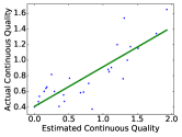
(b) continuous

Figure 4: Estimated and Actual Worker Quality

Consistent Quality for Different Attributes. We collected statistics from the Restaurant dataset to support our assumption in truth inference: a worker has consistent quality over different datatypes of attributes. In Figure 3, we plot a heat map, with the x-axis representing the 25 workers who have given the largest number of answers and the y-axis representing categorical attributes ‘Aspect’ and ‘Sentiment’ and continuous attributes ‘StartTarget’ and ‘EndTarget’. Different colors are aligned to standard deviation values (above the colorbar) for continuous attributes and error rates (below the colorbar) for categorical attributes. The color of each pixel represents the average error of answers given by worker $u$ to the tasks on attribute $j$. For a categorical attribute $j$, the error is the percentage of wrong answers. For a continuous attribute $j$, the error is the standard deviation of the differences between the answers and the ground truth. The red color (far right) implies larger error and lower worker quality, while the blue color (far left) means smaller error and better worker quality. Observe that the workers have consistent performance for categorical and continuous attributes. In addition, the colors for the same worker are similar regardless the attribute type, which means that each worker’s actual quality is consistent among different attributes.

Calibration to the Actual Quality. Figure 4 shows that our estimated quality of a worker is close to the actual quality. Each point represents a worker and the x-axis value is the quality estimated by our method while the y-axis value is the actual worker’s quality. We also show the result of a linear regression. Observe the strong correlation between our estimated quality and actual quality; the correlation coefficient is 0.844 for categorical attributes and 0.841 for continuous attributes.

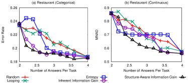
Figure 5: Effectiveness of Assignment Heuristics

6.4.2 Assignment Heuristics

We evaluate the performance of different assignment heuristics. Note that for all of them, we use our inference approach (Section 4.3). The tested heuristics are listed as follows:
$\bullet$ Random: randomly chooses the task assigned to the worker.
$\bullet$ Looping: selects the next task in a round-robin manner.
$\bullet$ Entropy: greedily chooses the next task which has the highest uncertainty (defined as entropy).
$\bullet$ Inherent Information Gain: proposed in Section 5.1.
$\bullet$ Structure-Aware Information Gain: proposed in Section 5.2.

Figure 5 presents the Error Rate and MNAD as a function of number of tasks assigned to the workers on Restaurant. The results on the other datasets are similar and omitted for the interest of space. Random and Looping select tasks without considering the answers collected so far, so they converge slowly. Entropy is biased toward selecting continuous tasks over categorical first; hence, this heuristic reduces the MNAD fast, but not the Error Rate. Inherent and Structure-Aware Information Gain consider the continuous and categorical tasks fairly and decrease the Error Rate and MNAD simultaneously. Besides, Structure-Aware Information Gain converges faster than Inherent Information Gain w.r.t. MNAD because it also considers the correlations between attributes. Recall that we use Structure-Aware Information Gain as our default method.

	correct	wrong
correct	589	90
wrong	98	35

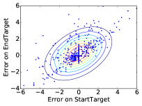
Figure 6: Correlation Among Attributes

6.4.3 Correlation Among Attributes

We perform one more experiment to support our assumption that there exist correlations among attributes, by analyzing the answers of workers.

Figure 6 shows the experimental results. In the left part of the figure observe that attributes ‘Aspect’ and ‘Sentiment’ have strong correlation. Specifically, if a worker answers ‘Aspect’ correctly, the probability to answer ‘Sentiment’ correctly is 86%. However, if a worker answers ‘Aspect’ wrongly, the probability to answer ‘Sentiment’ correctly is only 73%. In the right part of the figure, we plot a scatter diagram, with each point representing a worker’s error on attributes ‘StartTarget’ and ‘EndTarget’. We use maximum likelihood estimation to obtain the joint distribution of errors on these two attributes as described in Section 5.2. We observe a positive correlation between errors on attributes ‘StartTarget’ and ‘EndTarget’, which justifies our proposed Structure-Aware Information Gain method that considers correlations among attributes. For example, if the error of ‘StartTarget’ is 0, the distribution of ‘EndTarget’ error is $\mathcal{N}(0.28,0.76)$. However, if the error of ‘StartTarget’ is 6, the distribution of ‘EndTarget’ error is $\mathcal{N}(3.75,0.76)$. In other words, knowing the exact answer of a worker on one attribute can help to predict his answer distribution for other attributes better.

6.5 Synthetic Data

In this section, we use two types of synthetic data, in order to test the performance of our truth inference approach in cases not covered by the real data settings.

6.5.1 Tests on tables with different properties

We assess the performance of T-Crowd in terms of truth inference effectiveness by changing the following parameters of our data generator: the number of columns $M$, the ratio of categorical to the total number columns $R$ and the average difficulty of tasks $\mu\{\alpha_{i}\beta_{j}\}$. The default parameters are $M=10$, $R=0.5$ and $\mu\{\alpha_{i}\beta_{j}\}=1$. The rest of the settings are as follows:

Worker Sequence and Worker Quality: We use the same number of workers as that in our real experiments for the dataset Celebrity and assume that the workers arrive in the same sequence and that they have the same quality as in the real experiment.

Data and Ground Truth Generation: We implemented a generator for a table that takes as input the number of rows $N$ and columns $M$, and the datatype and domain range of each column. The number of possible answers in a categorical column is generated from a uniform distribution $U(2,10)$. The domain of a continuous column is $[0,1000]$. The ground truth $T_{ij}$ of each cell $c_{ij}$ is generated by selecting a value in the corresponding domain randomly.

Workers’ Answers: For each worker in sequence, his answer at each cell needs to be generated. The answer $a_{ij}^{u}$ of each worker $u$ at each cell $c_{ij}$ is created based on the ground truth $T_{ij}$ and his quality $q_{u}$, based on Eq. 1 and 3.

For fairness to all methods and since we focus on truth inference, we simulate the assignment strategy used in AMT, i.e., each task gets the same number of answers. For different parameters, we generate new datasets one hundred times and average the results to obtain the error rate and MNAD. We also run other inference methods and found that our method is dominant both on error rate and MNAD.

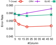
(a) Categorical Columns

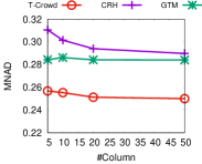
(b) Continuous Columns

Figure 7: Effect of the Number of Columns

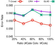
(a) Categorical Columns

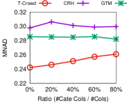
(b) Continuous Columns

Figure 8: Effect of Ratio of Columns

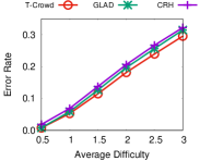
(a) Categorical Columns

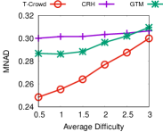
(b) Continuous Columns

Figure 9: Effect of Average Difficulty

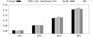
(a) Error Rate

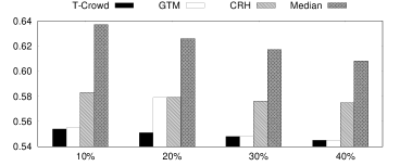
(b) MNAD

Figure 10: Noisy Datasets

Figure 11: Efficiency of Assignment

Results. In the first experiment, we vary the number of columns from 5 to 50. Figure 7 shows that the error rate and MNAD decline gradually when the number of columns increases, showing that T-Crowd infers the quality of each worker and estimates truth more accurate if we have more data. Besides our method is significantly better than the other two approaches. Next, we vary the ratio of categorical attributes from 0% to 100%. Figures 8(a) and Figure 8(b) show that our method’s error rate and MNAD do not change much when the ratio varies. Finally, we vary the average difficulty of each cell $c_{ij}$ (i.e., the average $\alpha_{i}\beta_{j}$, as defined in Section 4.2) from 0.5 to 3. High difficulty implies that the probability that workers answer correctly decreases, hence the error rate and MNAD increase as shown in Figure 9. For easier tasks, our method is significantly better than the others, but when the average difficulty is high, which means that the workers’ answers are not credible, all methods perform badly.

6.5.2 Noise in Workers’ Answers

To further demonstrate the advantage of our proposed approach T-Crowd, we conduct simulation experiments by adding noise to the original data collected for Celebrity dataset. We vary the percentage $\gamma$ of altered original answers by the workers from 10% to 40% (i.e., $\gamma$ is the percentage of answers with added noise).

For a categorical answer, we randomly select a new label from its domain and replace the original label. For a continuous answer, Gaussian noise is added. We first preprocess this answer by transforming it into its z-score. A new normalized answer is generated by adding the noise which was generated by a Gaussian distribution $\mathcal{N}(0,1)$. We finally change it to the original scale and obtain the new answer. We randomly choose $NM\gamma$ answers with replacement to add noise and the rest of the answers stay the same.

For different levels of noise $\gamma$, we generate new datasets one hundred times. For each method, we run experiments three times to smoothen out possible instabilities. Hence we run in total 300 simulations for each method and average them to obtain the error rate and MNAD for different levels of noise $\gamma$.

Figure 10(a) and 10(b) show the results. The error rate increases while MNAD declines when $\gamma$ increases. The reason for the decrease of MNAD is that the normalization denominator is the standard deviation of answers in each column. The growth rate of standard deviation is higher than that of RMSE which makes MNAD to decline.

T-Crowd performs well and stably when the level of noise $\gamma$ increases both in terms of error rate and MNAD. T-Crowd has a very similar error rate and MNAD to CRH and GTM, respectively.

6.6 Efficiency

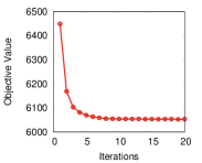
(a) Convergence Rate

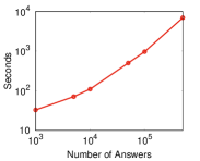
(b) Running Time

Figure 12: Efficiency of Truth Inference

In this section, we evaluate the efficiency of T-Crowd. We first investigate the truth inference cost on Celebrity dataset and then show its running time on a single machine. Figure 12(a) shows the change of the objective value in truth inference at each iteration. Note that our inference model converges to the estimated value, after only a few iterations.

We confirm the low cost of truth inference by measuring the throughput of T-Crowd, i.e., how many answers it can process per second. For this purpose, we use the synthetic data used in Section 6.5, as the number of answers collected for real data are limited. Figure 12(b) shows that the runtime of T-Crowd is approximately linear to the number of answers; T-Crowd can process approximately 100 answers per second on a single machine. This performance is acceptable, given that the rate of incoming answers is much lower in a real crowdsourcing system. It corresponds to the time complexity $\mathcal{O}(wvl\cdot|\mathcal{A}|)$ at the end of Section 4.3.

Finally, we measure the time required to assign a new task to an incoming worker on the Celebrity dataset. We assume that we already obtain the estimated truth from truth inference method. We show the running time of computing the structure-aware information gain for all candidate tasks each time a new worker arrives. Because it is easy to parallelize task assignments, we run eight processes on our machine. As shown in Figure 11, the assignment cost increases linearly with the average number of answers collected so far for each task. This is consistent to our complexity analysis at the end of Section 5.1, which suggests that the cost is linear to the total number $|\mathcal{A}|$ of answers so far. Still, as the figure shows, new assignments can be conducted in real-time, which is important for a real crowdsourcing platform.

7 conclusions

In this paper we design a unified crowdsourcing framework for collecting multi-type tabular data. Most existing methods, which are designed for simple tasks that are all of the same datatype are not effective enough in terms of both truth inference and task assignment. Based on the characteristics of tabular data, we propose a probabilistic truth inference model that unifies worker quality on both categorical and continuous datatypes. Besides, we improve the accuracy of truth inference by considering the variance in the difficulty of different tasks. In addition, we design an information gain function which we use for selecting the tasks to assign to workers, based on the current answers and the workers’ quality. We extend this function to consider the correlation in the quality of certain worker’s answers for the same entity. Our experiments on three real datasets and synthetic datasets confirm the superiority of our methods, both in truth inference and task assignment compared to the state-of-the-art.

In the future, we plan to conduct experiments with larger tables compared to the ones we have used in Section 6. In addition, we plan to extend our approach to apply on tables for which entities are not known. In this case, entities should also be collected from the crowd. A third direction is the acceleration of truth inference and task assignment by parallel and/or distributed computation as discussed at the end of Section 5.1. Finally, we will explore the possible improvement of our approach by exploiting the possible correlations between entities (not only attributes), e.g., a worker may be more familiar to celebrities starring in a certain category of films or shows.

References

- [1] Amazon Mechanical Turk. https://www.mturk.com/mturk/.
- [2] AMT External Question. http://docs.aws.amazon.com/AWSMechTurk/latest/AWSMturkAPI/ApiReference_ExternalQuestionArticle.html.
- [3] Entropy. https://en.wikipedia.org/wiki/Entropy_(information_theory).
- [4] ERF Function. http://mathworld.wolfram.com/Erf.html.
- [5] R. Boim, O. Greenshpan, T. Milo, S. Novgorodov, N. Polyzotis, and W.-C. Tan. Asking the right questions in crowd data sourcing. In ICDE, pages 1261–1264. IEEE, 2012.
- [6] B.-C. Chen, C.-S. Chen, and W. H. Hsu. Cross-age reference coding for age-invariant face recognition and retrieval. In ECCV, pages 768–783, 2014.
- [7] X. Chen, Q. Lin, and D. Zhou. Optimistic knowledge gradient policy for optimal budget allocation in crowdsourcing. In ICML, pages 64–72, 2013.
- [8] S. Das, P. S. GC, A. Doan, J. F. Naughton, G. Krishnan, R. Deep, E. Arcaute, V. Raghavendra, and Y. Park. Falcon: Scaling up hands-off crowdsourced entity matching to build cloud services. In Proceedings of the 2017 ACM International Conference on Management of Data, pages 1431–1446. ACM, 2017.
- [9] A. P. Dawid and A. M. Skene. Maximum likelihood estimation of observer error-rates using the em algorithm. Applied statistics, pages 20–28, 1979.
- [10] G. Demartini, D. E. Difallah, and P. Cudré-Mauroux. Zencrowd: leveraging probabilistic reasoning and crowdsourcing techniques for large-scale entity linking. In WWW, pages 469–478, 2012.
- [11] A. P. Dempster, N. M. Laird, and D. B. Rubin. Maximum likelihood from incomplete data via the em algorithm. Journal of the royal statistical society. Series B (methodological), pages 1–38, 1977.
- [12] X. L. Dong, L. Berti-Equille, and D. Srivastava. Integrating conflicting data: the role of source dependence. PVLDB, 2(1):550–561, 2009.
- [13] J. Fan, G. Li, B. C. Ooi, K.-l. Tan, and J. Feng. icrowd: An adaptive crowdsourcing framework. In SIGMOD, pages 1015–1030. ACM, 2015.
- [14] M. J. Franklin, D. Kossmann, T. Kraska, S. Ramesh, and R. Xin. Crowddb: answering queries with crowdsourcing. In SIGMOD, pages 61–72. ACM, 2011.
- [15] P. G. Ipeirotis, F. Provost, and J. Wang. Quality management on amazon mechanical turk. In SIGKDD workshop on human computation, pages 64–67, 2010.
- [16] A. R. Khan and H. Garcia-Molina. Crowddqs: Dynamic question selection in crowdsourcing systems. In Proceedings of the 2017 ACM International Conference on Management of Data, pages 1447–1462. ACM, 2017.
- [17] Q. Li, Y. Li, J. Gao, L. Su, B. Zhao, M. Demirbas, W. Fan, and J. Han. A confidence-aware approach for truth discovery on long-tail data. PVLDB, 8(4):425–436, 2014.
- [18] Q. Li, Y. Li, J. Gao, B. Zhao, W. Fan, and J. Han. Resolving conflicts in heterogeneous data by truth discovery and source reliability estimation. In SIGMOD, pages 1187–1198. ACM, 2014.
- [19] Y. Li, Q. Li, J. Gao, L. Su, B. Zhao, W. Fan, and J. Han. Conflicts to harmony: A framework for resolving conflicts in heterogeneous data by truth discovery. TKDE, 28(8):1986–1999, 2016.
- [20] X. Liu, M. Lu, B. C. Ooi, Y. Shen, S. Wu, and M. Zhang. Cdas: a crowdsourcing data analytics system. PVLDB, 5(10):1040–1051, 2012.
- [21] F. Ma, Y. Li, Q. Li, M. Qiu, J. Gao, S. Zhi, L. Su, B. Zhao, H. Ji, and J. Han. Faitcrowd: Fine grained truth discovery for crowdsourced data aggregation. In SIGKDD, pages 745–754. ACM, 2015.
- [22] A. Marcus, E. Wu, D. R. Karger, S. Madden, and R. C. Miller. Crowdsourced databases: Query processing with people. Cidr, 2011.
- [23] P. Mavridis, D. Gross-Amblard, and Z. Miklós. Using hierarchical skills for optimized task assignment in knowledge-intensive crowdsourcing. In WWW, pages 843–853, 2016.
- [24] J. V. Michalowicz, J. M. Nichols, and F. Bucholtz. Handbook of differential entropy. CRC Press, 2013.
- [25] H. Park, H. Garcia-Molina, R. Pang, N. Polyzotis, A. Parameswaran, and J. Widom. Deco: A system for declarative crowdsourcing. PVLDB, 5(12):1990–1993, 2012.
- [26] H. Park and J. Widom. Crowdfill: Collecting structured data from the crowd. In SIGMOD, pages 577–588. ACM, 2014.
- [27] M. Pontiki, D. Galanis, J. Pavlopoulos, H. Papageorgiou, I. Androutsopoulos, and S. Manandhar. Semeval-2014 task 4: Aspect based sentiment analysis. In SemEval, pages 27–35, 2014.
- [28] H. Rahman, S. B. Roy, S. Thirumuruganathan, S. Amer-Yahia, and G. Das. Task assignment optimization in collaborative crowdsourcing. In ICDM, pages 949–954. IEEE, 2015.
- [29] S. B. Roy, I. Lykourentzou, S. Thirumuruganathan, S. Amer-Yahia, and G. Das. Task assignment optimization in knowledge-intensive crowdsourcing. VLDBJ, 24(4):467–491, 2015.
- [30] R. Snow, B. O’Connor, D. Jurafsky, and A. Y. Ng. Cheap and fast—but is it good?: evaluating non-expert annotations for natural language tasks. In EMNLP, pages 254–263. Association for Computational Linguistics, 2008.
- [31] V. Verroios, H. Garcia-Molina, and Y. Papakonstantinou. Waldo: An adaptive human interface for crowd entity resolution. In Proceedings of the 2017 ACM International Conference on Management of Data, pages 1133–1148. ACM, 2017.
- [32] J. Wang, T. Kraska, M. J. Franklin, and J. Feng. Crowder: Crowdsourcing entity resolution. Proceedings of the VLDB Endowment, 5(11):1483–1494, 2012.
- [33] J. Whitehill, T.-f. Wu, J. Bergsma, J. R. Movellan, and P. L. Ruvolo. Whose vote should count more: Optimal integration of labels from labelers of unknown expertise. In NIPS, pages 2035–2043, 2009.
- [34] X. Yin, J. Han, and S. Y. Philip. Truth discovery with multiple conflicting information providers on the web. IEEE Transactions on Knowledge and Data Engineering, 20(6):796–808, 2008.
- [35] X. Yin, J. Han, and S. Y. Philip. Truth discovery with multiple conflicting information providers on the web. TKDE, 20(6):796–808, 2008.
- [36] H. Zhang, Y. Ma, and M. Sugiyama. Bandit-based task assignment for heterogeneous crowdsourcing. Neural computation, 2015.
- [37] B. Zhao and J. Han. A probabilistic model for estimating real-valued truth from conflicting sources. Proc. of QDB, 2012.
- [38] Y. Zheng, G. Li, and R. Cheng. Docs: a domain-aware crowdsourcing system using knowledge bases. PVLDB, 10(4):361–372, 2016.
- [39] Y. Zheng, J. Wang, G. Li, R. Cheng, and J. Feng. Qasca: a quality-aware task assignment system for crowdsourcing applications. In SIGMOD, pages 1031–1046. ACM, 2015.
- [40] D. Zhou, S. Basu, Y. Mao, and J. C. Platt. Learning from the wisdom of crowds by minimax entropy. In Advances in Neural Information Processing Systems, pages 2195–2203, 2012.
- [41] H. Zhuang, A. Parameswaran, D. Roth, and J. Han. Debiasing crowdsourced batches. In SIGKDD, pages 1593–1602. ACM, 2015.