The discrete moment problem with nonconvex shape constraints
Abstract
The discrete moment problem is a foundational problem in distribution-free robust optimization, where the goal is to find a worst-case distribution that satisfies a given set of moments. This paper studies the discrete moment problems with additional “shape constraints” that guarantee the worst case distribution is either log-concave or has an increasing failure rate. These classes of shape constraints have not previously been studied in the literature, in part due to their inherent nonconvexities. Nonetheless, these classes of distributions are useful in practice. We characterize the structure of optimal extreme point distributions by developing new results in reverse convex optimization, a lesser-known tool previously employed in designing global optimization algorithms. We are able to show, for example, that an optimal extreme point solution to a moment problem with moments and log-concave shape constraints is piecewise geometric with at most pieces. Moreover, this structure allows us to design an exact algorithm for computing optimal solutions in a low-dimensional space of parameters. Moreover, We describe a computational approach to solving these low-dimensional problems, including numerical results for a representative set of instances.
Keywords: Robust optimization, moment problem, log-concave, increasing failure rate, nonconvex optimization, reverse convex programming
1 Introduction
The moment problem is a classical problem in analysis and optimization, with roots dating back to the middle of the nineteenth century. At that time, the goal there was to seek to bound tail probabilities and expectations with given distributional moment information. Pursuing this initial goal remains active to the present day. For example, Bertsimas and Popescu [8] provides tight closed form bounds of with given first three moments of a random variable . He et al. [24] extends the problem for random variables given first, second and forth order moments, which also provided the first nontrivial bound for .
Beyond these foundational questions, the moment problem serves as an important building block in a variety of applications in the stochastic and robust optimization literatures [44, 42, 48, 47, 51]. In particular, moment problem are foundational to distribution-free robust optimization, where insight into the structure of optimal measures can be used to devise algorithms and describe properties of optimal decisions. A classic example of this approach is due to Scarf et al. [49] who leverages the fact that an optimal solution to the moment problem given the first two moments is a sum of two Dirac measures. This insight provides an analytical formula for the optimal inventory decision in a robust version of the newsvendor problem. There is a vast literature on robust optimization that builds on these initial insights in a variety of facets (see, for instance, [20, 16, 27, 4, 11, 36, 18, 14, 28] among many others).
The focus of this paper is the discrete moment problem, an important special case of the general moment that is less well-studied in the literature. In the discrete moment problem, the underlying sample space is a discrete set. The work of Prékopa (see for instance Prékopa [43]) made a fundamental contribution by devising efficient linear programming methods to study discrete moment problems. These approaches remain state-of-the-art and has seen application in numerous areas including project management [46] and network reliability [45]. Project management has also been studied in the robust optimization (see, for instance, [10]).
In classical versions of the moment problem (including the works by Prékopa and his co-authors just cited), the only constraints arise from specifying a finite number of moments. One criticism of this approach is that it can result in bounds and conclusions that may be too weak to be meaningful, or in the case of robust optimization with only moment constraints, result in decisions that are too conservative. For instance, Scarf’s solution for the newsvendor problem may even suggest to not order any inventory even when the profit margin is high [41]. This has driven researchers to introduce additional constraints, including those on the shape of the distribution. For example, Perakis and Roels [41] study the newsvendor problem leveraging non-moment information, including symmetry and unimodality. Han et al. [21] study the newvendor problem relaxing the usual assumption of risk neutrality. Saghafian and Tomlin [48] analyze the problem with the bound of tail probability and Karthik et al. [28] recently developed closed-form solutions under asymmetric demand information. In all cases, more intuitive and less conservative inventory decisions result, when compared to the classical setting with moment information alone. Other robust optimization papers that consider shape constraints include Li et al. [35] who study the chance constraints and conditional Value-at-Risk constraints when the distributional information consists of the first two moments and unimodality, Lam and Mottet [31] who study tail distributions with convex-shape constraints, and Hanasusanto et al. [23] who study the multi-item newsvendor problems with multimodal demand distributions.
However, introducing shape constraints brings new theoretical challenges. A seminal paper by Popescu [42] provides a general framework for studying continuous moment problems under shape constraints that includes, among others, symmetry and unimodality. These moment problems are formulated as semi-definite programs (SDPs) that are polynomial time solvable. Perakis and Roels [41] also employ Popescu’s framework to provide analytical robust solutions to the newsvendor problem under shape constraints that are better behaved than classical Scarf solutions. For the discrete moment problem, we are aware of only one paper [50] that considers shape constraints. Subasi et al. [50] adapt Prékopa’s linear programming (LP) methodology to include unimodality, which is modeled by an additional set of linear constraints.
Both Popescu [42] and Subasi et al. [50] illustrate how a certain class of constraints can be adapted into existing computational frameworks, SDP-based in the case of Popescu and LP-based in the case of Subasi et al.. However, there remains relevant shape constraints that are practical significant and do not naturally fit into these settings. In this paper we focus on two shape constraints: log-concavity (LC) and the increasing failure rate (IFR) property of discrete distributions (these are defined in Section 2 below). Here, we briefly highlight the importance and the applications for each class of distributions.
-
(i)
LC measures arise naturally in many applications. For example, Subasi et al. [50] illustrate how the length of a critical path in a PERT model where individual task times are described by beta distributions has a LC distribution but its other properties (other than moments inferred by the beta distributions) are unknown. Log-concavity has a wide range of applications to statistical modeling and estimation [52], e.g., Duembge et al. [17] show how the log-concavity allows the estimation of a distribution based on arbitrarily censored data (which is a common form of data for demand observations). The log-concavity also plays a critical role in economics [3]. For example, in contract theory, one commonly assumes that an agent’s type is a LC random variable [30]. The log-concavity of a distribution function has also been widely used in theory of regulation [6, 34], and in characterizing efficient auctions [39, 37].
-
(ii)
IFR distributions also play an important role in numerous applications in fields as wide-reaching as reliability theory [5], inventory management [19], revenue management [32] and contract theory [15, 33]. One reason for the prevalence IFR distributions in applications is that IFR distributions are closed under sums of random variables (and the associated convolutions of distribution functions). This is not the case for the shape properties studied by others, including symmetry and unimodality. The IFR property is useful in applications for simplifying optimality conditions to facilitate the derivation of properties of optimal decisions that yield managerial insights.
In Section 2 we show that the standard characterizations of discrete LC and IFR distributions, when added to the moment problem, make the resulting problem nonconvex and thus not amenable to either an SDP or LP formulation. Indeed, when Subasi et al. [50] derive LC distributions in their applications, they relax the LC property to unimodality, a shape constraint that can be approached by LP techniques.
At this point, one could turn to approximation methods, including conic-optimization techniques to solve the resulting nonconvex formulation. It is well known that the copositive cone and its dual are powerful tools to could convert nonconvex problems equivalently into convex ones (see, e.g., [40, 53, 12, 22]). For instance, the LC discrete moments problem considered here can be cast as a completely positive conic problem [40]. Despite this convexity, the resulting problem is still computationally intractable and further relaxation is required to obtain an approximate solution.
We do not follow an approximation approach. The nonconvexities that arise in our problems are of a certain type that can be leveraged to provide an exact global optimization algorithm and analytical results on the structure of optimal solutions. Indeed, the feasible regions have reverse convex properties (as introduced in [38] and later developed in [25] among others). A set is reverse convex if its complement is convex. Reverse convex programming is a little-studied field that has largely found application in the global optimization literature (see, for instance, Horst and Thoai [26]). To our knowledge, this theory has not been applied in the robust optimization literature.
In Section 3 we extend standard results in the reverse convex programming literature (in particular, those of [25]) so that they are applicable to our setting by introducing the notion of reverse convexity relative to another set. The main benefit is that we can show reverse convex programs of this type have the following appealing structure — there exist optimal extreme point solutions with a basic feasible structure analogous to basic feasible solutions in linear programming. The basic feasible structure reveals (in Section 4) that optimal extreme point distributions in the LC and IFR settings have piecewise geometric structure. This analytical characterization allows for solving these moment problems as low-dimensional systems of polynomials equations. We propose a specialized computation scheme for working with such systems. This allows us to provide numerical bounds on probabilities that are tighter than those in the existing literature, including those bounds that leverage unimodal shape constraints (see Section 5). All proofs not in the main text are included in the appendix.
Summary of contributions
The main focus of the paper is on theoretical properties of LC and IFR-constrained moment problems, where we provide structural results on optimal solutions. For the LC case we show there exists optimal solutions that are piecewise geometric, and for the IFR case we show the tail probabilities of optimal distributions are piecewise geometric.
Our structural results and computational approaches suggest a wide range of applications due the prevalence of these classes of shape-constraints in real applications, as discussed above. Our results can provide new bounds on tail inequalities (i.e., ) for a random variable under moment and shape constraints. We provide a numerical framework for computing these bounds.
Moreover, the techniques developed in this paper allow us to solve an inner maximization problem with LC and IFR constraints. Our structural results could prove useful in solving the outer minimization problem in a robust optimization framework. Indeed, solution approaches to the standard max-min robust optimization formulation benefit greatly when the inner maximization problem has analytical structure.
Finally, we prove a new result on a generalized form of reverse convex optimization (Theorem 3.6) that may be of independent interest, with potential applications to other nonconvex optimization problems.
Notations
We use the following notation throughout the paper. Let denote the set of real numbers and the vector space of -dimensional real vectors. Moreover, let denote the set of -dimensional vectors with all nonnegative components and denote the set of -dimensional vectors will all positive components. The closure of the set in (in the usual topology) is denoted and its boundary by . Let denote the expectation operator and the indicator function of set .
Let denote the set of consecutive integers, starting with integer and ending with integer . Similarly, let . We will not have occasion to use and in their usual sense as intervals in , so there is no chance for confusion. For , positive integers, denotes the binomial coefficient of choose ; that is, it counts the number of ways to choose -subsets of objects.
2 The discrete moment problem with nonconvex shape constraints
We study the classical problem of moments with moments (cf. [42]):
| s.t. |
where is a subset of measures on the measurable space (with elements denoted by ) with -algebra , is a measurable function and for . We take to ensure that is a probability measure and the remaining constraints correspond to requiring the measure has as its first moments.
Our focus is where is a finite set of real numbers and is the power set of . In fact, we assume that and so (however, see Section 5.1 where we have occasion to rescale the ). In this setting, a measure can be represented by a nonnegative -dimensional vector where and for . We will refer to the vector as a distribution and often suppress the measure that it represents. This yields the following discrete moment problem (DMP):
| (1a) | |||||
| s.t. | (1b) | ||||
| (1c) | |||||
We study (1) for two specifications of the set of distributions in constraint (1c).
Definition 2.1 (cf. Definition 2.2 in [13]).
A distribution is discrete log-concave (or simply log-concave or (LC)) if (i) for any such that then ; and (ii) for all , . We let denote the class of all LC distributions.
More precisely, (i) implies that for every LC distribution there exists a consecutive support for some such that for and otherwise. For an LC distribution with support we must then ensure holds for . At all other the inequality is trivial because at least one of or is zero.
Definition 2.2 (cf. Definition 2.4 in [13]).
A distribution has an increasing failure rate (IFR) if the failure rate sequence is a non-decreasing sequence; that is, for all . We let denote the class of all IFR distributions.
It is well-known that is a strict subset of [2]. It is relatively straightforward to see that the sets and are nonconvex. However, they share one additional common feature that is critical to our approach.
Definition 2.3.
A set in is reverse convex if for some convex set . A set is said to be reverse convex with respect to (w.r.t) a set if for some convex set .
In the remainder of this section we show that the problem (DMP) when setting be or all have constraints that are reverse convex w.r.t. . This common fact is leveraged to solve these related problems to global optimality in a unified framework.
The seemingly more or less straightforward generalization to reverse convexity w.r.t. , however, could lead to a significantly different analytical properties. For example, observe that if a function is quasiconcave (over ) then its lower level sets are reverse convex. However, a function whose lower level sets are reverse convex w.r.t. some strict subset of need not be quasiconcave. In Section 3 we show that problems with reverse convex structure can be approached using a novel optimization technique that extends the pioneering work of [25].
2.1 The moment problem over log-concave distributions
Consider problem (DMP) when . We separate the optimization over into first determining a support (mapping to condition (i) of Definition 2.1) and then introducing inequalities of the form for in that support (mapping to condition (ii) in Definition 2.1). This yields the two-stage optimization problem:
| (2a) | |||||
| s.t. | (2b) | ||||
| (2c) | |||||
| (2d) | |||||
| (2e) | |||||
The strict constraints (2d) make the feasible region appear not to be closed. However, the following reformulation of (DMP-LC) reveals that the feasible region can be described with non-strict inequalities and is thus closed:
| (3a) | |||||
| s.t. | (3b) | ||||
| (3c) | |||||
| (3d) | |||||
In (DMP-LC’) there is no outer maximization over the support between and .
Proposition 2.4.
Problems (DMP-LC) and (DMP-LC’) are equivalent.
Proposition 2.5 below shows that (DMP-LC’) is a nonconvex optimization problem where constraint (3c) defines a reverse convex set w.r.t. .
Proposition 2.5.
The set is convex for any positive integers and .
Whereas the set is convex, the set where nonnegativity is relaxed – that is, – is not convex. Indeed, and are in but is not in . This means that is not quasiconcave on its domain.
2.2 The moment problem over increasing failure rate distributions
Consider problem (DMP) with . The following result illustrates a tight connection between the IFR case and the LC case. This result is known in the continuous case (see [5, Chapter 2]), we provide details for the discrete analogue that is the focus of this paper.
Lemma 2.6.
A distribution has an increasing failure rate if and only if its tail probability sequence is log-concave, where .
In the IFR case, (DMP) becomes
| (4a) | |||||
| s.t. | (4b) | ||||
| (4c) | |||||
Using the transformation described in Lemma 2.6, where denotes tail probabilities, we can reformulate (4) as
| (5a) | |||||
| s.t. | (5b) | ||||
| (5c) | |||||
| (5d) | |||||
| (5e) | |||||
where are set to . Constraint (5c) captures the log-concavity of the tail probabilities and (5d) captures the non-increasing property of tail probabilities. There is no need to consider an outer optimization over supports and use strict inequalities to capture the property of consecutive supports. The consecutiveness of supports is immediate from the monotonicity condition of the . Indeed, once for some then for all by monotonicity.
3 A special class of nonconvex optimization problems
In this section we present a general class of problems that includes all the problems introduced in Section 2 as special cases. This class admits optimal extreme point solutions that are determined by setting a sufficient number of inequalities to equalities. This result is reminiscent of linear programming where extreme points have algebraic characterizations as basic feasible solutions.
Our analysis proceeds in two stages. First, we discuss a broad class of optimization problems that have optimal extreme point solutions. Second, we specialize this general class to a class of nonconvex optimization problems where the source of nonconvexity arises from reverse convex sets (see Definition 2.3). This work extends some of theory on reverse convex optimization, initiated by [25] but tailors these results to the discrete moment problem. To our knowledge, these results are not subsumed by others in the existing literature.
3.1 Linear optimization over (nonconvex) compact sets
Let us first consider a very general optimization problem:
| (6) | ||||
where is a lower semicontinuous and quasiconcave function and is nonempty and compact (closed and bounded) subset of . It is worthwhile to note that the results in this section can be generalized to any locally convex topological vector space in the sense of Aliprantis and Border [1, Chapter 5]. This is not required for the study of the discrete moment problem, but is potentially relevant for an exploration of the continuous case that follows a similar line of inquiry.
The goal of this subsection is to prove the following:
Theorem 3.1.
There exists an optimal solution to (6) that is an extreme point of .
Recall that an extreme point of is any point where the set of such that for some is empty. Let denote the extreme points of the set . The special case to Theorem 3.1 where is convex well-known and immediate from Aliprantis and Border [1, Corollary 7.75]:
Lemma 3.2.
If is compact and convex then (6) has an optimal extreme point solution.
The proof when is not convex takes a couple more steps. The first step is to work with the closed convex hull of , which is the intersection of all closed convex sets that contain .
Lemma 3.3.
(Theorem 5.3 in [1]) The closed convex hull of a compact set is compact. In particular, is a compact convex set.
The following lemma helps us to leverage these results about closed convex hulls to learn about the original problem (6).
Lemma 3.4.
Let be a compact subset of . Then .
We prove Theorem 3.1 using Lemmas 3.3 and 3.4 in Section A.4 of the online supplement.
3.2 Reverse convex optimization problem with nonnegative constraints
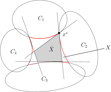
The following lemma captures the essence of reverse convex optimization and serves as motivation and a visualization tool for understanding our main theoretical result below (see Theorem 3.6).
Lemma 3.5.
Consider the optimization problem
where is a lower semicontinuous and quasiconcave function, , and the are closed, reverse convex sets such that is a nonempty and compact subset of . Then there exists an optimal solution that lies on the boundary of at least of the sets .
Lemma 3.5 extracts some ideas from existing results (particularly from [25, Theorem 2]) and presents them in a clean, geometric form. To facilitate the understanding of this lemma, we further provide an intuitive graphical illustration in Figure 1.
Despite its elegance, this lemma is insufficient for our purposes. First, it only applies when the are reverse convex. The argument breaks down if the are reverse convex w.r.t. another convex set , as needed for the problems in Section 2. In particular, when the convex set is a polytope, even though we can use as a reverse convex set to replace , it contains the boundaries from the original polytope which are undesirable for analyzing the extreme optimum solutions. Second, the conclusion only provides a lower bound on the number of boundaries an optimal solution lies on. Although sufficient for the LC case, a strengthening that leverages the concept of linear independence — familiar from the analogous linear programming result [9, Theorem 2.3] — is needed for the IFR case.
As to the second insufficiency, a standard setting in reverse convex optimization is to consider a feasible region
and assume properties on the functions . These properties typically include differentiability assumptions (so that gradients are defined) and some form of concavity (the weakest being quasiconcavity). Under these concavity assumptions, the lower-level sets of are reverse convex and Lemma 3.5 applies so that extreme points are determined by a minimum number of tight constraints of the form . Unfortunately, those results do not apply in our setting. Indeed, the discrete moment problems we consider here does not involve quasiconcave functions, instead functions whose lower level sets are reverse convex w.r.t. the nonnegative orthant.
These considerations motivate us to establish a more general theory of reverse convex optimization. In particular, we analyze the following problem
| s.t. | ||||
| (Rev-Cvx) | ||||
where and the are functions from to and is an by , and for , the set is reverse convex w.r.t. the nonnegative orthant .
Assumption 1.
We make the following additional technical assumptions on (3.2):
-
(i)
The objective function is continuous and quasiconcave,
-
(ii)
The matrix is full-row rank,
-
(iii)
For each , is differentiable, and
-
(iv)
The feasible region is nonempty and compact.
We also need the following notation to state the main theorem of this section. For any feasible solution to (2.3) let denote the support of ; that is, . Let denote the -th row of the matrix and the -th column. For any subset of (for instance, the support of a feasible solution), let . That is, is the submatrix of consisting the columns indexed by . Recall that denotes the -th row of the matrix and let denote the span of the rows of . Finally, let denote the gradient of at , where is the gradient of restricted to the components in the subset .
Theorem 3.6.
Consider an instance of (3.2) where Assumption 1 hold. Then there exists an optimal extreme point solution.
Moreover, for any extreme point optimal solution , of the following inequalities
are tight.
In addition, letting , if we further assume that for all the tight constraints with one has , then there are of the vectors are linearly independent, where is the unit vector with in the th component and otherwise.
Theorem 3.6 is the main theoretical result in this paper. The proof largely follows the geometric intuition captured in Figure 1. At its core, it involves defining separating hyperplanes and inscribing a polyhedral set inside the feasible region. Then, the equivalence of extreme points and basic feasible solutions for the polyhedron is leveraged to establish the result.
However, the proof has additional technical challenges. It must make sense of how inequalities that describe the orthant interact with the gradients of the constraint functions . Moreover, the affine equality constraints , that correspond to the moment conditions in (1), force us to work within the affine space defined by these constraints for much of the proof. Finally, we require a spanning condition of the gradients to ensure that the full analysis can be captured in that space.
Proof of Theorem 3.6.
Since is continuous and quasiconcave and is a compact set, then by Theorem 3.1, there exists an optimal extreme point solution. For any such optimal extreme point with support define
Then the feasible region includes . Let and denote
Our goal is as follows. For , we want to construct sets of the form
| (7) |
such that
| (8) |
is a subset of , where and will be specified later. As long as , since is an extreme point of , it is an extreme point of as well. Note that is defined by a number of linear equalities and inequalities, then there must exists of them that are tight at point , and we can further check which constraint is tight.
We now construct such a . Let and
| (9) |
A key property of is that it admits a strong separation property useful for our arguments (see Claim 1 below). To describe this property, we explore a related set in a smaller subspace. Construct matrix such that its columns span the whole null space of ; That is and . Then, we have that
| (10) |
Letting
we can define the “strong separation” property of as follows.
Claim 1.
(Strong separation) For all there exists and such that
| (11) |
Moreover, if we further assume then for all .
We relegate the proof of Claim 1 to Section A.6 in the supplement and return to constructing . According to (8) it suffices to show how to construct such that
| (12) |
since . In other words, we need to prove that implies .
| , , and obtained by strong separation | |
|---|---|
| , , are obtained weak separation | |
| and |
We will show (12) in two cases: (i) ; (ii) . We use Table 1 to track some of the notation and details.
In case (i), according to Claim 1, there exists some and such that
| (13) |
By letting and , one has . Moreover, from definition (7) of , any satisfies and
This combining with (13) yields that for any . Then according to (9), such does not belong to simply because it violates the constraint . Therefore we can conclude that for all .
In case (ii), again by Claim 1, we have , where if . Then we can take and in (7). Obviously, and for any . Similarly, we can argue that such a does not belong to due to the violation of the constraint . Then it follows that for all .
So far, we have constructed in the form of (9) as in Table 1 and based on (8). Moreover, we have shown . Since is an extreme point of and lies both in and , it is an extreme point of as well. Note that is defined by a number of linear equalities and inequalities, then there must exists of them that are tight and linear independent at point , by standard theory, e.g. [9, Theorem 2.3].
Since is an by matrix of rank , there are tight constraints from
where if . Now let’s investigate which constraint in the above could be tight. First of all, it is obvious that is tight for all and could not be tight for all . Then for the constraint such that , since , cannot be tight. Finally, recall we have proved in the previous discussion that for all such that . That is, when , it holds that and thus the corresponding constraint cannot be tight at . In summary, all tight constraints come from
| (14) |
which implies of the inequalities
in (3.2) are tight. Moreover, when for all , in (14) and these tight constraints are linearly independent. In other words, the set of vectors are linearly independent, where is the gradient of the constraint . This completes the proof of Theorem 3.6. ∎
4 Characterizing optimal extreme point solutions in the discrete moment problem
Theorems 3.6 and 3.1 are powerful tools for analyzing the moment problems we discussed in Section 2. They will allow us to characterize the structure of optimal extreme point solutions. In the following two subsections we analyze the LC and IFR distributions cases from Sections 2.1 and 2.2. There is a general pattern to our analysis, which we briefly describe here.
Each problem has two alternate formulations, with one indicated by a “prime”. In the LC case these two formulations are (DMP-LC) and (DMP-LC’). The “prime” formulation has a closed and compact feasible region which allows us to leverage Theorem 3.1 to show the existence of an optimal extreme point solution . With in hand, we apply Theorem 3.6 to a small adjustment of the “non-prime” formulation that replaces strict inequalities with non-strict inequalities based on the support of . Theorem 3.6 implies that a certain number of constraints are tight, including some number of the reverse convex constraints (for instance, (2c) in (DMP-LC)). Making these constraints tight determines the structure of the optimal extreme point solutions. In the LC case, a piecewise geometric structure is obtained.
4.1 Log-concavity
Recall the two alternate formulations (DMP-LC) and (DMP-LC’). In particular, recall that there are moment constraints in (2b) and (3b).
Theorem 4.1.
Every feasible instance of (DMP-LC) has an optimal extreme point solution. Moreover, every optimal extreme point solution has the following structure: there exist (i) integers and for with where is the support of and (ii) real parameters , for such that
| (15) |
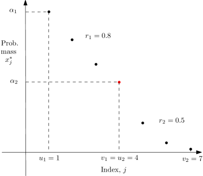
That is, there exists an optimal solution to (DMP-LC) that has a piecewise geometric structure with (at most) pieces.
Proof.
Consider the (DMP-LC’) representation of the problem. The zeroth order moment constraint ((3b) for ) is , which, along with the nonnegative constraints (3d), implies the feasible region of the problem (DMP-LC’) is compact. Then by Theorem 3.1, there exists an optimal extreme point solution to (DMP-LC’) and thus also (DMP-LC) since these problems are equivalent (via Proposition 2.4).
Let be any extreme optimal solution and for simplicity we assume its support is (the general case of suppose with follows analogously). Note that when , there are at most points in the interval , where each point , could be viewed as a single piece and the conclusion readily follows. Therefore, in the remainder of the proof we assume .
Let and define the following problem:
| (16a) | ||||
| s.t. | (16b) | |||
| (16c) | ||||
| (16d) | ||||
Note that (16) is a restriction of (DMP-LC) with a given support and replacing the strict inequalities in (2d) with non-strict inequalities in (16d). Note also that is an extreme optimal solution to (DMP-LC) and it is feasible to (16), hence is an extreme optimal solution to (16).
To uncover the structure (15) of we apply Theorem 3.6. Convert the constraint as a nonnegative constraint to mimic the nonnegativity constraint of (2.3) by making a change of variables to arrive at the following equivalent form:
| (17a) | ||||
| s.t. | (17b) | |||
| (17c) | ||||
| (17d) | ||||
Observe that is an optimal extreme point solution of (17).
We now verify that (17) satisfies the conditions of Theorem 3.6. Again, the zeroth order moment constraint guarantees the feasible region is compact. Let for . Here the index plays the role of index in Theorem 3.6. Note that (the index of the constraint functions) need not be tied to (the index of the decision variable components) in a general application of Theorem 3.6. As we have shown in Proposition 2.5, the set is convex, and it is an easy extension that and this implies that is convex. This implies that all of the conditions in Theorem 3.6 are satisfied when applied to (17).
Since the constraints cannot be tight at point for , this application of Theorem 3.6 implies that at least of the (17c) constraints are tight at , or equivalently there are at most of the (16c) constraints that are not tight at in (16c). These non-tight indexes can divide the interval into at most pieces, and within each piece we have , where , are the left and right endpoint of piece of the domain. It is a standard observation to note that such a system implies for . Setting yields the form (15). ∎
The piecewise geometric form (15) of optimal extreme point distributions to (DMP-LC) is illustrated in Figure 2.
The proof of Theorem 4.1 does not use the linear independence conditions of Theorem 3.6. A basic count of tight constraints is able to deliver the piecewise geometric structure, since the number of constraints in problem (DMP-LC) for a given support is small compared to the number of variables. Consider support in (DMP-LC). Theorem 3.6 implies that of the constraints in (2c)–(2d) are tight. Since all constraint in (2d) are strict (this is handled carefully in the proof) this implies all tight constraints are from (2c), which are of the form . Setting of these constraints to equality directly yields the geometric structure (15).
4.2 Increasing failure rate
Recall the formulation (DMP-IFR’) of the IFR moment problem in Section 2.2 with . We will show that the optimal solution has similar structure as the log-concave case, again using Theorems 3.6 and 3.1.
Here we notice two facts. First, by the log-concave constraint and the non-increasing property of , any feasible solution has a consecutive support naturally, and the support starts from . This is different from the log-concave case. Second, if there is some such that , this combined with the constraint indicates that we have . However, we also have in the problem’s constraints. This means that implies . Then by induction we have .
Combine the two facts above, the interval can be divided into three consecutive parts: , where we have , , , i.e., an all-one interval, a strictly decreasing interval, and an all-zero interval. Further, the optimal solution in the middle interval has a more detailed characterization stated here.
Theorem 4.2.
Every feasible instance of (DMP-IFR’) has an optimal extreme point solution. Moreover, for every optimal extreme point solution , there exist integers such that when , when . The interval can be divided as follows. There exist (i) integers and for with (ii) real parameters , for such that
| (18) |
We remark on an important difference in the analysis of the LC and IFR cases. Here it is not enough to have a lower bound on the number of tight constraints given by the first part of Theorem 3.6. The reason is that (DMP-IFR’) has in the order of constraints of type (using the notation of (3.2)) corresponding to constraints (5c) and (5d) in (DMP-IFR’), rather than such constraints in the LC case. This requires us to use the “in addition” part of Theorem 3.6 that invokes the linear independence of gradients. For this reason, the proof of Theorem 4.2 requires additional work.
5 An implementation with numerical results
In this section we results results in Section 4 to solve a representative sample of moment problem numerically. We focus on the moment problem over log-concave distributions with two moments as a proof of concept of our approach (these ideas carry over to the more general case). That is, we find an optimal solution to
| (19a) | ||||
| s.t. | (19b) | |||
| (19c) | ||||
| (19d) | ||||
| (19e) | ||||
using the structure of optimal extreme point solutions in Theorem 4.1. According to that theorem, there exists an optimal piecewise geometric distribution for (19) with at most pieces. Thus, we can restrict the search to finding feasible parameters , , , , , , and to construct an according to (15) that satisfies the constraints of the problem with the largest objective value. Observe that (15) captures the structure of constraints (19c)–(19e) in (DMP-LC), the choice of parameters is further restricted by the moment constraints (19b).
A more traditional approach to solving (19) would be take as the decision variable and solve (19) directly. The resulting problem is nonconvex and (potentially) high-dimensional if is large, whereas our approach remains low-dimensional as grows.
5.1 Computational approach
In this section we describe how to reduce the search for optimal extreme point solutions to (19) from a seven-dimensional decision space – , , , , , , and – to a four-dimensional decision space. The first three variables concerning the domain: and describe the support and the “break-point” between the two geometric pieces. The fourth parameter, which is denoted in the sequel, captures the geometric shape of the constraints and accounts for all of , , , and when restricted to satisfy the moment constraints (2b). We construct this parameter over the next several paragraphs.
The first step in this reduction is a normalization step. Recall that an instance of (19) is specified by the elements of the sample space and the moments and . For simplicity, we shift and scale the elements of the sample space so that the resulting distribution has mean and variance . For each subtract the mean from and scaling the result by . The resulting sample space is . That is, for . Again we make the assumption as in Section 2 that for simplicity, so that we have .
Now, we fix the support and break point . Our final algorithm will enumerate over these all possible values of , and in an outer loop. Given , , and , the remaining decision variables are , , , and . The zeroth moment condition amounts to
| (20) |
and similarly for the first and second moment conditions. In order to reduce the degrees of freedom further we manipulate the sums in (20) and introduce some additional notation. First of all, we let and observe that we can express in terms of and . Indeed, since we have at the middle point , we have , in which case we can rewrite (20) as
| (21) |
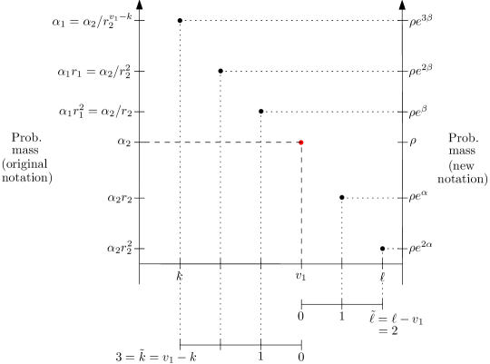
where we re-index the sums and set and . The three terms in (21) are the probability mass on the left, right, and at the middle point. Finally, for reasons that will become apparent below, we will set and for nonnegative scalars and so that (21) becomes
| (22) |
Figure 3 may assist the reader in tracking the notation in (20)–(22).
For the first and second moments, we also define the according to the indexing established in (22). Moreover, we set , in which case the moment condition amounts to
| (23) |
Similarly, the second moment condition is
| (24) |
Taken together, we have rephrased the problem to finding three unknowns – , and – in three equations (22)–(24). By first eliminating , we get two equations in two unknowns:
| (25) | ||||
| (26) |
The final step is to show that, given an , there is a unique choice of such that . Then, to identify common roots of and is equivalent to identifying the roots of a single equation , reducing the problem to a search for one unknown in one equation.
We achieve this final task by exploring monotonicity properties of . First, a direct computation yields:
where is the discrete random variable with distribution . We then use the following technical lemma.
Lemma 5.1.
Suppose the polynomial with satisfies
| (27) |
Then has at most one root when and is increasing on .
It follows from (23) that and . Now apply Lemma 5.1 to the polynomials and respectively (in the former, is and ). Supposing roots exist to these polynomials, define
such that if and only if and if and only if . If roots do not exist set and/or . Thus it suffices to focus on the region where and . As a result, when ,
Similarly for we have
In summary, we have when and when . This monotonicity yields our desired property that we can identify a mapping such that .
To apply Newton’s method to solve , must find the derivative with respect to . Observe that
and
and so
Using this derivative, Newton’s method on the interval of real numbers finds all roots of .
As a final note, when we get the solution of pairs of , we only include those that satisfy the inequality , which is translated from the log-concave constraint on the middle index .
5.2 Numerical results
To illustrate the performance of the proposed computational approach, we implement it on a concrete example that appears in the literature [50]. We note that the main focus of the paper is the theoretical properties for global optima of shape-constrained discrete moment problems instead of developing fast algorithms. Therefore, we provide this example only for illustrative purposes. A more in-depth investigation of efficient computation methods for general problems will be left as future work.
In [50], the authors aim at solving a specific discrete moment problem (Example 4) with log-concave constraint (19). However, their methodology requires relaxing the constraint to be unimodal, which they solve via a linear programming. As a type of benchmark, we compare the bounds that can be derived by our method with theirs. In detail, the specific example we solve is (19) with data specified in Table 2 below. The sample space (before scaling) is always the natural numbers up to , i.e., .
Our benchmark calculations use the unimodal relaxation of [50], described below in our notation.
| s.t. | ||||
where is the “mode” of the distribution. Instead of moment constraints, we use the binomial moment constraints of [50], i.e.
where the data can be transformed to moment data via the linear transformation: , , and . Note that this linear transformation can be extended to higher moments, see [44, Section 5.6] for details. The objective function is the probability mass on the positive values of , i.e., and provides an upper bound on the tail probability given the first two moments. Optimizing the negative of this objective also allows us to calculate lower bounds on tail probabilities. The results are shown in Table 2.
| Unimodal | Log-concave | |||||
|---|---|---|---|---|---|---|
| LB | UB | LB | UB | |||
| 5 | 1.9 | 1.3 | 0.8750 | 1 | 0.9000 | 1 |
| 5 | 2.1 | 1.3 | 0.9750 | 1 | 0.9920 | 1 |
| 5 | 1.9 | 1.7 | 0.8000 | 1 | 0.8094 | 0.8433 |
| 11 | 5.2 | 13.1 | 0.9482 | 1 | 0.9684 | 1 |
| 11 | 4.6 | 13.1 | 0.8745 | 1 | 0.8924 | 0.9026 |
| 11 | 5.2 | 15.1 | 0.9208 | 1 | 0.9310 | 0.9921 |
The LC constraint gives tighter lower and upper bounds in all cases. This is to be expected, since the unimodal relaxation is clearly a relaxation and so by solving the original log-concave version of the problem we are able to achieve tighter lower and upper bounds.
6 Conclusion
In summary, we use a reverse convex optimization approach to characterize optimal extreme point distributions for moment problems with reverse convex shape constraints. This characterization allowed us to design an exact low-dimensional algorithm for solving these problems to optimality.
There are several possible directions to apply and build on the results in this paper that we leave as future work. First, there are specific applications of robust optimization where log-concave or IFR distributions are common. One standard example is the robust newsvendor problem originally studied by [49] where having structural solutions to the second-stage moment problem can be useful in characterizing optimal inventory strategies. Second, although these results are for the discrete moment problem we believe there is scope to extend them through limiting arguments to the continuous case. Lastly, there is room to more deeply explore implementations of our computational approach that pays attention to issues of numerical stability and scaling properties.
References
- Aliprantis and Border [2006] C.D. Aliprantis and K.C. Border. Infinite Dimensional Analysis: A Hitchhiker’s Guide. Springer, third edition, 2006.
- An [1997] M.Y. An. Log-concave probability distributions: Theory and statistical testing. Duke University Dept of Economics Working Paper, 1997.
- Bagnoli and Bergstrom [2005] M. Bagnoli and T. Bergstrom. Log-concave probability and its applications. Economic Theory, 26(2):445–469, 2005.
- Bandi and Bertsimas [2012] C. Bandi and D. Bertsimas. Tractable stochastic analysis in high dimensions via robust optimization. Mathematical programming, pages 1–48, 2012.
- Barlow and Proschan [1996] R.E. Barlow and F. Proschan. Mathematical Theory of Reliability, volume 17. SIAM, 1996.
- Baron and Myerson [1982] D. P. Baron and R. B. Myerson. Regulating a monopolist with unknown costs. Econometria, 50(4), 1982.
- Ben-Tal and Nemirovski [2001] A. Ben-Tal and A. Nemirovski. Lectures on Modern Convex Optimization: Analysis, Algorithms, and Engineering Applications. SIAM, 2001.
- Bertsimas and Popescu [2005] D. Bertsimas and I. Popescu. Optimal inequalities in probability theory: A convex optimization approach. SIAM Journal on Optimization, 15(3):780–804, 2005.
- Bertsimas and Tsitsiklis [1997] D. Bertsimas and J.N. Tsitsiklis. Introduction to Linear Optimization. Athena, 1997.
- Bertsimas et al. [2006] D. Bertsimas, K. Natarajan, and C.-P. Teo. Persistence in discrete optimization under data uncertainty. Mathematical programming, 108(2):251–274, 2006.
- Bertsimas et al. [2013] D. Bertsimas, V. Gupta, and N. Kallus. Data-driven robust optimization. arXiv preprint arXiv:1401.0212, 2013.
- Burer [2009] S. Burer. On the copositive representation of binary and continuous nonconvex quadratic programs. Mathematical Programming, 120(2):479–495, 2009.
- Canonne et al. [2015] C.L. Canonne, I. Diakonikolas, T. Gouleakis, and R. Rubinfeld. Testing shape restrictions of discrete distributions. arXiv preprint arXiv:1507.03558, 2015.
- Chen et al. [2016] Z. Chen, M. Sim, and H. Xu. Distributionally robust optimization with infinitely constrained ambiguity sets. Working Paper, 2016.
- Dai and Jerath [2016] T. Dai and K. Jerath. Impact of inventory on quota-bonus contracts with rent sharing. Operations Research, 64(1):94–98, 2016.
- Delage and Ye [2010] E. Delage and Y. Ye. Distributionally robust optimization under moment uncertainty with application to data-driven problems. Operations research, 58(3):595–612, 2010.
- Duembge et al. [2011] L. Duembge, A. Huesler, and K. Rufibach. Active set and em algorithms for log-concave densities based on complete and censored data. arXiv preprint arXiv:0707.4643v4, 2011.
- Gao and Kleywegt [2016] R. Gao and A.J Kleywegt. Distributionally robust stochastic optimization with wasserstein distance. arXiv preprint arXiv:1604.02199, 2016.
- Gavirneni et al. [1999] S. Gavirneni, R. Kapuscinski, and S. Tayur. Value of information in capacitated supply chains. Management science, 45(1):16–24, 1999.
- Goh and Sim [2010] J. Goh and M. Sim. Distributionally robust optimization and its tractable approximations. Operations research, 58(4-part-1):902–917, 2010.
- Han et al. [2014] Q. Han, D. Du, and L.F. Zuluaga. Technical note: A risk and ambiguity-averse extension of the max-min newsvendor order formula. Operations Research, 62(3):535–542, 2014.
- Hanasusanto and Kuhn [2016] G.A. Hanasusanto and D. Kuhn. Conic programming reformulations of two-stage distributionally robust linear programs over wasserstein balls. arXiv preprint arXiv:1609.07505, 2016.
- Hanasusanto et al. [2015] Grani A. Hanasusanto, Daniel Kuhn, Stein W. Wallace, and Steve Zymler. Distributionally robust multi-item newsvendor problems with multimodal demand distributions. Mathematical Programming, 152(1):1–32, 2015.
- He et al. [2010] S. He, J. Zhang, and S. Zhang. Bounding probability of small deviation: A fourth moment approach. Mathematics Operations Research, 35(1):208–232, 2010.
- Hillestad and Jacobsen [1980] R.J. Hillestad and S.E. Jacobsen. Reverse convex programming. Applied Mathematics & Optimization, 6(1):63–78, 1980.
- Horst and Thoai [1999] R. Horst and N.V. Thoai. DC programming: overview. Journal of Optimization Theory and Applications, 103(1):1–43, 1999.
- Jiang et al. [2012] R. Jiang, J. Wang, and Y. Guan. Robust unit commitment with wind power and pumped storage hydro. IEEE Transactions on Power Systems, 27(2):800–810, 2012.
- Karthik et al. [2017] K. Natarajan, M. Sim, and J. Uichanco. Asymmetry and ambiguity in newsvendor models. Management Science (Articles in Advance), 2017.
- Klee [1957] V.L. Klee. Extremal structure of convex sets. Archiv der Mathematik, 8(3):234–240, 1957.
- Laffont and Tirole [1988] J.-J. Laffont and J. Tirole. The dynamics of incentive contracts. Econometria, 56(5):1153–1175, 1988.
- Lam and Mottet [2015] H. Lam and C. Mottet. Tail analysis without tail information: A worst-case perspective. arXiv preprint arXiv:1507.03293, 2015.
- Lariviere [2006] M.A. Lariviere. A note on probability distributions with increasing generalized failure rates. Operations Research, 54(3):602–604, 2006.
- Lariviere and Porteus [2001] M.A. Lariviere and E.L. Porteus. Selling to the newsvendor: An analysis of price-only contracts. Manufacturing & Service Operations Management, 3(4):293–305, 2001.
- Lewis and Sappington [1988] T.R. Lewis and D.E.M. Sappington. Regulating a monopolist with unknown demand. American Economic Review, 78(5):986–998, 1988.
- Li et al. [2016] B. Li, R. Jiang, and J.L. Mathieu. Ambiguous risk constraints with moment and unimodality information. Optimization Online. http://www.optimization-online.org/DB_HTML/2016/09/5635.html, 2016.
- Long and Qi [2014] D.Z. Long and J. Qi. Distributionally robust discrete optimization with entropic value-at-risk. Operations Research Letters, 42(8):532–538, 2014.
- Matthews [1987] S. Matthews. Comparing auctions for risk averse buyers: A buyer’s point of view. Econometrica, 55(3):633–646, 1987.
- Meyer [1970] R. Meyer. The validity of a family of optimization methods. SIAM Journal on Control, 8(1):41–54, 1970.
- Myerson and Satterthwaite [1983] R.B. Myerson and M.A. Satterthwaite. Efficient mechanisms for bilateral trading. Journal of Economic Theory, 29:265–281, 1983.
- Peña et al. [2015] J. Peña, J.C. Vera, and L.F. Zuluaga. Completely positive reformulations for polynomial optimization. Mathematical Programming, 151(2):405–431, 2015.
- Perakis and Roels [2008] G. Perakis and G. Roels. Regret in the newsvendor model with partial information. Operations Research, 56(1):188–203, 2008.
- Popescu [2005] I. Popescu. A semidefinite programming approach to optimal-moment bounds for convex classes of distributions. Mathematics of Operations Research, 30(3):632–657, 2005.
- Prékopa [1990] A. Prékopa. Sharp bounds on probabilities using linear programming. Operations Research, 38(2):227–239, 1990.
- Prékopa [2013] A. Prékopa. Stochastic Programming, volume 324. Springer Science & Business Media, 2013.
- Prékopa and Boros [1991] A. Prékopa and E. Boros. On the existence of a feasible flow in a stochastic transportation network. Operations Research, 39(1):119–129, 1991.
- Prékopa et al. [2004] A. Prékopa, J. Long, and T. Szantai. New bounds and approximations for the probability distribution of the length of the critical path. In Dynamic Stochastic Optimization, pages 293–320. Springer, 2004.
- Rujeerapaiboon et al. [2016] N. Rujeerapaiboon, D. Kuhn, and W. Wiesemann. Chebyshev inequalities for products of random variables. arXiv preprint arXiv:1605.05487, 2016.
- Saghafian and Tomlin [2016] S. Saghafian and B. Tomlin. The newsvendor under demand ambiguity: Combining data with moment and tail information. Operations Research, 2016.
- Scarf et al. [1958] H. Scarf, K.J. Arrow, and S. Karlin. A min-max solution of an inventory problem. Studies in the mathematical theory of inventory and production, 10:201–209, 1958.
- Subasi et al. [2009] E. Subasi, M. Subasi, and A. Prékopa. Discrete moment problems with distributions known to be unimodal. Mathematical Inequalities and Applications, 12(3):587–610, 2009.
- Tian et al. [2017] R. Tian, S.H. Cox, and L.F. Zuluaga. Moment problem and its applications to risk assessment. North American Actuarial Journal, pages 1–25, 2017.
- Walther [2000] G. Walther. Inference and modeling with log-concave distributions. Statistical Science, 24(3), 2000.
- Xu and Burer [2016] G. Xu and S. Burer. A copositive approach for two-stage adjustable robust optimization with uncertain right-hand sides. arXiv preprint arXiv:1609.07402, 2016.
Appendix A Appendix: Technical proofs
A.1 Proof of Proposition 2.4.
Setting in (3c) specializes to (2c). Further, (3c) guarantees a consecutive support: if there exist such that , , by setting , the constraint is violated. Hence every feasible distribution of (DMP-LC’) is a feasible distribution of (DMP-LC) with the same objective value (note that the objectives of both problems are identical).
On the order hand, any feasible distributions to problem (2) with support satisfies (3c) and by a straightforward induction starting with (2c) as a base case we can argue that holds for .111To give a concrete example, we show how to derive the inequality ( and ) starting from (2c). From (2c) we have the two constraints: and . Dividing the left-hand side of the former by the right-hand side of the latter (and vice versa) yields the inequality . Hence, starting from and multiplying both sides by yields: , as required. For those points such that or is outside the support, or the middle point outside the support, the constraint holds naturally since the left hand side is zero for these cases. In other words, (3c) is satisfied. Hence every feasible distribution of (DMP-LC) is a feasible distribution of (DMP-LC’) with the same objective value.
A.2 Proof of Proposition 2.5.
We first prove a preliminary lemma for establishing Proposition 2.5.
Lemma A.1.
The set is convex for any positive integers and .
Proof of Lemma A.1.
For any integers and , let be an integer such that . From point on page of Ben-Tal and Nemirovski [2001]), the set is conic-quadratic representable, and thus convex. Therefore, when intersecting with linear constraints, the set
is convex as well. When , is equivalent to , which can be further rewritten as . Consequently, it is straightforward to verify that , and the conclusion follows. ∎
Proof of Proposition 2.5.
First observe that
where . Then for any and in , there exist and such that and . Without loss of generality, we assume that . As a result, we have that and . Moreover, according to Lemma A.1, is a convex set. That is for any . Therefore, since the union of convex sets is convex, is convex as desired. ∎
A.3 Proof of Lemma 2.6.
According to Definition 2.2, we have the following inequality if is an IFR distribution:
This is equivalent to
| (29) |
While if is log-concave, we have
This is equivalent to
| (30) |
Inequality (29) and (30) are exactly the same except that (30) does not include the case where . In this case the inequality holds naturally: . Thus the two definitions of IFR distribution are equivalent.
A.4 Proof of Theorem 3.1 and Lemma 3.4.
Proof of Lemma 3.4.
The fact that follows immediately from [Klee, 1957, Theorem 3.5]. Suppose, by way of contradiction, that there exists an that is not an extreme point of . Then there exists with such that where . However, since this contradicts that . The result then holds.
∎
With Lemma 3.2, Lemma 3.3, and Lemma 3.4 in hand, we can now establish Theorem 3.1.
Proof of Theorem 3.1.
The problem has an optimal extreme point solution by Lemma 3.2 and the fact that is a compact convex set by Lemma 3.3. Since we know . However, since , by Lemma 3.4 we have , since is optimal to the minimization over and feasible to the minimization over . However, this means all inequalities must be equalities and so . Since by Lemma 3.4, this implies (6) has an optimal extreme point solution. ∎
A.5 Proof of Lemma 3.5.
Since is lower-semicontinuous and quasiconcave and is compact, Theorem 3.1 implies that there exists an optimal extreme point solution . Let . Then is an open convex set, since is closed and reverse convex. Since then for all . For all , let be such that ; that is, minimizes the distance between and the closure of . Note that , by definition. Clearly, , for all . If then take . In this case, .
Using the vector we can define for all a supporting hyperplane of with normal and right-hand side that weakly separates from the point . These hyperplanes define the polyhedron that is incribed in . In the special case that , the hyperplane does the trick, by the standard projection theorem. Note that and, moreover, . Indeed, since is a supporting hyperplane of then, the set of that satisfy lie on the boundary of or outside of . Such an lies entirely inside of . This implies is a subset of for all , and so .
Consider the optimization problem
| (31) | ||||
Since and is an optimal solution of the original problem, is optimal solution of (31). Moreover, is an extreme point of and so at least linearly independent tight constraints at , by the characterization of extreme points of polyhedra [Bertsimas and Tsitsiklis, 1997, Theorem 2.3]. Hence at least of the inequalities must be tight at . The points in that satisfy are boundary points of . Hence, lies on the boundary of at least of the sets .
A.6 Proof of Claim 1 in the Proof of Theorem 3.6.
We employ the following two subclaims.
Subclaim 1.
The set is a convex and open set for .
Proof of Subclaim 1: By assumption, is convex. Therefore, is also a convex set since we are interesting with the convex set . Moreover, the set is again convex since is a convex set. Finally, consider the affine map . Note that is the inverse image of this map and is therefore convex.
Moreover, for any , let
Since is continuous, there exists an such that for any we have
Thus and is open. This completes the proof of Subclaim 1. Moreover, we have a “strong separation property” of described as follows.
Subclaim 2.
There exists a and such that
| (32) |
Moreover, letting and assuming , if then for all .
Proof of Subclaim 2: Note that , thus . Since by Subclaim 1 is convex, is both closed and convex. Then when , by the strong separation theorem for closed convex sets (see, for instance, [Aliprantis and Border, 2006, Corollary 5.80]), there exist and such that for . In the case of , weak separation holds; that is there exists an such that for . Together this yields (32).
To establish the “moreover”, note that for any . Hence, . Combining these two facts gives that when . That is, is a global minimizer of the problem
Thus the following optimality condition in the form of variational inequality holds: for , which trivially leads to for . Since is open, we get strict separation for all . This completes the proof of Subclaim 2. We are now ready to prove Claim 1. We show that (11) holds with with being defined in Subclaim 2 and any and as constructed in Subclaim 2. Indeed, for any , due to (10), we can find a such that . Consequently,
Then according to Subclaim 2, (11) holds.
To establish the “moreover” of Claim 1, observe that when and , by letting with any , we have for . The argument here is analogous to what we used when establishing (11).
Now, suppose and . We argue that
| (33) |
First a direct computation yields
| (34) |
Since , we have . Otherwise, due to (34) belongs to the null space of , which is exactly , giving rise to a contradiction. For any , , thus . Moreover, recall that the columns of span the whole ; then there exists a such that . Now let with any . According to (11) we have
A.7 Proof of Theorem 4.2.
Since , the feasible region of (DMP-IFR’) is closed and bounded and so Theorem 3.1 implies there exists an optimal extreme point solution . The existence of the three subintervals for is argued above the theorem and let be the support of (here ). Consider the following problem:
| (35a) | ||||
| s.t. | (35b) | |||
| (35c) | ||||
| (35d) | ||||
| (35e) | ||||
which is the subproblem of (DMP-IFR’) throwing away the last indices. It is easy to verify that every feasible solution of (35) with padding many 0’s in the end is also feasible for (DMP-IFR’), and with its nonzero element is feasible to (35). For simplicity, we denote this truncated as in the following argument. We conclude here that is also an optimal extreme point solution for (35). Note that none of the nonnegativity constraints (35e) are tight at since is its support.
We now apply Theorem 3.6 to (35) to describe the structure of the optimal extreme point solution . First, we must verify the conditions of the theorem. The log-concavity constraints (35c) are reverse convex w.r.t. by Proposition 2.5, and the monotonicity constraints (35d) are linear, thus also reverse convex. Here we assume that otherwise the problem is trivial by solving linear equations. Thus by the theorem there are at least tight constraints among (35c) and (35d). To further refine this conclusion we verify the conditions of the “moreover” part of Theorem 3.6. To do so, we look at the gradients of the constraint functions. We want to argue that the gradients of the inequality constraints are not in the space spanned by the gradients of the equality constraints. That is, let for and for 222We use the index instead of to conform with the statement of Theorem 3.6. and set for and the matrix with rows corresponding to the . We want to verify that
| (36) |
Further, by calculation we have
| (41) |
and
| (45) |
To show these gradients are not in the span of we first of all construct a vector that is perpendicular to all the vectors for ; that is, . Then we show that for all and , and have a nonzero inner product with . This allows to conclude (36) and thus the conclusion of Theorem 3.6.
In order to construct we start with something simpler. Define a vector as follows
The following claim, whose proof is found in the next subsection, demonstrates that is orthogonal to , where for .
Claim 2.
.
In other words, when defining the matrix whose rows are the ’s, from Claim 2 we have . Note that the matrix has the form where is the identity matrix and is the “upper diagonal” matrix with and the rest of it elements . Thus we can find our target value that solves by setting equal to the solution of ; namely, for . We have found a vector in the orthogonal space . Straightforward computation then shows
for . From the fact that and that the sign of the alternates according to – i.e., – we conclude that the two inner product above are nonzero for all . This implies that . And similarly .
Now all the conditions in Theorem 3.6 are satisfied. Thus we must have at least tight constraints whose gradients are linear independent. Recalling that the nonnegativity constraints are not tight, we isolate our attention to the constraints (35c)–(35d) indexed in and .
For the constraints in , both of them are tight since are all one in this interval. From the computation of the gradients of and in (41) and (45), they form a set with at most many of them are linear independent, i.e. the constraints in this interval can give at most many tight constraints whose gradients are linear independent.
For the point , both the constraints and in are not tight since we have . For the interval , we have argued that the constraints cannot be tight since are strictly decreasing in this region. By a simple calculation we must have at least many constraints in the form are tight here. That is to say, among the many constraints in this form, at most many constraints are not tight. From here, similar reasoning to the proof of the log-concave case in Theorem 4.1 yields the form (18). Further details are omitted.
A.7.1 Proof of Claim 2.
In fact, let , we can prove a stronger result: for any and . We shall prove this identity by mathematical induction on . When , has only one choice and for any
Now suppose this is true for , and let’s verify the validness of desired identify for . Recall the combinatorial identity . Then for any and , we have
where the third equality is due to , and the fourth equality follows by renaming as the new index and from the fact . Moreover, since , we can find a vector such that . By plugging this identity into the series of equalities above yields
where the last equality follows by induction.
A.8 Proof of Lemma 5.1.
If s are all nonnegative or nonpositive, then is monotone and has at most one root. Otherwise, there is an such that when and when . Denote and . Obviously, . Suppose is a root of , that is . Given any , due to (27) we have that
Combining these two inequalities yields
| (46) |
Similarly, for any , it holds that .
Consequently, is the only root. Moreover, when is not a root and satisfies , then according to (46) implying that is monotonically increasing on .