Learning for Active 3D Mapping

Abstract

We propose an active 3D mapping method for depth sensors, which allow individual control of depth-measuring rays, such as the newly emerging solid-state lidars. The method simultaneously (i) learns to reconstruct a dense 3D occupancy map from sparse depth measurements, and (ii) optimizes the reactive control of depth-measuring rays. To make the first step towards the online control optimization, we propose a fast prioritized greedy algorithm, which needs to update its cost function in only a small fraction of possible rays. The approximation ratio of the greedy algorithm is derived. An experimental evaluation on the subset of the KITTI dataset demonstrates significant improvement in the 3D map accuracy when learning-to-reconstruct from sparse measurements is coupled with the optimization of depth measuring rays.

1 Introduction

In contrast to rotating lidars, the SSL uses an optical phased array as a transmitter of depth measuring light pulses. Since the built-in electronics can independently steer pulses of light by shifting its phase as it is projected through the array, the SSL can focus its attention on the parts of the scene important for the current task. Task-driven reactive control steering hundreds of thousands of rays per second using only an on-board computer is a challenging problem, which calls for highly efficient parallelizable algorithms. As a first step towards this goal, we propose an active mapping method for SSL-like sensors, which simultaneously (i) learns to reconstruct a dense 3D voxel-map from sparse depth measurements and (ii) optimize the reactive control of depth-measuring rays, see Figure 1. The proposed method is evaluated on a subset of the KITTI dataset [5], where sparse SSL measurements are artificially synthesized from captured lidar scans, and compared to a state-of-the-art 3D reconstruction approach [3].

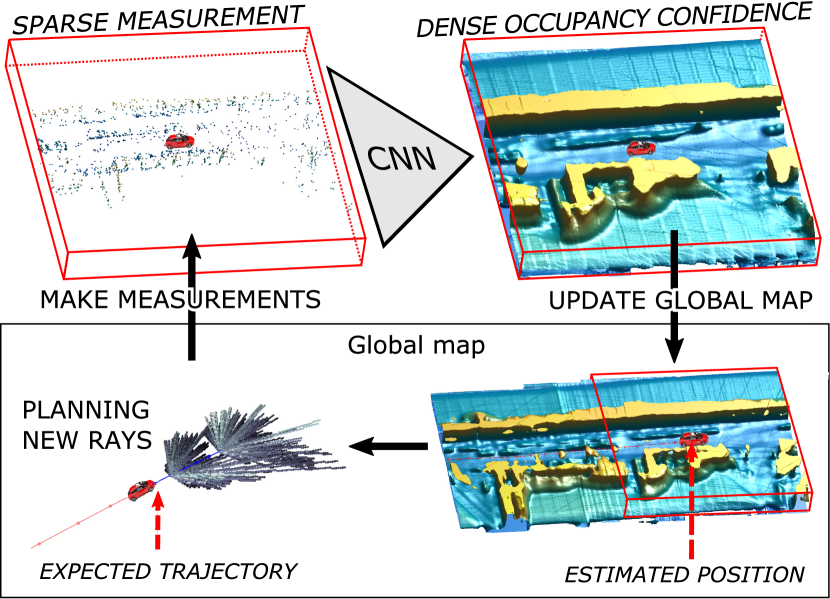
Figure 1: Active 3D mapping with Solid State Lidar. Iteratively learned deep convolutional network reconstructs local dense occupancy map from sparse depth measurements. The local map is registered to a global occupancy map, which in turn serves as an input for the optimization of depth-measuring rays along the expected vehicle trajectory. The dense occupancy maps are visualized as isosurfaces. See https://www.youtube.com/watch?v=KNex0zjeGYE

The main contribution of this paper lies in proposing a computationally tractable approach for very high-dimensional active perception task, which couples learning of the 3D reconstruction with the optimization of depth-measuring rays. Unlike other approaches such as active object detection [6] or segmentation [7], SSL-like reactive control has significantly higher dimensionality of the state-action space, which makes a direct application of unsupervised reinforcement learning [6] prohibitively expensive. Keeping the on-board reactive control in mind, we propose prioritized greedy optimization of depth measuring rays, which in contrast to a naïve greedy algorithm re-evaluates only $1/500$ rays in each iteration. We derive the approximation ratio of the proposed algorithm.

The 3D mapping is handled by an iteratively learned convolution neural network (CNN), as CNNs proved their superior performance in [3, 17]. The iterative learning procedure stems from the fact that both (i) the directions in which the depth should be measured and (ii) the weights of the 3D reconstruction network are unknown. We initialize the learning procedure by selecting depth-measuring rays randomly to learn an initial 3D mapping network which estimates occupancy of each particular voxel. Then, using this network, depth-measuring rays along the expected vehicle trajectory can be planned based on the expected reconstruction (in)accuracy in each voxel. To reduce the training-planning discrepancy, the mapping network is re-learned on optimized sparse measurements and the whole process is iterated until validation error stops decreasing.

2 Previous work

High performance of image-based models is demonstrated in [14], where a CNN pooling results from multiple rendered views outperforms commonly used 3D shape descriptors in object recognition task. Qi et al. [10] compare several volumetric and multi-view network architectures and propose an anisotropic probing kernel to close the performance gap between the two approaches. Our network architecture uses a similar design principle.

Choy et al. [3] proposed a unified approach for single and multi-view 3D object reconstruction which employs a recurrent neural architecture. Despite providing competitive results in the object reconstruction domain, the architecture is not suitable for dealing with high-dimensional outputs due to its high memory requirements and would need significant modifications to train with full-resolution maps which we use. We provide a comparison of this method to ours in Sec. 6.2, in a limited setting.

Model-fitting methods such as [13, 15, 11] rely on a manually-annotated dataset of models and assume that objects can be decomposed into a predefined set of parts. Besides that these methods are suited mostly for man-made objects of rigid structure, fitting of the models and their parts to the input points is computationally very expensive; e.g., minutes per input for [13, 15]. Decomposition of the scene into plane primitives as in [8] does not scale well with scene size (quadratically due to candidate pairs) and could not most likely deal with the level of sparsity we encounter.

Geometrical and physical reasoning comprising stability of objects in the scene is used by Zheng et al. [18] to improve object segmentation and 3D volumetric recovery. Their assumption of objects being aligned with coordinate axes which seems unrealistic in practice. Moreover, it is not clear how to incorporate learned shape priors for complex real-world objects which were shown to be beneficial for many tasks (e.g., in [9]). Firman et al. [4] use a structured-output regression forest to complete unobserved geometry of tabletop-sized objects. A generative model proposed by Wu et al. [17], termed Deep Belief Network, learns joint probability distribution $p(\mathrm{\mathbf{x}},y)$ of complex 3D shapes $\mathrm{\mathbf{x}}$ across various object categories $y$.

End-to-end learning of stochastic motion control policies for active object and scene categorization is proposed by Jayaraman and Grauman [6]. Their CNN policy successively proposes views to capture with RGB camera to minimize categorization error. The authors use a look-ahead error as an unsupervised regularizer on the classification objective. Andreopoulos et al. [2] solve the problem of an active search for an object in a 3D environment. While they minimize the classification error of a single yet apriori unknown voxel containing the searched object, we minimize the expected reconstruction error of all voxels. Also, their action space is significantly smaller than ours because they consider only local viewpoint changes at the next position while the SSL planning chooses from tens of thousands of rays over a longer horizon.

3 Overview of the active 3D mapping

We assume that the vehicle follows a known path consisting of $L$ discrete positions and a depth measuring device (SSL) can capture at most $K$ rays at each position. The set of rays to be captured at position $l$ is denoted $J_{l}$.

We denote $\mathrm{\mathbf{Y}}$ the global ground-truth occupancy map, $\hat{\mathrm{\mathbf{Y}}}$ its estimate, and $\mathrm{\mathbf{X}}$ the map of the sparse measurements. All these map share common global reference frame corresponding to the first position in the path. For each of these maps there are local counterparts $\mathrm{\mathbf{y}}_{l},\hat{\mathrm{\mathbf{y}}}_{l}$, and $\mathrm{\mathbf{x}}_{l}$, respectively. Local maps corresponding to position $l$ all share a common reference frame which is aligned with the sensor and captures its local neighborhood. The global ground-truth map $\mathrm{\mathbf{Y}}$ is used to synthesize sensor measurements $\mathrm{\mathbf{x}}_{l}$ and to generate local ground-truth maps $\mathrm{\mathbf{y}}_{l}$ for training.

The active mapping pipeline, consisting of a measure-reconstruct-plan loop, is depicted in Fig. 1 and detailed in Alg. 1.

1:Initialize position $l\leftarrow 0$ and select depth-measuring rays randomly.

2:Measure depth in the directions selected for position $l$ and update global sparse measurements $\mathrm{\mathbf{X}}$ and dense reconstruction $\hat{\mathrm{\mathbf{Y}}}$ with these measurements.

3:Obtain local measurements $\mathrm{\mathbf{x}}_{l}$ by interpolating $\mathrm{\mathbf{X}}$.

4:Compute local occupancy confidence $\hat{\mathrm{\mathbf{y}}}_{l}=\mathrm{\mathbf{h}}_{\theta}(\mathrm{\mathbf{x}}_{l})$ using the mapping network $\mathrm{\mathbf{h}}_{\theta}$.

5:Update global occupancy confidence $\hat{\mathrm{\mathbf{Y}}}\leftarrow\hat{\mathrm{\mathbf{Y}}}+\hat{\mathrm{\mathbf{y}}}_{l}$.

6:Plan depth-measuring rays along the expected vehicle trajectory over horizon $L$ given reconstruction $\hat{\mathrm{\mathbf{Y}}}$.

7:Repeat from line 2 for next position $l\leftarrow l+1$.

Algorithm 1 Active mapping

Neglecting sensor noise, the set of depth-measuring rays obtained from the planning, the measurements $\mathrm{\mathbf{x}}_{l}$, and the resulting reconstruction $\hat{\mathrm{\mathbf{Y}}}$ can all be seen as a deterministic function of mapping parameters $\theta$ and $\mathrm{\mathbf{Y}}$. If we assume that that ground-truth maps $\mathrm{\mathbf{Y}}$ come from a probability distribution, both learning of $\theta$ and planning of the depth-measuring rays approximately minimize common objective

$$\mathbb{E}_{\mathrm{\mathbf{Y}}}\{\mathcal{L}(\mathrm{\mathbf{Y}},\hat{\mathrm{\mathbf{Y}}}(\theta,\mathrm{\mathbf{Y}}))\},$$ (1)

where $\mathcal{L}(\mathrm{\mathbf{Y}},\hat{\mathrm{\mathbf{Y}}})=\sum_{i}w_{i}\log(1+\exp(-Y_{i}\hat{Y}_{i}))$ is the weighted logistic loss, $Y_{i}\in\{-1,1\}$ and $\hat{Y}_{i}\in\mathbb{R}$ denote the elements of $\mathrm{\mathbf{Y}}$ and $\hat{\mathrm{\mathbf{Y}}}$, respectively, corresponding to voxel $i$. In learning, $w_{i}\geq 0$ are used to balance the two classes, empty with $Y_{i}=-1$ and occupied with $Y_{i}=1$, and to ignore the voxels with unknown occupancy. We assume independence of measurements and use, for corresponding voxels $i$, additive updates of the occupancy confidence $\hat{Y}_{i}\leftarrow\hat{Y}_{i}+h_{i}(\mathrm{\mathbf{x}}_{l})$ with $h_{i}(\mathrm{\mathbf{x}}_{l})\approx\log(\mathrm{Pr}(Y_{i}=1|\mathrm{\mathbf{x}}_{l})/\mathrm{Pr}(Y_{i}=-1|\mathrm{\mathbf{x}}_{l}))$. $\mathrm{Pr}(Y_{i}=1|\mathrm{\mathbf{x}}_{l})$ denotes the conditional probability of voxel $i$ being occupied given measurements $\mathrm{\mathbf{x}}_{l}$ and $\sigma(\hat{Y}_{i})=1/(1+e^{-\hat{Y}_{i}})$ is its current estimate.

4 Learning of 3D mapping network

The learning is defined as approximate minimization of Equation 1. Since (i) the result of planning $\mathrm{\mathbf{x}}_{l}\left(\theta,\mathrm{\mathbf{Y}}\right)$ is not differentiable with respect to $\theta$ and (ii) we want to reduce variability of training data, we locally approximate the criterion around a point $\theta^{0}$ as

$$\mathbb{E}_{\mathrm{\mathbf{Y}}}\{\sum_{l}\mathcal{L}(\mathrm{\mathbf{y}}_{l},\mathrm{\mathbf{h}}_{\theta}(\mathrm{\mathbf{x}}_{l}(\theta^{0},\mathrm{\mathbf{Y}})))\}$$ (2)

by fixing the result of planning in $\mathrm{\mathbf{x}}_{l}(\theta^{0},\mathrm{\mathbf{Y}})$. We also introduce a canonical frame by using the local maps instead of the global ones, which helps the mapping network to capture local regularities. The learning then becomes the following iterative optimization

$$\theta^{t}=\arg\min_{\theta}\mathbb{E}_{\mathrm{\mathbf{Y}}}\{\sum_{l}\mathcal{L}(\mathrm{\mathbf{y}}_{l},\mathrm{\mathbf{h}}_{\theta}(\mathrm{\mathbf{x}}_{l}(\theta^{t-1},\mathrm{\mathbf{Y}})))\},$$ (3)

where minimization in each iteration is tackled by Stochastic Gradient Descent. Learning is summarized in Alg. 2.

1:Initialize $t\leftarrow 0$ and obtain dataset $D_{0}=\{(\mathrm{\mathbf{x}}_{l},\mathrm{\mathbf{y}}_{l})\}_{l}$ by running the pipeline with the rays being selected randomly, instead of using the planner.

2:Train the mapping network on $D_{t}$ to obtain $\mathrm{\mathbf{h}}_{\theta^{t}}$ with parameters $\theta^{t}$.

3:Obtain $D_{t+1}=\{(\mathrm{\mathbf{x}}_{l}(\theta^{t},\mathrm{\mathbf{Y}}),\mathrm{\mathbf{y}}_{l})\}_{l}$ by running Alg. 1 and using $\mathrm{\mathbf{h}}_{\theta^{t}}$ for mapping.

4:Set $t\leftarrow t+1$ and repeat from line 2 until validation error stops decreasing.

Algorithm 2 Learning of active mapping

Note, that in order to achieve (i) local optimality of the criterion and (ii) statistical consistency of the learning process (i.e., that the training distribution of sparse measurements $\mathrm{\mathbf{x}}_{l}$ corresponds to the one obtained by planning), one would have to find a fixed point of Equation 3. Since there are no guarantees that any fixed point exists, we instead iterate the minimization until validation error is decreasing.

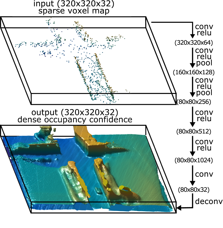
Figure 2: Architecture of the mapping network. Top: An example input with sparse measurements, showing only the occupied voxels. Bottom: The corresponding reconstructed dense occupancy confidence after thresholding. Right: Schema of the network architecture, composed from the convolutional layers (denoted conv), linear rectifier units (relu), pooling layers (pool), and upsampling layers (deconv).

The mapping network consists of 6 convolutional layers with $5\times 5$ kernels followed by linear rectifier units (element-wise $\max\{x,0\}$) and, in 2 cases, by max pooling layers with $2\times 2$ kernels and stride $2$, see Fig. 2. In the end, there is an fourfold upsampling layer so that the output has same size as input. The network was implemented in MatConvNet [16].

5 Planning of depth measuring rays

Planning at position $l$ searches for a set of rays $J$, which approximately minimizes the expected logistic loss $\mathcal{L}(\mathrm{\mathbf{Y}},\mathrm{\mathbf{h}}_{\theta^{t}}(\mathrm{\mathbf{x}}_{l+L}))$ between ground truth map $\mathrm{\mathbf{Y}}$ and reconstruction obtained from sparse measurements $\mathrm{\mathbf{x}}_{l+L}$ at the horizon $L$. The result of planning is the set of rays $J$, which will provide measurements for a sparse set of voxels. This set of voxels is referred to as covered by $J$ and denoted as $C(J)$. While the mapping network is trained offline on the ground-truth maps, the planning have to search the subset of rays online without any explicit knowledge of the ground-truth occupancy $\mathrm{\mathbf{Y}}$. Since it is not clear how to directly quantify the impact of measuring a subset of voxels on the reconstruction $\mathrm{\mathbf{h}}_{\theta^{t}}(\mathrm{\mathbf{x}}_{l+L})$, we introduce simplified reconstruction model $\hat{\mathrm{\mathbf{h}}}(J,\hat{\mathrm{\mathbf{Y}}})$, which predicts the loss based on currently available map $\hat{\mathrm{\mathbf{Y}}}$. This model conservatively assumes that the reconstruction in covered voxels $i\in C(J)$ is correct (i.e. $\mathcal{L}\big{(}Y_{i},\hat{h}_{i}(J,\hat{\mathrm{\mathbf{Y}}})\big{)}=0$) and reconstruction of not covered voxels $i\notin C(J)$ does not change (i.e. $\mathcal{L}\big{(}Y_{i},\hat{h}_{i}(J,\hat{\mathrm{\mathbf{Y}}})\big{)}=\mathcal{L}(Y_{i},\hat{Y}_{i})$). Given this reconstruction model, the expected loss simplifies to:

$$\mkern-5.0mu\sum_{i}\mathcal{L}\big{(}Y_{i},\hat{h}_{i}(J,\hat{\mathrm{\mathbf{Y}}})\big{)}=\sum_{i\notin C(J)}\mathcal{L}(Y_{i},\hat{Y}_{i})$$ (4)

Since the ground-truth occupancy of voxels is apriori unknown, neither the voxel-wise loss nor the coverage are known. We model the expected loss in voxel $i$ as

$$\mathcal{L}(Y_{i},\hat{Y}_{i})\approx\mathbb{E}_{Y_{i}\sim\textrm{B}(\sigma(\hat{Y}_{i}))}\mathcal{L}(Y_{i},\hat{Y}_{i})=\mathcal{H}(\textrm{B}(\sigma(\hat{Y}_{i})))=\epsilon_{i},$$ (5)

where $\mathcal{H}(\textrm{B}(p))$ is the entropy of the Bernoulli distribution with parameter $p$, denoting the probability of outcome $1$ from the possible outcomes $\{-1,1\}$. The vector of concatenated losses $\epsilon_{i}$ is denoted $\mathrm{\mathbf{\boldsymbol{\epsilon}}}$.

The length of particular rays is also unknown, therefore coverage $C(J)$ of voxels by particular rays cannot be determined uniquely. Consequently, we introduce probability $p_{ij}$ that voxel $i$ will not be covered by ray $j\in J$. This probability is estimated from currently available map $\hat{\mathrm{\mathbf{Y}}}$ as the product of (i) the probability that the voxels on ray $j$ which lie between voxel $i$ and the sensor are unoccupied and (ii) the probability that at least one of the following voxels or the voxel $i$ itself are occupied. If ray $j$ does not intersect voxel $i$, then $p_{ij}=1$. The vector of probabilities $p_{ij}$ for ray $j$ is denoted $\mathrm{\mathbf{p}}_{j}$. Assuming that rays $J$ are independent measurements, the expected loss is modeled as $\mathrm{\mathbf{\boldsymbol{\epsilon}}}^{\mathsf{T}}\prod_{j\in J}\mathrm{\mathbf{p}}_{j}$.

The planning searches for the set $J=J_{1}\cup\dots\cup J_{L}$ of subsets $J_{1}\dots J_{L}$ of depth-measuring rays for the following $L$ positions, which minimize the expected loss, subject to budget constraints $|J_{1}|\leq K,\dots|J_{L}|\leq K$

$$\mkern-7.0muJ^{*}=\arg\min_{J}\;\mathrm{\mathbf{\boldsymbol{\epsilon}}}^{\mathsf{T}}\prod_{j\in J}\mathrm{\mathbf{p}}_{j},\,\mathrm{s.t.}\ |J_{1}|\leq K,\dots|J_{L}|\leq K,$$ (6)

where $|J_{l}|$ denotes cardinality of the set $J_{l}$.

This is a non-convex combinatorial problem which needs to be solved online repeatedly for millions of potential rays. We tried several convex approximations, however the high-dimensional optimization has been extremely time consuming and the improvement with respect to the significantly faster greedy algorithm was negligible. As a consequence of that, we have decided to use the greedy algorithm. We first introduce its simplified version (Alg. 3) and derive its properties, the significantly faster prioritized greedy algorithm (Alg. 4) is explained later.

We denote the list of available rays at position $l$ as $V_{l}$. At the beginning, the list of all available rays is initialized as follows $V=V_{1}\cup\dots\cup V_{L}$. Alg. 3 successively builds the set of selected rays $J$. In each iteration the best ray $j^{*}$ is selected, added into $J$ and removed from $V$. The position from which the ray $j^{*}$ is chosen is denoted $l^{*}$. If the budget $K$ of $l^{*}$ is reached, all rays from $V_{l^{*}}$ are removed from $V$.

In order to avoid multiplication of all selected rays at each iteration, we introduce the vector $\mathrm{\mathbf{b}}$, which keeps voxel loss. Vector $\mathrm{\mathbf{b}}$ is initialized as $\mathrm{\mathbf{b}}=\mathrm{\mathbf{\boldsymbol{\epsilon}}}$ and whenever ray $j$ is selected, voxel losses are updated as follows $\mathrm{\mathbf{b}}=\mathrm{\mathbf{b}}\odot\mathrm{\mathbf{p}}_{j}$, where $\odot$ denotes element-wise multiplication.

1:Set of available rays $V$ and budget $K$

2:$J\leftarrow\emptyset$ 4.5cm $\triangleright$ Initialization

3:$\mathrm{\mathbf{b}}\leftarrow\mathrm{\mathbf{\boldsymbol{\epsilon}}}$

4:while $\neg(V=\emptyset)$ do

5:    $j^{*}\leftarrow\arg\min_{j\in V}\mathrm{\mathbf{b}}^{\mathsf{T}}\mathrm{\mathbf{p}}_{j}$ 4.5cm $\triangleright$ Add the best ray

6:    $J\leftarrow J\cup j^{*}$

7:    $\mathrm{\mathbf{b}}\leftarrow\mathrm{\mathbf{b}}\odot\mathrm{\mathbf{p}}_{j}$ 4.5cm $\triangleright$ Update voxel costs

8:    $V\leftarrow V\setminus j^{*}$ 4.5cm $\triangleright$ Remove $j^{*}$ from $V$

9:    if $|J_{l^{*}}|=K$ then

10:         $V\leftarrow V\setminus V_{l^{*}}$ 4.5cm $\triangleright$ Close position

11:    end if

12:end while

13:return Set of selected rays $J$

Algorithm 3 Greedy planning

The rest of this section is organized as follows: Section 5.1 shows the upper bound for the approximation ratio of the greedy algorithm. Section 5.2 introduces the prioritized greedy algorithm, which in each iteration needs to re-evaluate the cost function $\mathrm{\mathbf{b}}^{\mathsf{T}}\mathrm{\mathbf{p}}_{j}$ only for a small fraction of rays.

5.1 Approximation ratio of the greedy algorithm

We define the approximation ratio of a minimization algorithm to be $\rho=\frac{f}{{\textsc{opt}}}$, where $f$ is the cost function achieved by the algorithm and opt is the optimal value of the cost function. Given $\rho$, we know that the algorithm provides solution whose value is at most $\rho\ {\textsc{opt}}$. In this section we derive the upper bound of the approximation ratio ${\textsc{UB}}(\rho)$ of Algorithm 3. Figure 3 shows values of ${\textsc{UB}}(\rho)$ for different number of positions $L$.

The greedy algorithm successively selects rays that reduce the cost function the most. To show how cost function differs from opt, an upper bound on the cost function need to be derived. Let us suppose that in the beginning of an arbitrary iteration we have voxel losses given by vector $\mathrm{\mathbf{b}}$, the following lemma states that for arbitrary voxel $i$, there always exists a ray $j$, that reduces the cost function to $\sum_{i}b_{i}(1-\frac{1}{K})+\frac{{\textsc{opt}}}{K}$, where ${\textsc{opt}}=\mathrm{\mathbf{1}}^{\mathsf{T}}\prod_{j=1}^{K}\mathrm{\mathbf{p}}_{j}=\mathrm{\mathbf{1}}^{\mathsf{T}}\mathrm{\mathbf{p}}^{{\textsc{opt}}}$ is the unknown optimum value of the cost function which is achievable by $K$ rays $\mathrm{\mathbf{p}}_{1}\dots\mathrm{\mathbf{p}}_{K}$.

Lemma 5.1.

If for some rays $\prod_{j=1}^{K}p_{ij}=p_{i}^{{\textsc{opt}}}$ then

$$\forall_{\mathrm{\mathbf{0}}\leq\mathrm{\mathbf{b}}\leq\mathrm{\mathbf{1}}}\exists_{j}\sum_{i=1}^{V}p_{ij}b_{i}\leq\sum_{i=1}^{V}b_{i}(1-\frac{1}{K})+\frac{{\textsc{opt}}}{K}$$ (7)

Proof: We know that there is optimal solution consisting from $K$ rays. Without loss of generality we assume that $\prod_{j=1}^{K}p_{ij}=p_{i}^{{\textsc{opt}}}$ holds for first $K$ rays, then

$$\forall_{i}\sum_{j=1}^{K}p_{ij}\leq K-1+p^{{\textsc{opt}}}_{i}.$$ (8)

This holds for an arbitrary positive scaling factor $b_{i}$, therefore

$$\forall_{i}\sum_{j=1}^{K}p_{ij}b_{i}\leq(K-1+p^{{\textsc{opt}}}_{i})b_{i}.$$ (9)

We sum up inequalities over all voxels $i$

$$\sum_{i=1}^{V}\sum_{j=1}^{K}p_{ij}b_{i}\leq\sum_{i=1}^{V}(K-1+p^{{\textsc{opt}}}_{i})b_{i}.$$ (10)

We switch sums in the left hand side of the inequality to obtain addition of $K$ terms as follows

$$\sum_{i=1}^{V}p_{i1}b_{i}+\dots+\sum_{i=1}^{V}p_{iK}b_{i}\leq\sum_{i=1}^{V}(K-1+p^{{\textsc{opt}}}_{i})b_{i}$$ (11)

Hence, we know that at least one of these $K$ terms has to be smaller than or equal to $\frac{1}{K}$ of the right hand side

$$\exists_{j}\sum_{i=1}^{V}p_{ij}b_{i} \leq \frac{1}{K}\sum_{i=1}^{V}(K-1+p^{{\textsc{opt}}}_{i})b_{i}=$$

$$= \sum_{i=1}^{V}b_{i}(1-\frac{1}{K})+\frac{1}{K}\sum_{i=1}^{V}p^{{\textsc{opt}}}_{i}b_{i}\leq$$

$$\leq \sum_{i=1}^{V}b_{i}(1-\frac{1}{K})+\sum_{i=1}^{V}\frac{p^{{\textsc{opt}}}_{i}}{K}=$$

$$= \sum_{i=1}^{V}b_{i}(1-\frac{1}{K})+\frac{{\textsc{opt}}}{K}\hskip 36.98866pt\square$$

Especially, if there is only one position, all optimal $K$ rays $\mathrm{\mathbf{p}}_{1}\dots\mathrm{\mathbf{p}}_{K}$ are either already selected or still available. This assumption allows to derive the following upper bound on the cost function of the greedy algorithm $f^{K}$ after $K$ iterations for $L=1$.

Theorem 5.1.

Upper bound $\mathit{{\textsc{UB}}}(f^{K})\geq f^{K}$ of the greedy algorithm after $K$ iterations is

$$\mathit{{\textsc{UB}}}(f^{K})=E\frac{1}{e}+{\textsc{opt}}\left(1-\frac{1}{e}\right),$$ (13)

where $E=\sum_{i=1}^{V}\epsilon_{i}$ and $e$ is Euler number.

Proof: We prove the upper bound by complete induction. In the beginning no ray is selected, per-voxel loss is $b_{i}^{0}=\epsilon_{i}$ and the value of the cost function $f^{0}=\sum_{i=1}^{V}b_{i}^{0}=E$. Using Lemma 5.1, we know that there exists ray $j$ such that $\sum_{i=1}^{V}p_{ij}b_{i}^{0}\leq\sum_{i=1}^{V}b_{i}^{0}(1-\frac{1}{k})+\frac{{\textsc{opt}}}{K}$, therefore we know that

$$f^{1}=\sum_{i=1}^{V}p_{ij}b_{i}^{0}\leq\sum_{i=1}^{V}b_{i}^{0}\left(1-\frac{1}{K}\right)+\frac{{\textsc{opt}}}{K}=$$

$$=E\left(1-\frac{1}{K}\right)+\frac{{\textsc{opt}}}{K}.$$ (14)

Greedy algorithm continues by updating the per-voxel loss $b_{i}^{1}=b_{i}^{0}p_{ij}$. In the second iteration there are two possible cases: (i) we have either used the optimal ray in the first iteration, then the situation is better and we know there is $(K-1)$ rays which achieves optimum, or (ii) we have not selected the optimal ray in the first iteration, therefore we have still $K$ rays which achieves the optimum. Since the cost function reduction in the latter case gives the upper bound on the cost function reduction in the former one, we assume that there is still $k$ optimal rays available, therefore there exists ray $j$ such that

$$f^{2} = \sum_{i=1}^{V}p_{ij}b_{i}^{1}\leq\sum_{i=1}^{V}b_{i}^{1}\left(1-\frac{1}{k}\right)+\frac{{\textsc{opt}}}{K}\leq$$ (15)

$$\leq E\left(1-\frac{1}{K}\right)^{2}+\frac{{\textsc{opt}}}{K}\left(\left(1-\frac{1}{K}\right)+1\right).$$

We assume that the following holds

$$f^{t-1} \leq E\left(1-\frac{1}{K}\right)^{t-1}+\frac{{\textsc{opt}}}{K}\sum_{u=0}^{t-2}\left(1-\frac{1}{K}\right)^{u}.$$ (16)

and prove the inequality for $f^{t}$. Using the assumption (16) and Lemma 5.1, the following inequalities hold

$$f^{t}\leq\sum_{i=1}^{V}b_{i}^{t-1}\left(1-\frac{1}{K}\right)+\frac{{\textsc{opt}}}{K}\leq$$

$$\leq\left[E\left(1-\frac{1}{K}\right)^{t-1}\!\!\!\!\!\!+\frac{{\textsc{opt}}}{K}\sum_{u=0}^{t-2}\left(1-\frac{1}{K}\right)^{u}\right]\left(1-\frac{1}{K}\right)+\frac{{\textsc{opt}}}{K}$$

$$=E\underbrace{\left(1-\frac{1}{K}\right)^{t}}_{\alpha_{t}^{K}}+{\textsc{opt}}\underbrace{\frac{1}{K}\sum_{u=0}^{t-1}\left(1-\frac{1}{K}\right)^{u}}_{\beta_{t}^{K}}$$ (17)

Since $\alpha_{t}^{K}+\beta_{t}^{K}=1$ and $\alpha_{K}=\left(1-\frac{1}{K}\right)^{K}\leq\frac{1}{e}$, the upper bound for cost function of the greedy algorithm in $K$th iteration is $f^{K}\leq E\frac{1}{e}+{\textsc{opt}}\left(1-\frac{1}{e}\right)$                   $\square$

Theorem 5.1 reveals that the approximation ratio of the greedy algorithm $\rho=\frac{f^{K}}{{\textsc{opt}}}$ after $K$ iterations has following upper bound

$$\rho\leq\frac{{\textsc{opt}}(\frac{E}{{\textsc{opt}}}\frac{1}{e}+\left(1-\frac{1}{e}\right))}{{\textsc{opt}}}\leq\frac{E}{{\textsc{LB}}({\textsc{opt}})e}+\left(1-\frac{1}{e}\right)$$ (18)

We can simply find ${\textsc{LB}}({\textsc{opt}})$ by considering for each voxel the best $K$ rays independently.

So far we have assumed that the greedy algorithm chooses only $K$ rays and that all rays are available in all iterations. Since there are $L$ positions and the greedy algorithm can choose only $K$ rays at each position, some rays may be no longer available when choosing $(K+1)$th ray. In the worst case possible, the rays from the most promising position will become unavailable. Since we have not chosen optimal rays we can no longer achieve opt. Nevertheless, we can still choose from rays which achieve a new optimum.

We introduce $\overline{{\textsc{opt}}}_{v}$ as the optimum achievable after closing $v$ positions. Obviously $\overline{{\textsc{opt}}}_{0}={\textsc{opt}}$. Let us assume that, when the first position is closed we cannot lose more than $R_{1}$, therefore $\overline{{\textsc{opt}}}_{1}={\textsc{opt}}+R_{1}$. Without any additional assumption, $R_{1}$ could be arbitrarily large. We discuss potential assumptions later. Similarly $\overline{{\textsc{opt}}}_{2}={\textsc{opt}}+R_{1}+R_{2}$, and $\overline{{\textsc{opt}}}_{v}={\textsc{opt}}+\sum_{l=1}^{v}R_{l}$. The following theorem states the upper bound for $f^{LK}$ as a function of $\overline{{\textsc{opt}}}_{v}$.

Theorem 5.2.

Upper bound $\mathit{{\textsc{UB}}}(f^{LK})\geq f^{LK}$ of the greedy algorithm after $LK$ iterations is

$$\mathit{{\textsc{UB}}}(f^{LK})=E\frac{1}{e}+\sum_{u=0}^{L-1}\gamma_{u}\overline{{\textsc{opt}}_{u}},$$ (19)

where $\gamma_{u}=\left(1-\sqrt[L]{\frac{1}{e}}\right)\left(\sqrt[L]{\frac{1}{e}}\right)^{L-1-u}$

Proof.

We start from the result (17) shown in the proof of Theorem 5.1. Since there is $LK$ rays achieving optimum $\overline{{\textsc{opt}}_{0}}={\textsc{opt}}$, the cost function $f^{K}$ in $K$th iteration is bounded as follows

$$\mkern-26.0muf^{K}\leq E\underbrace{\left(1-\frac{1}{LK}\right)^{K}}_{\alpha_{K}^{LK}}+\overline{{\textsc{opt}}_{0}}\underbrace{\frac{1}{LK}\sum_{u=0}^{K-1}\left(1-\frac{1}{LK}\right)^{u}}_{\beta_{K}^{LK}}$$ (20)

In the $(K+1)$th iteration, there are two possible cases: (i) rays from some position $l$ become not available and there is $K(L-1)$ rays available which can achieve a new optimum which is not higher than $\overline{{\textsc{opt}}_{1}}$ or (ii) all rays are available and there is still $LK$ rays which achieve $\overline{{\textsc{opt}}}_{0}={\textsc{opt}}$. Noticing that the upper bound is increasing in $\overline{{\textsc{opt}}}_{0}$ and $L$, we can cover both cases by considering there is still $LK$ rays which achieves $\overline{{\textsc{opt}}_{1}}$, therefore

$$f^{K+1}\leq(E\alpha_{K}^{LK}+\overline{{\textsc{opt}}_{0}}\beta_{K}^{LK})(1-\frac{1}{LK})+\frac{\overline{{\textsc{opt}}_{1}}}{LK}=$$

$$\;\;\;\;\;\;\;\;\;=E\alpha_{K+1}^{LK}+\overline{{\textsc{opt}}_{0}}\beta_{K}^{LK}(1-\frac{1}{LK})+\frac{\overline{{\textsc{opt}}_{1}}}{LK}$$ (21)

We can now continue up to the iteration $2K$ in which the upper bound is as follows

$$f^{2K}\leq E\alpha_{2K}^{LK}+\overline{{\textsc{opt}}_{0}}\beta_{K}^{LK}\alpha_{K}^{LK}+\overline{{\textsc{opt}}_{1}}\beta_{K}^{LK}$$ (22)

For $(2K+1)$th iteration the situation is similar as for ${(K+1)}$th iteration. In order to cover both cases, we consider that there is $LK$ rays which achieves $\overline{{\textsc{opt}}_{2}}$ and continue up to the $3k$th iteration, which yields the following upper bound

$$f^{3K} \leq E\alpha_{3K}^{LK}+\overline{{\textsc{opt}}_{0}}\beta_{K}^{LK}\alpha_{2K}^{LK}+$$ (23)

$$+\overline{{\textsc{opt}}_{1}}\beta_{K}^{LK}\alpha_{K}^{LK}+\overline{{\textsc{opt}}_{2}}\beta_{K}^{LK}$$

Finally after $LK$ iterations the upper bound is

$$f^{LK}\leq E\alpha_{LK}^{LK}+\beta_{K}^{LK}\sum_{u=0}^{L-1}\alpha_{(L-1-u)K}^{LK}\overline{{\textsc{opt}}_{u}}\leq$$

$$\leq E\frac{1}{e}+\sum_{u=0}^{L-1}\left(1-\sqrt[L]{\frac{1}{e}}\right)\left(\sqrt[L]{\frac{1}{e}}\right)^{L-1-u}\!\!\!\!\!\!\!\!\!\!\!\!\!\!\!\overline{{\textsc{opt}}_{u}}.$$ (24)

The last inequality stems from the fact that $(\alpha_{K}^{LK})^{L}=\alpha_{LK}^{LK}\leq\frac{1}{e}$ and that $\alpha_{K}^{LK}+\beta_{K}^{LK}=1$. ∎

Finally we derive the upper bound of the approximation ratio $\rho={f^{LK}}/{{\textsc{opt}}}$.

Theorem 5.3.

Upper bound of the approximation ratio is

$$\rho\geq\frac{E}{\mathsf{{\textsc{LB}}}({\textsc{opt}})}\frac{1}{e}+\sum_{u=0}^{L-1}\gamma_{u}\left(1+\frac{\sum_{v=1}^{u}R_{v}}{\small{{\textsc{LB}}({\textsc{opt}})}}\right)$$ (25)

where ${\textsc{LB}}({\textsc{opt}})$ is lower bound of the opt.

Proof:

$$\rho=\frac{f^{LK}}{{\textsc{opt}}}\leq\frac{{\textsc{UB}}(f^{LK})}{{\textsc{opt}}}=\frac{E\frac{1}{e}+\sum_{u=1}^{L}\gamma_{u}\overline{{\textsc{opt}}}_{u}}{{\textsc{opt}}}=$$

$$=\frac{{\textsc{opt}}(\frac{E}{{\textsc{opt}}}\frac{1}{e}+\sum_{u=1}^{L}\gamma_{u}\frac{\overline{{\textsc{opt}}}_{u}}{{\textsc{opt}}})}{{\textsc{opt}}}=$$

$$=\frac{E}{{\textsc{opt}}}\frac{1}{e}+\sum_{u=1}^{L}\gamma_{u}\frac{{\textsc{opt}}+\sum_{v=1}^{u}R_{v}}{{\textsc{opt}}}\leq$$ (26)

$$\leq\frac{E}{{\textsc{LB}}({\textsc{opt}})}\frac{1}{e}+\sum_{u=0}^{L-1}\gamma_{u}\left(1+\frac{\sum_{v=1}^{u}R_{v}}{\small{{\textsc{LB}}({\textsc{opt}})}}\right)\;\;\;\;\;\;\;\;\;\;\;\;\;\;\square$$

The approximation ratio depends on the opt, if ${\textsc{opt}}=0$ then $\rho=\infty$, if ${\textsc{opt}}=E$ then $\rho=1$. If we make an assumption that each position covers only $\frac{1}{L}$ fraction of voxels, then $R_{v}\leq\frac{V}{L}$. Figure 3 shows values of ${\textsc{LB}}(\rho)$ for different ratios of $\frac{{\textsc{opt}}}{E}$ for this case.

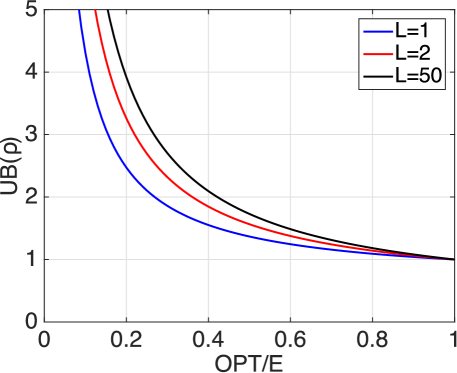
Figure 3: $\text{{{UB}}}(\rho)$ as a function of $\frac{{\textsc{opt}}}{E}$ ratios with $R_{v}\leq\frac{V}{L}$.

5.2 Prioritized greedy planning

In practice we observed a significant speed up of the greedy planning (Alg. 3) by imposing prioritized search for $\arg\min_{j}\mathrm{\mathbf{b}}^{\mathsf{T}}\mathrm{\mathbf{p}}_{j}$. Namely, let us denote $\Delta_{j}^{k}$ the decrease of the expected reconstruction error achieved by selecting ray $j$ in iteration $k$, $\Delta_{j}^{k}=\sum_{i}(b_{i}^{k-1}-b_{i}^{k})=\sum_{i}b_{i}^{k-1}(1-p_{ij}),$ and show that it is non-increasing. For $p_{ij},p_{ij^{\prime}}\in[0,1]$ and $b_{i}^{k-1}\geq 0$ it follows that $b_{i}^{k-1}(1-p_{ij})\geq b_{i}^{k-1}p_{ij^{\prime}}(1-p_{ij})$. Summing the inequalities for all voxels $i$, we get

$$\Delta_{j}^{k}=\sum_{i}b_{i}^{k-1}(1-p_{ij})\geq\sum_{i}b_{i}^{k-1}p_{ij^{\prime}}(1-p_{ij})=\Delta_{j}^{k+1}$$ (27)

for an arbitrary ray $j^{\prime}$ selected in iteration $k$. Note that $\Delta_{j}^{k}\geq\Delta_{j}^{k+a}$ for any $a\geq 1$.

Now, when we search for $j$ maximizing $\Delta_{j}^{k}$ in decreasing order of $\Delta_{j}^{k-a_{j}}$, $a_{j}\geq 1\ \forall j$, we can stop once $\Delta_{j}^{k}>\Delta_{j^{\prime}}^{k-a_{j^{\prime}}}$ for the next ray $j^{\prime}$ because none of the remaining rays can be better than $j$. Moreover, we can take advantage of the fact that all the remaining rays including $j$ remained sorted when updating the priority for the next iteration. The proposed planning is detailed in Alg. 4.

The number of re-evaluations of $\Delta_{j}$ in Alg. 4 was approximately $500\times$ smaller than in Alg. 3. Despite the sorting took about a $1/10$ of the computation time, the prioritized planning was about $30\times$ faster and took $0.3$\mathrm{s}$$ on average using a single-threaded implementation.

1:1cm Set of rays $V=\{1,\ldots,N\}$ at positions $L$, budget $K,$ voxel costs $\mathrm{\mathbf{b}},$ probability vectors $\mathrm{\mathbf{p}}_{j}\ \forall j\in V,$ mapping from ray to position $\lambda\colon V\mapsto L$

2:$J_{l}\leftarrow\emptyset\;\forall{l}\in L$ 4.5cm $\triangleright$ No rays selected

3:$\Delta_{j}\leftarrow\infty\;\forall{j}\in V$ 4.5cm $\triangleright$ Force recompute

4:$S\leftarrow(1,\dots,N)$ 4.5cm $\triangleright$ Sequence of ray indices, $S(n)$ denotes the $n$th element in the sequence, $S(m{:}n)$ the subsequence from the $m$th to the $n$th element.

5:while $S\neq\emptyset$ do

6:    for $n\in(1,\dots,|S|)$ do

7:         $\Delta_{S(n)}\leftarrow\mathrm{\mathbf{b}}^{\mathsf{T}}(\mathrm{\mathbf{1}}-\mathrm{\mathbf{p}}_{S(n)})$

8:         if $n<|S|\land\Delta_{S(n)}\geq\Delta_{S(n+1)}$ then

9:             break

10:         end if

11:    end for

12:    Sort subsequence $S(1:n)$ s.t. $\Delta_{S(n^{\prime})}\geq\Delta_{S(n^{\prime}+1)}$

13:    Merge sorted subsequences $S(1:n-1)$ and $S(n:|S|)$

14:    $j^{*}\leftarrow S(1),l^{*}\leftarrow\lambda(j^{*})$

15:    $J_{l^{*}}\leftarrow J_{l^{*}}\cup\{j^{*}\}$ 4.5cm $\triangleright$ Add the best ray

16:    $\mathrm{\mathbf{b}}\leftarrow\mathrm{\mathbf{b}}\odot\mathrm{\mathbf{p}}_{j^{*}}$ 4.5cm $\triangleright$ Update voxel costs

17:    if $|J_{l^{*}}|=K$ then

18:         $S\leftarrow S\setminus\{j:\lambda(j)=l^{*}\}$ 4.5cm $\triangleright$ Close position

19:    else

20:         $S\leftarrow S\setminus\{j^{*}\}$ 4.5cm $\triangleright$ Remove $j^{*}$ from $S$

21:    end if

22:end while

23:return Selected rays $J_{l}$ at every position $l\in L$

Algorithm 4 Prioritized greedy planning

6 Experiments

Dataset

All experiments were conducted on selected sequences from categories City and Residential from the KITTI dataset [5]. We first brought the point clouds (captured by the Velodyne HDL-64E laser scanner) to a common reference frame using the localization data from the inertial navigation system (OXTS RT 3003 GPS/IMU) and created the ground-truth voxel maps from these. The voxels traced from the sensor origin towards each measured point were updated as empty except for the voxels incident with any of the end points which were updated as occupied for each incident end point. The dynamic objects were mostly removed in the process since the voxels belonging to these objects were also many times updated as empty while moving. All maps used axis-aligned voxels of edge size $0.2\text{\,}\mathrm{m}$.

For generating the sparse measurements, we consider an SSL sensor with the field of view of $120^{\circ}$ horizontally and $90^{\circ}$ vertically discretized in $160\times 120=19200$ directions. At each position, we select $K=200$ rays and ray-trace in these directions until an occupied voxel is hit or the maximum distance of $48$\mathrm{m}$$ is reached. Only the rays which end up hitting an occupied voxel produce valid measurements, as is the case with the time-of-flight sensors. Local maps $\mathrm{\mathbf{x}}_{l}$ and $\mathrm{\mathbf{y}}_{l}$ contain volume of $64$\mathrm{m}$\times 64$\mathrm{m}$\times 6.4$\mathrm{m}$$ discretized into $320\times 320\times 32$ voxels.

6.1 Active 3D mapping

In this experiment, we used $17$ and $3$ sequences from the Residential category for training and validation, respectively, and $13$ sequences from the City category for testing. We evaluate the iterative planning-learning procedure described in Sec. 4. For learning the mapping networks, we used learning rate $\alpha=10^{-3}(1/8)^{\lceil i/10\rceil}$ based on epoch number $i$, batch size $1$, and momentum $0.99$. Networks $\mathrm{\mathbf{h}}_{\theta^{0}},\ldots,\mathrm{\mathbf{h}}_{\theta^{3}}$ were trained for $20$ epochs.

The ROC curves shown in Fig. 4 (left) are computed using ground-truth maps $\mathrm{\mathbf{Y}}$ and predicted global occupancy maps $\hat{\mathrm{\mathbf{Y}}}$. The performance of the $\mathrm{\mathbf{h}}_{\theta^{3}}$ network (denoted Coupled) significantly outperforms the $\mathrm{\mathbf{h}}_{\theta^{3}}$ network (Random), which shows the benefit of the proposed iterative planning-mapping procedure. Examples of reconstructed global occupancy maps are shown in Fig. 5. Note that the valid measurements covered around $3\%$ of the input voxels.

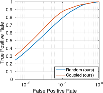
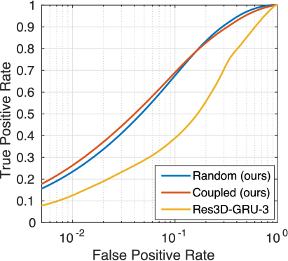
Figure 4: ROC curves of occupancy prediction from active 3D mapping on test sets. Left: Random denotes the global occupancy $\hat{\mathrm{\mathbf{Y}}}$ obtained by using $\mathrm{\mathbf{h}}_{\theta^{0}}$ with random sparse measurements, Coupled the occupancy obtained by using $\mathrm{\mathbf{h}}_{\theta^{3}}$ with the prioritized greedy planning. The voxels which are more than $1$\mathrm{m}$$ from what could possibly be measured are excluded, together with the false positives which can be attributed to discretization error (in 1-voxel distance from an occupied voxel). Right: Random denotes the local occupancy maps $\hat{\mathrm{\mathbf{y}}}_{l}$ obtained by using $\mathrm{\mathbf{h}}_{\theta^{0}}$, Coupled the maps obtained by using $\mathrm{\mathbf{h}}_{\theta^{1}}$, and Res3D-GRU-3 denotes the reconstruction obtained by the network adapted from [3].

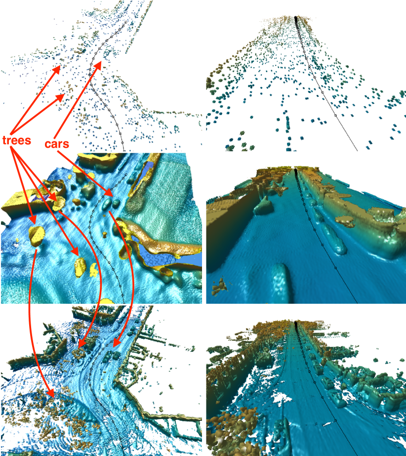
Figure 5: Examples of global map reconstruction. Top: Sparse measurement maps $\mathrm{\mathbf{X}}$. Middle: Reconstructed occupancy maps $\hat{\mathrm{\mathbf{Y}}}$ in form of isosurface. Bottom: Ground-truth maps $\mathrm{\mathbf{Y}}$. The black line denotes trajectory of the car.

6.2 Comparison to a recurrent image-based architecture

We provide a comparison with the image-based reconstruction method of Choy et al. [3]. Namely, we modify their residual Res3D-GRU-3 network to use sparse depth maps of size $160\times 120$ instead of RGB images. The sensor pose corresponding to the last received depth map was used for reconstruction. The number of views were fixed to $5$, with $K=200$ randomly selected depth-measuring rays in each image. For this experiment, we used 20 sequences from the Residential category—18 for training, 1 for validation and 1 for testing. Since the Res3D-GRU-3 architecture is not suited for high-dimensional outputs due to its high memory requirements, we limit the batch size to $1$ and the size of the maps to $128\times 128\times 32$, which corresponds to $16\times 16\times 4$ recurrent units. Our mapping network was trained and tested on voxel maps instead of depth images.

The corresponding ROC curves, computed from local maps $\mathrm{\mathbf{y}}_{l}$ and $\hat{\mathrm{\mathbf{y}}}_{l}$, are shown in Fig. 4 (right). Both $\mathrm{\mathbf{h}}_{\theta^{0}}$ and $\mathrm{\mathbf{h}}_{\theta^{1}}$ networks outperforms the Res3D-GRU-3 network. We attribute this result mostly to the fact that our method is implicitly provided the known trajectory, while the Res3D-GRU-3 network is not. Another reason may be the ray-voxel mapping which is also known implicitly in our case, compared to [3].

7 Conclusions

We have proposed a computationally tractable approach for the very high-dimensional active perception task. The proposed 3D-reconstruction CNN outperforms a state-of-the-art approach by $20\%$ in recall, and it is shown that when learning is coupled with planning, recall increases by additional $8\%$ on the same false positive rate. The proposed prioritized greedy planning algorithm seems to be a promising direction with respect to on-board reactive control since it is about $30\times$ faster and requires only $1/500$ of ray evaluations compared to a naïve greedy solution.

References

• [1] E. Ackerman. Quanergy announces $250 solid-state LIDAR for cars, robots, and more. In IEEE Spectrum, January 2016.
• [2] A. Andreopoulos, S. Hasler, H. Wersing, H. Janssen, J. K. Tsotsos, and E. Körner. Active 3D object localization using a humanoid robot. IEEE Transactions on Robotics, 27(1):47–64, 2011.
• [3] C. B. Choy, D. Xu, J. Gwak, K. Chen, and S. Savarese. 3D-R2N2: A unified approach for single and multi-view 3D object reconstruction. In Computer Vision – ECCV 2016: 14th European Conference on, pages 628–644, Cham, 2016. Springer International Publishing.
• [4] M. Firman, O. M. Aodha, S. Julier, and G. J. Brostow. Structured prediction of unobserved voxels from a single depth image. In 2016 IEEE Conference on Computer Vision and Pattern Recognition (CVPR), pages 5431–5440, June 2016.
• [5] A. Geiger, P. Lenz, C. Stiller, and R. Urtasun. Vision meets robotics: The KITTI dataset. International Journal of Robotics Research, 32(11):1231–1237, Sept. 2013.
• [6] D. Jayaraman and K. Grauman. Look-ahead before you leap: End-to-end active recognition by forecasting the effect of motion. In Computer Vision – ECCV 2016: 14th European Conference on, pages 489–505. Springer International Publishing, Cham, 2016.
• [7] A. K. Mishra, Y. Aloimonos, L. F. Cheong, and A. Kassim. Active visual segmentation. IEEE Transactions on Pattern Analysis and Machine Intelligence, 34(4):639–653, April 2012.
• [8] A. Monszpart, N. Mellado, G. J. Brostow, and N. J. Mitra. RAPter: Rebuilding man-made scenes with regular arrangements of planes. ACM Trans. Graph., 34(4):103:1–103:12, July 2015.
• [9] D. T. Nguyen, B. S. Hua, M. K. Tran, Q. H. Pham, and S. K. Yeung. A field model for repairing 3d shapes. In 2016 IEEE Conference on Computer Vision and Pattern Recognition (CVPR), pages 5676–5684, June 2016.
• [10] C. R. Qi, H. Su, M. Nießner, A. Dai, M. Yan, and L. J. Guibas. Volumetric and multi-view CNNs for object classification on 3D data. In 2016 IEEE Conference on Computer Vision and Pattern Recognition (CVPR), pages 5648–5656, June 2016.
• [11] J. Rock, T. Gupta, J. Thorsen, J. Gwak, D. Shin, and D. Hoiem. Completing 3d object shape from one depth image. In 2015 IEEE Conference on Computer Vision and Pattern Recognition (CVPR), pages 2484–2493, June 2015.
• [12] H. Seifa and X. Hub. Autonomous driving in the iCity—HD maps as a key challenge of the automotive industry. Autonomous Robots, 2(2):159–162, 2016.
• [13] C.-H. Shen, H. Fu, K. Chen, and S.-M. Hu. Structure recovery by part assembly. ACM Trans. Graph., 31(6):180:1–180:11, Nov. 2012.
• [14] H. Su, S. Maji, E. Kalogerakis, and E. Learned-Miller. Multi-view convolutional neural networks for 3D shape recognition. In 2015 IEEE International Conference on Computer Vision (ICCV), pages 945–953, Dec 2015.
• [15] M. Sung, V. G. Kim, R. Angst, and L. Guibas. Data-driven structural priors for shape completion. ACM Trans. Graph., 34(6):175:1–175:11, Oct. 2015.
• [16] A. Vedaldi and K. Lenc. Matconvnet: Convolutional neural networks for matlab. In Proceedings of the 23rd ACM International Conference on Multimedia, MM ’15, pages 689–692, New York, NY, USA, 2015. ACM.
• [17] Z. Wu, S. Song, A. Khosla, F. Yu, L. Zhang, X. Tang, and J. Xiao. 3D ShapeNets: A deep representation for volumetric shapes. In 2015 IEEE Conference on Computer Vision and Pattern Recognition (CVPR), pages 1912–1920, June 2015.
• [18] B. Zheng, Y. Zhao, J. C. Yu, K. Ikeuchi, and S. C. Zhu. Beyond point clouds: Scene understanding by reasoning geometry and physics. In 2013 IEEE Conference on Computer Vision and Pattern Recognition, pages 3127–3134, June 2013.