Excited Boson Stars

Abstract

Axisymmetric rotating radially excited boson stars are analyzed. For several fixed parameter sets, the full sets of solutions are obtained. In contrast to the nodeless boson stars, the radially excited sets of solutions do not exhibit a spiraling behavior. Instead they form a loop, when the boson frequency is varied from its maximal value given by the boson mass to a minimal value and back. Thus for all allowed boundary data of the scalar field at the origin, there are two distinct solutions, except for the endpoints. While one endpoint corresponds to the trivial solution, the other one represents the most compact solution. The energy density and the pressures of the solutions are analyzed. A decomposition of the scalar field into spherical harmonics is performed, and stability considerations are presented.

I Introduction

First obtained almost half a century ago PhysRev.168.1445 ; PhysRev.172.1331 ; PhysRev.187.1767 , boson stars have been studied in many different theoretical and astrophysical contexts (for reviews see e.g. LEE1992251 ; JETZER1992163 ; doi10.1142/S0218271892000057 ; Mielke1997re ; 0264-9381-20-20-201 ; Liebling2012 ). Boson stars arise, when a complex scalar field is coupled to gravity, with the simplest boson stars containing only a mass term but no self-interaction. The inclusion of a repulsive self-interaction allows for more massive stars PhysRevLett.57.2485 , while a sextic potential allows for very massive and highly compact objects, close to the black hole limit PhysRevD.35.3658 .

The astrophysical applications of boson stars range from black hole mimickers with respect to different astrophysical scales in terms of the mass and the accretion rate PhysRevD.80.084023 ; PhysRevD.62.104012 all the way to the description of galactic halos and their lensing properties PhysRevD.66.023503 ; doi:10.1111/j.1365-2966.2006.10330.x . Also multi-state boson stars have been considered, which superpose fundamental and excited boson star solutions to obtain more realistic rotation curves of spiral galaxies PhysRevD.81.044031 ; PhysRevD.82.123535 .

In boson stars, the complex scalar field has a harmonic time dependence with frequency $\omega_{s}$. Besides the fundamental solutions there are also radially excited solutions, where the scalar field has any number of nodes. The properties of spherically symmetric excited boson stars are very similar to those of the fundmental boson stars. In particular, they exist between a maximal value of the boson frequency $\omega_{s}$, corresponding to the mass of the boson field, and a minimal value, depending on the potential and the coupling to gravity. Close to the minimal value of the boson frequency $\omega_{s}$ a spiralling (or oscillating) pattern of the solutions is observed, well-known from other compact objects like neutron stars.

When boson stars are set into rotation, regularity imposes a quantization condition on the scalar field configuration. Consequently, boson stars can only possess angular momenta $J$ which are integer multiples of their particle number $Q$, $J=\hbar mQ$ SCHUNCK1998389 . The properties of rotating boson stars have been investigated widely SCHUNCK1998389 ; PhysRevD.55.6081 ; PhysRevD.56.762 ; Schunck1999 ; MIELKE2000185 ; PhysRevD.72.064002 ; PhysRevD.77.064025 ; PhysRevD.85.024045 . Rotating boson stars follow the pattern of non-rotating boson stars, when the nodeless solutions are considered, independent of the quantum number $m$, or the symmetry of the boson field PhysRevD.72.064002 ; PhysRevD.77.064025 . Interestingly, when rotating sufficiently fast, even ergoregions may arise for boson stars PhysRevD.77.124044 ; PhysRevD.77.064025 .

Motivated by previous studies of multi-state boson stars, which considered non-rotating boson stars only PhysRevD.81.044031 ; PhysRevD.82.123535 , we have undertaken the study of excited rotating boson stars. While we have expected to observe the same pattern for the solutions as seen for the nodeless boson stars, this expectation has not been born out by our investigations. Radially excited rotating boson stars do not exhibit a spiralling or oscillating behavior. Instead for every value of the frequency in the possible range, there are at least two solutions, i.e., the sets of rotating excited boson stars evolve from the maximal frequency to a minimal frequency and then again all the way back to the maximal value.

In this paper we construct numerous sets of excited boson stars and investigate their physical properties. We show that these stars must be constituted by bosons in a superposition of modes. Different mode arrangements allow for equilibrium configurations and therefore more than one solution is found for a fixed value of the field’s radial derivative at the origin.

In Sec. II we present the model and derive the equations we need to solve for. Sec. III contains the description of our numerical methods. In Sec. IV we present and discuss the solutions. We conclude in Sec. V. The appendices contain the field equations and the vierbein components used in the diagonalization of the energy momentum tensor. The metric signature is taken to be $(-,+,+,+)$, Greek indices represent coordinate indices, while Latin indices are used for the vierbein basis. We use geometrical units such that $c=\hbar=8\pi G=1$.

II Model

II.1 Action, Metric and Ansatz

We consider a self-interacting complex scalar field that is minimally coupled to gravity,

$$S=\int\left[\frac{R}{2}-\frac{1}{2}g^{\mu\nu}\left(\Phi_{,\mu}\Phi^{*}_{,\nu}+\Phi_{,\nu}\Phi^{*}_{,\mu}\right)-U\left(\lvert\Phi\rvert\right)\right]\sqrt{-g}d^{4}x,$$ (1)

where $R$ is the curvature scalar, $\Phi$ is the complex scalar field, $U$ is the self-interaction potential, and we employ the compact notation $\Phi_{,\mu}\equiv\partial_{\mu}\Phi$.

To obtain stationary axisymmetric solutions of rotating boson stars, we adopt the quasi-isotropic Lewis-Papapetrou metric in adapted spherical coordinates $(t,r,\theta,\varphi)$. The line element then reads

$$ds^{2}=-fdt^{2}+\frac{l}{f}\left[g\left(dr^{2}+r^{2}d\theta^{2}\right)+r^{2}\sin^{2}\theta\left(d\varphi-\frac{\omega}{r}dt\right)^{2}\right].$$ (2)

This line element contains four scalar functions, namely $f$, $l$, $g$ and $\omega$. For axisymmetric solutions these metric coefficients must be functions of the radial coordinate $r$ and the polar angle $\theta$, only. The spacetime then possesses two Killing vector fields,

$$\xi=\partial_{t},\qquad\eta=\partial_{\varphi}.$$ (3)

Although the boson field is complex, all of the terms in the action are real and functions of $r$ and $\theta$ alone. Therefore, any dependence on the coordinates $t$ and $\varphi$ is included in a phase factor. This results in the ansatz Schunck1996

$$\Phi(t,r,\theta,\varphi)=\phi(r,\theta)e^{i\omega_{s}t+im\varphi},$$ (4)

where $\phi(r,\theta)$ is a real function, and $\omega_{s}$ is the frequency of the boson field, which is also a real number. The identification $\Phi(\varphi)=\Phi(\varphi+2\pi)$ requires $m$ to be an integer number, which may be considered as the field’s rotational quantum number.

The Lagrangian density is invariant under a global $U(1)$ phase transformation $\Phi\rightarrow\Phi e^{i\alpha}$, leading to a conserved current

$$j^{\mu}=-i(\Phi^{\ast}\partial^{\mu}\Phi-\Phi\partial^{\mu}\Phi^{\ast}),\qquad\nabla_{\mu}j^{\mu}=0.$$ (5)

II.2 Potential

In this work, the boson star is a gravitationally bound system of massive interacting bosons described by the complex scalar field $\Phi$. The sixtic potential

$$U\left(\lvert\Phi\rvert\right) =\lambda\Phi^{\ast}\Phi\left[\left(\Phi^{\ast}\Phi\right)^{2}-a\Phi^{\ast}\Phi+b\right]$$

$$=\lambda\phi^{2}\left(\phi^{4}-a\phi^{2}+b\right),$$ (6)

was first proposed as a mechanism for geons to mimic nonlinear spinor fields PhysRevD.20.1303 ; PhysRevD.24.2111 . Friedberg, Lee and Pang then considered non-rotating bosonic nontopological solitons in the presence of gravity, i.e., spherically symmetric boson stars Friedberg:1986tq ; LEE1992251 . A systematic study of nodeless rotating boson stars governed by this potential was performed in PhysRevD.72.064002 ; PhysRevD.77.064025 .

The stability of the boson stars with a sextic potential was investigated via catastrophe theory for spherically symmetric solutions PhysRevD.43.3895 and rotating solutions PhysRevD.85.024045 . The sextic potential is shown in Fig. 1, where we see that its parameters can be chosen in such a manner that it features a local minimum at a finite value of $\phi$, besides the global one at $\phi=0$. From the quadratic term of the potential we read off the boson mass, $m_{b}=\sqrt{\lambda b}$.

Figure 1: The potential $U(\phi)$ for $\lambda=1$, $a=2$, $b=1.1$. Note the global minimum at the origin and a local minimum around $\phi=0.97$.

Bound solutions exist only for a limited range of the frequency $\omega_{s}$. The lower bound depends on the strength of the gravitational coupling, on the potential parameters, and on the character of the solution. In contrast, the upper bound depends on the boson mass alone Friedberg:1986tq ; PhysRevD.66.085003 ; PhysRevD.72.064002

$$\omega_{s}^{2}<\omega_{max}^{2}\equiv\frac{1}{2}\frac{\partial^{2}U\left(\phi\right)}{\partial\phi^{2}}\rvert_{\phi=0}=\lambda b.$$ (7)

Localized solutions can (in principle) be found for any value of $\omega_{s}$ arbitrarily close to $\omega_{max}$, but at the equality the only possible solution is the trivial one. This holds both for solitons in Minkowski space and boson stars in an asymptotically flat spacetime.

II.3 Equations

Variation of the action (1) with respect to the metric yields the Einstein field equations

$$R_{\mu\nu}-\frac{1}{2}Rg_{\mu\nu}=T_{\mu\nu},$$ (8)

where the energy-momentum tensor $T_{\mu\nu}$ is given by

$$T_{\mu\nu} =g_{\mu\nu}\mathcal{L}_{\Phi}-2\frac{\partial L_{\Phi}}{\partial g^{\mu\nu}}$$

$$=-g_{\mu\nu}\left[\frac{1}{2}g^{\rho\tau}\left(\Phi^{\ast}_{,\rho}\Phi_{,\tau}+\Phi^{\ast}_{,\tau}\Phi_{,\rho}\right)+U\left(\lvert\Phi\rvert\right)\right]+\left(\Phi^{\ast}_{,\mu}\Phi_{,\nu}+\Phi^{\ast}_{,\nu}\Phi_{,\mu}\right).$$ (9)

From the above equations it is clear that one can rescale the field $\phi$ with a parameter to be varied. For instance,

$$\kappa T_{\mu\nu}\left(\hat{\phi}\right)=T_{\mu\nu}\left(\phi\right),\qquad\hat{\phi}\equiv\frac{\phi}{\sqrt{\kappa}},$$ (10)

and $\kappa$ is now a free parameter that takes different values to designate either a different gravitational coupling strength or different parameters of the potential $U$. The field equations (8) then take the more general form

$$R_{\mu\nu}-\frac{1}{2}Rg_{\mu\nu}=\kappa T_{\mu\nu}.$$ (11)

Variation with respect to the field gives rise to the Einstein-Klein-Gordon equation

$$\left(\Box-\frac{\partial U}{\partial\lvert\Phi\rvert^{2}}\right)\Phi=0,$$ (12)

where $\Box$ is the covariant D’Alembert differential operator.

II.4 Boundary Conditions

The Einstein field equations (11) give four independent coupled second order elliptic partial differential equations (PDEs) for the metric functions, which can be put in a diagonal form, such that they assume the canonical form of elliptic PDEs with no terms with $\partial^{2}_{r\theta}$ occurring (see Appendix A). These equations together with eq. (12) for the boson field must all be solved simultaneously.

In order to do so we are required to establish boundary conditions for all five functions, that guarantee globally regular bounded solutions. Because of the ansatz (4) adopted for the scalar field and the quadratic dependence of its Lagrangian density $\mathcal{L}_{\Phi}=\mathcal{L}_{\Phi}\left(\Phi^{\ast}\Phi\right)$, the scalar field can have either even or odd parity with respect to reflections on the equatorial plane. Due to this symmetry, the angular domain is reduced to $\theta\in\left[0,\pi/2\right]$. In this work we will analyze only even parity solutions.

For regularity at the origin we demand the conditions

$$\partial_{r}f\rvert_{r=0}=0,\qquad\partial_{r}l\rvert_{r=0}=0,\qquad g\rvert_{r=0}=1,\qquad\omega\rvert_{r=0}=0,\qquad\phi\rvert_{r=0}=0.$$ (13)

In contrast to the non-rotating case, where the scalar field takes a constant value at the origin, rotation induces a singular point at the origin which is regular only if the scalar field vanishes at this point, as seen in eq. (A). This creates a profound change for the scalar field, which assumes a torus-like shape, analogous to the hydrogen wave function, when the magnetic quantum number is different from zero. Near the origin, the scalar field for the rotating boson star has the following expansion

$$\phi(r,\theta)=\phi_{0}r^{m}\sin^{m}\theta,\ \ \ \ \left.\frac{\partial^{m}\phi}{\partial r^{m}}\right|_{\pi/2}=m!\phi_{0}.$$ (14)

The solutions of boson stars will then be parameterized by the value $\phi_{0}$ for rotating and non-rotating boson stars alike.

The gravitationally bound solutions are required to approach asymptotically the Minkowski spacetime. The boundary conditions at infinity read

$$f\rvert_{r\rightarrow\infty}=1,\qquad l\rvert_{r\rightarrow\infty}=1,\qquad g\rvert_{r\rightarrow\infty}=1,\qquad\omega\rvert_{r\rightarrow\infty}=0,\qquad\phi\rvert_{r\rightarrow\infty}=0.$$ (15)

Along the symmetry axis the boundary conditions are given by

$$\partial_{\theta}f\rvert_{\theta=0}=0,\qquad\partial_{\theta}l\rvert_{\theta=0}=0,\qquad g\rvert_{\theta=0}=1,\qquad\partial_{\theta}\omega\rvert_{\theta=0}=0,\qquad\phi\rvert_{\theta=0}=0,$$ (16)

and in the equatorial plane by

$$\partial_{\theta}f\rvert_{\theta=\pi/2}=0,\qquad\partial_{\theta}l\rvert_{\theta=\pi/2}=0,\qquad\partial_{\theta}g\rvert_{\theta=\pi/2}=0,\qquad\partial_{\theta}\omega\rvert_{\theta=\pi/2}=0,\qquad\partial_{\theta}\phi\rvert_{\theta=\pi/2}=0.$$ (17)

The elementary flatness condition

$$\frac{X_{,\mu}X^{,\mu}}{4X}=1,\qquad X=\eta^{\mu}\eta_{\mu},$$ (18)

requires

$$g\rvert_{\theta=0}=g\rvert_{\theta=\pi}=1.$$ (19)

II.5 Conserved Quantities

In a stationary asymptotically flat spacetime, the Komar integrals provide a way to calculate the global charges associated with the Killing vectors. The mass

$$M=2\int_{\Sigma}R_{\mu\nu}n^{\mu}\xi^{\nu}dV,$$ (20)

and the angular momentum

$$J=-\int_{\Sigma}R_{\mu\nu}n^{\mu}\eta^{\nu}dV,$$ (21)

are then obtained from an integral bounded at spatial infinity. Here, $R_{\mu\nu}$ is the Ricci tensor, $\Sigma$ is a spacelike asymptotically flat hypersurface, $n^{\mu}$ is the a vector normal to $\Sigma$ with $n^{\mu}n_{\mu}=-1$. The metric (2) implies that $n^{\mu}=(\xi^{\mu}+\eta^{\mu}\omega/r)/\sqrt{f}$. Substituting the Ricci tensor by the energy-momentum using eq. (11), and noticing that the volume element is $dV=\sqrt{-g/f}drd\theta d\varphi$ one arrives at

$$M=\int(2T^{t}_{t}-T)\sqrt{-g}drd\theta d\varphi,$$ (22)

and

$$J=-\int T^{t}_{\varphi}\sqrt{-g}drd\theta d\varphi.$$ (23)

The mass and angular momentum, being global observables measured at infinity, can also be obtained directly from the asymptotic expansion of the solutions PhysRevLett.86.3704 ,

$$M=\frac{1}{2}\lim_{r\rightarrow\infty}r^{2}\partial_{r}f,\qquad J=\frac{1}{2}\lim_{r\rightarrow\infty}r^{2}\omega.$$ (24)

The Noether charge, associated with the particle number $Q$ of the solutions can be calculated by integrating the projection of the conserved current eq. (5) onto the future directed hypersurface normal $n^{\mu}$ over the whole space,

$$Q =\int_{\Sigma}j_{\mu}n^{\mu}dV$$

$$=\int\frac{2\phi^{2}}{f}\left(\omega_{s}+\frac{m\omega}{r}\right)\sqrt{-g}drd\theta d\varphi.$$ (25)

The integrand of the above equation is simply $-j^{t}\sqrt{-g}$. As noted by Schunck and Mielke Schunck1996 , $T^{t}_{\varphi}=mj^{t}$, then comparison of eq. (II.5) with eq. (23) leads to

$$J=mQ,$$ (26)

and the angular momentum of boson stars is thus quantized.

It is convenient to define a normalization factor for each solution by

$$N^{2}=\int_{\Sigma}\Phi^{\ast}\Phi dV.$$ (27)

III Numerical Approach

The set of five coupled nonlinear elliptic PDEs (A-A) is solved simultaneously, subject to the boundary conditions given above. In order to find the solutions satisfying the appropriate asymptotic behavior, we define a compactified radial coordinate

$$\bar{r}=\frac{r}{1+r},$$ (28)

which goes to one as $r$ goes to infinity.

The equations are solved using the program package FIDISOL Schoenauer:1989 . They are discretized on a nonuniform rectangular grid in $\bar{r}$ and $\theta$, $[0,1]\times[0,\pi/2]$. Then the damped Newton scheme is applied until the desired accuracy is obtained.

Whereas often a known analytic solution of a closely related problem can be successfully used as an initial guess, this is, however, not possible for these boson stars. We therefore proceed by constructing Q-ball solutions for a boson frequency $\omega_{s}$ near $\omega_{\max}$, and use these as initial guesses for the boson stars, since at these values of $\omega_{s}$ we are approaching the trivial solution, where Q-balls and boson stars tend to be very similar.

We here investigate rotating boson star solutions with a first radial excitation. To obtain these we proceed in several steps. Firstly a solution for the non-rotating Q-ball is found using the Runge-Kutta method of 4th order. Then this solution is used to find the equivalent rotating Q-ball as follows, see Fig. 2. As stated above, the rotational quantum number $m$ must be an integer, but in order to get from $m=0$ to $m=1$ one can increase $m$ slowly, starting from zero and passing through unphysical solutions until $m=1$ is reached. Once this value is attained we increase the coupling constant $\kappa$ from zero. This leads us from Q-balls to boson stars. Thus we obtain boson star solutions for different gravitational couplings. All boson stars analyzed here have rotational quantum number $m=1$.

Figure 2: Left: Non-rotating radially excited Q-ball with boson frequency $\omega_{s}=1.01$. Right: Equatorial slice of a rotating radially excited Q-ball with boson frequency $\omega_{s}=1.01$

It is worth to point out that it is difficult to construct solutions with high accuracy at the turning points. However, a good way to guarantee the trustability of a specific solution is to have the asymptotic calculations of $M$ and $J$, eqs. (24), equal the integral ones, eqs. (22) and (23).

IV Solutions

We now discuss the physical properties of the rotating radially excited boson star solutions obtained. We start with their global charges, then address their scalar field distributions, energy densities and pressures, and end with some notes on their stability.

IV.1 Mass and Angular Momentum

To discuss the properties of rotating boson stars, we exhibit in Figs. 3 and 4 the mass $M$ and the angular momentum $J$ of several sets of boson stars versus the boson frequency $\omega_{s}$ for fixed values of the coupling constant $\kappa$. Let us recall, that the particle number $Q$ of rotating boson stars is proportional to their angular momentum, $J=mQ$. Non-rotating boson stars, both the fundamental solutions and the radially excited states, as well as fundamental rotating boson stars, i.e., rotating boson stars without radial nodes, all present a spiraling behavior of the mass $M$ and the angular momentum $J$ versus the boson frequency $\omega_{s}$ LEE1992251 ; PhysRevD.72.064002 . This spiraling behavior is seen in Fig. 3 for the set of fundamental $m=1$ boson star solutions with coupling constant $\kappa=0.05$.

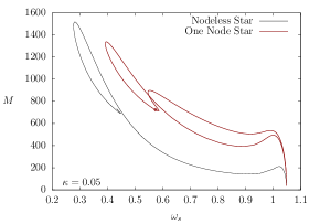
(a)

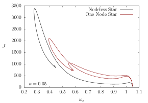
(b)

Figure 3: Left: The mass $M$ of rotating boson stars ($m=1$) with zero nodes (solid line) and with one node (dashed line) versus the boson frequency $\omega_{s}$. Right: The angular momentum $J$ versus the boson frequency $\omega_{s}$ for the same set of solutions. The diamond indicates the radially excited boson star solution with the maximal value of $\phi_{0}$.

For this set of solutions the boson frequency cannot be used any more to characterize the solutions uniquely. Nevertheless the central value of the field $\phi_{0}$ can be used to characterize the non-rotating solutions unless $\kappa$ is very small PhysRevD.85.024045 . Likewise for fundamental rotating boson stars a good parameter choice is usually provided by the $m$-th derivative of the boson field $\phi_{0}=\partial_{r}^{m}\phi(0,\pi/2)/m!$, eq. (14), which incorporates the leading behavior of the scalar field at the origin.

When besides rotation, which induces an angular excitation, further radial excitations are present, the spiraling behavior is no longer present in the set of boson star solutions, as seen in Fig. 3. The curves for the mass and angular momentum of the radially excited rotating boson stars are only similar to those of the rotating boson stars without nodes up to the point, where the onset of the spiral formation occurs for the latter. For the solutions with one radial node we notice, that when the spiral starts forming it soon starts unfolding, and we find at least two solutions for each boson frequency in the allowed domain. Thus the curves of the mass and angular momentum versus the boson frequency form a non-trivial loop, starting from and ending at the trivial solution at $\omega_{\rm max}$.

For a given boson frequency, all solutions of a given set of radially excited rotating boson star solutions (specified by $m$ and $\kappa$), including the intersection point within the loop, represent physically distinct solutions. For the same boson frequency and the same parameters, the radially excited boson stars possess a higher mass and angular momentum than the corresponding nodeless stars (for both branches of the radially excited solutions). Nevertheless, the set of solutions for the excited case is bounded from below by a higher value of $\omega_{\rm min}$ than the nodeless set. Furthermore, the latter presents a higher value for the maximum mass and angular momentum.

In order to find boson star solutions for bosons of different mass the coupling constant $\kappa$ can be varied. The lighter the individual boson is, the more massive will be the corresponding set of boson stars LEE1992251 . The greater the value of $\kappa$, i.e., the higher the boson mass, the greater is also the value of $\omega_{\rm min}$, for which bound solutions exist. Thus the domain of existence of boson star solutions decreases with increasing coupling $\kappa$ as seen in Fig. 4. This feature is observed generically in boson star models. We note, that for the three smaller values of $\kappa$ presented in Fig. 4 some of the solutions contain ergoregions. The onset and termination of the presence of ergoregions there is indicated by small circles.

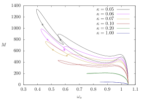
(a)

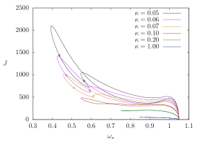
(b)

Figure 4: Left: The mass $M$ of the radially excited boson stars versus the boson frequency $\omega_{s}$ for several values of the coupling $\kappa$. Right: The angular momentum $J$ versus $\omega_{s}$ for the same set of solutions. The circles indicate the onset and termination of the presence of ergoregions.

Independent of the value of the coupling constant $\kappa$, each set of excited rotating boson star solutions forms a loop. Only Q-balls, which are obtained in the limit of vanishing gravity, are special in the sense, that for every value of $\omega_{s}$ there is at most one solution, i.e., one corresponding value of $Q$ and $M$. Therefore, for Q-balls the boson frequency can be used to uniquely parameterize the solutions, which form a two parameter set of solutions $\{m,\omega_{s}\}$ once the behavior of the field is established, namely its radial and angular excitations.

As stated above for spherically symmetric boson stars and rotating boson stars without nodes, the central value of the field $\phi_{0}$ is usually a good parameter to characterize the solutions uniquely. In this case, by increasing the value of $\phi_{0}$, first the spiral is approached and then the solutions wind around the spiral as $\phi_{0}$ keeps increasing. In constrast, radially excited rotating boson stars have an upper limit for $\phi_{0}$, beyond which $\phi_{0}$ decreases again towards zero. This upper limit thus corresponds to a turning point in the $\omega_{s}$ versus $\phi_{0}$ diagram, shown in Fig. 5(a), which also exhibits for comparison the dependence of $\omega_{s}$ versus $\phi_{0}$ for the respective set of nodeless rotating boson stars.

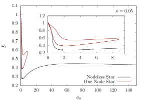
(a)

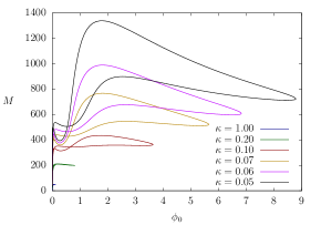
(b)

Figure 5: Left: The boson frequency $\omega_{s}$ versus the value $\phi_{0}$, characterizing the boson field at the origin, for the set of fundamental rotating boson star solutions and those with one nodal excitation for $\kappa=0.05$ and $m=1$. Right: The mass $M$ versus $\phi_{0}$ for the rotating radially excited boson stars for $m=1$ and several values of $\kappa$.

Thus, in the case of rotating radially excited boson stars for every value of $\phi_{0}$ there are two equilibrium configurations. This does not constitute an ill-posed problem, however, because for each pair of solutions with the same value of $\phi_{0}$ for the boson field, the boundary data of the metric functions are different. We also note that at the turning point, i.e., at the maximal value of $\phi_{0}$, there is only a single solution. Likewise, the two branches converge to the trivial solution, when the value of $\phi_{0}$ tends to zero at the maximal value of the boson frequency.

This means that, although we can parameterize the solutions of such a set point by point in a non-trivial way, there is no physical quantity associated with the solutions that could be used as a parameter to characterize the solutions uniquely. We will therefore characterize the solutions by the two branches of this diagram, which we will simply refer to as upper and lower branch (see section IV.5). The triangles in Fig. 5(a) indicate the maximum mass solutions, and occur for the same value $\phi_{0}$ of the boson field. Fig. 5(b) shows how the mass $M$ varies with $\phi_{0}$ for several values of the coupling $\kappa$. Interestingly, when the coupling $\kappa$ is sufficiently small, the maximum mass of a given set is found to reside at $\phi_{0}\sim 1.77$. When the coupling is large, however, the equilibrium configurations are limited by an upper bound of $\phi_{0}$ below that value.

The normalization factor $N$, eq. (27), can be used to normalize the mass and the angular momentum/charge (recall $J=Q$), $\tilde{M}=M/N^{2}$ and $\tilde{Q}=Q/N^{2}$, shown in Fig. 6. The figure shows precisely two branches for each quantity, $\tilde{M}$ and $\tilde{Q}$, which do not intersect themselves, in contrast to the branches of the mass $M$ shown in Fig. 5(a). Note, that the normalized charge attains its maximum just to the left of the turning point.

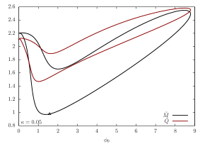
Figure 6: Normalized mass $\tilde{M}$ and charge $\tilde{Q}$ versus the value $\phi_{0}$, characterizing the boson field at the origin, for the set of rotating radially excited solutions for $\kappa=0.05$ and $m=1$. The triangle indicates the maximum mass solution.

IV.2 Boson Field Distribution and Charge Ratio

Let us now focus on the set of rotating radially excited solutions (one node, $m=1$) for coupling constant $\kappa=0.05$. We then demonstrate, that boson star solutions with the same value of $\phi_{0}$ can nevertheless be very different. To this end we exhibit in Fig. 7 the distribution of the boson field, as given by the square of its absolute value $\Phi^{*}\Phi=\phi^{2}$, for two pairs of solutions with very similar boundary conditions. Thus the solutions of each pair correspond to solutions on the upper and lower branch, located almost directly above each other in Figs. 5 and 6.

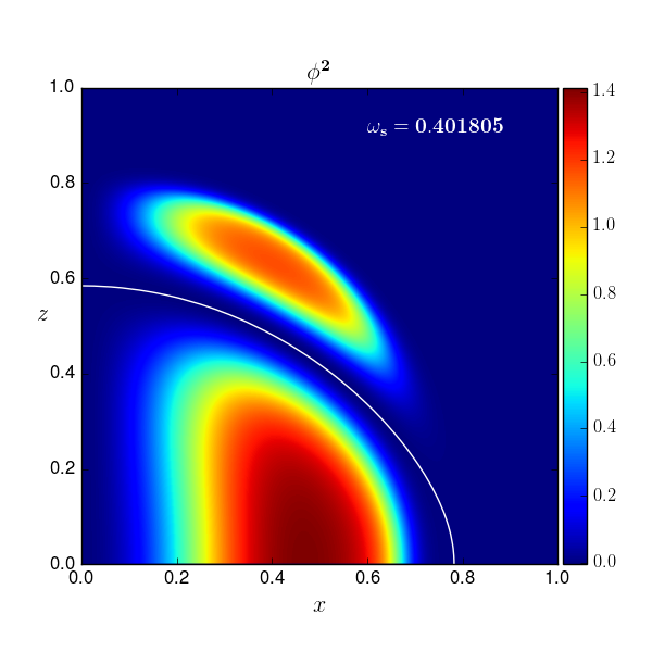
(a) Lower branch, $\phi_{0}=3.08316$

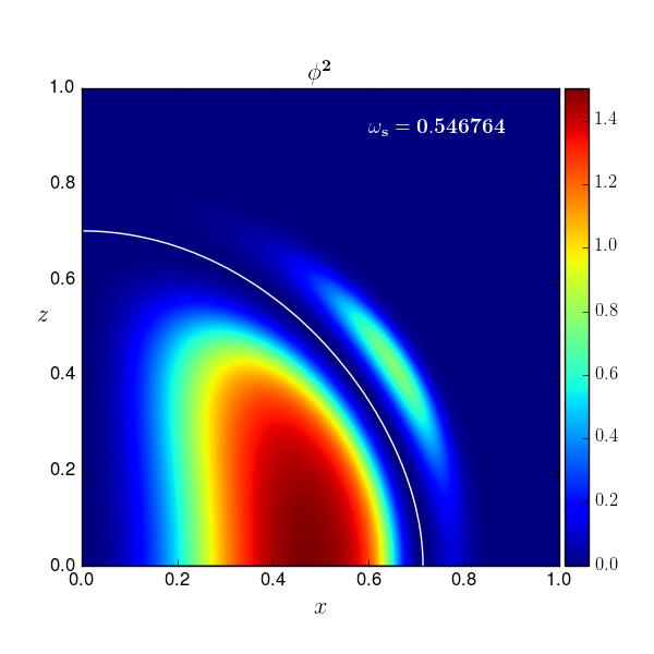
(b) Upper branch, $\phi_{0}=3.07778$

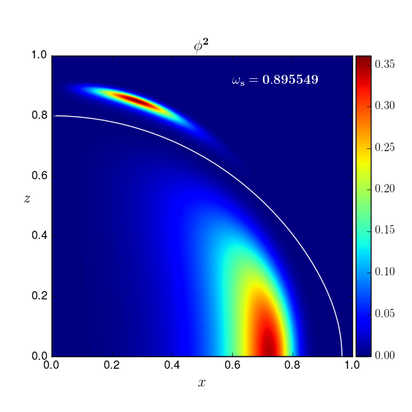
(c) Lower branch, $\phi_{0}=0.251513$

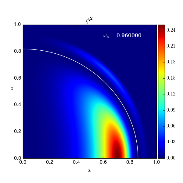
(d) Upper branch, $\phi_{0}=0.258202$

Figure 7: The distribution of the boson field given by the square of its absolute value $\phi^{2}$ on the $xz$-plane, where $z$ is the rotation axis and $x$ is an axis of the equatorial plane, for rotating radially excited solutions (one node, $m=1$, $\kappa=0.05$). The white curve represents the location of the node. Upper panels: Solutions with similar values of $\phi_{0}$ near the turning point. Lower panels: Solutions with similar values of $\phi_{0}$ for smaller $\phi_{0}$.

A rotating radially excited boson star with one node can be thought of a system with two distinct shells. The inner shell always corresponds to values of $\phi>0$ and the outer one to values of $\phi<0$. Although the inner shell is always centered in the equatorial plane, the outer shell enjoys more freedom to center itself at different values of the polar angle $\theta$. For the solutions on the lower branch, the outer shell tends to have its maximum located closer to the rotational axis, i.e., for higher values of $\theta$, than for solutions on the upper branch. Hence we note a higher eccentricity of the nodal curve, represented in Fig. 7 by a white line, for the solutions on the lower branch. The ratio between the negative minimum value of the field and the positive maximum value of the field is overall higher on the upper branch and far from the turning point. Fig. 8 presents for the same set of boson stars the solution at the turning point, where $\phi_{0}$ assumes its maximum value. We note that for this solution the nodal line is at a smaller distance from the origin than for the two solutions close to it, exhibited in Fig. 7.

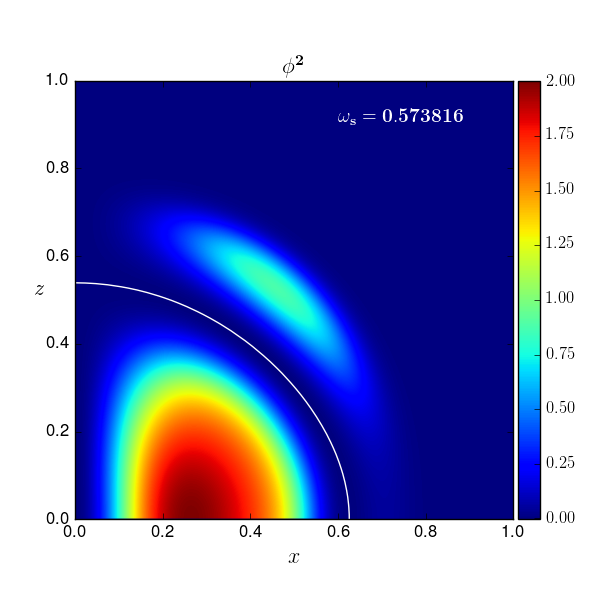
Figure 8: The distribution of the boson field given by the square of its absolute value $\phi^{2}$ on the $xz$-plane, where $z$ is the rotation axis and $x$ is an axis of the equatorial plane, at the turning point ($\phi_{0}=8.78668$) for rotating radially excited solutions (one node, $m=1$, $\kappa=0.05$). The white curve represents the location of the node.

Let us now consider how the boson number (or charge) $Q$ is distributed among the two shells. We therefore define $\phi^{+}$ to be the positive valued field comprehending the first shell, and $\phi^{-}$ the negative valued field comprehending the second shell. Then $Q^{+}=Q(\phi^{+})$ is the charge accumulated in the first shell and $Q^{-}=Q(\phi^{-})$ the charge located in the second one. In Fig. 9 the ratio $Q^{-}/Q^{+}$ is shown. In most solutions the major part of the charge is concentrated in the outer shell, where in some cases it is as high as five times the charge residing in the inner shell. This feature changes in the vicinity of the turning point, where the configurations are characterized by a greater amount of charge in the inner shell. The observed distribution of the charges within the shells might seem surprising at first, when comparing with the field distribution, but the field extends to infinity, and the metric determinant in the volume integral gives more weight to the outer shell.

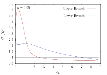
Figure 9: Ratio $Q^{-}/Q^{+}$ of the number of particles residing in the outer ($Q^{-}$) and inner ($Q^{+}$) shell of rotating radially excited solutions (one node, $m=1$, $\kappa=0.05$).

IV.3 Decomposition of the Field

In order to better understand the radial excitations of the scalar field we will now decompose it into a complete set of functions of the coordinates. While the equations are not separable due to nonlinear effects, a decomposition into the set of associated Legendre functions each coupled to a radial function can still be achieved. This decomposition for the boson function $\phi(r,\theta)$ is based on the associated decomposition of the scalar field $\Phi$ itself, whose spatial part would be decomposed into the spherical harmonics $Y_{\ell m}(\theta,\varphi)$ with $m=1$. We therefore write

$$\phi(r,\theta)=\sum_{\ell=|m|}^{\infty}R_{\ell}(r)P^{m}_{\ell}(\theta).$$

Throughout this paper we have dealt only with the particular case of $m=1$. Clearly, the azimuthal quantum number $\ell$, which labels the field’s angular excitations, must then be greater or equal to one. Furthermore, the even parity character of the scalar field results in $R_{\ell}=0$ for all even values of $\ell$. In the implementation of the decomposition the series was truncated at $\ell=11$, giving a very good approximation to the true solution with a maximal relative error of order $10^{-8}$ or better at any point.

Solutions for which the boson frequency $\omega_{s}$ is close to its maximum value possess a scalar field with very small amplitude. The quartic and sextic terms in the potential (II.2) are then negligible across the whole domain. The Klein-Gordon equation eq. (12) then becomes linear. Furthermore, as these solutions approach the trivial one, the spacetime becomes almost flat.

Still it is essential that there is a gravitational potential, since in a flat spacetime, the linear Klein-Gordan equation would not possess localized bound states. In Minskowski spacetime, one would have a complete separation of variables, and one could find solutions for which the bosons would all be in the same state, specified by the quantum numbers $\ell$ and $m$. But these would correspond to free field configurations. The analysis of the localized field configurations of the boson stars, however, shows that the rotating radially excited boson star solutions are all represented by superpositions of states with several quantum numbers $\ell$ (while $m=1$).

In this linear regime, every term in the above decomposition represents a mode with quantum numbers $n,\ell,m$, where $n$ can be seen as to represent the principal quantum number. In this case we recover the relationship $n=1+\ell+s$, where $s$ is the number of associated radial (spherical) nodes.

Fig. 10 shows two solutions in the linear regime for coupling $\kappa=1.0$, and with similar values of the characteristic value of the field at the origin $\phi_{0}$, belonging to different branches. Only the radial functions of the lowest $\ell$ modes are exhibited in the figure. The others have very small amplitudes. The lowest mode in the decomposition with respect to $\ell$ is given by $\ell=1,s=1$, yielding $n=3$ in both cases.

The solution on the upper branch contains more particles in this mode than the solution on the lower branch, and fewer particles in higher $\ell$ modes. For $\ell=7$ and $\ell=11$ the radial functions on the lower and upper branches all contain one radial node. The remaining modes analyzed possess zero radial nodes. Thus, in the linear approximation valid for boson frequencies near the maximum value, the solutions on the lower branch are composed of bosons in more excited (higher $\ell$) modes than those on the upper branch.

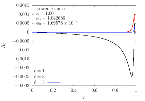
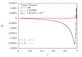
Figure 10: The lowest radial functions $R_{\ell}$ of the decomposition of the scalar field in terms of associated Legendre functions ($m=1$) versus the compactified radial coordinate $\bar{r}$ for rotating radially excited solutions (one node, $\kappa=1.00$) in the linear regime close to the maximum boson frequency.

We now focus on the solutions analyzed in the previous subsection, i.e., we address the solutions of the non-linear regime. In Fig. 11 the radial functions $R_{\ell}$ of the decomposition, whose amplitude is not negligible, are presented. We observe the same qualitative behavior that we saw for the solutions in the linear regime. The larger contribution of the function $R_{3}$ for the solutions on the lower branch translates into the outer shell of the scalar field being closer to the rotational axis.

The above analysis reveals, that the solutions on the upper and lower branches possess a different decomposition into modes. The decomposition for the solution at the turning point is presented in Fig. 12. All modes higher than $\ell=3$ have very small amplitudes in this case. We conclude with the observation that contrary to spherically symmetric boson stars, which are all represented by the lowest spherical harmonic $Y_{00}$, (self interacting) rotating boson stars cannot be formed by bosons in a single mode $Y_{\ell m}$.

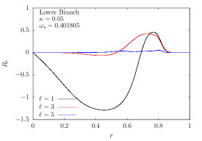
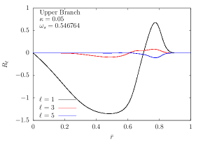
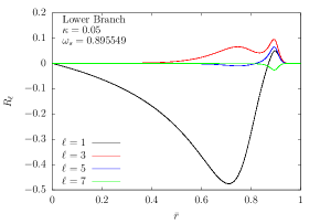
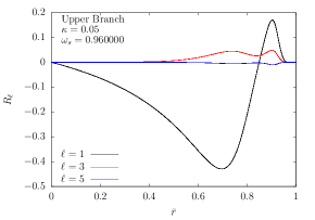
Figure 11: The lowest radial functions $R_{\ell}$ of the decomposition of the scalar field in terms of associated Legendre functions ($m=1$) versus the compactified radial coordinate $\bar{r}$ for rotating radially excited solutions (one node, $\kappa=0.05$). Upper panels: Solutions with similar value of $\phi_{0}$ near the turning point. Lower panels: Solutions with similar value of $\phi_{0}$ for smaller $\phi_{0}$.

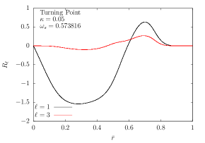
Figure 12: The lowest radial functions $R_{\ell}$ of the decomposition of the scalar field in terms of associated Legendre functions ($m=1$) versus the compactified radial coordinate $\bar{r}$ for the rotating radially excited solution at the turning point (one node, $\kappa=0.05$).

IV.4 Energy Density and Pressures

In order to investigate the energy density and the pressures of the rotating radially excited boson stars, we take a vierbein set $\hat{e}_{a}^{\mu}$, which are eigenvectors of energy momentum tensor. Then $u^{\mu}=\hat{e}_{0}^{\mu}$ is the four velocity of an element of the scalar fluid. The eigenvalues $\lambda_{(a)}$ correspond to the energy density and the pressures as measured by an observer comoving with the fluid, and are found through the relation

$$T_{\mu\nu}\hat{e}^{\mu}_{a}=\lambda_{(a)}\hat{e}_{\nu a},$$ (29)

such that the diagonal energy momentum tensor takes the form $T^{a}_{b}=diag(\lambda_{0},\lambda_{1},\lambda_{2},\lambda_{3})$. The energy density is given by $\rho=-\lambda_{0}$, the radial pressure by $p_{r}=\lambda_{1}$, and the tangential pressure by $p_{\bot}=\lambda_{2}=\lambda_{3}$, since the scalar field constitutes an anisotropic fluid. The diagonal energy momentum tensor is then given by

$$T^{a}_{b} =T_{\mu\nu}\hat{e}^{\mu a}\hat{e}^{\nu}_{b}$$

$$=-\delta^{a}_{b}\left[\frac{1}{2}g^{\rho\tau}\left(\Phi^{\ast}_{,\rho}\Phi_{,\tau}+\Phi^{\ast}_{,\tau}\Phi_{,\rho}\right)+U\left(\lvert\Phi\rvert\right)\right]+\hat{e}^{\mu a}\hat{e}^{\nu}_{b}\left(\Phi^{\ast}_{,\mu}\Phi_{,\nu}+\Phi^{\ast}_{,\nu}\Phi_{,\mu}\right).$$ (30)

The equations of state for the radial and tangential pressure, as derived from the above expression, read

$$p_{r}=\rho-2U,\qquad p_{\bot}=p_{r}-2\partial_{\mu}\phi\partial^{\mu}\phi,$$ (31)

and take the same form as in the spherically symmetric case. At the nodal surface, all of these quantities have the same absolute value, i.e., $\rho=p_{r}=-p_{\bot}$. In contrast to the spherically symmetric boson stars, the tangential pressure is negative at the origin for rotating boson stars. The anisotropy factor $a_{p}$,

$$a_{p}=\frac{p_{r}-p_{\bot}}{p_{r}},$$ (32)

is not well behaved for either nodeless or radially excited rotating boson stars when $p_{r}=0$. It always assumes the value $a_{p}=2$ at the nodal surface (see the equations of state).

The general profile of the energy density and the pressures for the two pairs of solutions analyzed before are shown in Figs. 13, 14 and 15. The energy density and the radial pressure are distributed in a similar manner as the boson field squared. Likewise, both are zero at the origin. The tangential pressure, however, starts with negative values close to the origin and turns positive only in the vicinity of the center of the inner and outer shell, respectively.

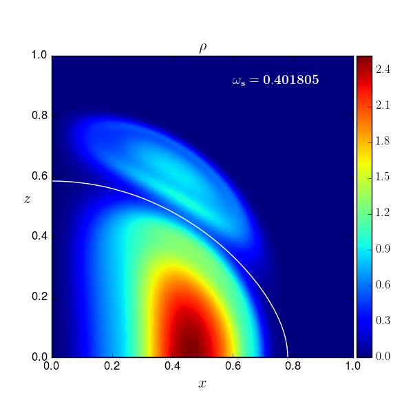
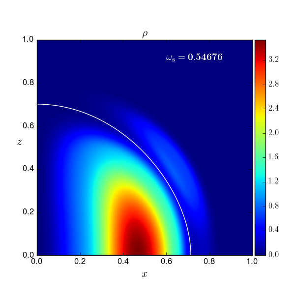
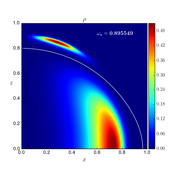
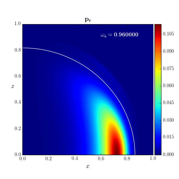
Figure 13: Energy density $\rho$ as measured by an observer at rest with respect to the scalar fluid on the $xz$-plane, where $z$ is the rotation axis and $x$ is an axis of the equatorial plane, for rotating radially excited solutions (one node, $m=1$, $\kappa=0.05$). The white curve represents the location of the node. Upper panels: Solutions with similar values of $\phi_{0}$ near the turning point. Lower panels: Solutions with similar values of $\phi_{0}$ for smaller $\phi_{0}$.

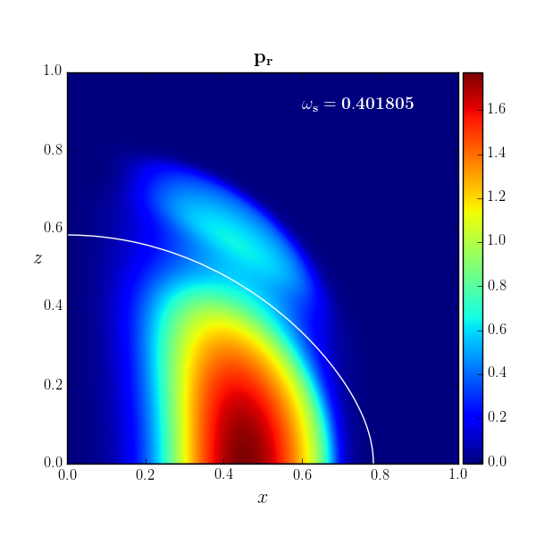
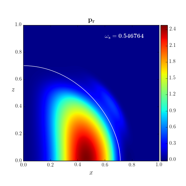
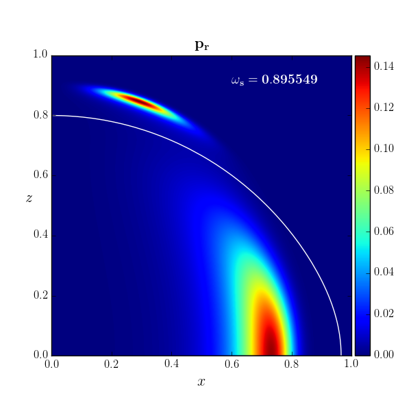
Figure 14: Radial pressure $p_{r}$ as measured by an observer at rest with respect to the scalar fluid on the $xz$-plane, where $z$ is the rotation axis and $x$ is an axis of the equatorial plane, for rotating radially excited solutions (one node, $m=1$, $\kappa=0.05$). The white curve represents the location of the node. Upper panels: Solutions with similar values of $\phi_{0}$ near the turning point. Lower panels: Solutions with similar values of $\phi_{0}$ for smaller $\phi_{0}$.

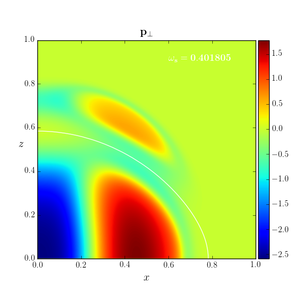
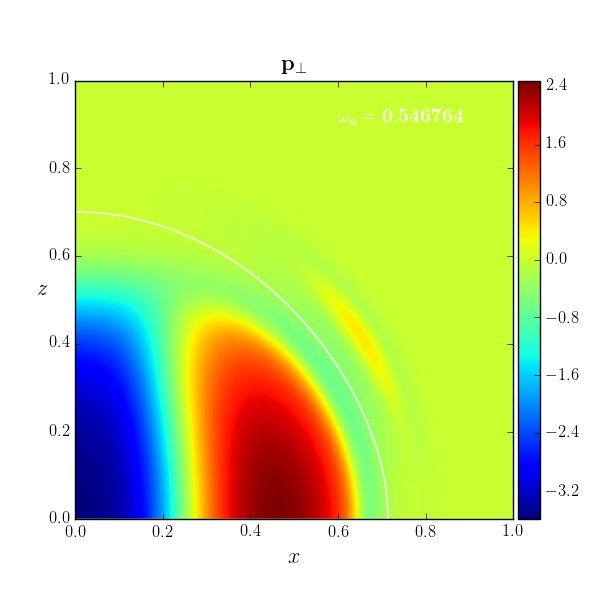
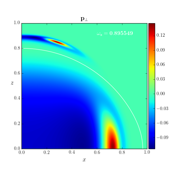
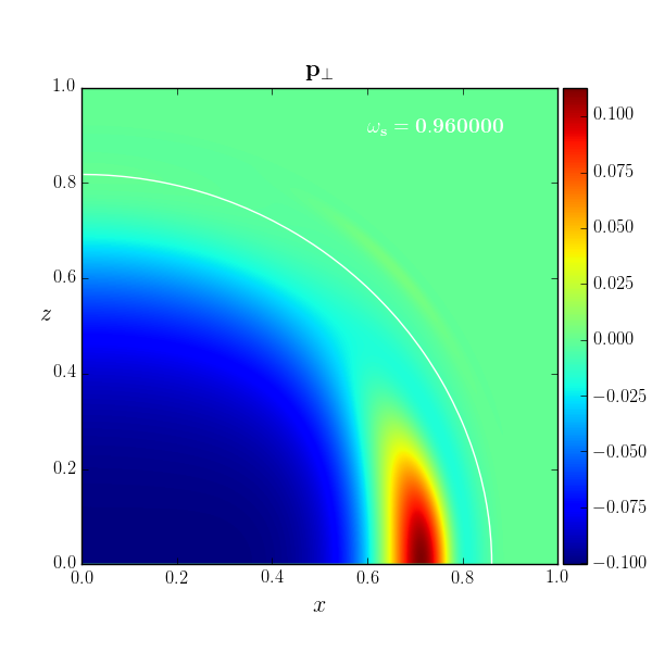
Figure 15: Tangential pressure $p_{\bot}$ as measured by an observer at rest with respect to the scalar fluid on the $xz$-plane, where $z$ is the rotation axis and $x$ is an axis of the equatorial plane, for rotating radially excited solutions (one node, $m=1$, $\kappa=0.05$). The white curve represents the location of the node. Upper panels: Solutions with similar values of $\phi_{0}$ near the turning point. Lower panels: Solutions with similar values of $\phi_{0}$ for smaller $\phi_{0}$.

The turning point solution, whose density and pressures are presented in Fig. 16, is the most compact boson star of the one node set of solutions. The energy density and radial pressure are highly concentrated in the inner shell, while the tangential pressure increases much more rapidly from the origin, assuming modestly negatives values outside the central parts of the shells.

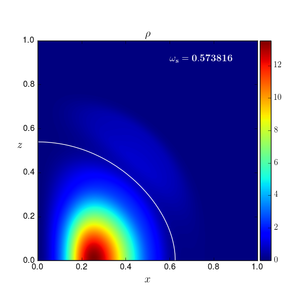
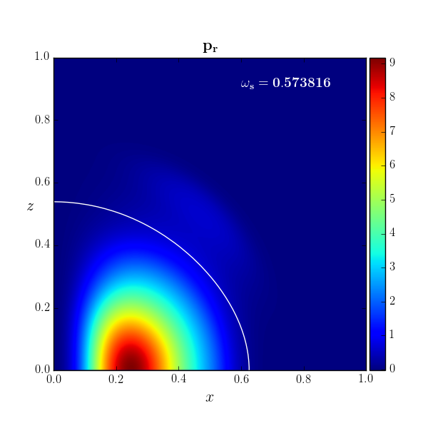
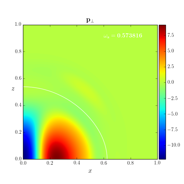
Figure 16: Energy density $\rho$ (upper left panel), radial pressure $p_{r}$ (upper right panel), and tangential pressure $p_{\bot}$ (lower panel) as measured by an observer at rest with respect to the scalar fluid on the $xz$-plane, where $z$ is the rotation axis and $x$ is an axis of the equatorial plane, for the rotating radially excited solution (one node, $m=1$, $\kappa=0.05$) at the turning point. The white curve represents the location of the node.

The equatorial slice for the radial pressure $p_{\bot}$ is shown in more detail in Fig. 17 for the solution at the turning point and a solution close to it located on the upper branch. The figure illustrates that, when both rotation and radial excitation are present, some equilibrium configurations exhibit (albeit very sightly) a negative radial pressure in the equatorial plane, an effect not seen in the nodeless rotating case.

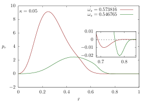
Figure 17: Radial pressure $p_{r}$ as measured by an observer at rest with respect to the scalar fluid in the equatorial plane for the rotating radially excited solution at the turning point and a solution on the upper branch close to it (one node, $m=1$, $\kappa=0.05$). The inset highlights that the radial pressure in the equatorial plane can become slightly negative in the outer region of the outer shell.

IV.5 Stability

We here do not attempt to make a full stability analysis for these sets of solutions. Instead we will analyze the mass $M$ for a given particle number $Q$ together with the binding energy $E_{b}$ of the boson stars, and determine which branch of solutions should more likely be the most stable one, based on energetic grounds. We thus follow similar lines of analysis as performed previously for the spherically symmetric and rotating cases LEE1992251 ; PhysRevD.43.3895 ; PhysRevD.72.064002 ; PhysRevD.77.064025 ; PhysRevD.85.024045 .

Let us start with briefly recalling the stability of the fundamental rotating boson stars in this model PhysRevD.85.024045 . Here arguments from catastrophy theory have indicated, that there should be two stable regions in the full set of nodeless rotating boson stars. When comparing the set of rotating radially excited boson stars with the fundamental one, one realizes, that for every allowed particle number $Q$ of the radially excited solutions, there is a fundamental solution with a lower mass. This suggests that even the most stable radially excited solutions can tunnel to a lower state, and thus will not be absolutely stable. Let us therefore now focus on the relative stability of the radially excited solutions, looking for their most stable subset.

Fig. 18(a) exhibits the mass $M$ versus the particle number $Q$ for the set of rotating radially excited boson stars (with one node) for the coupling constant $\kappa=0.05$. For better identification the lower and upper branch are indicated by distinct colours. Also shown is the straight line $M_{\rm free}=m_{b}Q$, indicating the mass of $Q$ free bosons, and thus representing a boundary line for stability, since solutions with a higher mass for a given particle number $Q$ could decay into $Q$ free particles.

In Fig. 18(a) the upper and lower branch themselves contain a number of subbranches, starting and ending at cusps, where the mass and the particle number assume local or global maxima and minima. From previous mode analyses of spherically symmetric boson stars it is known, that at these cusps the stability of the solutions changes in the sense, that they acquire or lose an unstable mode. Moreover, for a given particle number, the most stable solution should correspond to the one with the lowest mass, while higher mass solutions should be able to tunnel to the lowest mass solution of a given particle number.

Inspection of the data and the figure then suggests that the subset of solutions should be most stable, which starts on the lower branch at the maximal value of $\omega_{s}$ from the vacuum, and reaches the cusp at the global maximum of the mass and the particle number. However, a small subset of this subset of solutions in the vicinity of $Q\approx 500$ forms a swallow tail, as seen in the lower right inset of the figure. Thus in that region for a given value of the particle number there are three (except at the two cusps, where there are two) solutions with different masses.

Since the subset of solutions of the lower branch intersects itself in the $M$-$Q$ diagram, when forming the swallow tail, as marked by the cross in the lower right inset, the subset of most stable solutions would simply jump at the intersection point from the lowest mass branch to the left of the intersection point to the lowest mass branch to the right of the intersection point. All other solution of the swallow tail will have higher masses for a given particle number, and should therefore be more unstable. Note that some of the unstable solutions possess even masses above the mass of the corresponding number of free particles.

According to these considerations, which can be made more stringent by applying arguments from catastrophe theory PhysRevD.43.3895 ; PhysRevD.85.024045 , all the remaining solutions on the lower branch beyond the maximal mass and all solutions on the upper branch should be more unstable than this most stable subset.

However, there is another form of instability endangering the stability of regular rotating compact objects. This is the ergoregion instability, discussed first for boson stars in PhysRevD.77.124044 . We indicate the onset and the termination of the ergoregion for this set of boson stars in the figure by the circles. Clearly, here the ergoregion instability does not arise for the most stable subset of solutions, but it arises only for solutions, where stability has been lost already.

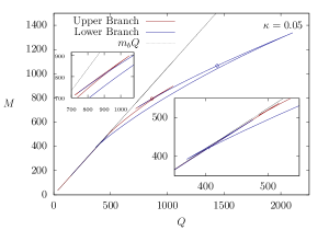
(a)

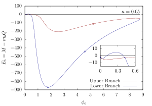
(b)

Figure 18: Left: The mass $M$ of rotating radially excited boson stars ($m=1$) with one node versus the particle number $Q$ ($\kappa=0.05$). The circles indicate the onset and termination of the presence of ergoregions. The mass of $Q$ free particles, $m_{b}Q$ is shown for comparison. Right: The binding energy $E_{b}$ versus the value $\phi_{0}$, characterizing the boson field at the origin, for the same set of solutions. The triangle indicates the maximum mass solution, the crosses indicate an $M$-$Q$ intersection point.

Fig. 18(b) shows the binding energy of this set of solutions along the two branches defined by the value $\phi_{0}$, characterizing the boson field at the origin. Here we note, that except for the small region of the swallow tail around $Q\approx 500$, which is enlarged in the inset and corresponds to small values of $\phi_{0}$, the solutions on the lower branch are always more strongly bound than the solutions on the upper branch.

This further confirms the above assessment, that the most stable solutions reside on two parts of the lower branch. At the global maximal value of the mass (indicated by the triangle in the figure), which corresponds to the global maximal value of the particle number, an unstable mode is expected to arise. While the maximum mass configuration is most strongly bound, it should also contain a zero mode, which should turn into an unstable mode for configurations beyond the maximum mass configuration.

Again, we emphasize, that there is the transition in the swallow tail region around $Q\approx 500$, where part of the lower branch would be more unstable. We indicate by crosses in the inset of the figure the points, where this part of the lower branch intersects itself in the $M$-$Q$ diagram. As noted above, all the solutions between these points, should be more unstable. The most stable set of solutions would directly jump from the first cross to the next cross, since mass, particle number and binding energy are the same for both configurations. Note, that the particle number of the solutions on the lower branch and on the upper branch for a given value of $\phi_{0}$ can differ widely.

V Conclusions

Rotating boson stars are interesting compact objects, formed by a (self-interacting) complex scalar field coupled to gravity. Their angular momentum $J$ is quantized, representing an integer multiple $m$ of their particle number $Q$. Their harmonic time-dependence is governed by the boson frequency $\omega_{s}$, which assumes values in a finite interval, bounded by the boson mass.

Here we have constructed solutions of rotating boson stars with rotational quantum number $m=1$, which are radially excited. The radial excitation is realized by the presence of a nodal surface, where the scalar field vanishes. We have found that the presence of this radial excitation has profound consequences for the set of boson star solutions. They do not form a spiral, when their mass or particle number are considered versus the frequency, as the set of fundamental rotating boson star solutions does. Instead they form a closed loop, starting from the maximal boson frequency at the vacuum solution, reaching a minimal boson frequency and ending again at the maximal boson frequency at the vacuum solution.

By considering the expansion of the scalar field at the origin, one finds the expansion parameter $\phi_{0}$, which can be used to characterize the solutions. In terms of $\phi_{0}$ one finds two branches of solutions, extending between zero and a maximal value of $\phi_{0}$. For each value of $\phi_{0}$ between the two limits there are precisely two boson star solutions. Thus the solutions form two branches of a loop, a lower branch and an upper branch. We have therefore labeled the solutions by their value of $\phi_{0}$ and their location on one of the branches.

The nodal surface of the rotating radially excited boson stars divides the scalar fluid into two shells, an inner shell and an outer shell. The inner shell has the same qualitative properties in both branches and is always centered on the equatorial plane. In contrast, the outer shell’s center can be located at a wide range of values of the polar angle. On the upper branch the outer shell is closer to the equatorial plane, while on the lower one it is nearer to the rotational axis. These radially excited boson stars can thus possess very different distributions of the scalar field.

Boson stars are anisotropic compact objects, possessing different radial and tangential pressures. Here we have also analyzed the energy density and the pressures as seen by a comoving observer for these rotating radially excited boson stars. They all reflect the shell structure seen already for the scalar field itself. Interestingly, the most compact boson star is located at the turning point of the loop, i.e., at the maximal value of $\phi_{0}$.

The scalar field of the boson stars can be decomposed into a set of spherical harmonics with appropriate radial functions. Since the rotating boson stars studied here all possess a rotational quantum number $m=1$ and even parity, the expansion is restricted accordingly. The few lowest odd $\ell$ terms always suffice to obtain an excellent approximation of the solutions. The decomposition of the most compact boson star at the turning point of the loop requires only two terms. While these rotating boson stars always require a superposition of modes, one obtains (at least) two distinct superpositions for each value of the boson frequency inbetween the minimal and maximal values of the frequency.

We have also discussed the stability of the rotating boson stars, following the reasoning of previous work. This has led us to the conclusion that for a given particle number and thus also angular momentum, the solution with the lowest mass and thus the most stable solution, will always belong to the set of fundamental solutions, i.e., be a nodeless solution. Among the solutions with a radial excitation, the most stable solutions reside on the lower branch of solutions below the solution with the maximum mass.

VI Acknowledgments

We would like to acknowledge support by the DFG Research Training Group 1620 Models of Gravity as well as by FP7, Marie Curie Actions, People, International Research Staff Exchange Scheme (IRSES-606096). BK gratefully acknowledges support from Fundamental Research in Natural Sciences by the Ministry of Education and Science of Kazakhstan.

Appendix A Field Equations

The Einstein field equations are solved as a boundary value problem. For simplicity we diagonalize them, so that we work with five coupled elliptic PDEs written in the canonical form

$$r^{2}\partial^{2}_{r}f+\partial^{2}_{\theta}f =-\frac{1}{2}\frac{1}{fl}\Biggl{[}4\kappa r^{2}fl^{2}gU(\phi)-8\kappa m^{2}l^{2}g\omega^{2}\phi^{2}-16\kappa m\omega_{s}rl^{2}g\omega\phi^{2}-8\kappa\omega_{s}^{2}r^{2}l^{2}g\phi^{2}-2\sin^{2}\theta l^{2}\omega^{2}$$

$$+4rfl\partial_{r}f+2\cot\theta fl\partial_{\theta}f+f\partial_{\theta}f\partial_{\theta}l-2l\left(r^{2}\left(\partial_{r}f\right)^{2}+\left(\partial_{\theta}f\right)^{2}\right)+r^{2}f\partial_{r}f\partial_{r}l+4r\sin^{2}\theta l^{2}\omega\partial_{r}\omega$$

$$-2\sin^{2}\theta l^{2}\left(r^{2}\left(\partial_{r}\omega\right)^{2}+\left(\partial_{\theta}\omega\right)^{2}\right)\Biggr{]}.$$ (33)

$$r^{2}\partial^{2}_{r}l+\partial^{2}_{\theta}l =-\frac{1}{2}\frac{1}{fl}\Biggl{[}8\kappa r^{2}l^{3}gU(\phi)+8\kappa\csc^{2}\theta m^{2}fl^{2}g\phi^{2}-8\kappa\frac{l^{3}g}{f}\phi^{2}\left(m^{2}\omega^{2}+2rm\omega_{s}\omega+r^{2}\omega_{s}^{2}\right)+6rfl\partial_{r}l$$

$$+4\cot^{2}\theta fl\partial_{\theta}l-f\left(r^{2}\left(\partial_{r}l\right)^{2}+\left(\partial_{\theta}l\right)^{2}\right)\Biggr{]}.$$ (34)

$$r^{2}\partial^{2}_{r}g+\partial^{2}_{\theta}g =-\frac{1}{2}\frac{1}{fl}\Biggl{[}8\kappa m^{2}\csc^{2}\theta flg^{2}\phi^{2}-2\sin^{2}\theta\frac{l^{2}g}{f}\omega^{2}+8\kappa flg\left(\partial_{\theta}\phi\right)^{2}+4rfl\partial_{r}g-2\cot\theta fl\partial_{\theta}g$$

$$-2\frac{fl}{g}\left(r^{2}\left(\partial_{r}g\right)^{2}+\left(\partial_{\theta}g\right)^{2}\right)+f\left(r^{2}\partial_{r}l\partial_{r}g-\partial_{\theta}l\partial_{\theta}g\right)+2\frac{lg}{f}\left(\partial_{\theta}f\right)^{2}-2\cot\theta fg\partial_{\theta}l-3\frac{fg}{l}\left(\partial_{\theta}l\right)^{2}$$

$$+2fg\partial_{\theta}^{2}l+4r\sin^{2}\theta\frac{l^{2}g}{f}\omega\partial_{r}\omega-2\sin^{2}\theta\frac{l^{2}g}{f}\left(r^{2}\left(\partial_{r}\omega\right)^{2}+2\left(\partial_{\theta}\omega\right)^{2}\right)\Biggr{]}.$$ (35)

$$r^{2}\partial^{2}_{r}\omega+\partial^{2}_{\theta}\omega =-\frac{1}{2}\frac{1}{fl}\Biggl{[}8\kappa\csc^{2}\theta m^{2}flg\omega\phi^{2}-8\kappa r\csc^{2}\theta m\omega_{s}flg\phi^{2}-4fl\omega+4rfl\partial_{r}\omega+6\cot\theta fl\partial_{\theta}\omega$$

$$-4l\left(r^{2}\partial_{r}f\partial_{r}\omega+\partial_{\theta}f\partial_{\theta}\omega\right)+3f\left(r^{2}\partial_{r}l\partial_{r}\omega+\partial_{\theta}l\partial_{\theta}\omega\right)+4rl\omega\partial_{r}f-3rf\omega\partial_{r}l\Biggr{]}.$$ (36)

$$r^{2}\partial^{2}_{r}\phi+\partial^{2}_{\theta}\phi =-\frac{1}{2}\frac{1}{fl}\Biggl{[}-r^{2}l^{2}g\frac{\partial U\left(\phi\right)}{\partial\phi}-2\csc^{2}\theta m^{2}flg\phi+2\frac{l^{2}g}{f}\left(\omega m+r\omega_{s}\right)^{2}\phi+4rfl\partial_{r}\phi+2\cot\theta fl\partial_{\theta}\phi$$

$$+f\left(r^{2}\partial_{r}l\partial_{r}\phi+\partial_{\theta}l\partial_{\theta}\phi\right)\Biggr{]}.$$ (37)

Appendix B Energy Density and Vierbein Components

The energy density as measured by a particle comoving with the scalar fluid, given by $-T^{0}_{0}$ in eq. (IV.4) reads

$$\rho=\frac{\phi^{2}\omega_{s}^{2}}{f}+\frac{f}{glr^{2}}\left[r^{2}\left(\partial_{r}\phi\right)^{2}+\left(\partial_{\theta}\phi\right)^{2}\right]+\frac{2\phi^{2}\omega_{s}m\omega}{fr}+\frac{\phi^{2}m^{2}}{lr^{2}\sin^{2}\theta}\left(\frac{l}{f}\omega^{2}\sin^{2}\theta-f\right)+U.$$ (38)

The eigenvector associated with the energy density is simply the four velocity of the fluid, $u^{\mu}=u^{t}(1,0,0,\Omega)$, such that $\Omega=u^{\varphi}/u^{t}=d\varphi/dt$ is its angular velocity. In extended form it reads

$$\hat{e}^{\mu}_{0}=\left(\begin{array}[]{c}\displaystyle\frac{\sqrt{l}\sin\theta(m\omega+\omega_{s}r)}{\sqrt{-f(-lm^{2}\omega^{2}\sin^{2}\theta-2m\omega_{s}l\omega r\sin^{2}\theta-\omega_{s}^{2}lr^{2}\sin^{2}\theta+m^{2}f^{2})}}\\[5.0pt] 0\\[5.0pt] 0\\[5.0pt] \displaystyle\frac{ml\omega^{2}\sin^{2}\theta+\omega_{s}l\omega r\sin^{2}\theta-mf^{2}}{\sqrt{-fl(-lm^{2}\omega^{2}\sin^{2}\theta-2m\omega_{s}l\omega r\sin^{2}\theta-\omega_{s}^{2}lr^{2}\sin^{2}\theta+m^{2}f^{2})}r\sin\theta}\end{array}\right).$$ (39)

The eigenvector associated with the radial pressure reads

$$\hat{e}^{\mu}_{1}=\left(\begin{array}[]{c}0\\[5.0pt] \displaystyle\frac{\sqrt{flg\left[r^{2}\left(\partial_{r}\phi\right)^{2}+\left(\partial_{\theta}\phi\right)^{2}\right]}r\partial_{r}\phi}{lg\left[r^{2}\left(\partial_{r}\phi\right)^{2}+\left(\partial_{\theta}\phi\right)^{2}\right]}\\[20.0pt] \displaystyle\frac{\sqrt{flg\left[r^{2}\left(\partial_{r}\phi\right)^{2}+\left(\partial_{\theta}\phi\right)^{2}\right]}\partial_{\theta}\phi}{lgr\left[r^{2}\left(\partial_{r}\phi\right)^{2}+\left(\partial_{\theta}\phi\right)^{2}\right]}\\[5.0pt] 0\end{array}\right).$$

The two eigenvectors associated with the tangential pressure are given by

$$\hat{e}^{\mu}_{2}=\left(\begin{array}[]{c}0\\[5.0pt] \displaystyle-\frac{\sqrt{flg\left[r^{2}\left(\partial_{r}\phi\right)^{2}+\left(\partial_{\theta}\phi\right)^{2}\right]}\partial_{\theta}\phi}{lg\left[r^{2}\left(\partial_{r}\phi\right)^{2}+\left(\partial_{\theta}\phi\right)^{2}\right]}\\[20.0pt] \displaystyle\frac{\sqrt{flg\left[r^{2}\left(\partial_{r}\phi\right)^{2}+\left(\partial_{\theta}\phi\right)^{2}\right]}\partial_{r}\phi}{lg\left[r^{2}\left(\partial_{r}\phi\right)^{2}+\left(\partial_{\theta}\phi\right)^{2}\right]}\\[5.0pt] 0\end{array}\right),$$

$$\hat{e}^{\mu}_{3}=\left(\begin{array}[]{c}\displaystyle\frac{-m\sqrt{f}}{\sqrt{(l\omega^{2}\sin^{2}\theta-f^{2})m^{2}+2lm\omega\omega_{s}r\sin^{2}\theta+l\omega_{s}^{2}r^{2}\sin^{2}\theta}}\\[5.0pt] 0\\[5.0pt] 0\\[5.0pt] \displaystyle\frac{\omega_{s}\sqrt{f}}{\sqrt{(l\omega^{2}\sin^{2}\theta-f^{2})m^{2}+2lm\omega\omega_{s}r\sin^{2}\theta+l\omega_{s}^{2}r^{2}\sin^{2}\theta}}\\ \end{array}\right).$$

References

- (1) D. A. Feinblum and W. A. McKinley, “Stable states of a scalar particle in its own gravational field,” Phys. Rev., vol. 168, pp. 1445–1450, Apr 1968.
- (2) D. J. Kaup, “Klein-gordon geon,” Phys. Rev., vol. 172, pp. 1331–1342, Aug 1968.
- (3) R. Ruffini and S. Bonazzola, “Systems of self-gravitating particles in general relativity and the concept of an equation of state,” Phys. Rev., vol. 187, pp. 1767–1783, Nov 1969.
- (4) P. Jetzer, “Boson stars,” Physics Reports, vol. 220, no. 4, pp. 163 – 227, 1992.
- (5) T. Lee and Y. Pang, “Nontopological solitons,” Physics Reports, vol. 221, no. 5, pp. 251 – 350, 1992.
- (6) A. R. Liddle and M. S. Madsen, “The structure and formation of boson stars,” International Journal of Modern Physics D, vol. 01, no. 01, pp. 101–143, 1992.
- (7) S. L. Liebling and C. Palenzuela, “Dynamical boson stars,” Living Reviews in Relativity, vol. 15, p. 6, May 2012.
- (8) E. W. Mielke and F. E. Schunck, “Boson stars: Early history and recent prospects,” 8th Marcel Grossmann Meeting (MG 8), p. 1607, Jun 1997.
- (9) F. E. Schunck and E. W. Mielke, “General relativistic boson stars,” Classical and Quantum Gravity, vol. 20, no. 20, p. R301, 2003.
- (10) M. Colpi, S. L. Shapiro, and I. Wasserman, “Boson stars: Gravitational equilibria of self-interacting scalar fields,” Phys. Rev. Lett., vol. 57, pp. 2485–2488, Nov 1986.
- (11) R. Friedberg, T. D. Lee, and Y. Pang, “Scalar soliton stars and black holes,” Phys. Rev. D, vol. 35, pp. 3658–3677, Jun 1987.
- (12) F. S. Guzmán and J. M. Rueda-Becerril, “Spherical boson stars as black hole mimickers,” Phys. Rev. D, vol. 80, p. 084023, Oct 2009.
- (13) D. F. Torres, S. Capozziello, and G. Lambiase, “Supermassive boson star at the galactic center?,” Phys. Rev. D, vol. 62, p. 104012, Oct 2000.
- (14) E. W. Mielke and F. E. Schunck, “Nontopological scalar soliton as dark matter halo,” Phys. Rev. D, vol. 66, p. 023503, Jun 2002.
- (15) F. E. Schunck, B. Fuchs, and E. W. Mielke, “Scalar field haloes as gravitational lenses,” Monthly Notices of the Royal Astronomical Society, vol. 369, no. 1, pp. 485–491, 2006.
- (16) A. Bernal, J. Barranco, D. Alic, and C. Palenzuela, “Multistate boson stars,” Phys. Rev. D, vol. 81, p. 044031, Feb 2010.
- (17) L. A. Ureña López and A. Bernal, “Bosonic gas as a galactic dark matter halo,” Phys. Rev. D, vol. 82, p. 123535, Dec 2010.
- (18) F. E. Schunck and E. W. Mielke, “Rotating boson star as an effective mass torus in general relativity,” Physics Letters A, vol. 249, no. 5, pp. 389 – 394, 1998.
- (19) B. Kleihaus, J. Kunz, and M. List, “Rotating boson stars and -balls,” Phys. Rev. D, vol. 72, p. 064002, Sep 2005.
- (20) B. Kleihaus, J. Kunz, M. List, and I. Schaffer, “Rotating boson stars and -balls. ii. negative parity and ergoregions,” Phys. Rev. D, vol. 77, p. 064025, Mar 2008.
- (21) B. Kleihaus, J. Kunz, and S. Schneider, “Stable phases of boson stars,” Phys. Rev. D, vol. 85, p. 024045, Jan 2012.
- (22) E. W. Mielke and F. E. Schunck, “Boson stars: alternatives to primordial black holes?,” Nuclear Physics B, vol. 564, no. 1, pp. 185 – 203, 2000.
- (23) F. D. Ryan, “Spinning boson stars with large self-interaction,” Phys. Rev. D, vol. 55, pp. 6081–6091, May 1997.
- (24) F. E. Schunck and E. W. Mielke, “Boson stars: Rotation, formation, and evolution,” General Relativity and Gravitation, vol. 31, pp. 787–798, May 1999.
- (25) S. Yoshida and Y. Eriguchi, “Rotating boson stars in general relativity,” Phys. Rev. D, vol. 56, pp. 762–771, Jul 1997.
- (26) V. Cardoso, P. Pani, M. Cadoni, and M. Cavaglià, “Ergoregion instability of ultracompact astrophysical objects,” Phys. Rev. D, vol. 77, p. 124044, Jun 2008.
- (27) F. E. Schunck and E. W. Mielke, Rotating Boson Stars, pp. 138–151. Berlin, Heidelberg: Springer Berlin Heidelberg, 1996.
- (28) W. Deppert and E. W. Mielke, “Localized solutions of the nonlinear heisenberg-klein-gordon equation: In flat and exterior schwarzschild space-time,” Phys. Rev. D, vol. 20, pp. 1303–1312, Sep 1979.
- (29) E. W. Mielke and R. Scherzer, “Geon-type solutions of the nonlinear heisenberg-klein-gordon equation,” Phys. Rev. D, vol. 24, pp. 2111–2126, Oct 1981.
- (30) R. Friedberg, T. D. Lee, and Y. Pang, “Scalar Soliton Stars and Black Holes,” Phys. Rev., vol. D35, p. 3658, 1987. [,73(1986)].
- (31) F. V. Kusmartsev, E. W. Mielke, and F. E. Schunck, “Gravitational stability of boson stars,” Phys. Rev. D, vol. 43, pp. 3895–3901, Jun 1991.
- (32) M. S. Volkov and E. Wöhnert, “Spinning q-balls,” Phys. Rev. D, vol. 66, p. 085003, Oct 2002.
- (33) B. Kleihaus and J. Kunz, “Rotating hairy black holes,” Phys. Rev. Lett., vol. 86, pp. 3704–3707, Apr 2001.
- (34) W. Schönauer and R. Weiß, “Efficient vectorizable PDE solvers,” J. Comput. Appl. Math., vol. 27, p. 279, 1989.