Framization of a Temperley-Lieb algebra of type $\mathtt{B}$

Abstract.

We extend the Framization of the Temperley-Lieb algebra to Coxeter systems of type $\mathtt{B}$. We first define a natural extension of the classical Temperley-Lieb algebra to Coxeter systems of type $\mathtt{B}$ and prove that such an extension supports a unique linear Markov trace function. We then introduce the Framization of the Temperley-Lieb algebra of type $\mathtt{B}$ as a quotient of the Yokonuma-Hecke algebra of type $\mathtt{B}$. The main theorem provides necessary and sufficient conditions for the Markov trace defined on the Yokonuma-Hecke algebra of type $\mathtt{B}$ to pass to the quotient algebra. Using the main theorem, we construct invariants for framed links and classical links inside the solid torus.

1. Introduction

The Temperley-Lieb algebra appeared originally in the study of the Potts model in statistical mechanics and in the ice-type model in two dimensions [30]. In the 1980’s the Temperley-Lieb algebra was rediscovered by Jones in the context of von Neumann algebras [18] and later as a quotient of the Hecke algebra [19]. The Hecke algebra supports a unique inductive linear trace that can be rescaled according to the Markov equivalence for braids and under certain conditions it passes to the Temperley-Lieb algebra. This procedure leads to the definition of the Jones polynomial. For these reasons, the Hecke algebra and the Temperley-Lieb algebra are often considered as knot algebras. Another notable example of a knot algebra is the BMW algebra [1, 29].

Framization is a technique introduced by Juyumaya and Lambropoulou that produces new knot algebras associated to framed knots and links [26]. Framization adds new generators, called the framing generators, to the generating set of a known knot algebra and defines relations between the original and the framing generators of the algebra. From an algebraic point of view, a knot algebra might have multiple candidates that are valid. However, since the motivation of the technique is to obtain new polynomial invariants for (framed) links, candidates that produce new, non-trivial link invariants are preferred. In particular, when multiple framization candidates for a knot algebra are considered, the framization of the algebra that is most natural from a topological point of view is chosen [14].

A basic example of framization is the Yokonuma-Hecke algebra of type $\mathtt{A}$, denoted ${\rm Y}_{d,n}(u)$. It was introduced in the context of Chevalley groups in [32] and can be regarded as the framization of the Hecke algebra. Juyumaya fine-tuned the presentation of ${\rm Y}_{d,n}(u)$ by giving a natural description in terms of the framed braid group [20]. In recent years, framizations of several knot algebras have appeared [22, 26, 23, 25, 13] that led to Jones-type invariants for framed [26], classical [26, 5], and singular links [24].

The Framization of the Temperley-Lieb algebra ${\rm FTL}_{d,n}(q)$ was introduced in [14] as a quotient of ${\rm Y}_{d,n}(u)$. From this, a family of one-variable invariants for classical links in $S^{3}$, denoted $\theta_{d}(q)$, was derived by finding the necessary and sufficient conditions for the trace of ${\rm Y}_{d,n}(u)$ to pass to the quotient algebra. For $d=1$, the invariant $\theta_{1}$ coincides with the Jones polynomial while for $d\neq 1$, $\theta_{d}$ is not topologically equivalent to the Jones polynomial on links [14]. More recently, Goundaroulis and Lambropoulou generalized the invariants $\theta_{d}(q)$ to a new two-variable invariant that is stronger than the Jones polynomial on links and that can also detect the Thistlethwaite link [15].

All the results that are mentioned above are related to the Coxeter group of type $\mathtt{A}$. However, there is a growing interest in framizations of algebras that are related to Coxeter systems of type $\mathtt{B}$. Indeed, the affine and cyclotomic Yokonuma-Hecke algebras were introduced in [4], while in [10] Flores and collaborators introduced ${\rm Y}_{d,n}^{\mathtt{B}}(\mathsf{u},\mathsf{v})$, the Yokonuma-Hecke algebra of type $\mathtt{B}$.

In this paper we extend the Framization of the Temperley-Lieb algebra of type $\mathtt{A}$ to Coxeter groups of type $\mathtt{B}$ by implementing the methods of [10]. We first consider the generalized Temperley-Lieb algebra that is associated to an arbitrary Coxeter system [16], and specialize it to the case of Coxeter systems of type $\mathtt{B}$. We denote this algebra by ${\rm TL}_{n}^{\mathtt{B}}(\mathsf{u},\mathsf{v})$ and show that it emerges naturally as a quotient of the Hecke algebra of type $\mathtt{B}$, denoted ${\rm H}_{n}(\mathsf{u},\mathsf{v})$. We then compute the necessary and sufficient conditions for the Markov trace of ${\rm H}_{n}(\mathsf{u},\mathsf{v})$ [27] to pass to the quotient algebra. The Framization of the Temperley-Lieb algebra of type $\mathtt{B}$, which is denoted ${\rm FTL}_{d,n}^{\mathtt{B}}(\mathsf{u},\mathsf{v})$, is defined as a quotient of the algebra ${\rm Y}_{d,n}^{\mathtt{B}}(\mathsf{u},\mathsf{v})$. For $d=1$, the algebra ${\rm FTL}_{d,n}^{\mathtt{B}}(\mathsf{u},\mathsf{v})$ coincides with ${\rm TL}_{n}^{\mathtt{B}}(\mathsf{u},\mathsf{v})$. The main theorem determines the necessary and sufficient conditions such that the trace of ${\rm Y}_{d,n}^{\mathtt{B}}(\mathsf{u},\mathsf{v})$ [10] passes to ${\rm FTL}_{d,n}^{\mathtt{B}}(\mathsf{u},\mathsf{v})$. Finally, we investigate the conditions of the main theorem which generate topologically non-trivial invariants for framed and classical links and we define those invariants.

The outline of the paper is as follows. In Section 2 we introduce the notation and we present the classical braid group, the framed braid group, the algebra ${\rm H}_{n}(\mathsf{u},\mathsf{v})$, its framization ${\rm Y}_{d,n}^{\mathtt{B}}(\mathsf{u},\mathsf{v})$, and the Framization of the Temperley-Lieb algebra of type $\mathtt{A}$. In Section 3 we introduce the Temperley-Lieb algebra associated to the Coxeter group of type ${\mathtt{B}}$, denoted ${\rm TL}_{n}^{\mathtt{B}}(\mathsf{u},\mathsf{v})$. We also determine the necessary and sufficient conditions such that the trace on ${\rm H}_{n}(\mathsf{u},\mathsf{v})$ passes to the algebra ${\rm TL}_{n}^{\mathtt{B}}(\mathsf{u},\mathsf{v})$ and construct the corresponding link invariants. In Section 4 we present the algebra ${\rm FTL}_{d,n}^{\mathtt{B}}(\mathsf{u},\mathsf{v})$ as a quotient of the algebra ${\rm Y}_{d,n}^{\mathtt{B}}(\mathsf{u},\mathsf{v})$ modulo an appropriate two-sided ideal and determine the necessary and sufficient conditions so that the Markov trace defined on the algebra ${\rm Y}_{d,n}^{\mathtt{B}}(\mathsf{u},\mathsf{v})$ passes to the quotient algebra. In Section 5 we use the trace on ${\rm FTL}_{d,n}^{\mathtt{B}}(\mathsf{u},\mathsf{v})$ to define invariants for framed and classical links and provide a set of skein relations for both cases. Finally, we show that the invariants for classical links from ${\rm FTL}_{d,n}^{\mathtt{B}}(\mathsf{u},\mathsf{v})$ are stronger than the Jones polynomial in the solid torus since they distinguish more pairs of affine links.

2. Preliminaries

Let $\mathsf{u}$, $\mathsf{v}$ be indeterminates. With the term algebra we mean an associative algebra with unity over $\mathbb{K}:=\mathbb{C}(\mathsf{u},\mathsf{v})$.

2.1. Groups of type ${\mathtt{B}}_{n}$

For $n\geq 2$, we define the Coxeter group of type ${\mathtt{B}}_{n}$, denoted by $W_{n}$, as the finite Coxeter group associated to the following Dynkin diagram:

Let $\mathtt{r}_{k}=\mathtt{s}_{k-1}\ldots\mathtt{s}_{1}\mathtt{r}_{1}\mathtt{s}_{1}\ldots\mathtt{s}_{k-1}$ for $2\leq k\leq n$. Every element $w\in W_{n}$ can be written uniquely in a reduced expression as follows [11]: $w=w_{1}\ldots w_{n}$ with $w_{k}\in\mathtt{N}_{k}$, $1\leq k\leq n$, where

(2.1) $$\mathtt{N}_{k}:=\left\{1,\mathtt{r}_{k},\mathtt{s}_{k-1}\cdots\mathtt{s}_{i},\mathtt{s}_{k-1}\cdots\mathtt{s}_{i}\mathtt{r}_{i}\,;\,1\leq i\leq k-1\right\}.$$

The braid group of type ${\mathtt{B}}_{n}$ associated to $W_{n}$, is defined as the group $\widetilde{W}_{n}$ generated by $\rho_{1},\sigma_{1},\ldots,\sigma_{n-1}$ subject to the following relations

(2.2) $$\begin{array}[]{rcll}\sigma_{i}\sigma_{j}&=&\sigma_{j}\sigma_{i}&\text{ for}\quad|i-j|>1,\\ \sigma_{i}\sigma_{j}\sigma_{i}&=&\sigma_{j}\sigma_{i}\sigma_{j}&\text{ for}\quad|i-j|=1,\\ \rho_{1}\sigma_{i}&=&\sigma_{i}\rho_{1}&\text{ for}\quad i>1,\\ \rho_{1}\sigma_{1}\rho_{1}\sigma_{1}&=&\sigma_{1}\rho_{1}\sigma_{1}\rho_{1}.&\end{array}$$

Geometrically, braids of type ${\mathtt{B}}_{n}$ can be viewed as classical braids of type ${\mathtt{A}}_{n+1}$ with $n+1$ strands, where the first strand is identically fixed and is called ‘the fixed strand’. The 2nd, …, $(n+1)$st strands are renamed from 1 to $n$ and they are called ‘the moving strands’. The ‘loop’ generator $\rho_{1}$ corresponds to the looping of the first moving strand around the fixed strand in the right-handed sense (see Fig. 2).

The $d$-modular framed braid group of type $\mathtt{B}_{n}$ is defined as follows:

$$\mathcal{F}^{\mathtt{B}}_{d,n}:=\left(C_{d}\right)^{n}\rtimes\widetilde{W}_{n},$$

where $C_{d}:=\langle t\ |\ t^{d}=1\rangle$, is the cyclic group of order $d$, and the action of $\widetilde{W}_{n}$ on $C_{d}$ is given by: $t_{j}\sigma_{i}=\sigma_{i}t_{\mathtt{s}_{i}(j)}$ and $t_{i}\rho_{1}=\rho_{1}t_{i}$, for $1\leq i\leq n$. In both cases $t_{i}$ is the element of $(C_{d})^{n}$ that has $t$ in the $i^{th}$ position and $1$ everywhere else. For $1\leq i,j\leq n$ and $m\in\{0,\ldots,d-1\}$, we define the following elements on $\mathbb{C}\mathcal{F}^{\mathtt{B}}_{d,n}$:

(2.3) $$e_{i,j}^{(m)}=\frac{1}{d}\sum_{s=0}^{d-1}t_{i}^{m+s}t_{j}^{-s}\quad\mbox{and}\quad f_{i}=\frac{1}{d}\sum_{k=0}^{d-1}t_{i}^{k}.$$

For $j=i+1$, we denote $e_{i}^{(m)}:=e_{i,i+1}^{(m)}$ and $e_{i,j}:=e_{i,j}^{(0)}$. Note that $e_{i,j}^{(m)}$ and $f_{i}$ are idempotent elements.

2.2. The Hecke algebra of type ${\mathtt{B}}$

The Hecke algebra of type $\mathtt{B}$, denoted by ${\rm H}_{n}(\mathsf{u},\mathsf{v})$, can be considered as the quotient of $\mathbb{K}[{\widetilde{W}}_{n}]$ modulo the two-sided ideal that is generated by the following elements:

$$\sigma_{i}^{2}-(\mathsf{u}-\mathsf{u}^{-1})\sigma_{i}-1\quad\mbox{and}\quad\rho_{1}^{2}-(\mathsf{v}-\mathsf{v}^{-1})\rho_{1}-1.$$

In terms of generators and relations, ${\rm H}_{n}(\mathsf{u},\mathsf{v})$ is the algebra that is generated by the elements $b_{1},g_{1},\ldots,g_{n-1}$ which are subject to the following relations:

$$\begin{array}[]{cccl}g_{i}g_{j}&=&g_{j}g_{i}&\text{for all}\quad|i-j|>1,\\ g_{i}g_{i+1}g_{i}&=&g_{i+1}g_{i}g_{i+1}&\text{for all}\quad i=1,\ldots,n-2,\\ g_{1}b_{1}g_{1}b_{1}&=&b_{1}g_{1}b_{1}g_{1},&\\ g_{i}^{2}&=&1+(\mathsf{u}-\mathsf{u}^{-1})g_{i}&\text{for all}\quad i,\\ b_{1}^{2}&=&1+(\mathsf{v}-\mathsf{v}^{-1})b_{1}.&\end{array}$$

The dimension of ${\rm H}_{n}(\mathsf{u},\mathsf{v})$ is $2^{n}n!$ and for $\mathsf{u}=\mathsf{v}=1$ it coincides with $\mathbb{K}[W_{n}]$. Consider now the following subsets of ${\rm H}_{n}(\mathsf{u},\mathsf{v})$:

$$\mathtt{M}_{1}=\{1,\,b_{1}\},\quad\mathtt{M}_{2}=\{1,\,b_{2},\,g_{1},\,g_{1}b_{1}\},\ \ldots,\ \mathtt{M}_{n}=\{1,\,b_{n},\,\,g_{n-1}x\ |\ x\in\mathtt{M}_{n-1}\}.$$

where $b_{k}:=g_{k-1}\dots g_{1}b_{1}g_{1}^{-1}\dots g_{k-1}^{-1}$, for all $2\leq k\leq n$. The following set is a linear basis for the algebra ${\rm H}_{n}(\mathsf{u},\mathsf{v})$:

(2.4) $${\mathtt{C}}_{n}=\left\{m_{1}m_{2}\ldots m_{n}\ |\ m_{i}\in\mathtt{M}_{i}\right\}.$$

There exists a natural epimorphism $\widetilde{W}_{n}\rightarrow{\rm H}_{n}(\mathsf{u},\mathsf{v})$ sending $\sigma_{i}\mapsto g_{i}$ and $\rho_{1}\mapsto b_{1}$. Additionally, the Hecke algebra of type ${\mathtt{B}}$ supports a unique Markov trace function [11]. Indeed, for any indeterminate $z,y$ there exists a linear trace:

$${\rm\tau}:\cup_{n=1}^{\infty}{\rm H}_{n}(\mathsf{u},\mathsf{v})\rightarrow\mathbb{K}[z,y]$$

that is defined inductively by the following four rules:

$$\begin{array}[]{lllll}(1)&{\rm\tau}(\mathbf{1}_{n+1})&=1,&\mbox{for all }n&\\ (2)&{\rm\tau}(ab)&={\rm\tau}(ba),&a,b\in{\rm H}_{n}(q)&(\mbox{Conjugation property})\\ (3)&{\rm\tau}(ag_{n})&=z\,{\rm\tau}(a),&a\in{\rm H}_{n}(q)&(\mbox{Markov property for braiding generators})\\ (4)&{\rm\tau}(ab_{n+1})&=y\,{\rm\tau}(a),&a\in{\rm H}_{n}(q)&(\mbox{Markov property for looping generator}),\end{array}$$

Remark 1.

A different presentation is often used for the algebra ${\rm H}_{n}(\mathsf{u},\mathsf{v})$ that involves parameters $q$ and $Q$, as well as different quadratic relations. More precisely, the quadratic relations are the following:

$$(\overline{g}_{i})^{2}=(q-1)\overline{g}_{i}+q\quad\mbox{and}\quad(\overline{b}_{1})^{2}=(Q-1)\overline{b}_{1}+Q.$$

One can switch between the two presentations by taking $\overline{g}_{i}=\mathsf{u}g_{i}$, $\overline{b}_{1}=\mathsf{v}b_{1}$, $q=\mathsf{u}^{2}$ and $Q=\mathsf{v}^{2}$.

By introducing the term $\lambda=\frac{z-(\mathsf{u}-\mathsf{u}^{-1})}{z}$, one can re-scale $\tau$ so that it satisfies the braid equivalence in the solid torus [27, Theorem 3]. By normalizing $\tau$, link invariants in the solid torus can be defined. Indeed, we have [27, Definition 1]:

(2.5) $$P^{\mathtt{B}}(\mathsf{u},\mathsf{v},z,y)(\widehat{\alpha})=\left(\frac{1-\lambda}{\sqrt{\lambda}(\mathsf{u}-\mathsf{u}^{-1})}\right)^{n-1}\left(\sqrt{\lambda}\right)^{\varepsilon(\alpha)}\tau\left(\pi(\alpha)\right),$$

where $\widehat{\alpha}$ is the closure of the braid $\alpha$ inside the solid torus, $\pi$ is the natural epimorphism $\widetilde{W}_{n}\rightarrow{\rm H}_{n}(\mathsf{u},\mathsf{v})$, and $\varepsilon(\alpha)$ is the algebraic sum of the exponents of the braiding generators in $\alpha$. Furthermore, the invariant $P^{\mathtt{B}}$ can be defined completely by the following two skein relations:

(2.6) $$\frac{1}{\sqrt{\lambda}}\ P^{\mathtt{B}}(L_{+})-\sqrt{\lambda}\ P^{\mathtt{B}}(L_{-}) =\left(\mathsf{u}-\mathsf{u}^{-1}\right)P^{\mathtt{B}}(L_{0})$$

(2.7) $$P^{\mathtt{B}}(M_{+})-P^{\mathtt{B}}(M_{-}) =\left(\mathsf{v}-\mathsf{v}^{-1}\right)P^{\mathtt{B}}(M_{0}),$$

where $L_{+}$, $L_{-}$, $L_{0}$, $M_{+}$ , $M_{-}$ and $M_{0}$ are as shown in Fig. 1.

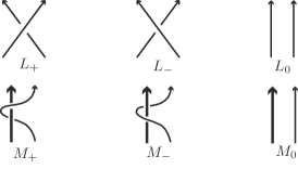
Figure 1. The elements $L_{+}$, $L_{-}$, $L_{0}$ constitute a Conway triple. The elements $M_{+}$ , $M_{-}$ and $M_{0}$ involve the fixed strand (shown in bold).

2.3. The framization of the Hecke algebra of type ${\mathtt{B}}$.

The framization of the Hecke algebra of type $\mathtt{B}$ [10], denoted by ${\rm Y}_{d,n}^{\mathtt{B}}:={\rm Y}_{d,n}^{\mathtt{B}}(\mathsf{u},\mathsf{v})$, is defined as the algebra over $\mathbb{K}$ generated by the framing generators $t_{1},\dots,t_{n}$, the braiding generators $g_{1},\dots,g_{n-1}$ and the loop generator $b_{1}$, subject to the following relations:

(2.8) $$g_{i}g_{j} = g_{j}g_{i}\quad\text{ for}\quad|i-j|>1,$$

(2.9) $$g_{i}g_{j}g_{i} = g_{j}g_{i}g_{j}\quad\text{ for}\quad|i-j|=1,$$

(2.10) $$b_{1}g_{i} = g_{i}b_{1}\quad\text{for all}\quad i\not=1,$$

(2.11) $$b_{1}g_{1}b_{1}g_{1} = g_{1}b_{1}g_{1}b_{1},$$

(2.12) $$t_{i}t_{j} = t_{j}t_{i}\quad\text{for all }\ i,j,$$

(2.13) $$t_{j}g_{i} = g_{i}t_{s_{i}(j)}\quad\text{for all }\,i,j,$$

(2.14) $$t_{i}b_{1} = b_{1}t_{i}\quad\text{for all i},\quad$$

(2.15) $$t_{i}^{d} = 1\quad\text{for all}\quad i,$$

(2.16) $$g_{i}^{2} = 1+(\mathsf{u}-\mathsf{u}^{-1})e_{i}g_{i}\quad\text{for all $i$},$$

(2.17) $$b_{1}^{2} = 1+(\mathsf{v}-\mathsf{v}^{-1})f_{1}b_{1}.$$

where $e_{i}$ and $f_{1}$ are as in (2.3). In Figure 2 we illustrate the generators of the algebra ${\rm Y}_{d,n}^{\mathtt{B}}$.

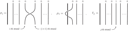
Figure 2. The generators of ${\rm Y}_{d,n}^{\mathtt{B}}(\mathsf{u},\mathsf{v})$.

Note.

For $d=1$, the algebra ${\rm Y}_{1,n}^{\mathtt{B}}$ coincides with ${\rm H}_{n}(\mathsf{u},\mathsf{v})$. By mapping $g_{i}\mapsto g_{i}$ and $t_{i}\mapsto 1$, we obtain an epimorphism from ${\rm Y}_{d,n}^{\mathtt{B}}$ to ${\rm H}_{n}(\mathsf{u},\mathsf{v})$. Moreover, if we map the $t_{i}$’s to a fixed non-trivial $d$-th root of the unity, we have an epimorphism from ${\rm Y}_{d,n}^{\mathtt{B}}$ to ${\rm H}_{n}(\mathsf{u},1)$.

In [10] two different linear bases for ${\rm Y}_{d,n}^{\mathtt{B}}$ are given, denoted by $\mathsf{D}_{n}$ and $\mathsf{C}_{n}$ respectively. We only recall the second one, since it is the one that is used in the definition of the Markov trace of ${\rm Y}_{d,n}^{\mathtt{B}}$. For all $1\leq k\leq n$, we define inductively the sets $M_{d,k}$ by:

$$M_{d,1}=\{t_{1}^{m},t_{1}^{m}b_{1}\,;\,0\leq m\leq d-1\}$$

and

$$M_{d,k}=\{t_{k}^{m},t_{k}^{m}b_{k},g_{k-1}x\,;\,x\in M_{d,k-1},\,0\leq m\leq d-1\}\quad\quad\mbox{for all $2\leq k\leq n$.}$$

where the elements $b_{k}$’s are as in Section 2.2. Define now $\mathsf{C}_{n}$ as the subset of ${\rm Y}_{d,n}^{\mathtt{B}}$ formed by the elements $\mathfrak{m}_{1}\mathfrak{m}_{2}\cdots\mathfrak{m}_{n}$, with $\mathfrak{m}_{i}\in M_{d,i}$. Moreover, every element of $M_{d,k}$ has the form $\mathfrak{m}_{k,j,m}^{+}$ or $\mathfrak{m}_{k,j,m}^{-}$ with $j\leq k$ and $0\leq m\leq d-1$, where

$$\mathfrak{m}_{k,k,m}^{+}:=t_{k}^{m},\qquad\mathfrak{m}_{k,j,m}^{+}:=g_{k-1}\cdots g_{j}t_{j}^{m}\quad\text{for}\ j<k,$$

and

$$\mathfrak{m}_{k,k,m}^{-}:=t_{k}^{m}b_{k},\qquad\mathfrak{m}_{k,j,m}^{-}:=g_{k-1}\cdots g_{j}b_{j}t_{j}^{m}\quad\text{for}\ j<k.$$

From the above, one can deduce that the basis $\mathsf{C}_{n}$ for ${\rm Y}_{d,n}^{\mathtt{B}}$ may be rewritten as follows [10, Proposition 5]):

(2.18) $$\mathsf{C}_{n}=\{t_{1}^{a_{1}}t_{2}^{a_{2}}\dots t_{n}^{a_{n}}m\ |\ m\in\mathtt{C}_{n},\ a_{i}\in\{0,\ldots,d-1\}\}.$$

In [10] Flores et al. proved that ${\rm Y}_{d,n}^{\mathtt{B}}$ supports a unique Markov trace. In brief, they construct a certain family of linear maps ${\rm tr}_{n}:{\rm Y}_{d,n}^{\mathtt{B}}\longrightarrow{\rm Y}_{d,n-1}^{\mathtt{B}}$, called relative traces, that build step by step the desired Markov properties (see also [4]). Finally, the Markov trace on ${\rm Y}_{d,n}^{\mathtt{B}}$ is defined by:

$${\rm Tr}_{n}:={\rm tr}_{1}\circ\cdots\circ{\rm tr}_{n}.$$

Theorem 1 (cf. Theorem 3 [10]).

Let $z,x_{1},\dots,x_{d-1},y_{0},\dots,y_{d-1}$ be indeterminates in $\mathbb{K}(z,x_{1},\dots,x_{d-1},$ $y_{0},\dots,y_{d-1})$ and let $x_{0}:=1$. Then the linear map ${\rm Tr}$ is a Markov trace on $\{{\rm Y}_{d,n}^{\mathtt{B}}\}_{n\geq 1}$. That is, for every $n\geq 1$, the linear map ${\rm Tr}_{n}:{\rm Y}_{d,n}^{\mathtt{B}}\longrightarrow\mathbb{K}(z,x_{1},\dots,x_{d-1},y_{0},\dots,y_{d-1})$ satisfies the following rules:

1. ${\rm Tr}_{n}(1)=1$,

2. ${\rm Tr}_{n+1}(Xg_{n})=z{\rm Tr}_{n}(X)$,

3. ${\rm Tr}_{n+1}(Xb_{n+1}t_{n+1}^{m})=y_{m}{\rm Tr}_{n}(X)$,

4. ${\rm Tr}_{n+1}(Xt_{n+1}^{m})=x_{m}{\rm Tr}_{n}(X)$,

5. ${\rm Tr}_{n}(XY)={\rm Tr}_{n}(YX),$

where $X,Y\in{\rm Y}_{d,n}^{\mathtt{B}}$.

Recall that the method of Jones for obtaining link invariants requires a rescaled and normalized Markov trace function. An interesting property of the trace ${\rm Tr}$ is that it does not rescale directly according to the framed braid equivalence for the solid torus. Indeed, the trace ${\rm Tr}$ can be rescaled only if the parameters $x_{i}$, $1\leq i\leq d-1$, are solutions of a non-linear system of equations that is called the ${\rm E}$-system [26, Appendix], while the parameters $y_{j}$, $0\leq j\leq d-1$, are solutions of an analogous non-linear system called the ${\rm F}$-system [10]. Consequently, new invariants for framed knots and links in the solid torus can be constructed, denoted by ${\mathcal{X}}_{S}^{\mathtt{B}}$, that are parametrized by $S\subseteq C_{d}$ (for more details see [10, Section 7]). The invariants ${\mathcal{X}}_{S}^{\mathtt{B}}$ when restricted to framed links with all framings equal to zero, give rise to invariants of oriented classical links in the solid torus. Since classical knot theory embeds in the knot theory of the solid torus and by using the results of [5], we deduce that the ${\mathcal{X}}_{S}^{\mathtt{B}}$ invariants are different than the invariant $P^{\mathtt{B}}(\mathsf{u},\mathsf{v},x,y)$ on links [11, 27].

2.4. The Framization of the Temperley-Lieb algebra of type $\mathtt{A}$

The framization of the Temperley-Lieb algebra of type $\mathtt{A}$ and the derived invariants for framed and classical links were studied extensively by Goundaroulis and collaborators [12, 13, 14]. As mentioned earlier, it is a well known fact that the Temperley-Lieb algebra of type $\mathtt{A}$ can be obtained as the quotient of the algebra ${\rm H}_{n}(u)$ modulo the two-sided ideal that is generated by the following elements:

$$g_{i,i+1}:=\sum_{w\in\langle s_{i},s_{i+1}\rangle}g_{w}.$$

Similarly, the framization of the Temperley-Lieb algebra of type $\mathtt{A}$ is defined as a quotient of the Yokonuma-Hecke algebra of type $\mathtt{A}$, which is denoted by ${\rm Y}_{d,n}(u)$ [21]. However, such a quotient is not unique in the case of framization. As mentioned in the introduction, the quotient algebra that eventually is chosen is the most natural with respect to the construction of new, non-trivial invariants for framed and classical knot and links.

The first quotient algebra that was studied is the Yokonuma-Temperley-Lieb algebra [13], denoted ${\rm YTL}_{d,n}(u)$, and proved to be too restrictive. As a consequence, basic pairs of framed links were not distinguished. For this reason this algebra was discarded as a potential candidate for the framization of the Temperley-Lieb algebra however, the Jones polynomial was recovered from this construction. The second candidate was the Complex Reflection Temperley-Lieb algebra, denoted ${\rm CTL}_{d,n}(u)$ [14]. In contrast to the case of ${\rm YTL}_{d,n}(u)$, the invariants that are derived from ${\rm CTL}_{d,n}(u)$ proved to coincide either with those from the algebra ${\rm Y}_{d,n}(u)$ or with those that are derived from the actual framization of the Temperley-Lieb algebra [14, Proposition 10]. This result is consistent with the fact that the algebra ${\rm CTL}_{d,n}(u)$ is isomorphic to a direct sum of matrix algebras over tensor products of Temperley-Lieb and Iwahori-Hecke algebras [6]. Thus, the quotient algebra ${\rm CTL}_{d,n}(u)$ is also discarded as a potential candidate for the framization of the Temperley-Lieb algebra.

The framization of the Temperley-Lieb algebra is an intermediate algebra between the algebras ${\rm YTL}_{d,n}(u)$ and ${\rm CTL}_{d,n}(u)$. It is denoted by ${\rm FTL}_{d,n}(u)$, and it is defined as the quotient of the algebra ${\rm Y}_{d,n}(u)$ modulo the two-sided ideal that is generated by the element:

$$r_{1,2}:=e_{1}e_{2}(1+g_{1}+g_{2}+g_{1}g_{2}+g_{2}g_{1}+g_{1}g_{2}g_{1}).$$

In [14, Theorem 6] necessary and sufficient conditions were determined so that the trace of ${\rm Y}_{d,n}(u)$ passes to ${\rm FTL}_{d,n}(u)$. These conditions led to a family of new 1-variable invariants for classical links, $\left\{\theta_{d}\right\}_{d\in\mathbb{N}}$, that are topologically not equivalent to the Jones polynomial on links, while they are topologically equivalent to the Jones polynomial on knots [14, Theorem 9]. Finally, the invariants $\theta_{d}(q)$ can be generalized to a 2-variable invariant for classical links, $\theta(q,E)$. More precisely, we have the following:

Theorem 2 ([15, Theorem 1.1]).

Let $q,E$ be indeterminates and let $\mathcal{L}$ be the set of all oriented links. There exists a unique ambient isotopy invariant of classical oriented links

$$\theta:\mathcal{L}\rightarrow\mathbb{C}[q^{\pm 1},E^{\pm 1}]$$

defined by the following rules:

1. On crossings involving different components the following skein relation holds:

   $$q^{-2}\,\theta(L_{+})-q^{2}\,\theta(L_{-})=(q-q^{-1})\,\theta(L_{0}),$$

   where $L_{+}$, $L_{-}$ and $L_{0}$ constitute a Conway triple.

2. For a union $\mathcal{K}=\sqcup_{i=1}^{r}K_{i}$ of $r$ unlinked knots, with $r\geq 1$, it holds that:

   $$\theta(\mathcal{K})=E^{1-r}V(\mathcal{K}),$$

   where $V(\mathcal{K})$ is the value of the Jones polynomial on $\mathcal{K}$.

The invariant $\theta(q,E)$ is topologically equivalent to the Jones polynomial on knots while it is stronger than the Jones polynomial on links [15, Theorem 5] (see Section 5.2).

3. The Temperley-Lieb algebra associated to the Coxeter group of type ${\mathtt{B}}$

We begin this section by defining the Temperley-Lieb algebra of type ${\mathtt{B}}$ as a quotient of the Hecke algebra of type $\mathtt{B}$. This is derived from the definition for an arbitrary Coxeter group [16].

As mentioned earlier, the classical Temperley-Lieb algebra can be expressed as a quotient of the Hecke algebra of type $\mathtt{A}$. Based on this, Fan and Green defined the Temperley-Lieb algebras associated to any simply laced Coxeter group [8]. This was done by first considering the Hecke algebra associated to the respective Coxeter group and then naturally extending the defining ideal of the classical case. Using the same procedure Green and Losonczy extended this definition to any Coxeter group [16]. Specifically, consider $(W,S)$ to be an arbitrary Coxeter System, and let $H(W)$ be the associated Hecke algebra. Then, the algebra $H(W)$ has a basis consisting of elements $T_{w}$, $w\in W$ that satisfy:

(3.1) $$T_{s}T_{w}=\left\{\begin{array}[]{lcl}T_{sw},&\mbox{if}&\ell(sw)>\ell(w)\\ a_{s}T_{sw}+b_{s}T_{w},&\mbox{if}&\ell(sw)<\ell(w)\end{array}\right.$$

where $\ell$ is the length function in $W$ and $a_{s}$, $b_{s}$ are parameters that depend on $s\in S$ such that $a_{s}=a_{t}$ and $b_{s}=b_{t}$ whenever $s$ and $t$ are conjugate in $W$. For further details the reader is referred to [17, Chapter 7]. Let now $J$ be the two-sided ideal of $H(W)$ that is generated by the following elements:

$$\sum_{w\in\langle s_{i},s_{j}\rangle}T_{w}$$

where $(s_{i},s_{j})$ runs over all pairs of $S$ that correspond to adjacent nodes in the Dynkin diagram of $W$. Then the generalized Temperley-Lieb algebra, ${\rm TL}(W)$, is defined as the quotient $H(W)/J$.

We shall specialize now the algebra ${\rm TL}(W)$ to the case of Coxeter systems of type $\mathtt{B}$. From the discussion above and by considering also the change of generators in Remark 1, we have that the defining two-sided ideal, denoted by $J_{B}$, is generated by the elements:

$$g_{i,i+1} = 1+\mathsf{u}(g_{i}+g_{i+1})+\mathsf{u}^{2}(g_{i}g_{i+1}+g_{i+1}g_{i})+\mathsf{u}^{3}g_{i}g_{i+1}g_{i}$$

$$g_{\mathtt{B}} := 1+\mathsf{u}g_{1}+\mathsf{v}b_{1}+\mathsf{u}\mathsf{v}(g_{1}b_{1}+b_{1}g_{1})+\mathsf{u}^{2}\mathsf{v}g_{1}b_{1}g_{1}+\mathsf{v}^{2}\mathsf{u}b_{1}g_{1}b_{1}$$

$$+(\mathsf{u}\mathsf{v})^{2}g_{1}b_{1}g_{1}b_{1},$$

where $1\leq i\leq n-2$. Given that the elements $g_{i,i+1}$ are all conjugates of $g_{1,2}$ in ${\rm H}_{n}(\mathsf{u},\mathsf{v})$ (see [13]), we conclude that $J_{B}=\langle g_{\mathtt{B}},g_{1,2}\rangle$.

Definition 1.

We define ${\rm TL}_{n}^{\mathtt{B}}:={\rm TL}_{n}^{\mathtt{B}}(\mathsf{u},\mathsf{v})$, the Temperley-Lieb algebra associated to the Coxeter group of type ${\mathtt{B}}$ as the quotient ${\rm H}_{n}(\mathsf{u},\mathsf{v})/J_{B}$.

3.1. A Markov trace on the algebra ${\rm TL}_{n}^{\mathtt{B}}$

The purpose of this section is to find the necessary and sufficient conditions such that the trace defined in ${\rm H}_{n}(\mathsf{u},\mathsf{v})$ passes to ${\rm TL}_{n}^{\mathtt{B}}$.

Let $W$ be a Coxeter group, and $H(W)$ the Hecke algebra associated to $W$. Now consider $b_{s}=a_{s}-1$ in (3.1) and set $x=\sum_{w\in W}T_{w}$. Observe that [28, Lemma 3.2] is valid for every finite Coxeter group, that is:

(3.2) $$xT_{s}=a_{s}x,\quad\hbox{for all $s\in S$}$$

Equation (3.2) and direct computations prove the following two lemmas.

Lemma 1.

The following holds in $H_{n}(\mathsf{u},\mathsf{v})$:

• $g_{1}g_{1,2}=g_{1,2}g_{1}=\mathsf{u}g_{1,2}$

• $g_{2}g_{1,2}=g_{1,2}g_{2}=\mathsf{u}g_{1,2}$

Lemma 2.

In ${\rm H}_{n}(\mathsf{u},\mathsf{v})$ the following equations holds

• $b_{1}g_{\mathtt{B}}=g_{\mathtt{B}}b_{1}=\mathsf{v}g_{\mathtt{B}}$

• $g_{1}g_{\mathtt{B}}=g_{\mathtt{B}}g_{1}=\mathsf{u}g_{\mathtt{B}}$

In analogy to ${\rm TL}_{n}(u)$, the trace ${\rm\tau}$ passes to the quotient ${\rm TL}_{n}^{\mathtt{B}}$ if and only if ${\rm\tau}$ annihilates the defining ideal $\langle g_{1,2},g_{\mathtt{B}}\rangle$ of ${\rm TL}_{n}^{\mathtt{B}}$:

(3.3) $${\rm\tau}(mg_{\mathtt{B}})+{\rm\tau}(ng_{1,2})=0,$$

where $m,n$ are in the linear basis of ${\rm H}_{n}(\mathsf{u},\mathsf{v})$. We shall determine now the necessary and sufficient conditions so that (3.3) holds. We will use induction on $n$. We start with the following lemma:

Lemma 3.

The following hold in ${\rm H}_{n}(\mathsf{u},\mathsf{v})$:

$${\rm\tau}(g_{1,2}) =(\mathsf{u}^{2}+1)(\mathsf{u}z)^{2}+(\mathsf{u}^{2}+2)\mathsf{u}z+1$$

$${\rm\tau}(g_{\mathtt{B}}) =\mathsf{u}^{2}\mathsf{v}^{2}y^{2}+(\mathsf{u}\mathsf{v}+\mathsf{u}^{3}\mathsf{v}^{3})zy+(\mathsf{v}+\mathsf{u}^{2}\mathsf{v})y+(\mathsf{u}+\mathsf{u}^{3}\mathsf{v}^{2})z+1$$

Proof.

The proof follows immediately from the defining rules of ${\rm\tau}$. ∎

We shall treat each summand of (3.3) separately. For the first summand we have the following:

Proposition 1.

For all $m\in{\rm H}_{n}(\mathsf{u},\mathsf{v})$ we have that

$${\rm\tau}(mg_{\mathtt{B}})=p(\mathsf{u},\mathsf{v},z,y){\rm\tau}(g_{\mathtt{B}}),\quad\text{for all $n\geq 2$}$$

where $p(\mathsf{u},\mathsf{v},z,y)$ is a monomial in the variables $\mathsf{u},\mathsf{v},z,y$.

Proof.

By linearity of the trace, it is enough to prove the statement for an element $m$ in the inductive basis $\mathtt{C}_{n}$. We will proceed by induction. For $n=2$ the result follows directly by Lemma 2. Suppose now that the argument holds for any $w\in{\rm H}_{n}(\mathsf{u},\mathsf{v})$, and let $m\in{\rm H}_{n+1}(\mathsf{u},\mathsf{v})$, where $m=wb_{n+1}$ or $m=wg_{n}\dots g_{i}b_{i}^{a}$, with $a=0,1$ and $w\in{\rm H}_{n}(\mathsf{u},\mathsf{v})$. We have that

$${\rm\tau}(wb_{n+1}) = y{\rm\tau}(w)$$

$${\rm\tau}(wg_{n}\dots g_{i}b_{i}^{a}) = z{\rm\tau}(\alpha)$$

where $\alpha=wg_{n-1}\dots g_{i}b_{i}^{a}\in{\rm H}_{n}(\mathsf{u},\mathsf{v})$ and so the result follows by the induction hypothesis. ∎

Lemma 4.

For $i\geq 1$ we have that

$${\rm\tau}(b_{i}g_{1,2})=y{\rm\tau}(g_{1,2})$$

Proof.

First note that ${\rm\tau}(b_{1}g_{1,2})=y{\rm\tau}(g_{1,2})$ follows easily by the trace rules, since $b_{1}\in{\rm H}_{1}(\mathsf{u},\mathsf{v})$. For $i=2$ we have that

$${\rm\tau}(b_{2}g_{1,2})={\rm\tau}(g_{1}b_{1}g_{1}^{-1}g_{1,2}).$$

From Lemma 1 we obtain

$${\rm\tau}(g_{1}b_{1}g_{1}^{-1}g_{1,2})=\mathsf{u}^{-1}{\rm\tau}(g_{1}b_{1}g_{1,2})=\mathsf{u}^{-1}{\rm\tau}(b_{1}g_{1,2}g_{1})={\rm\tau}(b_{1}g_{1,2})=y{\rm\tau}(g_{1,2}).$$

The case $i=3$ is completely analogous, while for $i\geq 4$ the result follows immediately by the trace rules. ∎

The following proposition deals with the second term of (3.3).

Proposition 2.

Let $n\geq 3$. For all $m\in{\rm H}_{n}(\mathsf{u},\mathsf{v})$ we have that

(3.4) $${\rm\tau}(mg_{1,2})=\left\{\begin{array}[]{l}p(\mathsf{u},\mathsf{v},z,y){\rm\tau}(g_{1,2})\\ p(\mathsf{u},\mathsf{v},z,y){\rm\tau}(b_{1}g_{1}b_{1}g_{1,2})\\ p(\mathsf{u},\mathsf{v},z,y){\rm\tau}(b_{1}g_{1}b_{1}g_{2}g_{1}b_{1}g_{1,2})\end{array}\right.$$

where $p(\mathsf{u},\mathsf{v},z,y)$ is a monomial in the variables $\mathsf{u},\mathsf{v},z,y$.

Proof.

Since $\tau$ is linear, it’s enough to prove (3.4) for any $m$ in the basis $\mathsf{C}_{n}$ from ${\rm H}_{n}(\mathsf{u},\mathsf{v})$. Again, we will use induction on $n$. We start by proving that the argument holds for $n=3$. First note that

$$\mathsf{C}_{2}=\{1,b_{2},g_{1},g_{1}b_{1},b_{1},b_{1}b_{2},b_{1}g_{1},b_{1}g_{1}b_{1}\}$$

From Lemmas 4 and 1 we have that

$$\begin{array}[]{rclrcl}{\rm\tau}(b_{2}g_{1,2})&=&y{\rm\tau}(g_{1,2});&{\rm\tau}(g_{1}g_{1,2})&=&\mathsf{u}{\rm\tau}(g_{1,2})\\ {\rm\tau}(g_{1}b_{1}g_{1,2})&=&\mathsf{u}y{\rm\tau}(g_{1,2});&{\rm\tau}(b_{1}g_{1,2})&=&y{\rm\tau}(g_{1,2})\\ {\rm\tau}(b_{1}g_{1}g_{1,2})&=&\mathsf{u}y{\rm\tau}(g_{1,2});&{\rm\tau}(b_{1}b_{2}g_{1,2})&=&\mathsf{u}^{-1}{\rm\tau}(b_{1}g_{1}b_{1}g_{1,2})\end{array}$$

Suppose now that $m\in C_{3}$. This means that $m=wm_{3}$ for some $w\in\mathsf{C}_{2}$ and $m_{3}\in\{g_{2}g_{1}b_{1},g_{2}b_{2},b_{3},g_{2}g_{1},g_{2},1\}$. From the previous results and Lemma 1 we obtain that

$$\begin{array}[]{rclrcl}{\rm\tau}(wg_{2}b_{2}g_{1,2})&=&\mathsf{u}^{-1}{\rm\tau}(wg_{2}g_{1}b_{1}g_{1,2});&{\rm\tau}(wb_{3}g_{1,2})&=&\mathsf{u}^{-2}{\rm\tau}(wg_{2}g_{1}b_{1}g_{1,2})\\ {\rm\tau}(wg_{2}g_{1}g_{1,2})&=&\mathsf{u}^{2}{\rm\tau}(wg_{1,2});&{\rm\tau}(wg_{2}g_{1,2})&=&\mathsf{u}{\rm\tau}(wg_{1,2})\end{array}$$

Therefore, we only have to study ${\rm\tau}(wg_{2}g_{1}b_{1}g_{1,2})$. Replacing $w$ and by applying previous lemmas and using the trace rules on each element in $\mathsf{C}_{2}$, we have:

$$\begin{array}[]{rclrcl}{\rm\tau}(g_{2}g_{1}b_{1}g_{1,2})&=&\mathsf{u}^{2}y{\rm\tau}(g_{1,2});&{\rm\tau}(b_{2}g_{2}g_{1}b_{1}g_{1,2})&=&\mathsf{u}{\rm\tau}(b_{1}g_{1}b_{1}g_{1,2})\\ {\rm\tau}(g_{1}g_{2}g_{1}b_{1}g_{1,2})&=&\mathsf{u}^{3}y{\rm\tau}(g_{1,2});&{\rm\tau}(g_{1}b_{1}g_{2}g_{1}b_{1}g_{1,2})&=&\mathsf{u}^{2}{\rm\tau}(b_{1}g_{1}b_{1}g_{1,2})\\ {\rm\tau}(b_{1}g_{2}g_{1}b_{1}g_{1,2})&=&\mathsf{u}{\rm\tau}(b_{1}g_{1}b_{1}g_{1,2});&{\rm\tau}(b_{1}g_{1}g_{2}g_{1}b_{1}g_{1,2})&=&\mathsf{u}^{2}{\rm\tau}(b_{1}g_{1}b_{1}g_{1,2})\end{array}$$

$${\rm\tau}(b_{1}b_{2}g_{2}g_{1}b_{1}g_{1,2})=\mathsf{u}^{-1}{\rm\tau}(b_{1}g_{1}b_{1}g_{2}g_{1}b_{1}g_{1,2})$$

From the above, the result follows for $n=3$. Finally, suppose that the argument holds for $m\in{\rm H}_{n}(\mathsf{u},\mathsf{v})$ and let $m\in{\rm H}_{n+1}(\mathsf{u},\mathsf{v})$. We have that $m=wb_{n+1}$ or $m=wg_{n}\dots g_{i}b_{i}^{a}$, with $a=0,1$ and $w\in{\rm H}_{n}(\mathsf{u},\mathsf{v})$. Since we have that

$${\rm\tau}(wb_{n+1}) = y{\rm\tau}(w)$$

$${\rm\tau}(wg_{n}\dots g_{i}b_{i}^{a}) = z{\rm\tau}(\alpha),\quad\text{where $\alpha=wg_{n-1}\dots g_{i}b_{i}^{a}\in{\rm H}_{n}(\mathsf{u},\mathsf{v})$}$$

then result follows by the induction hypothesis. ∎

The discussion above suggests that (3.3) reduces to a homogenous system of four equations of the trace parameters $z$ and $y$, namely:

Theorem 3.

The following statements are equivalent

• ${\rm\tau}(mg_{1,2})+{\rm\tau}(ng_{\mathtt{B}})=0\quad\text{for all $m,n\in{\rm H}_{n}(\mathsf{u},\mathsf{v})$}$

• ${\rm\tau}(g_{\mathtt{B}})={\rm\tau}(g_{1,2})={\rm\tau}(b_{1}g_{1}b_{1}g_{1,2})={\rm\tau}(b_{1}g_{1}b_{1}g_{2}g_{1}b_{1}g_{1,2})=0$

Proof.

Since (i) holds for all $m,n\in{\rm H}_{n}(\mathsf{u},\mathsf{v})$, then it must also hold for $m=1$ and $n=0$. Thus, we deduce argument (ii). The converse is a direct consequence of Propositions 1 and 2. ∎

The following lemma will be used in the proof of Theorem 4 below. We have that:

Lemma 5.

The following equations hold:

$$\begin{array}[]{l l c l }(i)&\tau(b_{1}g_{1}b_{1}g_{1,2})&=&\mathsf{v}^{-1}\left(\mathsf{u}(1+\mathsf{u}z+\mathsf{u}^{3}z)(\mathsf{v}y^{2}+\mathsf{u}(\mathsf{v}+(\mathsf{v}^{2}-1)y)z)\right)\\ (ii)&\tau(b_{1}g_{1}b_{1}g_{2}g_{1}b_{1}g_{1,2})&=&\mathsf{v}^{-2}\left(\mathsf{u}^{3}(\mathsf{v}^{2}y^{3}+\mathsf{u}(2+\mathsf{u}^{2})\mathsf{v}y(\mathsf{v}+(\mathsf{v}^{2}-1)y)z\right.\\ &&&\left.+\mathsf{u}^{2}(1+\mathsf{u}^{2})(y+\mathsf{v}(\mathsf{v}^{2}-1)(1+\mathsf{v}y))z^{2}\right)\end{array}$$

Proof.

The proof is a long straightforward computation using the rules of $\tau$. ∎

We are now able to give the necessary and sufficient conditions for $\tau$ to pass to ${\rm TL}_{n}^{\mathtt{B}}(\mathsf{u},\mathsf{v})$. Indeed, we have:

Theorem 4.

The trace $\tau$ passes to the quotient algebra ${\rm TL}_{n}^{\mathtt{B}}(\mathsf{u},\mathsf{v})$ if and only if the trace parameters $z$ and $y$ take one of the following values.

• $z=-\frac{1}{\mathsf{u}}$ and $y=-\frac{1}{\mathsf{v}}$,                (ii) $z=-\frac{1}{\mathsf{u}}$ and $y=\mathsf{v}$,

• $z=-\frac{1}{\mathsf{u}(1+\mathsf{u}^{2})}$ and $y=-\frac{1}{\mathsf{v}}$,   (iv)  $z=-\frac{1}{\mathsf{u}(1+\mathsf{u}^{2})}$ and $y=\frac{-1+\mathsf{v}^{2}}{(1+\mathsf{u}^{2})\mathsf{v}}$.

Proof.

From Theorem 3 we have that $\tau$ annihilates the ideal $J$ if and only if the following system of equations has solutions for $z$ and $y$:

$$(\Sigma):=\ \left\{\begin{aligned} &{\rm\tau}(g_{\mathtt{B}})=0\\ &{\rm\tau}(g_{1,2})=0\\ &{\rm\tau}(b_{1}g_{1}b_{1}g_{1,2})=0\\ &{\rm\tau}(b_{1}g_{1}b_{1}g_{2}g_{1}b_{1}g_{1,2})=0\end{aligned}\right.$$

Using Lemmas 3 and 5 one can derive the four sets of solutions for $(\Sigma)$ and, therefore, the necessary and sufficient conditions for the passing of $\tau$ to ${\rm TL}_{n}^{\mathtt{B}}$. ∎

3.2. Link invariants from ${\rm TL}_{n}^{\mathtt{B}}(\mathsf{u},\mathsf{v})$

Following Jones [19], we can now define link invariants in the solid torus. Starting from (2.5), we specialize the parameters $z,y$ to the necessary and sufficient conditions of Theorem 4. Note that the values $z=-1/\mathsf{u}$, $y=-1/\mathsf{v}$ and $y=-\mathsf{v}$ are discarded since they are of no topological interest [19, Section 11]. From the remaining pair of values $z=-\frac{1}{\mathsf{u}(1+\mathsf{u}^{2})}$ and $y=\frac{\mathsf{v}^{2}-1}{(1+\mathsf{u}^{2})\mathsf{v}}$ we deduce that $\lambda=\mathsf{u}^{4}$ and thus we have:

Definition 2.

The following is an invariant for links inside the solid torus

(3.5) $$V^{\mathtt{B}}(\mathsf{u},\mathsf{v}):=\left(-\frac{1+\mathsf{u}^{2}}{\mathsf{u}}\right)^{n-1}\mathsf{u}^{2\varepsilon(\alpha)}\tau(\overline{\pi}(\alpha)),$$

where $\alpha$, $\widehat{\alpha}$, $\varepsilon(\alpha)$ are as in (2.5) and $\overline{\pi}$ is the natural epimorphism $\widetilde{W}_{n}\rightarrow{\rm TL}_{n}^{\mathtt{B}}(\mathsf{u},\mathsf{v})$ sending $\sigma_{i}\mapsto g_{i}$ and $r_{1}\mapsto b_{1}$.

Remark 2.

By substituting $\lambda=\mathsf{u}^{4}$ in (2.6) and (2.7) we derive that $V^{\mathtt{B}}$ can be defined completely by the following skein relations:

(3.6) $$\mathsf{u}^{-2}\ V^{\mathtt{B}}(L_{+})-\mathsf{u}^{2}\ V^{\mathtt{B}}(L_{-}) =\left(\mathsf{u}-\mathsf{u}^{-1}\right)V^{\mathtt{B}}(L_{0})$$

(3.7) $$V^{\mathtt{B}}(M_{+})-V^{\mathtt{B}}(M_{-}) =\left(\mathsf{v}-\mathsf{v}^{-1}\right)V^{\mathtt{B}}(M_{0}),$$

where $L_{+}$, $L_{-}$, $L_{0}$, $M_{+}$ , $M_{-}$ and $M_{0}$ are as shown in Fig. 1.

4. Framization of the Temperley-Lieb algebra associated to the Coxeter group of type ${\mathtt{B}}$

In this section we introduce ${\rm FTL}_{d,n}^{\mathtt{B}}$, the framization of the Temperley-Lieb algebra associated to the Coxeter group of type ${\mathtt{B}}$. This extends naturally the work done for the type ${\mathtt{A}}$ case in [14]. In more detail, the framization will be defined as a quotient of the algebra ${\rm Y}_{d,n}^{\mathtt{B}}$ modulo an appropriate two-sided ideal. Since the algebra ${\rm Y}_{d,n}(u)$ is contained in ${\rm Y}_{d,n}^{\mathtt{B}}$, following Section 2.4 we consider the following element in ${\rm Y}_{d,n}^{\mathtt{B}}(\mathsf{u},\mathsf{v})$:

(4.1) $$r_{1,2}:=e_{1}e_{2}g_{1,2}.$$

The element $r_{1,2}$ is the generator of the type $\mathtt{A}$ part of the quotient algebra ${\rm FTL}_{d,n}^{\mathtt{B}}$. Accordingly, we consider also the generator of the type $\mathtt{B}$ part, which is the element:

$$r_{{\mathtt{B}}}:=f_{1}e_{1}g_{\mathtt{B}}$$

Definition 3.

The framization of the Temperley-Lieb algebra associated to the Coxeter group of type ${\mathtt{B}}$ is defined as follows:

(4.2) $${\rm FTL}_{d,n}^{\mathtt{B}}(\mathsf{u},\mathsf{v}):={\rm Y}_{d,n}^{\mathtt{B}}(\mathsf{u},\mathsf{v})/\langle r_{{\mathtt{B}}},r_{1,2}\rangle$$

We give below the framed analogues of Lemmas 1 and 2 that will be used extensively later.

Lemma 6.

The following holds in ${\rm Y}_{d,n}^{\mathtt{B}}(\mathsf{u},\mathsf{v})$:

• $g_{1}r_{1,2}=r_{1,2}g_{1}=\mathsf{u}r_{1,2}$

• $g_{2}r_{1,2}=r_{1,2}g_{2}=\mathsf{u}r_{1,2}$

Proof.

The proof follows from a straightforward computation. For demonstrative reasons, we only prove the case $r_{1,2}g_{1}$. Observe that the element $e_{1}e_{2}$ commutes with $g_{1}$ and $g_{2}$. On the other hand, we also have that

(4.3) $$e_{i}g_{i}^{2}=e_{i}(1+(\mathsf{u}-\mathsf{u}^{-1})e_{i}g_{i})=e_{i}(1+(\mathsf{u}-\mathsf{u}^{-1})g_{i}).$$

The result follows from (4.3) and by using Lemma 1. ∎

We will prove now that an analogous result holds for the generator of the $\mathtt{B}$-type case.

Lemma 7.

In ${\rm Y}_{d,n}^{\mathtt{B}}(\mathsf{u},\mathsf{v})$ the following equations holds

• $b_{1}r_{{\mathtt{B}}}=r_{{\mathtt{B}}}b_{1}=\mathsf{v}r_{{\mathtt{B}}}$

• $g_{1}r_{{\mathtt{B}}}=r_{{\mathtt{B}}}g_{1}=\mathsf{u}r_{{\mathtt{B}}}$

Proof.

We only prove the left multiplication for the first case. The proof for the second case is analogous. Similarly to the previous case, we have that the element $f_{1}f_{2}$ commutes with $b_{1}$ and $g_{1}$. Note now that the following equation holds in ${\rm Y}_{d,n}^{\mathtt{B}}(\mathsf{u},\mathsf{v})$:

$$f_{1}b_{1}^{2}=f_{1}(1+(\mathsf{v}-\mathsf{v}^{-1})f_{1}b_{1})=f_{1}(1+(\mathsf{v}-\mathsf{v}^{-1})b_{1}).$$

The result follows by using Lemma 2. ∎

4.1. Technical lemmas

Our next goal is to determine the necessary and sufficient conditions so that the trace ${\rm Tr}$ of ${\rm Y}_{d,n}^{\mathtt{B}}(\mathsf{u},\mathsf{v})$ in [10] passes to ${\rm FTL}^{\mathtt{B}}_{d,n}$. Our approach will be analogous to [14]. However, we need to postpone this discussion until the next subsection in order to present here a series of technical results that are required for the proof of our main theorem.

Lemma 8.

The following holds in ${\rm Y}_{d,n}^{\mathtt{B}}(\mathsf{u},\mathsf{v})$.

(4.4) $$1. \ {\rm Tr}(r_{\mathtt{B}})=\frac{1}{d^{2}}\sum_{r,s}x_{r}x_{s}+\mathsf{u}^{2}\mathsf{v}^{2}\frac{1}{d^{2}}\sum_{r,s}y_{r}y_{s}+\mathsf{v}(\mathsf{u}^{2}+1)\frac{1}{d^{2}}\sum_{r,s}x_{s}y_{r}.$$

$$\hskip 71.13188pt+z\mathsf{u}[1+\mathsf{u}^{2}\mathsf{v}^{2}]\frac{1}{d}\sum_{r}x_{r}+z[\mathsf{u}^{3}\mathsf{v}^{3}+\mathsf{u}\mathsf{v}]\frac{1}{d}\sum_{r}y_{r}$$

(4.5) $$2. \ {\rm Tr}({r_{1,2}})=(u+1)z^{2}x_{m}+(u+2)z\,E^{(m)}+{\rm tr}(e_{1}^{(m)}e_{2}).$$

Proof.

For the first argument we have that:

$${\rm Tr}(r_{\mathtt{B}})= \frac{1}{d^{2}}\sum_{r,s}x_{r}x_{s}+\mathsf{v}\frac{1}{d^{2}}\sum_{r,s}x_{s}y_{r}+z\mathsf{u}\frac{1}{d}\sum_{r}x_{r}+2z\mathsf{u}\mathsf{v}\frac{1}{d}\sum_{r}y_{r}+z\mathsf{v}^{2}\mathsf{u}\frac{1}{d}\sum_{r}x_{r}$$

$$+z\mathsf{v}^{2}\mathsf{u}(\mathsf{v}-\mathsf{v}^{-1})\frac{1}{d}\sum_{r}y_{r}+\mathsf{u}^{2}\mathsf{v}\frac{1}{d^{2}}\sum_{r,s}x_{r}y_{s}+z\mathsf{u}^{2}\mathsf{v}(\mathsf{u}-\mathsf{u}^{-1})\frac{1}{d}\sum_{r}y_{r}$$

$$+\mathsf{u}^{2}\mathsf{v}^{2}\frac{1}{d^{2}}\sum_{r,s}y_{r}y_{s}+z\mathsf{u}^{2}\mathsf{v}^{2}(\mathsf{u}-\mathsf{u}^{-1})\frac{1}{d}\sum_{r}x_{r}+z\mathsf{u}^{2}\mathsf{v}^{2}(\mathsf{u}-\mathsf{u}^{-1})(\mathsf{v}-\mathsf{v}^{-1})\frac{1}{d}\sum_{r}y_{r}$$

$$= \frac{1}{d^{2}}\sum_{r,s}x_{r}x_{s}+\mathsf{u}^{2}\mathsf{v}^{2}\frac{1}{d^{2}}\sum_{r,s}y_{r}y_{s}+(\mathsf{u}^{2}\mathsf{v}+\mathsf{v})\frac{1}{d^{2}}\sum_{r,s}x_{s}y_{r}+$$

$$z\left[\mathsf{u}+\mathsf{v}^{2}\mathsf{u}+\mathsf{v}^{2}\mathsf{u}^{2}(\mathsf{u}-\mathsf{u}^{-1})\right]\frac{1}{d}\sum_{r}x_{r}+z\left[2\mathsf{u}\mathsf{v}+\mathsf{u}^{2}\mathsf{v}(\mathsf{u}-\mathsf{u}^{-1})+\mathsf{u}\mathsf{v}^{2}(\mathsf{v}-\mathsf{v}^{-1})\right.$$

$$+\left.\mathsf{u}^{2}\mathsf{v}^{2}(\mathsf{u}-\mathsf{u}^{-1})(\mathsf{v}-\mathsf{v}^{-1})\right]\frac{1}{d}\sum_{r}y_{r}.$$

$$= \frac{1}{d^{2}}\sum_{r,s}x_{r}x_{s}+\mathsf{u}^{2}\mathsf{v}^{2}\frac{1}{d^{2}}\sum_{r,s}y_{r}y_{s}+\mathsf{v}(\mathsf{u}^{2}+1)\frac{1}{d^{2}}\sum_{r,s}x_{s}y_{r}+z\mathsf{u}[1+\mathsf{u}^{2}\mathsf{v}^{2}]\frac{1}{d}\sum_{r}x_{r}$$

$$+z[\mathsf{u}^{3}\mathsf{v}^{3}+\mathsf{u}\mathsf{v}]\frac{1}{d}\sum_{r}y_{r}.$$

For the second part of the proof the reader is referred to [14, Lemma 7]. ∎

The following two propositions show how ${\rm Tr}$ behaves on the elements of the defining ideal of ${\rm FTL}^{\mathtt{B}}(\mathsf{u},\mathsf{v})$. We start by exploring the case of the elements that involve the $\mathtt{B}$-type part of the algebra.

Proposition 3.

For all $m\in{\rm Y}_{d,n}^{\mathtt{B}}$ we have that

$${\rm Tr}(mr_{\mathtt{B}})=p(\mathsf{u},\mathsf{v},z,y_{a},x_{b}){\rm Tr}(r_{\mathtt{B}}),\quad\text{for all $n\geq 2$,}$$

where $p(\mathsf{u},\mathsf{v},z,y_{a},x_{b})$ is a monomial in the variables $\mathsf{u},\mathsf{v},z,y_{a}$ and $x_{b}$, with $0\leq a,b\leq d-1$.

Proof.

By the linearity of the trace, it is enough to prove the statement for an element $m$ in the inductive basis $\mathsf{C}_{n}$. We will proceed by induction. For $n=2$ the result follows from Lemma 7, and the fact that element $f_{1}f_{2}$ absorbs the framing part of $m$. For instance, if $m=t_{1}^{a}t_{2}^{b}b_{1}g_{1}b_{1}$ we have

$${\rm Tr}(mr_{\mathtt{B}})={\rm Tr}(t_{1}^{a}t_{2}^{b}b_{1}g_{1}b_{1}f_{1}f_{2}g_{\mathtt{B}})=\mathsf{v}^{2}\mathsf{u}{\rm Tr}(t_{1}^{a}t_{2}^{b}f_{1}f_{2}g_{\mathtt{B}})=\mathsf{v}^{2}\mathsf{u}{\rm Tr}(f_{1}f_{2}g_{\mathtt{B}}).$$

Suppose now that the argument holds for any $w\in{\rm Y}_{d,n-1}^{\mathtt{B}}$, and let $m\in{\rm Y}_{d,n}^{\mathtt{B}}$. Then, the element $m$ can be written as follows:

$$m=wt_{n}^{b}b_{n}^{a}\quad\text{or}\quad m=wg_{n-1}\dots g_{i}b_{i}^{a}t_{i}^{b},$$

with $w\in{\rm Y}_{d,n-1}^{\mathtt{B}}$, $a=0,1$ and $0\leq b\leq d-1$ . Since we have that

$${\rm Tr}(wt_{n}^{a}b_{n}) = y_{a}{\rm Tr}(w)$$

$${\rm Tr}(wt_{n}^{a}) = x_{a}{\rm Tr}(w)$$

$${\rm Tr}(wg_{n-1}\dots g_{i}b_{i}^{a}t_{i}^{b}) = z{\rm Tr}(\alpha),\quad\text{where $\alpha=wg_{n-2}\dots g_{i}b_{i}^{a}t_{i}^{b}\in{\rm H}_{n}(\mathsf{u},\mathsf{v})$}$$

the result follows by the induction hypothesis. ∎

The next proposition deals with the $\mathtt{A}$-type part of the algebra.

Proposition 4.

Let $n\geq 3$. For all $m\in{\rm Y}_{d,n}^{\mathtt{B}}$ we have that

(4.6) $${\rm Tr}(mr_{1,2})=\left\{\begin{array}[]{l}p(\mathsf{u},\mathsf{v},z,y_{a},x_{b}){\rm Tr}(t_{1}^{a}t_{2}^{b}t_{3}^{c}r_{1,2})\\ p(\mathsf{u},\mathsf{v},z,y_{a},x_{b}){\rm Tr}(t_{1}^{a}t_{2}^{b}t_{3}^{c}b_{1}r_{1,2})\\ p(\mathsf{u},\mathsf{v},z,y_{a},x_{b}){\rm Tr}(t_{1}^{a}t_{2}^{b}t_{3}^{c}b_{1}g_{1}b_{1}r_{1,2})\\ p(\mathsf{u},\mathsf{v},z,y_{a},x_{b}){\rm Tr}(t_{1}^{a}t_{2}^{b}t_{3}^{c}b_{1}g_{1}b_{1}g_{2}g_{1}b_{1}r_{1,2})\end{array}\right.$$

where $p(\mathsf{u},\mathsf{v},z,y_{a},x_{b})$ is a monomial in the variables $\mathsf{u},\mathsf{v},z,y_{a}$ and $x_{b}$, with $0\leq a,b\leq d-1$.

Proof.

The trace ${\rm Tr}$ is linear so it suffices to prove (4.6) for any $m$ in the basis $\mathsf{C}_{n}$ of ${\rm Y}_{d,n}^{\mathtt{B}}$. We will use again induction on $n$. We start by proving that the argument holds for $n=3$. Note that from Lemmas 7 and 6 we have:

$${\rm Tr}(t_{1}^{a}t_{2}^{b}t_{3}^{c}b_{2}r_{1,2})={\rm Tr}(t_{1}^{a}t_{2}^{b}t_{3}^{c}b_{1}r_{1,2});\quad{\rm Tr}(t_{1}^{a}t_{2}^{b}t_{3}^{c}b_{1}b_{2}r_{1,2})=\mathsf{u}^{-1}{\rm Tr}(t_{1}^{a}t_{2}^{b}t_{3}^{c}b_{1}g_{1}b_{1}r_{1,2})$$

$${\rm Tr}(t_{1}^{a}t_{2}^{b}t_{3}^{c}g_{1}b_{1}r_{1,2})=\mathsf{u}y{\rm Tr}(t_{1}^{a}t_{2}^{b}t_{3}^{c}b_{1}r_{1,2});\quad{\rm Tr}(t_{1}^{a}t_{2}^{b}t_{3}^{c}b_{1}g_{1}r_{1,2})=\mathsf{u}y{\rm Tr}(t_{1}^{a}t_{2}^{b}t_{3}^{c}b_{1}r_{1,2})$$

$${\rm Tr}(t_{1}^{a}t_{2}^{b}t_{3}^{c}g_{1}r_{1,2})=\mathsf{u}{\rm Tr}(t_{1}^{a}t_{2}^{b}t_{3}^{c}r_{1,2})$$

Next, suppose that $m\in\mathsf{C}_{3}$. This means that $m=t_{1}^{a}t_{2}^{b}t_{3}^{c}wm_{3}$ for some $w\in\mathtt{C}_{2}$ and $m_{3}\in\{g_{2}g_{1}b_{1},g_{2}b_{2},b_{3},g_{2}g_{1},g_{2},1\}$. From the previous results and from Lemma 6 we obtain the following:

$${\rm Tr}(t_{1}^{a}t_{2}^{b}t_{3}^{c}wg_{2}b_{2}r_{1,2})=\mathsf{u}^{-1}{\rm Tr}(t_{1}^{a}t_{2}^{b}t_{3}^{c}wg_{2}g_{1}b_{1}r_{1,2})$$

$${\rm Tr}(t_{1}^{a}t_{2}^{b}t_{3}^{c}wg_{2}g_{1}r_{1,2})=\mathsf{u}^{2}{\rm Tr}(t_{1}^{a}t_{2}^{b}t_{3}^{c}wr_{1,2})$$

$${\rm Tr}(t_{1}^{a}t_{2}^{b}t_{3}^{c}wb_{3}r_{1,2})=\mathsf{u}^{-2}{\rm Tr}(t_{1}^{a}t_{2}^{b}t_{3}^{c}wg_{2}g_{1}b_{1}r_{1,2})$$

$${\rm Tr}(t_{1}^{a}t_{2}^{b}t_{3}^{c}wg_{2}r_{1,2})=\mathsf{u}{\rm Tr}(t_{1}^{a}t_{2}^{b}t_{3}^{c}wr_{1,2})$$

Therefore, we only have to study the term ${\rm Tr}(t_{1}^{a}t_{2}^{b}t_{3}^{c}wg_{2}g_{1}b_{1}r_{1,2})$. Replacing $w$ for each element in $\mathtt{C}_{2}$ and by using previous lemmas and results, we obtain the following:

$${\rm Tr}(t_{1}^{a}t_{2}^{b}t_{3}^{c}g_{2}g_{1}b_{1}r_{1,2})=\mathsf{u}^{2}y{\rm Tr}(t_{1}^{a}t_{2}^{b}t_{3}^{c}b_{1}r_{1,2})$$

$${\rm Tr}(t_{1}^{a}t_{2}^{b}t_{3}^{c}b_{2}g_{2}g_{1}b_{1}r_{1,2})=\mathsf{u}{\rm Tr}(t_{1}^{a}t_{2}^{b}t_{3}^{c}b_{1}g_{1}b_{1}r_{1,2})$$

$${\rm Tr}(t_{1}^{a}t_{2}^{b}t_{3}^{c}g_{1}g_{2}g_{1}b_{1}r_{1,2})=\mathsf{u}^{3}y{\rm Tr}(t_{1}^{a}t_{2}^{b}t_{3}^{c}b_{1}r_{1,2})$$

$${\rm Tr}(t_{1}^{a}t_{2}^{b}t_{3}^{c}g_{1}b_{1}g_{2}g_{1}b_{1}r_{1,2})=\mathsf{u}^{2}{\rm Tr}(t_{1}^{a}t_{2}^{b}t_{3}^{c}b_{1}g_{1}b_{1}r_{1,2})$$

$${\rm Tr}(t_{1}^{a}t_{2}^{b}t_{3}^{c}b_{1}g_{2}g_{1}b_{1}r_{1,2})=\mathsf{u}{\rm Tr}(t_{1}^{a}t_{2}^{b}t_{3}^{c}b_{1}g_{1}b_{1}r_{1,2})$$

$${\rm Tr}(t_{1}^{a}t_{2}^{b}t_{3}^{c}b_{1}g_{1}g_{2}g_{1}b_{1}r_{1,2})=\mathsf{u}^{2}{\rm Tr}(t_{1}^{a}t_{2}^{b}t_{3}^{c}b_{1}g_{1}b_{1}r_{1,2})$$

$${\rm Tr}(t_{1}^{a}t_{2}^{b}t_{3}^{c}b_{1}b_{2}g_{2}g_{1}b_{1}r_{1,2})=\mathsf{u}^{-1}{\rm Tr}(t_{1}^{a}t_{2}^{b}t_{3}^{c}b_{1}g_{1}b_{1}g_{2}g_{1}b_{1}r_{1,2})$$

The result for $n=3$ follows immediately. Finally, we suppose that the argument holds for $w\in\mathtt{C}_{n-1}$, and let $m\in\mathtt{C}_{n}$. We have that $m^{(a)}=t_{1}^{a_{1}}\dots t_{n}^{a_{n}}wb_{n}^{a}$ or $m^{\prime}=t_{1}^{a_{1}}\dots t_{n}^{a_{n}}wg_{n-1}\dots g_{i}b_{i}^{a}$, with $w\in{\rm Y}_{d,n-1}^{\mathtt{B}}$, $a=0,1$ and $0\leq a_{1},\dots,a_{n}\leq d-1$. Since we have that

$${\rm Tr}(m^{(0)})={\rm Tr}(t_{1}^{a_{1}}\dots t_{n}^{a_{n}}w) = x_{a_{n}}{\rm Tr}(w)$$

$${\rm Tr}(m^{(1)})={\rm Tr}(t_{1}^{a_{1}}\dots t_{n}^{a_{n}}wb_{n}) = y_{a_{n}}{\rm Tr}(w)$$

$${\rm Tr}(m^{\prime})={\rm Tr}(t_{1}^{a_{1}}\dots t_{n}^{a_{n}}wg_{n-1}\dots g_{i}b_{i}^{a}) = z{\rm Tr}(\alpha),$$

where $\alpha=t_{1}^{a_{1}}\dots t_{n-1}^{a_{n-1}}wg_{n-2}\dots g_{i}t_{i}^{a_{n}}b_{i}^{a}\in{\rm Y}_{d,n-1}^{\mathtt{B}}$, the result follows by the induction hypothesis. ∎

From the above proposition it is clear that it would be useful to compute the traces of the following elements: $t_{1}^{a}t_{2}^{b}t_{3}^{c}b_{1}r_{1,2}$, $t_{1}^{a}t_{2}^{b}t_{3}^{c}b_{1}g_{1}b_{1}r_{1,2}$ and $t_{1}^{a}t_{2}^{b}t_{3}^{c}b_{1}g_{1}b_{1}g_{2}g_{1}b_{1}r_{1,2}$. We shall treat each case as a separate lemma. For the first term we have:

$$t_{1}^{a}t_{2}^{b}t_{3}^{c}b_{1}r_{1,2}=t_{1}^{a}t_{2}^{b}t_{3}^{c}b_{1}e_{1}e_{2}g_{1,2}=e_{1}^{(m)}e_{2}b_{1}g_{1,2}.$$

Lemma 9.

The following holds in ${\rm Y}^{\mathtt{B}}_{d,n}(\mathsf{u},\mathsf{v})$:

$${\rm Tr}(e_{1}^{(m)}e_{2}b_{1}g_{1,2})=\frac{1}{d^{2}}\sum_{s,r=0}^{d-1}x_{-r}x_{-s+r}y_{m+s}+(\mathsf{u}^{2}+2)\frac{\mathsf{u}z}{d}\sum_{r=0}^{d-1}x_{-r}y_{m+r}+(\mathsf{u}^{2}+1)\mathsf{u}^{2}z^{2}y_{m}.$$

Proof.

We start by expanding the term $g_{1,2}$.

$${\rm Tr}(e_{1}^{(m)}e_{2}b_{1}g_{1,2})= {\rm Tr}(e_{1}^{(m)}e_{2}b_{1})+\mathsf{u}\left({\rm Tr}(e_{1}^{(m)}e_{2}b_{1}g_{1})+{\rm Tr}(e_{1}^{(m)}e_{2}b_{1}g_{2})\right)$$

$$+\mathsf{u}^{2}\left({\rm Tr}(e_{1}^{(m)}e_{2}b_{1}g_{1}g_{2})+{\rm Tr}(e_{1}^{(m)}e_{2}b_{1}g_{2}g_{1})\right)+\mathsf{u}^{3}{\rm Tr}(e_{1}^{(m)}e_{2}b_{1}g_{1}g_{2}g_{1})$$

$$= \frac{1}{d^{2}}\sum_{s,r=0}^{d-1}x_{-r}x_{-s+r}y_{m+s}+\mathsf{u}\frac{2z}{d}\sum_{r=0}^{d-1}x_{-r}y_{m+r}+2\mathsf{u}^{2}z^{2}y_{m}$$

$$+\mathsf{u}^{3}\frac{z}{d^{2}}\sum_{s,r=0}^{d-1}x_{m+s-r}y_{-s+r}+\mathsf{u}^{3}(\mathsf{u}-\mathsf{u}^{-1})z^{2}y_{m}$$

$$=\frac{1}{d^{2}}\sum_{s,r=0}^{d-1}x_{-r}x_{-s+r}y_{m+s}+(\mathsf{u}^{2}+2)\frac{\mathsf{u}z}{d}\sum_{r=0}^{d-1}x_{-r}y_{m+r}+(\mathsf{u}^{2}+1)\mathsf{u}^{2}z^{2}y_{m}.$$

∎

For the term $t_{1}^{a}t_{2}^{b}t_{3}^{c}b_{1}g_{1}b_{1}r_{1,2}$ we have that:

$$t_{1}^{a}t_{2}^{b}t_{3}^{c}b_{1}g_{1}b_{1}r_{1,2}=t_{1}^{a}t_{2}^{b}t_{3}^{c}b_{1}g_{1}b_{1}e_{1}e_{2}g_{1,2}=e_{1}^{(m)}e_{2}b_{1}g_{1}b_{1}g_{1,2}.$$

Denote now $A:={\rm Tr}(e_{1}^{(m)}e_{2}b_{1}g_{1}b_{1}g_{1,2})$, where $m=a+b+c$. By expanding $g_{1,2}$ we obtain that

$$A=A_{1}+\mathsf{u}(A_{2}+A_{3})+\mathsf{u}^{2}(A_{4}+A_{5})+\mathsf{u}^{3}A_{6}.$$

with:

$$\begin{array}[]{cccccc}A_{1}&=&{\rm Tr}(e_{1}^{(m)}e_{2}b_{1}g_{1}b_{1})&A_{4}&=&{\rm Tr}(e_{1}^{(m)}e_{2}b_{1}g_{1}b_{1}g_{1}g_{2})\\ A_{2}&=&{\rm Tr}(e_{1}^{(m)}e_{2}b_{1}g_{1}b_{1}g_{1})&A_{5}&=&{\rm Tr}(e_{1}^{(m)}e_{2}b_{1}g_{1}b_{1}g_{2}g_{1})\\ A_{3}&=&{\rm Tr}(e_{1}^{(m)}e_{2}b_{1}g_{1}b_{1}g_{2})&A_{6}&=&{\rm Tr}(e_{1}^{(m)}e_{2}b_{1}g_{1}b_{1}g_{1}g_{2}g_{1})\end{array}$$

For the term $t_{1}^{a}t_{2}^{b}t_{3}^{c}b_{1}g_{1}b_{1}g_{2}g_{1}b_{1}r_{1,2}$ we work in an analogous way. Denote the following

$$B := {\rm Tr}(e_{1}^{(m)}e_{2}b_{1}g_{1}b_{1}g_{2}g_{1}b_{1}g_{1,2})={\rm Tr}(t_{1}^{a}t_{2}^{b}t_{3}^{c}b_{1}g_{1}b_{1}g_{2}g_{1}b_{1}e_{1}e_{2}g_{1,2})$$

$$= {\rm Tr}(t_{1}^{a}t_{2}^{b}t_{3}^{c}b_{1}g_{1}b_{1}g_{2}g_{1}b_{1}r_{1,2}),$$

where $m=a+b+c$. By expanding the term $g_{1,2}$ we obtain:

$$B=B_{1}+\mathsf{u}(B_{2}+B_{3})+\mathsf{u}^{2}(B_{4}+B_{5})+\mathsf{u}^{3}B_{6}$$

with

$$\begin{array}[]{cccccc}B_{1}&=&{\rm Tr}(e_{1}^{(m)}e_{2}b_{1}g_{1}b_{1}g_{2}g_{1}b_{1})&B_{4}&=&{\rm Tr}(e_{1}^{(m)}e_{2}b_{1}g_{1}b_{1}g_{2}g_{1}b_{1}g_{1}g_{2})\\ B_{2}&=&{\rm Tr}(e_{1}^{(m)}e_{2}b_{1}g_{1}b_{1}g_{2}g_{1}b_{1}g_{1})&B_{5}&=&{\rm Tr}(e_{1}^{(m)}e_{2}b_{1}g_{1}b_{1}g_{2}g_{1}b_{1}g_{2}g_{1})\\ B_{3}&=&{\rm Tr}(e_{1}^{(m)}e_{2}b_{1}g_{1}b_{1}g_{2}g_{1}b_{1}g_{2})&B_{6}&=&{\rm Tr}(e_{1}^{(m)}e_{2}b_{1}g_{1}b_{1}g_{2}g_{1}b_{1}g_{1}g_{2}g_{1})\end{array}$$

We then have the following lemma:

Lemma 10.

The following holds in ${\rm Y}^{\mathtt{B}}_{d,n}(\mathsf{u},\mathsf{v})$:

$$A= \frac{z}{d}\sum_{r=0}^{d-1}x_{-r}x_{m+r}+(\mathsf{v}+\mathsf{v}^{-1})\frac{z}{d}\sum_{r=0}^{d-1}x_{-r}y_{m+r}+\frac{1}{d^{2}}\sum_{r,s}x_{-r}y_{m+s}y_{r-s}+(\mathsf{u}-\mathsf{u}^{-1})A_{1}$$

$$+z^{2}x_{m}+(\mathsf{v}-\mathsf{v}^{-1})\frac{z^{2}}{d}\sum_{r}y_{r}+2\left(\frac{z}{d}\sum_{s}y_{m+s}y_{-s}+(\mathsf{u}-\mathsf{u}^{-1})A_{3}\right)+A_{3}+(\mathsf{u}-\mathsf{u}^{-1})A_{4}.$$

$$B= \frac{z}{d}\sum_{r=0}^{d-1}x_{-r}y_{m+r}+(\mathsf{u}-\mathsf{u}^{-1})z^{2}y_{m}+(\mathsf{v}-\mathsf{v}^{-1})\frac{z}{d^{2}}\sum_{k,r}y_{-k}y_{m+k+r}$$

$$+(\mathsf{v}-\mathsf{v}^{-1})(\mathsf{u}-\mathsf{u}^{-1})\frac{z^{2}}{d}\sum_{r}x_{m+r}+(\mathsf{v}-\mathsf{v}^{-1})^{2}(\mathsf{u}-\mathsf{u}^{-1})\frac{z^{2}}{d}\sum_{r}y_{m+r}$$

$$+2\left(z^{2}y_{m}+z^{2}(\mathsf{v}-\mathsf{v}^{-1})\frac{1}{d}\sum_{r}x_{r}+z^{2}(\mathsf{v}-\mathsf{v}^{-1})^{2}\frac{1}{d}\sum_{r}y_{r}+(\mathsf{u}-\mathsf{u}^{-1})B_{1}\right)$$

$$+2(B_{1}+(\mathsf{u}-\mathsf{u}^{-1})B_{2})+\frac{1}{d^{2}}\sum_{s,k}y_{-k}y_{-s+k}y_{m+s}+(\mathsf{u}-\mathsf{u}^{-1})\frac{z}{d}$$

$$+\sum_{k}y_{-k}x_{m+k}+(\mathsf{u}-\mathsf{u}^{-1})(\mathsf{v}-\mathsf{v}^{-1})\frac{z}{d^{2}}\sum_{r,k}y_{-k}y_{m+r+k}+(\mathsf{u}-\mathsf{u}^{-1})(B_{1}+B_{5}).$$

Proof.

The proof is a long straightforward computation. For instance, for the expressions $A_{1},A_{2}$ and $B_{1}$ we have:

$$A_{1} =\frac{1}{d^{2}}\sum_{r,s}{\rm Tr}(t_{1}^{m+s}t_{2}^{r-s}t_{3}^{-r}b_{1}g_{1}b_{1})=\frac{z}{d}\sum_{s}{\rm Tr}(t_{1}^{m+s}t_{2}^{-s}b_{1}^{2})$$

$$=\frac{z}{d}\sum_{s}[{\rm Tr}(t_{1}^{m+s}t_{2}^{-s})+(\mathsf{v}-\mathsf{v}^{-1}){\rm Tr}(t_{1}^{m+s}t_{2}^{-s}b_{1}f_{1})]$$

$$=\frac{z}{d}\sum_{s}[{\rm Tr}(t_{1}^{m+s}t_{2}^{-s})+(\mathsf{v}-\mathsf{v}^{-1})\frac{1}{d}\sum_{r}{\rm Tr}(t_{1}^{m+s+r}t_{2}^{-s}b_{1})]$$

$$=\frac{z}{d}\sum_{s}[x_{m+s}x_{-s}+(\mathsf{v}-\mathsf{v}^{-1})\frac{1}{d^{2}}\sum_{r}x_{-s}y_{m+s+r}]$$

$$A_{3} =\frac{1}{d^{2}}\sum_{r,s}{\rm Tr}(t_{1}^{m+s}t_{2}^{r-s}t_{3}^{-r}b_{1}g_{1}b_{1}g_{2})=\frac{z}{d}\sum_{k}{\rm Tr}(t_{1}^{m+k}t_{2}^{-k}b_{1}g_{1}b_{1})=z^{2}{\rm Tr}(t_{1}^{m}b_{1}^{2})$$

$$=z^{2}[{\rm Tr}(t_{1}^{m})+(\mathsf{v}-\mathsf{v}^{-1}){\rm Tr}(t_{1}^{m}b_{1}f_{1})]=z^{2}x_{m}+(\mathsf{v}-\mathsf{v}^{-1})\frac{z^{2}}{d}\sum_{r}y_{m+r}$$

$$=z^{2}x_{m}+(\mathsf{v}-\mathsf{v}^{-1})\frac{z^{2}}{d}\sum_{r}y_{r}.$$

$$B_{1} =\frac{1}{d^{2}}\sum_{r,s}{\rm Tr}(t_{1}^{m+s}t_{2}^{r-s}t_{3}^{-r}b_{1}g_{1}b_{1}g_{2}g_{1}b_{1})=\frac{1}{d^{2}}\sum_{r,s}{\rm Tr}(t_{1}^{m+s}t_{2}^{r-s}b_{1}g_{1}b_{1}g_{2}t_{2}^{-r}g_{1}b_{1})$$

$$=\frac{z}{d^{2}}\sum_{r,s}{\rm Tr}(t_{1}^{m+s-r}t_{2}^{r-s}b_{1}g_{1}b_{1}g_{1}b_{1})=\frac{z}{d}\sum_{k}{\rm Tr}(t_{1}^{m+k}t_{2}^{-k}b_{1}^{2}g_{1}b_{1}g_{1})$$

$$=\frac{z}{d}\sum_{k}[{\rm Tr}(t_{1}^{m+k}t_{2}^{-k}g_{1}b_{1}g_{1})+(\mathsf{v}-\mathsf{v}^{-1}){\rm Tr}(t_{1}^{m+k}t_{2}^{-k}b_{1}f_{1}g_{1}b_{1}g_{1})]$$

$$=\frac{z}{d}\sum_{k}[{\rm Tr}(t_{1}^{m+k}t_{2}^{-k}g_{1}b_{1}g_{1}^{-1})+(\mathsf{u}-\mathsf{u}^{-1}){\rm Tr}(t_{1}^{m+k}t_{2}^{-k}g_{1}b_{1})+$$

$$(\mathsf{v}-\mathsf{v}^{-1}){\rm Tr}(t_{1}^{m+k}t_{2}^{-k}f_{1}b_{1}g_{1}b_{1}g_{1}^{-1})+(\mathsf{v}-\mathsf{v}^{-1})(\mathsf{u}-\mathsf{u}^{-1}){\rm Tr}(t_{1}^{m+k}t_{2}^{-k}f_{1}b_{1}g_{1}b_{1})]$$

$$=\frac{z}{d}\sum_{k}[y_{-k}x_{m+k}+(\mathsf{u}-\mathsf{u}^{-1})zy_{m}+(\mathsf{v}-\mathsf{v}^{-1})\frac{1}{d}\sum_{r}y_{-k}y_{m+k+r}$$

$$+z(\mathsf{v}-\mathsf{v}^{-1})(\mathsf{u}-\mathsf{u}^{-1}){\rm Tr}(t_{1}^{m}f_{1}b_{1}^{2})]$$

$$=\frac{z}{d}\sum_{k}y_{-k}x_{m+k}+(\mathsf{u}-\mathsf{u}^{-1})z^{2}y_{m}+(\mathsf{v}-\mathsf{v}^{-1})\frac{z}{d^{2}}\sum_{k,r}y_{-k}y_{m+k+r}$$

$$+(\mathsf{v}-\mathsf{v}^{-1})(\mathsf{u}-\mathsf{u}^{-1})\frac{z^{2}}{d}\sum_{r}x_{m+r}+(\mathsf{v}-\mathsf{v}^{-1})^{2}(\mathsf{u}-\mathsf{u}^{-1})\frac{z^{2}}{d}\sum_{r}y_{m+r}.$$

In a similar way, we obtain the following equations for the remaining expressions.

$$A_{2} =\frac{1}{d^{2}}\sum_{r,s}x_{-r}y_{m+s}y_{r-s}+(\mathsf{u}-\mathsf{u}^{-1})A_{1}.$$

$$A_{4} =\frac{z}{d}\sum_{s}y_{m+s}y_{-s}+(\mathsf{u}-\mathsf{u}^{-1})A_{3},\quad A_{5}=A_{4}.$$

$$A_{6} =A_{3}+(\mathsf{u}-\mathsf{u}^{-1})A_{4}.$$

and

$$\begin{array}[]{rlrl}B_{2}&=z^{2}y_{m}+z^{2}(\mathsf{v}-\mathsf{v}^{-1})\frac{1}{d}\sum_{r}x_{r}+z^{2}(\mathsf{v}-\mathsf{v}^{-1})^{2}\frac{1}{d}\sum_{r}y_{r}+(\mathsf{u}-\mathsf{u}^{-1})B_{1},&&\\ B_{4}&=\frac{z}{d}\sum_{r}{\rm Tr}(t_{1}^{m+r}t_{2}^{-r}b_{1}^{2}g_{1}b_{1}g_{1})+\frac{z}{d}(\mathsf{u}-\mathsf{u}^{-1})\sum_{r}{\rm Tr}(t_{1}^{m+r}t_{2}^{-r}b_{1}g_{1}b_{1}g_{1}b_{1}g_{1}).&&\\ B_{3}&=B_{2},\quad B_{5}=B_{4}.&&\\ B_{6}&=\frac{1}{d^{2}}\sum_{s,k}y_{-k}y_{-s+k}y_{m+s}+(\mathsf{u}-\mathsf{u}^{-1})\frac{z}{d}\sum_{k}y_{-k}x_{m+k}&&\\ &+(\mathsf{u}-\mathsf{u}^{-1})(\mathsf{v}-\mathsf{v}^{-1})\frac{z}{d^{2}}\sum_{r,k}y_{-k}y_{m+r+k}+(\mathsf{u}-\mathsf{u}^{-1})(B_{1}+B_{5}),&&\end{array}$$

which implies the result. ∎

4.2. A Markov trace on the algebra ${\rm FTL}^{\mathtt{B}}_{d,n}$

In order to find the necessary and sufficient conditions so that ${\rm Tr}$ passes to ${\rm FTL}_{d,n}^{\mathtt{B}}(\mathsf{u},\mathsf{v})$, one has to make sure that ${\rm Tr}$ annihilates the defining ideal $\langle r_{1,2},r_{\mathtt{B}}\rangle$ of ${\rm FTL}_{d,n}^{\mathtt{B}}(\mathsf{u},\mathsf{v})$. For this reason, we have to solve the following system of equations:

(4.7) $$\left(\Sigma\right)=\left\{\begin{array}[]{r}A=0\\ B=0\\ {\rm Tr}(r_{\mathtt{B}})=0\\ {\rm Tr}(e_{1}^{(m)}e_{2}r_{1,2})=0\\ {\rm Tr}(e_{1}^{(m)}e_{2}b_{1}r_{1,2})=0\end{array}\right.$$

The above system may initially seem intimidating, however, using harmonic analysis on the underlying finite group simplifies things considerably. We shall follow the method of P. Gerardín [22, Appendix]. We will first write the above system in its functional notation and then apply the Fourier transform, which is a standard tool in the theory of framization of knot algebras [13, 14, 10]. We shall treat separately the first two equations because of their length.

Before solving (4.7), we will make a short digression on the Fourier transform of a complex function on a finite cyclic group. Let $L(C_{d}):=\mathbb{C}[C_{d}]$ be the group algebra formed by all complex functions on $C_{d}$. The convolution product in this algebra is defined by:

$$(f\ast g)(x)=\sum_{y\in C_{d}}f(y)g(x-y)\quad\mbox{where}f,g\in\mathbb{C}[C_{d}].$$

We also define the product by coordinates in $L(C_{d})$ as follows:

$$fg:x\rightarrow f(x)g(x)\quad\mbox{where}f,g\in C_{d}.$$

The set $\{\delta_{a}\ |\ a\in C_{d}\}$, where $\delta_{a}\in L(C_{d})$ is the function with support $\{a\}$, is a linear basis for $L(C_{d})$ with respect to the convolution product. From now on we will consider $C_{d}$ as an additive group, that is, $C_{d}=\mathbb{Z}/d\mathbb{Z}$. The Fourier transform $\mathcal{F}$ is the linear automorphism on $L(C_{d})$ defined by $f\mapsto\widehat{f}$, with

$$\widehat{f}(k):=(f\ast\chi_{k})(0)=\sum_{y\in C_{d}}f(y)\chi_{k}(-y),$$

where $\chi_{k}:a\mapsto\cos\left(\frac{2\pi ka}{d}\right)+i\sin\left(\frac{2\pi ka}{d}\right)$ denote the characters of $C_{d}$ for $k\in\{0,\ldots,d-1\}$. Note that $\hat{\hat{f}}(x)=df(-x)$. Finally, note that the elements in the group algebra $L(C_{d})$ can also be identified with the set of formal sums $\{\sum_{s=0}^{d-1}\alpha_{s}t^{s}\ |\alpha_{s}\in\mathbb{C}\}$ as follows:

$$(f:C_{d}\rightarrow\mathbb{C})\longleftrightarrow\sum_{s=0}^{d-1}f(t^{s})t^{s}$$

We will often use this identification, since it makes some computations easier. For details regarding the properties of the convolution product and the Fourier transform the reader is referred to [31, 26, 14, 10].

We are now ready to solve (4.7). We start with equation $A=0$. Denote its functional form by $\mathfrak{F}A=0$ and consider the function $\mathbf{1}:C_{d}\rightarrow\mathbb{C}$ defined by $\mathbf{1}(m)=1$ for all $m\in C_{d}$. We then have:

$$\mathfrak{F}A=\mathfrak{F}A_{1}+\mathsf{u}(\mathfrak{F}A_{2}+\mathfrak{F}A_{3})+\mathsf{u}^{2}(\mathfrak{F}A_{4}+\mathfrak{F}A_{5})+\mathsf{u}^{3}\mathfrak{F}A_{6},$$

where

$$\mathfrak{F}A_{1} =\frac{z}{d}x*x+(\mathsf{v}-\mathsf{v}^{-1})\frac{z}{d^{2}}x*y*\mathbf{1};\quad\mathfrak{F}A_{2}=\frac{1}{d^{2}}x*y*y+(\mathsf{u}-\mathsf{u}^{-1})A_{1}$$

$$\mathfrak{F}A_{3} =z^{2}x+(\mathsf{v}-\mathsf{v}^{-1})\frac{z^{2}}{d}y*\mathbf{1};\quad\mathfrak{F}A_{4}=\frac{z}{d}y*y+(\mathsf{u}-\mathsf{u}^{-1})A_{3}=\mathfrak{F}A_{5}$$

$$\mathfrak{F}A_{6} =A_{3}+(\mathsf{u}-\mathsf{u}^{-1})A_{4}$$

The case of equation $B=0$ is analogous.

$$\mathfrak{F}B=\mathfrak{F}B_{1}+\mathsf{u}(\mathfrak{F}B_{2}+\mathfrak{F}B_{3})+\mathsf{u}^{2}(\mathfrak{F}B_{4}+\mathfrak{F}B_{5})+\mathsf{u}^{3}\mathfrak{F}B_{6},$$

where:

$$\mathfrak{F}B_{1} =\frac{z}{d}x*y+(\mathsf{u}-\mathsf{u}^{-1})z^{2}y+(\mathsf{v}-\mathsf{v}^{-1})\frac{z}{d^{2}}y*y*\mathbf{1}+\frac{z^{2}}{d}(\mathsf{v}-\mathsf{v}^{-1})(\mathsf{u}-\mathsf{u}^{-1})x*\mathbf{1}$$

$$+\frac{z^{2}}{d}(\mathsf{v}-\mathsf{v}^{-1})^{2}(\mathsf{u}-\mathsf{u}^{-1})y*\mathbf{1}$$

$$\mathfrak{F}B_{2} =z^{2}y+\frac{z^{2}}{d}(\mathsf{v}-\mathsf{v}^{-1})x*\mathbf{1}+\frac{z^{2}}{d}(\mathsf{v}-\mathsf{v}^{-1})^{2}y*\mathbf{1}+(\mathsf{u}-\mathsf{u}^{-1})B_{1}=\mathfrak{F}B_{3}$$

$$\mathfrak{F}B_{4} =B_{1}+(\mathsf{u}-\mathsf{u}^{-1})B_{2}=\mathfrak{F}B_{5}$$

$$\mathfrak{F}B_{6} =\frac{1}{d^{2}}y*y*y+\frac{z}{d}(\mathsf{u}-\mathsf{u}^{-1})x*y+(\mathsf{u}-\mathsf{u}^{-1})(\mathsf{v}-\mathsf{v}^{-1})\frac{z}{d^{2}}y*y*\mathbf{1}+(\mathsf{u}-\mathsf{u}^{-1})(B_{1}+B_{5}).$$

From the above, the system $\left(\Sigma\right)$ becomes:

(4.8) $$\mathfrak{F}A=0$$

(4.9) $$\mathfrak{F}B=0$$

$$x*(x*\mathbf{1})+\mathsf{u}^{2}\mathsf{v}^{2}y*(y*\mathbf{1})+\mathsf{v}(\mathsf{u}^{2}+1)x*(y*\mathbf{1})+$$

(4.10) $$\hskip 39.83368pt+dz\mathsf{u}(1+\mathsf{u}^{2}\mathsf{v}^{2})x*\mathbf{1}+dz(\mathsf{u}^{3}\mathsf{v}^{3}+\mathsf{u}\mathsf{v})y*\mathbf{1}=0$$

(4.11) $$x*(x*x)+dz\mathsf{u}(\mathsf{u}+2)x*x+d^{2}z\mathsf{u}^{2}(\mathsf{u}^{2}+1)x=0$$

(4.12) $$x*(x*y)+dz\mathsf{u}(\mathsf{u}+2)x*y+d^{2}z\mathsf{u}^{2}(\mathsf{u}^{2}+1)y=0$$

Let $x_{0},\ldots,x_{d-1}$ and $y_{0},\ldots,y_{d-1}$ be the parameters of Tr. Let also $x:C_{d}\rightarrow\mathbb{C}$ the function such that $x(0)=1$ and $x(k)=x_{k}$, $1\leq k\leq d-1$, and let $y:C_{d}\rightarrow\mathbb{C}$ be the function such that $y(k)=y_{k}$, $0\leq k\leq d-1$.

We will solve the system of equations (4.8)-(4.12). We start with (4.11), apply the Fourier transform, and reproduce the proof of [14, Theorem 6 and Section 7]. We obtain the following values for $\widehat{x}$:

(4.13) $$\widehat{x}=-\left(d\mathsf{u}z\sum_{m\in{\rm Sup}_{1}}t^{m}+d\mathsf{u}(\mathsf{u}^{2}+1)z\sum_{m\in{\rm Sup}_{2}}t^{m}\right).$$

Using the properties of the Fourier transform, we obtain the expression for the $x_{k}$’s:

(4.14) $$x_{k}=-z\left(\mathsf{u}\sum_{m\in{\rm Sup}_{1}}\chi_{m}(k)+\mathsf{u}(\mathsf{u}^{2}+1)\sum_{m\in{\rm Sup}_{2}}\chi_{m}(k)\right).$$

Next, we use (4.12) to detemine ${\rm Sup}(\widehat{y})$. By applying the Fourier transform once again we obtain:

$$\underbrace{(\widehat{x}^{2}+dz\mathsf{u}(\mathsf{u}+2)\widehat{x}+d^{2}z\mathsf{u}^{2}(\mathsf{u}^{2}+1))}_{D}\widehat{y}=0.$$

We know that $D=0$ for all $m\in{\rm Sup}(\widehat{x})$, therefore, $\widehat{y}$ can be free in ${\rm Sup}(\widehat{x})$. On the other hand, if $n\not\in{\rm Sup}(\widehat{x})$ we obtain:

$$d^{2}z\mathsf{u}^{2}(\mathsf{u}^{2}+1)\widehat{y}(n)=0,$$

which implies that $\widehat{y}(n)=0$ and therefore, supposing that $d^{2}z\mathsf{u}^{2}(\mathsf{u}^{2}+1)\not=0$), we deduce that ${\rm Sup}(\widehat{y})\subseteq{\rm Sup}(\widehat{x})$.

We will use the expressions for $x$ and for ${\rm Sup}(\widehat{y})$ to solve the remaining equations. Let $\mathbf{1}=\sum_{k=0}^{d-1}\mathbf{1}(m)t^{m}$ and observe that the Fourier transform of the function $\mathbf{1}:C_{d}\rightarrow\mathbb{C}$ is:

$$\widehat{\mathbf{1}}=\sum_{s=0}^{d-1}(\mathbf{1}\ast\mathbf{i}_{s}(0))t^{s}=\sum_{s=0}^{d-1}\left[\sum_{r=0}^{d-1}\mathbf{1}(r)\chi_{s}(-r)\right]t^{s}=\sum_{s=0}^{d-1}\left[\sum_{r=0}^{d-1}\chi_{s}(-r)\right]t^{s}.$$

Thus we have that:

$$\widehat{\mathbf{1}}(k)=\left\{\begin{array}[]{ll}d,&k=0\\ 0,&k\neq 0\end{array}\right..$$

This means that in order to obtain the full set of solutions for $(\Sigma$) we will have to solve (4.8)-(4.10) for both zero and non-zero values of $k$. Moreover, from (4.13) and depending on which subset of ${\rm Sup}(\widehat{x})$ the element $k$ lies in, we have the following possibilities for $\widehat{x}(k)$:

$$\widehat{x}(k)=\left\{\begin{array}[]{ll}-d\mathsf{u}z,&k\in{\rm Sup}_{1}\\ -d\mathsf{u}(\mathsf{u}^{2}+1)z,&k\in{\rm Sup}_{2}\end{array}\right.,\ k\in C_{d}.$$

For $k\in C_{d}$ and $k\neq 0$, the equation (4.10) vanishes and we obtain the following solutions for $\widehat{y}(k)$:

(4.15) $$\widehat{y}(k)=\left\{\begin{array}[]{ll}-d\mathsf{u}z\quad\hbox{or}\quad d\mathsf{u}z,&\hbox{if $k\in{\rm Sup}_{1}$},\ k\neq 0\\ 0\quad\hbox{or}\quad\quad-d\mathsf{u}z(\mathsf{u}^{2}+1)\quad\hbox{or}\quad d\mathsf{u}z(\mathsf{u}^{2}+1),&\hbox{if $k\in{\rm Sup}_{2}$},\ k\neq 0\end{array}\right..$$

On the other hand, for $k=0$ we obtain the following values for $\widehat{y}(0)$:

(4.16) $$\widehat{y}(0)=\left\{\begin{array}[]{ll}\frac{d\mathsf{u}z}{\mathsf{v}}\quad\hbox{or}\quad-d\mathsf{u}\mathsf{v}z,&\hbox{if $0\in{\rm Sup}_{1}$}\\ \frac{d\mathsf{u}z(\mathsf{u}^{2}+1)}{\mathsf{v}}\quad\hbox{or}\quad\frac{d\mathsf{u}z(1-\mathsf{v}^{2})}{\mathsf{v}},&\hbox{if $0\in{\rm Sup}_{2}$}\end{array}\right..$$

Combining (4.15) and (4.16), we deduce the following four solutions for $\widehat{y}$:

$$\widehat{y}^{1} =-d\mathsf{u}z\left(-\frac{1}{\mathsf{v}}+\sum_{m\in{\rm Sup}^{y}_{1}}t^{m}-\sum_{m\in{\rm Sup}^{y}_{2}}t^{m}+(\mathsf{u}^{2}+1)\sum_{m\in{\rm Sup}^{y}_{3}}t^{m}-(\mathsf{u}^{2}+1)\sum_{m\in{\rm Sup}^{y}_{4}}t^{m}\right)$$

$$\widehat{y}^{2} =-d\mathsf{u}z\left(\mathsf{v}+\sum_{m\in{\rm Sup}^{y}_{1}}t^{m}-\sum_{m\in{\rm Sup}^{y}_{2}}t^{m}+(\mathsf{u}^{2}+1)\sum_{m\in{\rm Sup}^{y}_{3}}t^{m}-(\mathsf{u}^{2}+1)\sum_{m\in{\rm Sup}^{y}_{4}}t^{m}\right)$$

$$\widehat{y}^{3} =-d\mathsf{u}z\left(-\frac{(\mathsf{u}^{2}+1)}{\mathsf{v}}+\sum_{m\in{\rm Sup}^{y}_{1}}t^{m}-\sum_{m\in{\rm Sup}^{y}_{2}}t^{m}+(\mathsf{u}^{2}+1)\sum_{m\in{\rm Sup}^{y}_{3}}t^{m}-(\mathsf{u}^{2}+1)\sum_{m\in{\rm Sup}^{y}_{4}}t^{m}\right)$$

$$\widehat{y}^{4} =-d\mathsf{u}z\left(\frac{\mathsf{v}^{2}-1}{\mathsf{v}}+\sum_{m\in{\rm Sup}^{y}_{1}}t^{m}-\sum_{m\in{\rm Sup}^{y}_{2}}t^{m}+(\mathsf{u}^{2}+1)\sum_{m\in{\rm Sup}^{y}_{3}}t^{m}-(\mathsf{u}^{2}+1)\sum_{m\in{\rm Sup}^{y}_{4}}t^{m}\right),$$

where ${\rm Sup}^{y}_{i}=\{a\in C_{d}\ |\ \widehat{y}(a)=f(i)\ \mbox{for}\ 0\leq i\leq 4\}$ and $f:\{1,\dots,4\}\rightarrow\mathbb{C}$ is the function that is defined by $f=-d\mathsf{u}z\delta_{1}+d\mathsf{u}z\delta_{2}-d\mathsf{u}z(\mathsf{u}^{2}+1)\delta_{3}+d\mathsf{u}z(\mathsf{u}^{2}+1)\delta_{4}$. Moreover, from the above definitions for ${\rm Sup}_{i}^{y}$ together with (4.15) and (4.16) we deduce the inclusions:

$${\rm Sup}^{y}_{1}\sqcup{\rm Sup}^{y}_{2}\sqcup\{0\}={\rm Sup}_{1}\ \mbox{and}\ {\rm Sup}^{y}_{3}\sqcup{\rm Sup}^{y}_{4}\subseteq{\rm Sup_{2}},\ \mbox{if}\ 0\in{\rm Sup}_{1}.$$

$${\rm Sup}^{y}_{1}\sqcup{\rm Sup}^{y}_{2}={\rm Sup}_{1}\ \mbox{and}\ {\rm Sup}^{y}_{3}\sqcup{\rm Sup}^{y}_{4}\sqcup\{0\}\subseteq{\rm Sup_{2}},\ \mbox{if}\ 0\in{\rm Sup}_{2}.$$

Using now the properties of the Fourier transform we are able to determine the expression for $y_{k}^{r}$’s, $k\in C_{d}$ and $r\in\{1,\dots 4\}$:

$$y^{1}_{k} =-\mathsf{u}z\left(-\frac{1}{\mathsf{v}}\chi_{0}(k)+\sum_{m\in{\rm Sup}^{y}_{1}}\chi_{m}(k)-\sum_{m\in{\rm Sup}^{y}_{2}}\chi_{m}(k)+(\mathsf{u}^{2}+1)\sum_{m\in{\rm Sup}^{y}_{3}}\chi_{m}(k)-(\mathsf{u}^{2}+1)\sum_{m\in{\rm Sup}^{y}_{4}}\chi_{m}(k)\right)$$

$$y^{2}_{k} =-\mathsf{u}z\left(\mathsf{v}\chi_{0}(k)+\sum_{m\in{\rm Sup}^{y}_{1}}\chi_{m}(k)-\sum_{m\in{\rm Sup}^{y}_{2}}\chi_{m}(k)+(\mathsf{u}^{2}+1)\sum_{m\in{\rm Sup}^{y}_{3}}\chi_{m}(k)-(\mathsf{u}^{2}+1)\sum_{m\in{\rm Sup}^{y}_{4}}\chi_{m}(k)\right)$$

$$y^{3}_{k} =-\mathsf{u}z\left(-\frac{(\mathsf{u}^{2}+1)}{\mathsf{v}}\chi_{0}(k)+\sum_{m\in{\rm Sup}^{y}_{1}}\chi_{m}(k)-\sum_{m\in{\rm Sup}^{y}_{2}}\chi_{m}(k)+(\mathsf{u}^{2}+1)\sum_{m\in{\rm Sup}^{y}_{3}}\chi_{m}(k)-(\mathsf{u}^{2}+1)\sum_{m\in{\rm Sup}^{y}_{4}}\chi_{m}(k)\right)$$

$$y^{4}_{k} =-\mathsf{u}z\left(\frac{\mathsf{v}^{2}-1}{\mathsf{v}}\chi_{0}(k)+\sum_{m\in{\rm Sup}^{y}_{1}}\chi_{m}(k)-\sum_{m\in{\rm Sup}^{y}_{2}}\chi_{m}(k)+(\mathsf{u}^{2}+1)\sum_{m\in{\rm Sup}^{y}_{3}}\chi_{m}(k)-(\mathsf{u}^{2}+1)\sum_{m\in{\rm Sup}^{y}_{4}}\chi_{m}(k)\right).$$

Finally, we return to (4.14) in order to determine the values of the trace parameter $z$. Recall that $x_{0}=1$ and thus we have:

(4.17) $$1=x_{0}=-z\left(\mathsf{u}|{\rm Sup}_{1}|+\mathsf{u}(\mathsf{u}^{2}+1)|{\rm Sup}_{2}|\right),$$

or, equivalenlty:

$$z=-\frac{1}{\mathsf{u}|{\rm Sup}_{1}|+\mathsf{u}(\mathsf{u}^{2}+1)|{\rm Sup}_{2}|}.$$

We thus have proven the main theorem of this paper, which is the following:

Theorem 5.

Let $x:C_{d}\rightarrow\mathbb{C}$ such that $x(0)=1$ and $x(k)=x_{k}$, $1\leq k\leq d-1$ and let also $y:C_{d}\rightarrow\mathbb{C}$ such that $y(k)=y_{k}$, $0\leq k\leq d-1$. The trace ${\rm Tr}$ defined on ${\rm Y}_{d,n}^{\mathtt{B}}(\mathsf{u},\mathsf{v})$ passes to the quotient algebra ${\rm FTL}_{d,n}^{\mathtt{B}}(\mathsf{u},\mathsf{v})$ if and only if the parameters of the trace satisfy the following conditions:

$$x_{k}=-z\left(\mathsf{u}\sum_{m\in{\rm Sup}_{1}}\chi_{m}(k)+\mathsf{u}(\mathsf{u}^{2}+1)\sum_{m\in{\rm Sup}_{2}}\chi_{m}(k)\right),\hbox{and}$$

$$z=-\frac{1}{\mathsf{u}|{\rm Sup}_{1}|+\mathsf{u}(\mathsf{u}^{2}+1)|{\rm Sup}_{2}|},$$

where ${\rm Sup}_{1}\sqcup{\rm Sup_{2}}$ is the support of the Fourier transform of $x$, $\widehat{x}$. Moreover, we have that:

$${\rm Sup}(\widehat{y})\subseteq{\rm Sup}(\widehat{x}),$$

where $\widehat{y}$ is the Fourier transform of $y$ and one of the two cases holds:

1. If $0\in{\rm Sup}_{1}$, the parameters $y_{k}$ have the following form:

$$y_{k}= -\mathsf{u}z\left(-\frac{1}{\mathsf{v}}\chi_{0}(k)+\sum_{m\in{\rm Sup}^{y}_{1}}\chi_{m}(k)-\sum_{m\in{\rm Sup}^{y}_{2}}\chi_{m}(k)+(\mathsf{u}^{2}+1)\sum_{m\in{\rm Sup}^{y}_{3}}\chi_{m}(k)-(\mathsf{u}^{2}+1)\sum_{m\in{\rm Sup}^{y}_{4}}\chi_{m}(k)\right)$$

$$y_{k}= -\mathsf{u}z\left(\mathsf{v}\chi_{0}(k)+\sum_{m\in{\rm Sup}^{y}_{1}}\chi_{m}(k)-\sum_{m\in{\rm Sup}^{y}_{2}}\chi_{m}(k)+(\mathsf{u}^{2}+1)\sum_{m\in{\rm Sup}^{y}_{3}}\chi_{m}(k)-(\mathsf{u}^{2}+1)\sum_{m\in{\rm Sup}^{y}_{4}}\chi_{m}(k)\right).$$

2. If $0\in{\rm Sup}_{2}$, the parameters $y_{k}$ have the following form:

$$y_{k}= -\mathsf{u}z\left(-\frac{(\mathsf{u}^{2}+1)}{\mathsf{v}}\chi_{0}(k)+\sum_{m\in{\rm Sup}^{y}_{1}}\chi_{m}(k)-\sum_{m\in{\rm Sup}^{y}_{2}}\chi_{m}(k)+(\mathsf{u}^{2}+1)\sum_{m\in{\rm Sup}^{y}_{3}}\chi_{m}(k)-(\mathsf{u}^{2}+1)\sum_{m\in{\rm Sup}^{y}_{4}}\chi_{m}(k)\right)$$

$$y_{k}= -\mathsf{u}z\left(\frac{\mathsf{v}^{2}-1}{\mathsf{v}}\chi_{0}(k)+\sum_{m\in{\rm Sup}^{y}_{1}}\chi_{m}(k)-\sum_{m\in{\rm Sup}^{y}_{2}}\chi_{m}(k)+(\mathsf{u}^{2}+1)\sum_{m\in{\rm Sup}^{y}_{3}}\chi_{m}(k)-(\mathsf{u}^{2}+1)\sum_{m\in{\rm Sup}^{y}_{4}}\chi_{m}(k)\right).$$

where $\sqcup_{i=0}^{4}{\rm Sup}^{y}_{i}={\rm Sup}(\widehat{y})$. Finally, the following holds:

$${\rm Sup}^{y}_{1}\sqcup{\rm Sup}^{y}_{2}\sqcup\{0\}={\rm Sup}_{1}\ \mbox{and}\ {\rm Sup}^{y}_{3}\sqcup{\rm Sup}^{y}_{4}\subseteq{\rm Sup_{2}},\ \mbox{if}\ 0\in{\rm Sup}_{1}$$

$${\rm Sup}^{y}_{1}\sqcup{\rm Sup}^{y}_{2}={\rm Sup}_{1}\ \mbox{and}\ {\rm Sup}^{y}_{3}\sqcup{\rm Sup}^{y}_{4}\sqcup\{0\}\subseteq{\rm Sup_{2}},\ \mbox{if}\ 0\in{\rm Sup}_{2}.$$

Corollary 1.

In the case where one of ${\rm Sup}_{1}$ or ${\rm Sup}_{2}$ is the empty set, the values of the $x_{k}$’s are solutions of the ${\rm E}$-system, while the the $y_{k}$’s are solutions of the ${\rm F}$-system. More precisely we have that:

1. If ${\rm Sup}_{1}=\emptyset$, then:

$$0\in{\rm Sup}_{2},\quad x_{k}=\frac{1}{|{\rm Sup_{2}}|}\sum_{m\in{\rm Sup}_{2}}\chi_{m}(k),\quad z=-\frac{1}{\mathsf{u}(\mathsf{u}^{2}+1)|{\rm Sup}_{2}|}$$

and the $y_{k}$’s are one of the following solutions of the ${\rm F}$-system:

$$(i)\ y_{k} =-\frac{1}{\mathsf{v}|{\rm Sup}_{2}|}\chi_{0}(k)+\frac{1}{|{\rm Sup}_{2}|}\left(\sum_{m\in{\rm Sup}^{y}_{3}}\chi_{m}(k)-\sum_{m\in{\rm Sup}^{y}_{4}}\chi_{m}(k)\right)$$

$$or$$

$$(ii)\ y_{k} =\frac{\mathsf{v}^{2}-1}{\mathsf{v}(\mathsf{u}^{2}+1)|{\rm Sup}_{2}|}\chi_{0}(k)+\frac{1}{|{\rm Sup}_{2}|}\left(\sum_{m\in{\rm Sup}^{y}_{3}}\chi_{m}(k)-\sum_{m\in{\rm Sup}^{y}_{4}}\chi_{m}(k)\right).$$

2. If ${\rm Sup}_{2}=\emptyset$, then:

$$0\in{\rm Sup}_{1},\quad x_{k}=\frac{1}{|{\rm Sup_{1}}|}\sum_{m\in{\rm Sup}_{1}}\chi_{m}(k),\quad z=-\frac{1}{\mathsf{u}|{\rm Sup}_{1}|}$$

and the $y_{k}$’s are one of the following solutions of the ${\rm F}$-system:

$$(i)\ y_{k} =-\frac{1}{\mathsf{v}|{\rm Sup}_{1}|}\chi_{0}(k)+\frac{1}{|{\rm Sup}_{1}|}\left(\sum_{m\in{\rm Sup}^{y}_{1}}\chi_{m}(k)-\sum_{m\in{\rm Sup}^{y}_{2}}\chi_{m}(k)\right)$$

$$or$$

$$(ii)\ y_{k} =\frac{\mathsf{v}}{|{\rm Sup}_{1}|}\chi_{0}(k)+\frac{1}{|{\rm Sup}_{1}|}\left(\sum_{m\in{\rm Sup}^{y}_{1}}\chi_{m}(k)-\sum_{m\in{\rm Sup}^{y}_{2}}\chi_{m}(k)\right).$$

Remark 3.

The conditions for the trace parameters $z$ and $x_{m}$, $0\leq m\leq d-1$, are in total agreement with the corresponding necessary and sufficient conditions for the type A case [14, Theorem 6 and Section 7]. This is something that is expected since classical knot theory embeds in the knot theory of the solid torus. Further, for $d=1$ these conditions are also coherent with the solutions found for the classical case in Section 3.1.

5. Link Invariants from ${\rm FTL}^{\mathtt{B}}_{d,n}(\mathsf{u},\mathsf{v})$

In this section we introduce the framed and classical link invariants that are derived from ${\rm FTL}_{d,n}^{\mathtt{B}}(\mathsf{u},\mathsf{v})$. In analogy to the type $\mathtt{A}$ case [14], these invariants will be specializations of the invariants ${\mathcal{X}}_{S}^{\mathtt{B}}$, where $S\subset C_{d}$, that were constructed on the level of ${\rm Y}_{d,n}^{\mathtt{B}}(\mathsf{u},\mathsf{v})$ in [10]. We shall first discuss briefly the invariants ${\mathcal{X}}_{S}^{\mathtt{B}}$ and then we will proceed with the specialization.

5.1. Invariants for framed links in the solid torus

The closure of a framed or classical braid of type $\mathtt{B}$ corresponds to a knot or a link in the solid torus. Therefore, as mentioned earlier, in order to define link invariants on the level of ${\rm Y}_{d,n}^{\mathtt{B}}$, one has to make sure that the Markov trace ${\rm Tr}$ satisfies the Markov equivalence for modular framed braids in the solid torus. To be more precise, two elements in $\bigcup_{n}\mathcal{F}^{\mathtt{B}}_{d,n}$ are equivalent if and only if they differ by a finite sequence of conjugations in the groups $\mathcal{F}^{\mathtt{B}}_{d,n}$ and stabilization moves $\mathcal{F}^{\mathtt{B}}_{d,n}\ \ni\alpha\sim\alpha\sigma_{n}^{\pm 1}\in\mathcal{F}^{\mathtt{B}}_{d,n+1}$. Let ${\rm X}=({\rm x}_{1},\ldots,{\rm x}_{d-1})$ a solution of the ${\rm E}$-system, ${\rm Y}=({\rm y}_{0},\ldots,{\rm y}_{d-1})$ a solution of the ${\rm F}$-system and $S\subset C_{d}$ that parametrizes said solutions. Then ${\rm Tr}$ can be rescaled and normalized as follows:

Definition 4.

The following map is an invariant of framed links inside the solid torus:

$${\mathcal{X}}_{S}^{\mathtt{B}}(\lambda,\mathsf{u},\mathsf{v})(\widehat{\alpha})=\left(\frac{1-\lambda_{S}}{\sqrt{\lambda_{S}}(\mathsf{u}-\mathsf{u}^{-1}){\rm E}_{S}}\right)^{n-1}\left(\sqrt{\lambda_{S}}\right)^{\varepsilon(\alpha)}{\rm Tr}(\pi(\alpha)),$$

where $\lambda_{S}=\frac{z-(\mathsf{u}-\mathsf{u}^{-1}){\rm E}_{S}}{z}$ is the rescaling factor, ${\rm E_{S}}=\frac{1}{|S|}$ for all $i$ [26, 23] , $\varepsilon(\alpha)$ is the algebraic sum of the exponents of the $\sigma_{i}$’s in $\alpha$ and $\pi$ is the natural epimorphism $\pi:\mathcal{F}^{\mathtt{B}}_{d,n}\rightarrow{\rm Y}_{d,n}^{\mathtt{B}}$. Restricting $\pi$ to classical braids, which can be seen as framed braids with all framings zero, one obtains an invariant for classical links ${\mathcal{Y}}_{S}^{\mathtt{B}}(\lambda,\mathsf{u},\mathsf{v})(\widehat{\alpha})$.

In analogy to the classical case, we can prove that the invariants ${\mathcal{X}}_{S}^{\mathtt{B}}$ satisfy a set of skein relations. Indeed we have:

Proposition 5.

The invariants ${\mathcal{X}}_{S}^{\mathtt{B}}(\lambda,\mathsf{u},\mathsf{v})$ satisfy the following two skein relations:

$$\frac{1}{\sqrt{\lambda_{S}}}{\mathcal{X}}_{S}^{\mathtt{B}}(L_{+})-\sqrt{\lambda_{S}}{\mathcal{X}}_{S}^{\mathtt{B}}(L_{-})=\frac{\mathsf{u}-\mathsf{u}^{-1}}{d}\sum_{s=0}^{d-1}{\mathcal{X}}_{S}^{\mathtt{B}}(L_{s}),$$

where $L_{+}=\widehat{\beta g_{i}}$, $L_{-}=\widehat{\beta g_{i}^{-1}}$ and $L_{s}=\widehat{\beta t_{i}^{s}t_{i+1}^{d-s}}$ with $\beta=\pi(\alpha)$, $\alpha\in\widehat{W}_{n}$ and $\pi:\widehat{W}_{n}\rightarrow{\rm Y}_{d,n}^{\mathtt{B}}$.

$${\mathcal{X}}_{S}^{\mathtt{B}}(M_{+})-{\mathcal{X}}_{S}^{\mathtt{B}}(M_{-})=\frac{\mathsf{v}-\mathsf{v}^{-1}}{d}\sum_{s=0}^{d-1}{\mathcal{X}}_{S}^{\mathtt{B}}(M_{s}),$$

where $M_{+}=\widehat{\beta b_{i}}$, $M_{-}=\widehat{\beta b_{i}^{-1}}$ and $M_{s}=\widehat{\beta t_{i}^{s}}$ with $\beta\in\widehat{W}_{n}$.

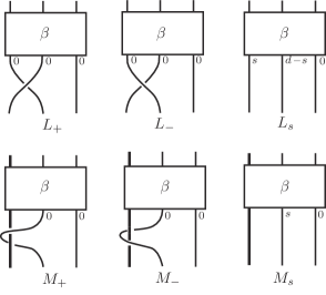
Figure 3. The elements $L_{+}$, $L{-}$, $L_{s}$, $M_{+}$, $M_{-}$ and $M_{s}$ in open braid form.

Proof.

Both skein relations are easily derived from the quadratic relations of ${\rm Y}_{d,n}^{\mathtt{B}}(\mathsf{u},\mathsf{v})$. Denote now $\Lambda_{S}:=\frac{1-\lambda_{S}}{\sqrt{\lambda_{S}}(\mathsf{u}-\mathsf{u}^{-1}){\rm E}_{S}}$. For the first skein relation we have:

$${\mathcal{X}}_{S}^{\mathtt{B}}(\widehat{\beta g_{i}^{-1}}) =\Lambda_{S}^{n-1}\left(\sqrt{\lambda_{S}}\right)^{\varepsilon(\beta-1)}{\rm Tr}(\beta g_{i}^{-1})$$

$$=\Lambda_{S}^{n-1}\left(\sqrt{\lambda_{S}}\right)^{\varepsilon(\beta-1)}{\rm Tr}(\beta g_{i})+(\mathsf{u}-\mathsf{u}^{-1})\Lambda_{S}^{n-1}\left(\sqrt{\lambda_{S}}\right)^{\varepsilon(\beta-1)}{\rm Tr}(\beta e_{i})$$

$$=\frac{1}{\lambda_{S}}\Lambda_{S}^{n-1}\left(\sqrt{\lambda_{S}}\right)^{\varepsilon(\beta+1)}{\rm Tr}(\beta g_{i})+\frac{(\mathsf{u}-\mathsf{u}^{-1})}{\sqrt{\lambda_{S}}}\Lambda_{S}^{n-1}\left(\sqrt{\lambda_{S}}\right)^{\varepsilon(\beta)}{\rm Tr}(\beta e_{i})$$

$$=\frac{1}{\lambda_{S}}{\mathcal{X}}_{S}^{\mathtt{B}}(\widehat{\beta g_{i}})+\frac{(\mathsf{u}-\mathsf{u}^{-1})}{d\sqrt{\lambda}}\sum_{s=0}^{d-1}{\mathcal{X}}_{S}^{\mathtt{B}}(\beta t_{i}^{s}t_{i+1}^{d-s})$$

which leads to

$$\frac{1}{\sqrt{\lambda_{S}}}{\mathcal{X}}_{S}^{\mathtt{B}}(L_{+})-\sqrt{\lambda_{S}}{\mathcal{X}}_{S}^{\mathtt{B}}(L_{-})=\frac{\mathsf{u}-\mathsf{u}^{-1}}{d}\sum_{s=0}^{d-1}{\mathcal{X}}_{S}^{\mathtt{B}}(L_{s}).$$

In an analogous way, we prove the second skein relation.

$${\mathcal{X}}_{S}^{\mathtt{B}}(\widehat{\beta b_{i}^{-1}}) =\Lambda_{S}^{n-1}\left(\sqrt{\lambda_{S}}\right)^{\varepsilon(\beta)}{\rm Tr}(\beta b_{i}^{-1})$$

$$=\Lambda_{S}^{n-1}\left(\sqrt{\lambda_{S}}\right)^{\varepsilon(\beta)}{\rm Tr}(\beta b_{i})+(\mathsf{v}-\mathsf{v}^{-1})\Lambda_{S}^{n-1}\left(\sqrt{\lambda_{S}}\right)^{\varepsilon(\beta)}{\rm Tr}(\beta f_{i})$$

$$=\Lambda_{S}^{n-1}\left(\sqrt{\lambda_{S}}\right)^{\varepsilon(\beta)}{\rm Tr}(\beta b_{i})+(\mathsf{v}-\mathsf{v}^{-1})\Lambda_{S}^{n-1}\left(\sqrt{\lambda_{S}}\right)^{\varepsilon(\beta)}{\rm Tr}(\beta f_{i})$$

$$={\mathcal{X}}_{S}^{\mathtt{B}}(\widehat{\beta b_{i}})+\frac{(\mathsf{v}-\mathsf{v}^{-1})}{d}\sum_{s=0}^{d-1}{\mathcal{X}}_{S}^{\mathtt{B}}(\beta t_{i}^{s})$$

which is equivalent to:

$${\mathcal{X}}_{S}^{\mathtt{B}}(M_{+})-{\mathcal{X}}_{S}^{\mathtt{B}}(M_{-})=\frac{\mathsf{v}-\mathsf{v}^{-1}}{d}\sum_{s=0}^{d-1}{\mathcal{X}}_{S}^{\mathtt{B}}(M_{s}),$$

∎

The link invariants on the level of ${\rm FTL}^{\mathtt{B}}_{d,n}(\mathsf{u},\mathsf{v})$ will be specializations of the invariants ${\mathcal{X}}_{S}^{\mathtt{B}}(\lambda,\mathsf{u},\mathsf{v})$ for specific values of the trace parameters $x_{i}$, $y_{j}$ and $z$. Theorem 5 provides the conditions so that these new invariants are well-defined. Of course, not all values for $x_{i}$, $y_{j}$ and $z$ furnish topologically interesting link invariants and so we shall use Corollary 1 to filter out such values.

In this context, we discard the cases $1(i)$, $2(i)$ and $2(ii)$ of Corollary 1. The reason behind this is that if we specialize the trace parameters in the expression of ${\mathcal{X}}_{S}^{\mathtt{B}}$ to any of the cases mentioned just above, we will obtain an invariant that fails to distinguish basic pairs of links. In more detail, for $d=1$ we have that $x_{k}=1$ and so the parameters $z$ and $y_{k}$ correspond to values that were discarded in the classical case. From the surviving values of Corollary 1, we deduce that the rescaling factor $\lambda_{S}=\mathsf{u}^{4}$ and so we have:

Definition 5.

Let ${\rm X}=({\rm x}_{1},\ldots,{\rm x}_{d-1})$ a solution of the ${\rm E}$-system, $S\subset C_{d}$ that parametrizes said solution. Let also the trace parameters $y_{k}$ to be as in case 1(ii) of Corollary 1 and let $z=-\frac{1}{\mathsf{u}(\mathsf{u}^{2}+1)|S|}$. Then, the following map is an invariant of framed links inside the solid torus:

$$\rho_{S}^{\mathtt{B}}(\mathsf{u},\mathsf{v})(\widehat{\alpha}):=\left(-\frac{1+\mathsf{u}^{2}}{{\rm E}_{S}\mathsf{u}}\right)^{n-1}\mathsf{u}^{2\varepsilon(\alpha)}{\rm Tr}(\bar{\pi}(\alpha))={\mathcal{X}}_{S}^{\mathtt{B}}(\mathsf{u}^{4},\mathsf{u},\mathsf{v}),$$

where ${\rm E_{S}}$, $\varepsilon(\alpha)$ and $\bar{\pi}:\mathcal{F}^{\mathtt{B}}_{d,n}\rightarrow{\rm FTL}_{d,n}^{\mathtt{B}}(\mathsf{u},\mathsf{v})$ that sends $\sigma_{i}\mapsto g_{i}$ and $t_{i}\mapsto t_{i}$.

Since the invariants $\rho_{S}^{\mathtt{B}}$ are specializations of ${\mathcal{X}}_{S}^{\mathtt{B}}$, they should satisfy also a specialized version of the skein relations of Proposition 5. Indeed, by substituting $\lambda_{S}=\mathsf{u}^{4}$ in Proposition 5 we obtain:

Proposition 6.

The invariants $\rho_{S}^{\mathtt{B}}(\mathsf{u},\mathsf{v})$ satisfy the following two skein relations:

$$\mathsf{u}^{-2}\rho_{S}^{\mathtt{B}}(L_{+})-\mathsf{u}^{2}\rho_{S}^{\mathtt{B}}(L_{-})=\frac{\mathsf{u}-\mathsf{u}^{-1}}{d}\sum_{s=0}^{d-1}\rho_{S}^{\mathtt{B}}(L_{s}),$$

where $L_{+}=\widehat{\beta g_{i}}$, $L_{-}=\widehat{\beta g_{i}^{-1}}$,$L_{s}=\widehat{\beta t_{i}^{s}t_{i+1}^{d-s}}$, $\beta=\pi(\alpha)$, $\alpha\in\widehat{W}_{n}$ and $\pi:\widehat{W}_{n}\rightarrow{\rm Y}_{d,n}^{\mathtt{B}}$.

$$\rho_{S}^{\mathtt{B}}(M_{+})-\rho_{S}^{\mathtt{B}}(M_{-})=\frac{\mathsf{v}-\mathsf{v}^{-1}}{d}\sum_{s=0}^{d-1}\rho_{S}^{\mathtt{B}}(M_{s}),$$

where $M_{+}=\widehat{\beta b_{i}}$, $M_{-}=\widehat{\beta b_{i}^{-1}}$ and $M_{s}=\widehat{\beta t_{i}^{s}}$ and $\beta\in\widehat{W}_{n}$.

Remark 4.

Notice that for $d=1$, $\rho_{S}^{\mathtt{B}}(\mathsf{u},\mathsf{v})$ coincides with the case of classical links in (3.5). Moreover, for $d=1$ the skein relations of Proposition 5 coincide with the skein relations (3.6) and (3.7).

5.2. Classical link invariants in the solid torus

Restricting $\pi$ to classical braids, seen as framed braids with all framings equal zero, one obtains from $\rho_{S}^{\mathtt{B}}(\mathsf{u},\mathsf{v})$ an invariant for classical links, which is denoted by $\eta:=\eta_{S}^{\mathtt{B}}(\mathsf{u},\mathsf{v})$. The invariant $\eta$ satisfies the same skein relations as $\rho_{S}^{\mathtt{B}}(\mathsf{u},\mathsf{v})$. Notice that the algebra ${\rm FTL}_{d,n}(u)$ can be seen as a subalgerba of ${\rm FTL}_{d,n}^{\mathtt{B}}$. Indeed, the image of the map

$$\phi:{\rm FTL}_{d,n}(u)\longrightarrow{\rm FTL}_{d,n}^{\mathtt{B}},$$

that sends $g_{i}\mapsto g_{i}$ and $t_{i}\mapsto t_{i}$, is isomorphic to ${\rm FTL}_{d,n}(u)$. Therefore, the trace ${\rm Tr}$, when restricted to $\phi({\rm FTL}_{d,n}(u)$), coincides with the trace $tr$ of ${\rm FTL}_{d,n}(u)$.

A link $L$ inside the solid torus $T$ is called affine if it lies inside a 3-ball $B\subset T$. Any link in $S^{3}$ can be seen as an embedded affine link in the solid torus. From the above, we can deduce that the invariant $\eta$ contains the invariant $\theta_{d}$ and so it distinguishes at least the same number of non-isotopic links as $\theta_{d}$.

More precisely, the invariant $\theta_{d}$ distinguishes six pairs of non-isotopic links that are not distinguished by the Jones polynomial [15]. Moreover, $\theta_{d}$ generalizes to the two-variable link invariant $\theta(q,E)$ that is topologically equivalent to the Jones polynomial on knots but stronger than the Jones polynomial on links [15, Theorem 5]. Consequently, it is different than the Homflypt and the Kauffman polynomials. It has been shown as well [15, 3] that $\theta(q,E)$ distinguishes two links from the Eliahou-Kaufmann-Thistlethwaite infinite family of links [7] that have the same Jones polynomial as the $k$-component unknot. By specializing $E=1/d$, one can confirm that $\theta_{d}$ also distinguishes these two links. Figure 4 collects all pairs of affine links that are known to be distinguished by the invariant $\eta$.

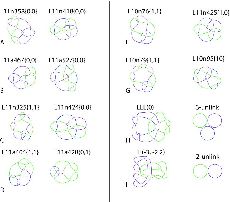
Figure 4. Pairs of affine links that are distinguished by the invariant $\eta$ and not by the Jones polynomial. Note that pairs H and I and unoriented. Pairs A-G follow the Thistelthwaite notation [2]. Pairs H and I follow the Eliahou-Kauffman-Thistelthwaite notation [7].

5.3. Future work

The observation that the invariant $\eta$ contains $\theta_{d}$ suggests that $\eta$ is stronger than the Jones polynomial in the solid torus, at least on affine links, and that it is different than the Homflypt polynomial in the solid torus. Consider the map $\delta:\mathbb{K}\widetilde{W}_{n}\longrightarrow{\rm Y}_{d,n}^{\mathtt{B}}$ that sends $\sigma_{i}\mapsto g_{i}$. In analogy to [5] we have that $\delta(\mathbb{K}\widetilde{W}_{n})$ is isotopic to ${\rm Y}^{\mathtt{B}}_{(br)}$, the subalgebra of ${\rm Y}_{d,n}^{\mathtt{B}}$ generated only by the braiding and the looping generators. Note that in ${\rm Y}^{\mathtt{B}}_{(br)}$ the generators $t_{i}$ appear only in the idempotents $e_{i}$ and $f_{j}$ and only after the application of one of the quadratic relations. However, they still have an impact on the skein relation, as they introduce terms with summations (recall Proposition 6). Unfortunately, this makes difficult to compare $\eta$ to other invariants in the solid torus on non-affine links.

In order to overcome this obstacle, we follow the method of [5, 15]. Let $\mathcal{E}_{n}^{\mathtt{B}}$ be the algebra of braids and ties of type $\mathtt{B}$ [9] that is generated by the braiding generators $T_{i}$ ($i=1\ldots n-1$) the looping generator $B_{1}$, and the idempotents $E_{i}$ ($i=1\ldots n-1$) and $F_{j}$ ($j=1,\ldots n$). For $d>n+1$, the map $\mathcal{E}_{n}^{\mathtt{B}}\longrightarrow{\rm Y}_{d,n}^{\mathtt{B}}$ is an embedding [9], which, again in analogy to [5], implies that $\mathcal{E}_{n}^{\mathtt{B}}\cong{\rm Y}^{\mathtt{B}}_{(br)}$.

This means that in the context of classical links in the solid torus, seen as closures of framed braids in the solid torus with all framings equal zero, we can work directly with $\mathcal{E}_{n}^{\mathtt{B}}$. The advantage is that the framing generators are not involved in the definition of $\mathcal{E}_{n}^{\mathtt{B}}$, which simplifies the corresponding skein relations. For the purpose of our comparison we aim to generalize the invariant $\eta$ to a three-variable invariant. One could achieve this by defining the partition Temperley-Lieb algebra of type $\mathtt{B}$, ${\rm PTL}_{n}^{\mathtt{B}}$, as an appropriate quotient of $\mathcal{E}_{n}^{\mathtt{B}}$ and determine the necessary and sufficient conditions so that the trace ${\rm\mathbf{tr}}_{n}$ of $\mathcal{E}_{n}^{\mathtt{B}}$ passes to ${\rm PTL}_{n}^{\mathtt{B}}$. Under these conditions, we will obtain the desired generalized invariant. This is a work in progress and it will be the subject of a sequel paper.

References

- [1] J. S. Birman and H. Wenzl, Braids, link polynomials and a new algebra, Transactions of the American Mathematical Society, 313 (1989), pp. 249–273.
- [2] J. C. Cha and C. Livingston, Linkinfo: Table of knot invariants. http://www.indiana.edu/ linkinfo, 12 Nov 2019.
- [3] M. Chlouveraki, From the Framisation of the Temperley-Lieb algebra to the Jones polynomial: an algebraic approach, in Knots, Low-Dimensional Topology and Applications, Springer PROMS series, C. C. Adams, C. M. Gordon, V. F. Jones, L. H. Kauffman, S. Lambropoulou, K. C. Millett, J. H. Przytycki, R. Ricca, and R. Sazdanovic, eds., Springer.
- [4] M. Chlouveraki and L. P. D’Andecy, Markov trace on affine and cyclotomic Yokonuma-Hecke algebras, Int. Math. Res. Notices, 2016 (2016), pp. 4167–4228.
- [5] M. Chlouveraki, J. Juyumaya, K. Karvounis, and S. Lambropoulou, Identifying the invariants for classical knots and links from the Yokonuma-Hecke algebras, submitted for publication. See also arXiv:1505.06666, (2015).
- [6] M. Chlouveraki and G. Pouchin, Representation theory and an isomorphism theorem for the Framisation of the Temperley-Lieb algebra, arXiv:1503.03396v2, (2015).
- [7] S. Eliahou and M. T. L. H. Kauffman, Infinite families of links with trivial jones polynomial, Topology, 42 (2003), pp. 155–169.
- [8] C. K. Fan and R. M. Green, Monomials and temperley-lieb algebras, Journal of algebra., 190 (1997), pp. 498–517.
- [9] M. Flores, A braid and ties algebra of type , Journal of Pure and Applied Algebra, 224 (2020), pp. 1–32.
- [10] M. Flores, J. Juyumaya, and S. Lambropoulou, A framization of the Hecke algebra of type , in press J. Pure Appl. Algebr. https://doi.org/10.1016/j.jpaa.2017.05.006, (2016).
- [11] M. Geck and S. Lambropoulou, Markov traces and knot invariants related to Iwahori-Hecke algebras of type B, J. Reine Angew. Math., 482 (1997), p. 191–213.
- [12] D. Goundaroulis, Framization of the Temperley-Lieb algebra and related link invariants, PhD thesis, Department of Mathematics, National Technical University of Athens, 1 2014.
- [13] D. Goundaroulis, J. Juyumaya, A. Kontogeorgis, and S. Lambropoulou, The Yokonuma-Temperley-Lieb Algebra, Banach Center Pub., 103 (2014), pp. 73–95.
- [14] , Framization of the Temperley-Lieb Algebra, Math. Res. Lett., 24 (2017), pp. 299–345.
- [15] D. Goundaroulis and S. Lambropoulou, A new two-variable generalization of the Jones polynomial. J. Knot Theory Ramif. Online ready. https://doi.org/10.1142/S0218216519400054, 2019.
- [16] R. M. Green and J. Losonczy, Canonical bases for hecke algebra quotients, Math. Res. Lett., 6 (1999), pp. 213–222.
- [17] J. Humphreys, Reflection Groups and Coxeter Groups, Cambridge University Press, 1990.
- [18] V. Jones, Index for subfactors, Inventiones Mathematicae, 72 (1983), pp. 1–25.
- [19] , Hecke algebra representations of braid groups and link polynomials, Annals of Mathematics, 126 (1987), pp. 335–388.
- [20] J. Juyumaya, Sur les nouveaux générateurs de l’algèbre de Hecke , J. Algebra, 204 (1998), pp. 40–68.
- [21] , Markov trace on the Yokonuma-Hecke algebra, J. Knot Theory and Its Ramifications, 13 (2004), pp. 25–39.
- [22] J. Juyumaya and S. Lambropoulou, -adic framed braids, Topology and its Applications, 154 (2007), pp. 1804–1826.
- [23] , An adelic extension of the jones polynomial, in The mathematics of knots, M. Banagl and D. Vogel, eds., Contributions in the Mathematical and Computational Sciences, Vol. 1, Springer, 2009, pp. 825–840.
- [24] , An invariant for singular knots, J. Knot Theory and Its Ramifications, 18 (2009), pp. 825–840.
- [25] , Modular framization of the BMW algebra. arXiv:1007.0092v1 [math.GT], 2013.
- [26] , -adic framed braids II, Advances in Mathematics, 234 (2013), pp. 149–191.
- [27] S. Lambropoulou, Solid torus links and Hecke algebras of B-type, in Proceedings of the Conference on Quantum Topology, D. N. Yetter ed., World Scientific Press, 1994.
- [28] A. Mathas, Iwahori–Hecke algebras and Schur algebras of the Symmetric gruop, AMS, 1999.
- [29] J. Murakami, The kauffman polynomial of links and representation theory, New Developments In The Theory Of Knots. Series: Advanced Series in Mathematical Physics, ISBN: 978-981-02-0162-3. WORLD SCIENTIFIC, Edited by Toshitake Kohno, vol. 11, pp. 480-493, 11 (1990), pp. 480–493.
- [30] H. Temperley and E. H. Lieb, Relations between the ‘percolation’ and ‘couloring’ problem and other graph-theoretical problem associated with regular planar lattice: some exact results for the ‘percolations problems’, Proc. Roy. Soc. London Ser. A, 322 (1971), pp. 251–280.
- [31] A. Terras, Fourier Analysis of Finite Groups and Applications, London Math. Soc. student text, 1999.
- [32] T. Yokonuma, Sur la structure des anneux de Hecke d’un group de Chevalley fin, C.R. Acad. Sc. Paris, 264 (1967), pp. 344–347.