The 2014-2017 outburst of the young star ASASSN-13db:

Abstract

Context. Accretion outbursts are key elements in star formation. ASASSN-13db is a M5-type star with a protoplanetary disk, the lowest-mass star known to experience accretion outbursts. Since its discovery in 2013, it has experienced two outbursts, the second of which started in November 2014 and lasted until February 2017.

Aims. We explore the photometric and spectroscopic behavior of ASASSN-13db during the 2014-2017 outburst.

Methods. We use high- and low-resolution spectroscopy and time-resolved photometry from the ASAS-SN survey, the LCOGT and the Beacon Observatory to study the lightcurve of ASASSN-13db and the dynamical and physical properties of the accretion flow.

Results. The 2014-2017 outburst lasted for nearly 800 days. A 4.15d period in the light curve likely corresponds to rotational modulation of a star with hot spot(s). The spectra show multiple emission lines with variable inverse P-Cygni profiles and a highly variable blue-shifted absorption below the continuum. Line ratios from metallic emission lines (Fe I/Fe II, Ti I/Ti II) suggest temperatures of $\sim$5800-6000 K in the accretion flow.

Conclusions. Photometrically and spectroscopically, the 2014-2017 event displays an intermediate behavior between EXors and FUors. The accretion rate (Ṁ=1-3$\times$10^-7M_⊙/yr), about two orders of magnitude higher than the accretion rate in quiescence, is not significantly different from the accretion rate observed in 2013. The absorption features in the spectra suggest that the system is viewed at a high angle and drives a powerful, non-axisymmetric wind, maybe related to magnetic reconnection. The properties of ASASSN-13db suggest that temperatures lower than those for solar-type stars are needed for modeling accretion in very-low-mass systems. Finally, the rotational modulation during the outburst reveals that accretion-related structures settle after the beginning of the outburst and can be relatively stable and long-lived. Our work also demonstrates the power of time-resolved photometry and spectroscopy to explore the properties of variable and outbursting stars.

1 Introduction

Variability is one of the defining characteristics of young T Tauri stars (TTS; Joy, 1945). Together with rotational modulation due to stellar spots and extinction by circumstellar material, changes in the accretion rate are one of the reasons for their variability (Herbst et al., 1994). Although most TTS appear to undergo only mild accretion variations on timescales of days to years (e.g., Sicilia-Aguilar et al., 2010; Costigan et al., 2014), the accretion rates of some TTS can change by several orders of magnitude on timescales of weeks to decades. Such eruptive variables are classified as FUors and EXors, named after their respective prototypes FU Orionis (Herbig, 1977, 1989; Hartmann & Kenyon, 1996) and EX Lupi (Herbig et al., 2001; Herbig, 2008). Accretion outbursts play an important role in the formation of stars, and may be the key to solving the protostellar luminosity problem (Kenyon & Hartmann, 1995; Dunham & Vorobyov, 2012) and the formation of cometary material in the Solar System (Ábrahám et al., 2009). The distinction between the two classes lies in the magnitude of the outburst, the increase of accretion, the shape of the light curve, and the spectral features observed during outburst. The characteristics of individual objects do not always fully coincide with one of the classes (Herczeg et al., 2016), and some authors have suggested that the two classes (or at least, a subset of them) are part of a continuous spectrum of outbursting stars (Contreras Peña et al., 2014, 2017).

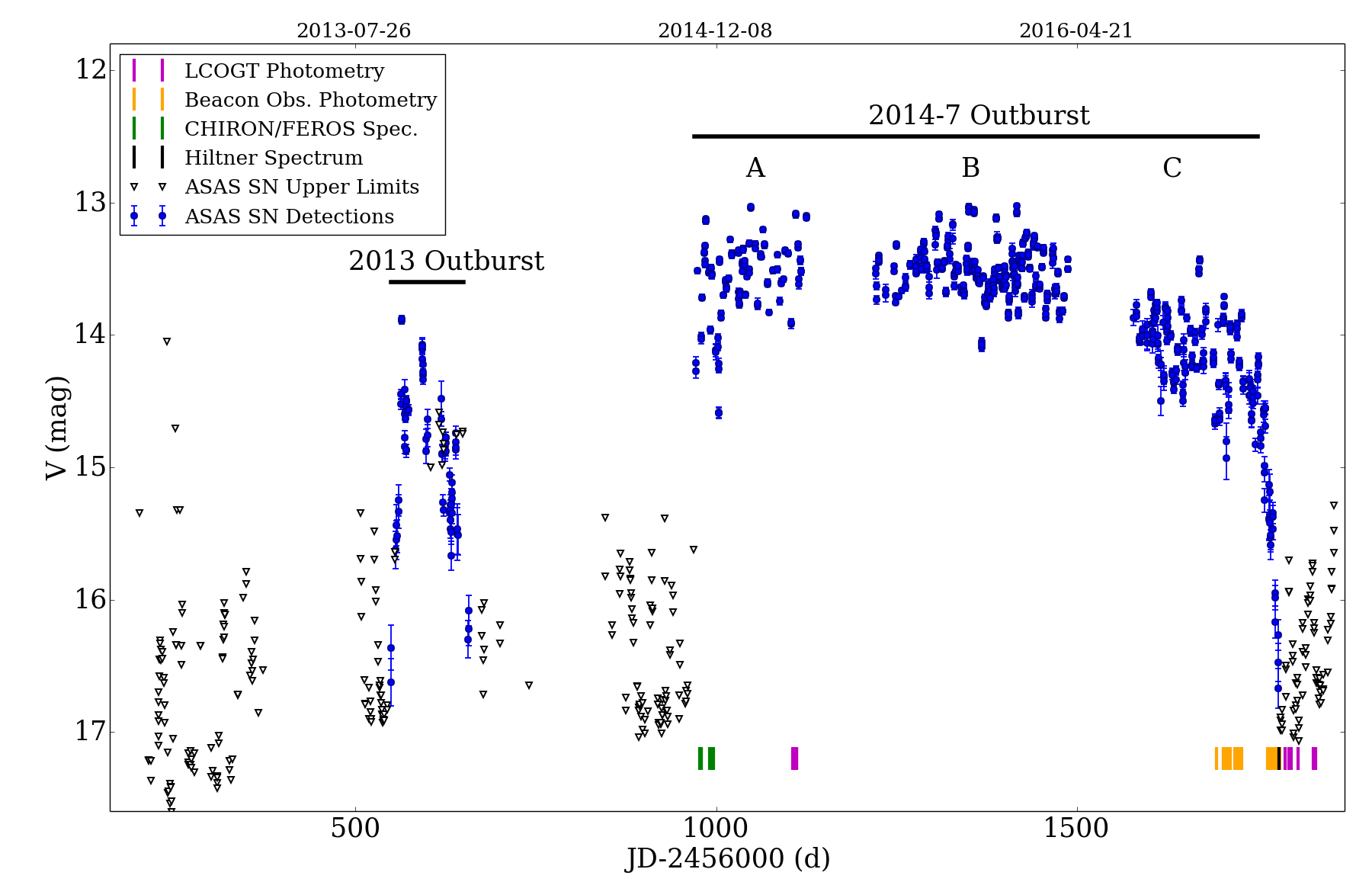
Figure 1: V-band ASASSN-13db light curve from ASAS-SN. Detections and non-detections are shown as dots (with errors) and inverted triangles, respectively. The dates at which we acquired the rest of the observations and the periods of the two known outbursts are also marked.

The low-mass star SDSS J05101100-0328262, also known as SDSSJ0510 and ASASSN-13db (Holoien et al., 2014), is a variable star that was identified by the All Sky Automated Survey for SuperNovae (ASAS-SN) after a four-magnitude brightness increase in September 2013 (Shappee et al., 2014; Holoien et al., 2014). Spectroscopic observations during the 2013 outburst revealed a rich emission line spectrum, leading to its classification as an EXor variable (Holoien et al., 2014). The spectrum contained hundreds of metallic emission lines, so that the object was dubbed ”the EX Lupi twin”, entering the category as one of the most impressive EXor variables considering its photometric variability and spectral features (Holoien et al., 2014). Being a very red star with substantial IR emission consistent with a protoplanetary disk (Holoien et al., 2014), it is likely a member of the young star-forming regions within the L1615/L1616 Orion cometary clouds. The regions are part of the open cluster NGC 1981 to the north of the Orion Nebula Cluster (ONC). ASASSN-13db would have an approximate age of 1-3 Myr based on other stars in the same region (Gandolfi et al., 2008). Further observations during quiescence in January 2014 confirmed that ASASSN-13db is a young, accreting TTS M5-type star, which also makes it the lowest-mass EXor identified to date (Holoien et al., 2014). After a brief period of quiescence during 2014, ASASSN-13db went into outburst again in November 2014 (ASAS SN CV Patrol; Davis et al., 2015).

In this paper we present the photometric and spectroscopic followup of ASASSN-13db during the 2014-2017 outburst. In Section 2 we describe the observations and the data reduction. In Sections 3 and 4 we analyze the light curve and the spectral emission and absorption features observed during the outburst. In Section 5 we discuss the nature of the outburst. Finally, in Section 6 we summarize our results.

2 Observations and data reduction

2.1 Photometry

ASASSN-13db was tracked during the outburst and return to quiescence by the All Sky Automated Survey for SuperNovae (ASAS-SN; Shappee et al., 2014), the Las Cumbres Observatory Global Telescope Network (LCOGT; Brown et al., 2013), the Beacon Observatory telescope in Kent, and some amateur astronomers.

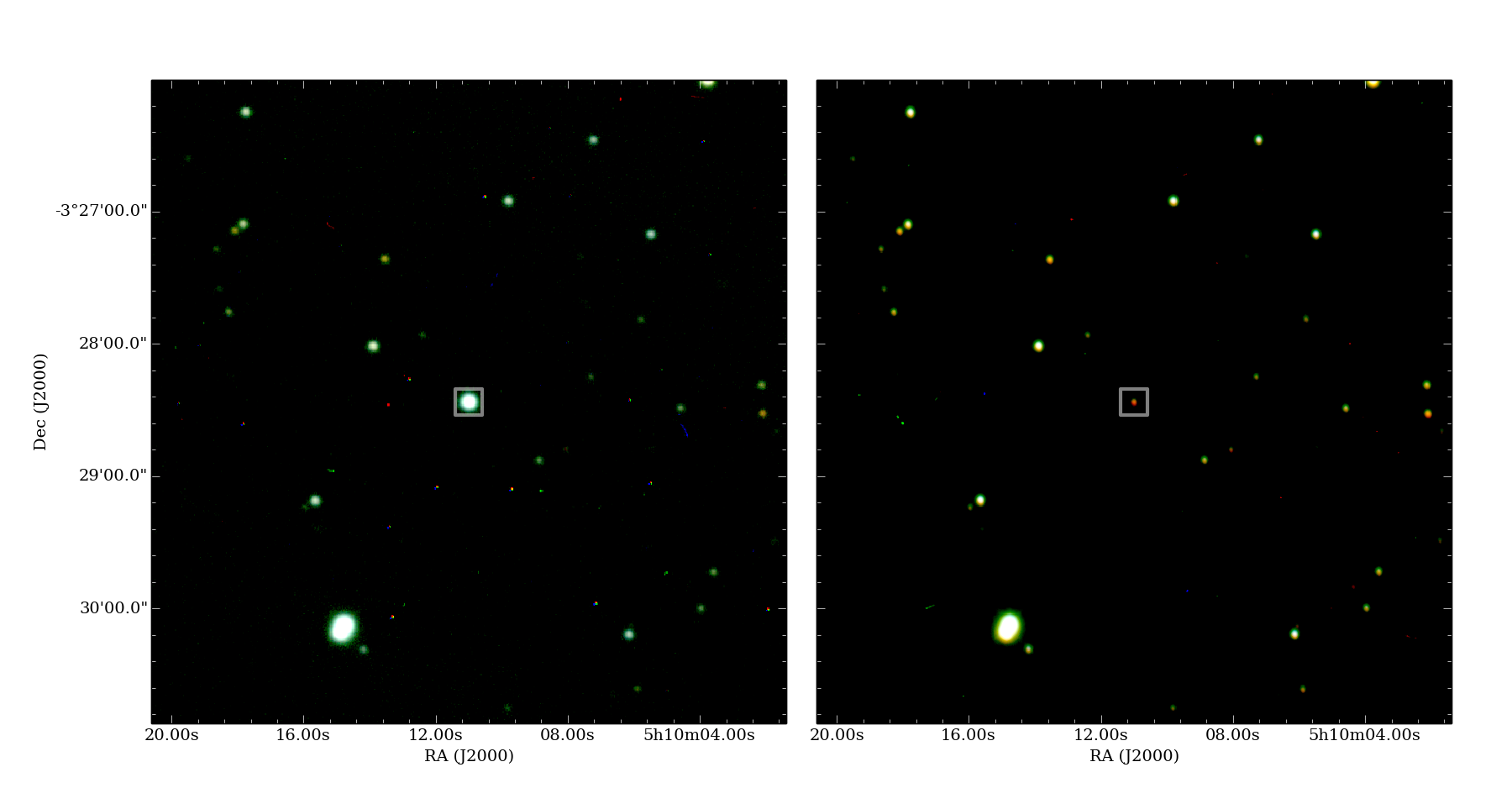
Figure 2: LCOGT RGB (R=$i^{\prime}$, G=$r^{\prime}$, B=$g^{\prime}$) images of ASASSN-13db obtained during the outburst (left, JD=2457110.243) and post-outburst phases (right, JD=2457805.288). ASASSN-13db is marked with a square. We note the change in brightness and color.

The most complete photometric followup of the object since its discovery in 2013 is the V band light curve provided by ASAS-SN. The ASAS-SN data were reduced using the standard ASAS-SN pipeline (Shappee et al. in prep.). We performed aperture photometry at the location of ASASSN-13db using the IRAF apphot package and calibrated the results using the AAVSO Photometric All Sky Survey (Henden & Munari, 2014). Photometry and 5 $\sigma$ upper limits are reported in Table 1. The star is too dim for ASAS-SN during quiescence. Two well-defined outbursts are seen in the data (see Figure 1). The first one, ending in January 2014, corresponds to a typical EXor outburst (Holoien et al., 2014). The object increased in brightness by at least three magnitudes and returned to quiescence within a few months. The second outburst started in November 2014 (approximately, on Julian Date [JD] 2456560) with a rapid increase in brightness of over four magnitudes with respect to the minimum in 2013/4, and ended in February 2017. Except for two $\sim$3-month gaps due to object visibility, we have continuous coverage. From now on, we refer to the three parts of the outburst, separated by observation gaps, as ”A”, ”B”, and ”C” (see Figure 1). The 2014-2017 outburst spans $\sim$770 days, or about 2 years and 1.5 months. It is very unlikely that the star returned to quiescence during the times when no observations are available, taking into account the timescale of the 2013 outburst and the length of the final dimming. We thus consider that the star has been in continuous outburst from November 2014 until February 2017.

Table 1: ASAS-SN photometry.

JD	V
(d)	(mag)
2456539.06603	$>$16.93
2456540.05305	$>$16.86
2456540.05443	$>$16.94
2456544.04266	$>$16.80
2456544.04403	$>$16.83
2456550.01831	16.37$\pm$0.17
2456550.01967	16.64$\pm$0.18
2456555.00243	$>$15.64
2456555.00386	$>$15.71
2456556.04073	15.62$\pm$0.14
2456556.04209	15.79$\pm$0.22
2456557.02096	15.56$\pm$0.15
2456557.02233	15.44$\pm$0.16
2456558.04729	15.49$\pm$0.12
2456560.00528	15.38$\pm$0.13
2456560.00666	15.25$\pm$0.12
2456562.98509	14.53$\pm$0.04
2456562.98645	14.45$\pm$0.04
2456564.13425	13.91$\pm$0.02
2456564.13562	13.88$\pm$0.02

The multi-band photometric data from LCOGT were taken during the outburst (March 24-29, 2015) and post-outburst/quiescence phases (February 2, 2017 - March 17, 2017), using the $u^{\prime}$, $g^{\prime}$, $r^{\prime}$ and $i^{\prime}$ Sloan filters. During the outburst, we obtained 100s of exposure per band. During the post-outburst phase, we obtained a short (60s) and a long (300s) exposure for $g^{\prime}$, and long (300s) exposures for $r^{\prime}$ and $i^{\prime}$. The object was too faint to be detected in $u^{\prime}$ band during the post-outburst phase. Figure 2 captures the impressive change in brightness and color between the outburst and quiescence phases, as seen by LCOGT.

The data were reduced (debiased, flat fielded, and aligned) using the standard LCOGT pipeline. We then performed aperture photometry using IRAF daofind and apphot packages. Finally, we extracted the relative instrumental magnitudes by calibrating all the observations against a LCOGT reference image (the best-quality data) and Sloan Digital Sky Survey (Gunn et al., 2006; Doi et al., 2010); data available via SkyServer. A total of 492, 738, and 640 stars were used to calibrate the $g^{\prime}$, $r^{\prime}$, and $i^{\prime}$ filters, respectively. We also attempted to calibrate the $u^{\prime}$ band using the data from the outburst taken on JD 2457110.287, but due to having only five matches, of which at least two appeared to be variable, the calibration has a large error and has to be regarded with extreme care. The errors in the flux calibration of the LCOGT data (5% for $g^{\prime}$, 3% for $r^{\prime}$, and 4% for $i^{\prime}$, about 60% for $u^{\prime}$) have not been added to the total and thus do not appear in the table or plots. Table 2 contains the final magnitudes from the LCOGT, and the resulting light curve is displayed in Figure 3.

Table 2: Final calibrated photometry from the LCOGT data.

JDini	JD${}_{u^{\prime}}$	$u^{\prime}$	JD${}_{g^{\prime}}$	$g^{\prime}$	JD${}_{r^{\prime}}$	$r^{\prime}$	JD${}_{i^{\prime}}$	$i^{\prime}$
		(mag)		(mag)		(mag)		(mag)
Outburst
2457106.26	—	—	2457106.258	13.97$\pm$0.01	2457106.263	13.26$\pm$0.01	2457106.261	12.91$\pm$0.01
2457106.88	—	—	2457106.878	14.02$\pm$0.02	2457106.882	13.28$\pm$0.02	2457106.880	12.97$\pm$0.02
2457106.89	—	—	2457106.888	14.02$\pm$0.02	2457106.892	13.30$\pm$0.02	2457106.890	12.97$\pm$0.02
2457107.23	—	—	2457107.233	14.08$\pm$0.03	2457107.238	13.37$\pm$0.04	2457107.236	13.08$\pm$0.03
2457107.29	—	—	2457107.285	13.78$\pm$0.04	2457107.289	13.47$\pm$0.04	2457107.287	13.03$\pm$0.04
2457107.90	2457107.902	19.17$\pm$0.48u	22457107.897	13.90$\pm$0.02	2457107.900	13.18$\pm$0.01	2457107.898	12.85$\pm$0.02
2457108.23	2457108.238	18.70$\pm$0.06u	2457108.232	13.63$\pm$0.02	2457108.236	13.15$\pm$0.01	2457108.234	12.88$\pm$0.02
2457109.23	—	—	2457109.231	13.55$\pm$0.02	2457109.235	12.86$\pm$0.01	2457109.233	12.62$\pm$0.02
2457110.23	—	—	2457110.231	13.54$\pm$0.03	—	—	2457110.23	12.78$\pm$ 0.04
2457110.24	—	—	2457110.243	13.47$\pm$0.02	2457110.247	12.94$\pm$0.01	2457110.245	12.71$\pm$0.02
2457110.27	—	—	2457110.273	13.51$\pm$0.02	2457110.277	12.97$\pm$0.04	2457110.275	12.76$\pm$0.03
2457110.29	2457110.295	18.39$\pm$0.04u	2457110.287	13.48$\pm$0.01	2457110.292	12.95$\pm$0.01	2457110.289	12.72$\pm$0.01
2457111.23	—	—	—	—	2457111.235	13.10$\pm$0.02	2457111.233	12.86$\pm$0.02
2457111.25	—	—	2457111.253	13.79$\pm$0.02	—	—	2457111.259	12.97$\pm$0.02
2457111.27	2457111.274	18.75$\pm$0.06u	2457111.268	13.83$\pm$0.02	2457111.272	13.20$\pm$0.02	2457111.270	12.91$\pm$0.02
2457702.50a	—	—	—	—	2457702.497	15.26$\pm$0.07	2457702.553	16.09$\pm$0.06
Post-outburst
2457787.30	—	—	2457787.304	18.30$\pm$0.03	2457787.328	17.39$\pm$0.05	2457787.316	16.41$\pm$0.02
2457787.31	—	—	2457787.308	18.20$\pm$0.04	2457787.332	17.45$\pm$0.05	2457787.320	16.41$\pm$0.02
2457787.31	—	—	2457787.312	18.19$\pm$0.05	2457787.336	17.32$\pm$0.05	2457787.324	16.41$\pm$0.02
2457793.33	—	—	2457793.328	18.28$\pm$0.09	—	—	—	—
2457793.33	—	—	2457793.330	18.22$\pm$0.04	2457793.354	17.53$\pm$0.04	2457793.342	16.46$\pm$0.02
2457793.33	—	—	2457793.334	18.28$\pm$0.04	2457793.358	17.46$\pm$0.04	2457793.346	16.44$\pm$0.02
2457793.34	—	—	2457793.338	18.23$\pm$0.04	2457793.362	17.51$\pm$0.04	2457793.350	16.36$\pm$0.02
2457796.34	—	—	2457796.344	18.36$\pm$0.08	—	—	—	—
2457796.35	—	—	2457796.345	18.27$\pm$0.04	2457796.369	17.54$\pm$0.04	2457796.357	16.45$\pm$0.02
2457796.35	—	—	2457796.349	18.31$\pm$0.04	2457796.373	17.52$\pm$0.04	2457796.361	16.46$\pm$0.02
2457796.35	—	—	2457796.353	18.32$\pm$0.04	2457796.377	17.57$\pm$0.04	2457796.365	16.44$\pm$0.02
2457798.33a	—	—	—	—	2457798.338	17.16$\pm$0.08	2457798.330	16.44$\pm$0.08
2457805.29	—	—	2457805.287	18.47$\pm$0.04	—	—	—	—
2457805.29	—	—	2457805.288	18.49$\pm$0.01	2457805.312	17.80$\pm$0.01	2457805.300	16.52$\pm$0.01
2457805.29	—	—	2457805.292	18.49$\pm$0.02	2457805.316	17.79$\pm$0.02	2457805.304	16.53$\pm$0.01
2457805.30	—	—	2457805.296	18.48$\pm$0.02	2457805.320	17.81$\pm$0.01	2457805.308	16.53$\pm$0.01
2457805.34	—	—	2457805.338	18.60$\pm$0.06	—	—	—	—
2457805.34	—	—	2457805.340	18.66$\pm$0.03	2457805.364	17.85$\pm$0.03	2457805.352	16.58$\pm$0.02
2457805.34	—	—	2457805.344	18.69$\pm$0.03	2457805.368	17.82$\pm$0.03	2457805.356	16.56$\pm$0.02
2457805.35	—	—	2457805.348	18.76$\pm$0.03	2457805.372	17.80$\pm$0.03	2457805.360	16.56$\pm$0.01
2457826.28	—	—	2457826.276	19.39$\pm$0.15	—	—	—	—
2457826.28	—	—	2457826.277	19.22$\pm$0.06	2457826.301	18.01$\pm$0.06	2457826.289	16.62$\pm$0.02
2457826.28	—	—	2457826.281	19.19$\pm$0.06	2457826.305	18.07$\pm$0.06	2457826.293	16.60$\pm$0.02
2457826.29	—	—	2457826.285	19.22$\pm$0.07	2457826.309	18.08$\pm$0.06	2457826.297	16.61$\pm$0.02
2457830.25	—	—	2457830.248	—	2457830.272	18.12$\pm$0.06	2457830.260	—
2457830.25	—	—	2457830.252	—	2457830.276	18.10$\pm$0.03	2457830.264	—
2457830.26	—	—	2457830.256	—	2457830.280	18.10$\pm$0.04	2457830.268	16.59$\pm$0.02

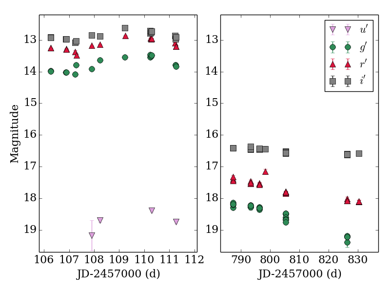
Figure 3: LCOGT lightcurve in $u^{\prime}$, $g^{\prime}$, $r^{\prime}$, and ${}^{\prime}i$ filters. Given the long time span between the two datasets, the outburst and post-outburst phases have been separated. The magnitudes are calibrated using SDSS data. We highlight the change in color of the object in the post-outburst phase.

The object was also tracked at the Beacon Observatory, associated with the University of Kent. The observatory is equipped with a 17” Astrograph and 4kx4k CCD with 0.956 arcsec/pixel. The filters are standard Johnson V, R_c, and I_c. The observations were taken on a fair-weather basis between November 2016 and January 2017. Exposure times range from 2 to 48 minutes, depending on the brightness of the star and the weather conditions. The data were corrected for bias and flat fielding, and an astrometric solution was obtained. Aperture photometry was calibrated relative to the data from JD=2457717.59 (estimated to be the best night in terms of weather and seeing), following an iterative procedure (Sicilia-Aguilar et al., 2008). Each filter was calibrated independently, and the final errors include photometry and relative calibration errors. The relative calibrations are found to be very stable and do not show any strong magnitude- or color dependency. No absolute calibration was possible in this case due to the lack of reference data.

Further data were provided by amateur astronomers R. Pickard and G. Piehler from the citizen science project HOYS-CAPS at the University of Kent. These data come from various sources, including their own telescopes and further LCOGT data. The data from Pickard were taken with the LCOGT 0.4, 1.0, and 2.0m telescopes. Thus, although most of the data were obtained for the VR_cI_c and VRI Bessell filters, there are some $r^{\prime}$ and $i^{\prime}$ data that are comparable to the rest of our LCOGT data, and thus calibrated in the same way. The data from Piehler were taken with a 510/2030mm Newtonic telescope with coma-corrector and a STL 11000M CCD camera. Data reduction was done with MAXIM DL 6.06. The filters used were a green TG filter and a clear filter CV. Although they are not identical to the Johnsons V filter, they are similar enough and can be used to display the overall evolution of the object during its return to quiescence. All the amateur data were calibrated against the best night observations from Beacon Observatory (or against LCOGT data, for the $r^{\prime}$ and $i^{\prime}$ observations from Pickard), and the results are fully consistent with them. Table 3 provides the results, which are displayed in Figure 4.

Table 3: Final calibrated photometry from the Beacon Observatory.

JDave	V	R	I
	(mag)	(mag)	(mag)
2457693.042a	13.97$\pm$0.03	13.58$\pm$0.05f	14.24$\pm$0.05f
2457702.610	13.57$\pm$0.21b	12.95$\pm$0.23b	13.93$\pm$0.18b
2457702.548a	13.70$\pm$0.03	—	—
2457703.506	13.64$\pm$0.03	13.31$\pm$0.03	14.03$\pm$0.11
2457707.143	—	—	15.04$\pm$0.06
2457717.594∗	14.14$\pm$0.01	13.84$\pm$0.01	14.51$\pm$0.01
2457722.452	14.04$\pm$0.05b	13.71$\pm$0.05b	14.41$\pm$0.05b
2457726.564	13.80$\pm$0.02	13.35$\pm$0.06	14.06$\pm$0.02
2457727.543	13.71$\pm$0.04	13.29$\pm$0.05	14.00$\pm$0.06
2457743.436a	14.50$\pm$0.06f	—	—
2457743.461a	14.38$\pm$0.06f	—	—
2457763.448	14.50$\pm$0.08	14.12$\pm$0.09	14.82$\pm$0.07
2457767.441	15.05$\pm$0.05	14.85$\pm$0.06	15.35$\pm$0.05
2457768.367	15.30$\pm$0.09	14.88$\pm$0.11	15.39$\pm$0.08
2457771.329	15.45$\pm$0.13	14.85$\pm$0.17	15.66$\pm$0.12
2457772.393	15.77$\pm$0.07	15.48$\pm$0.07	15.96$\pm$0.07
2457773.375	15.90$\pm$0.06	15.65$\pm$0.06	16.01$\pm$0.07
2457774.329	16.15$\pm$0.07	15.86$\pm$0.07	16.15$\pm$0.07
2457775.330	16.39$\pm$0.13	15.93$\pm$0.18b	16.22$\pm$0.10
2457780.296	—	16.39$\pm$0.19b	16.60$\pm$0.12
2457778.833a	16.15$\pm$0.10f	—	—
2457788.294a	17.78$\pm$0.13f	—	—
2457798.325a	17.50$\pm$0.17	—	—
2457800.275a	17.49$\pm$0.10f	—	—

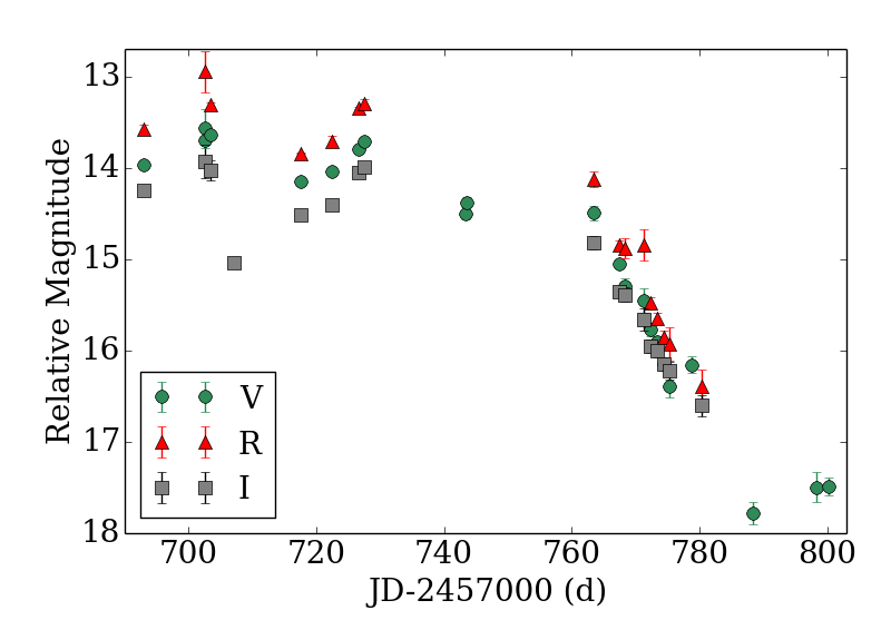
Figure 4: Light curve from the Beacon Observatory. The magnitudes are relative to the data from JD=2457717.594. The data show the rapid decrease of the source flux during January and February 2017 and stabilization from February to March 2017.

2.2 Spectroscopy

Table 4: Summary of spectroscopy observations.

JD	Date	Instrument	V	Phase
			(mag)
2456976.798	2014-11-15	CHIRON	13.7	0.168
2456978.808	2014-11-17	CHIRON	14.0	0.653
2456991.737	2014-11-30	CHIRON	14.0	0.771
2456991.753	2014-11-30	CHIRON	14.0	0.775
2456992.606	2014-12-01	CHIRON	13.5	0.981
2456992.797	2014-12-01	CHIRON	13.5	0.027
2456978.794	2014-11-17	FEROS	14.0	0.649
2456990.665w	2014-11-29	FEROS	13.7	0.513
2456995.700w	2014-12-04	FEROS	13.8	0.727
2457779.662	2017-01-26	OSMOS	16.5	0.816

A total of nine spectra were taken during the outburst. Six of them were taken with CHIRON (Tokovinin et al., 2013), a highly stable cross-dispersed echelle spectroscope deployed at the SMARTS 1.5m telescope. The remaining three were taken using the Fiber-fed Extended-Range Optical Spectrograph (FEROS; Kaufer et al., 1999), located at the European Southern Observatory/Max-Planck Gesellschaft (ESO/MPG) telescope in La Silla, Chile. Our CHIRON data have a resolution of R = 25,000 and a wavelength coverage from 4200 to 8800 Å. FEROS has a resolution of R = 48,000 and wavelength coverage $\sim$3700-9215 Å (Kaufer et al., 2000). The coverage is not continuous, with FEROS having a gap at 8860-8880 Å, while the CHIRON data is distributed over 61 orders with gaps between most of them. The observations were performed during November-December 2014 (see Table 4).

The reduction of the 1800 s-exposure FEROS spectra was performed using the FEROS pipeline, which involves de-biasing, flat fielding, extraction, and wavelength calibration. The CHIRON data were obtained in fiber mode and reduced with the CHIRON pipeline (e.g., Buysschaert et al., 2017). Due to the source being relatively faint for a 1.5m telescope, the CHIRON data are noisier than the FEROS spectra. The emission lines observed in the high-resolution data, identified using both CHIRON and FEROS datasets, are given in Section 4.

The lines were classified using line lists observed in other young stars (Sicilia-Aguilar et al., 2012; Appenzeller et al., 1986; Hamann & Persson, 1992) and the National Insitute of Standards and Technology (NIST) database for atomic spectra (Ralchenko et al., 2010). We excluded the parts of the spectrum affected by strong telluric emission and absorption features (Curcio et al., 1964), which affects about 60 lines. A total of 31 lines were not found within the NIST database, and thus appear as ‘INDEF’. Among these, 5 have also been observed in EX Lupi and likely correspond to strong transitions whose species have not yet been identified. The atomic constants of the lines (lower energy level E_i, upper energy level E_k and transition probability A_ki) were extracted from the NIST database. The complete line list is shown in Table LABEL:alllines-table. In total, we identify over 200 lines, about half of which are classified as ”strong”. Although this number is lower than the number of lines cited by Holoien et al. (2014), this is due to the worse S/N of the high-resolution spectra. We estimate that a further $\sim$200 lines are present but hard to identify due to blends, S/N, and/or atmospheric contamination.

Towards the end of the outburst ( January 26, 2017), when the object had an approximate magnitude of V=16.5 mag, a 3$\times$600s further spectrum was obtained with the 2.4m Hiltner Telescope and the low-resolution spectrograph Ohio State Multi-Object Spectrograph (OSMOS; R$\sim$1600; Martini et al., 2011), covering an approximate wavelength range between 3900 and 6800 Å. The wavelength solution has shifts up to $\sim$2.7 Å  which results in some uncertainties in the line identification. Although the object had nearly the same V magnitude as at the end of the 2013 outburst, the Hiltner spectrum is still dominated by continuum and narrow emission lines, similar to the spectrum obtained during the 2013 outburst (Holoien et al., 2014) or during the small outbursts of EX Lupi (Herbig et al., 2001; Sicilia-Aguilar et al., 2015). The results from the low-resolution spectroscopy are discussed in Section 3.5.

3 Basic properties during outburst and quiescence

3.1 Basic properties of ASASSN-13db

The basic properties of ASASSN-13db were revealed by Holoien et al. (2014), using photometry and spectra taken during the quiescence phase after the 2013 outburst. The star has a spectral type M5, which for its age and luminosity corresponds to a mass $\sim$0.15 M_⊙ and a radius $\sim$1.1 R_⊙. We adopt these values throughout the paper, although our data suggest a slightly lower radius (or luminosity) after the 2014-17 outburst (see Section 3.3).

The distance to ASASSN-13db is likely similar to the distance to the Orion complex, usually estimated to be 400-450 pc (Jeffries, 2007; Reid et al., 2009), but more recently suggested to be $\sim$390 pc (Kounkel et al., 2017). The distance of ASASSN-13db can be refined based on two arguments. First, the young star RX J0510.3-0330, at $\sim$2^′ from ASASSN-13db, has a distance of 370$\pm$34 pc estimated from GAIA (Gaia Collaboration et al., 2016, 2016). Second, the dark cloud Lynds 1616 is located near ASASSN-13db. We estimate the distance of Lynds 1616 using the 3D extinction map from Green et al. (2015). With 5-band $grizy$ Pan-STARRS 1 (Chambers et al., 2016; Flewelling et al., 2016) photometry and 3-band 2MASS $JHK_{\rm s}$ photometry (Cutri et al., 2003) of stars embedded in the dust, Green et al. (2015) trace the extinction on $7^{\prime}$ scales out to a distance of several kpc, by simutaneously inferring stellar distance, stellar type, and the reddening along the line of sight. Figure 5 shows the median cumulative reddening in each distance modulus (DM) bin within 0.1^∘ of the densest region of Lynds 1616. There is a rapid increase in the extinction at DM$\sim$7.5-8, suggesting a distance of 360$\pm$40 pc. Assuming that both RX J0510.3-0330 and Lynds 1616 belong to the same molecular cloud complex as ASASSN-13db, the distance of ASASSN-13db is likely $\sim$380 pc.

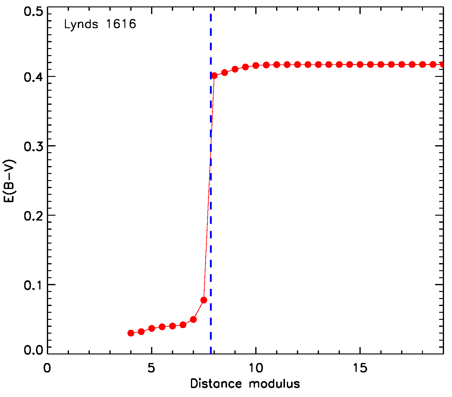
Figure 5: The median cumulative reddening in each distance modulus bin within 0.15^∘ of the densest region in Lynds 1616, using the data from Green et al. (2015). The dashed line marks the most likely distance for Lynds 1616.

3.2 Characteristics of the outburst spectrum

The spectra of classical T Tauri stars (CTTS) are characterized by numerous emission lines (Appenzeller et al., 1986; Hamann & Persson, 1992), with EXor variables being especially line-rich (Herbig et al., 2001). The high number of metallic lines observed during the ASASSN-13db outbursts is remarkable and uncommon for CTTS, but similar to what has been observed in EX Lupi (Kóspál et al., 2008; Sicilia-Aguilar et al., 2012; Holoien et al., 2014). The strongest line is H$\alpha$, with wings extending to $\pm$300 km/s, followed by other lines typical of accretion processes such as the Ca II IR triplet. Neutral and ionized Fe lines make up most of the emission spectrum. Most of the lines have low excitation potentials and correspond to features usually observed in absorption in the photospheres of late-type stars. Their upper level energies, E_k, are in the range 2.4-6.7 eV, as observed in EX Lupi (Sicilia-Aguilar et al., 2012) and V1118 Ori (Giannini et al., 2017) during outburst. Other neutral and ionized lines observed include Mg I/II, Ca I, Cr I, Co I, Ni I, Si II, V I, and Ti I/II.

Many lines have a strong, redshifted, absorption component with a width $\sim$100-200 km/s, together with a blue-shifted emission component $\sim$50-150 km/s in width. Such profiles are classified as inverse P-Cygni or YY Ori-type profiles and are typical of systems viewed at high inclination angles (near edge-on), where the temperature in the accretion flow decreases at larger distances from the star, and infalling matter is seen along the line-of-sight, leading to higher-velocity material and potential obscurations of the star by the disk and the magnetosphere. The disk does not necessarily need to be edge-on with respect to the disk unless the accretion columns are polar, which may not be the case. For instance, in EX Lupi, the accretion spots in quiescence appear to hit the star at $\sim$50 degrees latitude (Sicilia-Aguilar et al., 2015), so for ASASSN-13db the angle may be high, but the line-of-sight does not necessarily have to go through the disk or disk edge.

Table 5: Emission lines observed during the outburst. The lines are classified as “strong” (S) or “weak” (W). The “References” indicate whether the line has been observed in the 2013 outburst (H14; Holoien et al., 2014), or in EX Lupi, either in outburst (SA12; Sicilia-Aguilar et al., 2012) or quiescence (SA15; Sicilia-Aguilar et al., 2015). Uncertain classifications (due to several lines being consistent with the same wavelength, or to mismatches between observed and potential laboratory wavelengths) are marked with ‘Unc.’. For some of these lines, a second possible species may be responsible: these are given in the ‘Comments’ column. Lines that appear blended with others are labeled as ‘Ble.’. Lines that could not be associated with any known transition are listed as ‘INDEF’. Lines affected by atmospheric contamination are marked with ‘Atm.’, and INDEF lines observed in EX Lupi are also labeled. Finally, lines for which the strong, wind-related blue-shifted absorption is seen are marked with ‘BA’.

Species	Wavelength (Å)	Strength	References	Comments
H I	4861.28	S	SA12,H14,SA15	H$\beta$ absorption
H I	6562.57	S	SA12,H14,SA15	BA
H I	8413.32	W	SA12
H I	8437.95	W	SA12
H I	8467.26	S	SA12	Ble.
H I	8750.46	W	SA12
H I	9014.91	S	SA12	Unc. Atm.
Ca I	5041.62	S
Ca I	6450.86	W		Unc.
Ca II	8248.80	W	SA15
Ca II	8498.02	S	SA12,H14,SA15
Ca II	8542.09	S	SA12,H14,SA15
Ca II	8662.14	S	SA12,H14,SA15
Na I	5889.95	W	SA12,H14,SA15
Na I	5895.63	W	SA12,H14,SA15
C I	9088.57	S	SA12	Ble. Atm.
O I	8446.25	W	SA12,SA15	Unc.
Mg I	5167.32	S	SA15	BA
Mg I	5172.68	S	SA15
Mg I	5183.6	S	SA15
Mg I	5711.09	W
Mg I	8806.76	S		Ble.
Mg II	4390.59	W
K I	7664.90	W		Atm.
S II	6312.42	W		Ble.
Si II	5957.56	S	SA12
Si II	6347.10	S	SA12,SA15
Si II	6371.36	W	SA12,SA15
Ti I	6312.03	S
Ti I	7069.07	S		Unc.
Ti I	8623.43	S		Atm.
Ti II	4417.72	W	SA12,SA15	Unc.
Ti II	4468.50	W	SA12,SA15	Unc. Ble.
Ti II	4529.47	S	SA12
Ti II	4571.98	S	SA12,SA15
Ti II	5129.15	S	SA12
Ti II	5226.56	S	SA12
V I	5727.78	W		Unc.
V I	6324.66	S	SA12
V I	8203.07	S		Atm. Ble.
Co I	7016.62	S	SA12	Unc.
Co I	7085.10	S		Ble.
Cr I	4077.09/.68	W	SA12	Unc.
Cr I	5204.52	S	SA12
Cr I	5208.44	W	SA12
Cr I	5298.27	S	SA12
Cr I	6138.24	S
Ni I	5753.69	S
Fe I	4045.82	W	SA12,SA15	Unc., BA
Fe I	4063.55	W	SA12,SA15	Unc., BA
Fe I	4071.74	W	SA12,SA15	Unc.
Fe I	4132.06	W	SA12,SA15
Fe I	4191.43	W	SA12,SA15
Fe I	4207.13	W	SA12	Ble.
Fe I	4208.60	W	SA12	Ble.
Fe I	4215.42	W	SA12
Fe I	4226.34	W	SA12	Unc., BA
Fe I	4258.61	W	SA12	Unc.
Fe I	4293.80	S	SA12	Ble.
Fe I	4324.95	W	SA12,SA15
Fe I	4325.74/.76	W	SA12,SA15
Fe I	4375.93/.99	S	SA12,SA15
Fe I	4383.55	S	SA12,SA15	BA
Fe I	4389.24	W
Fe I	4408.41	W	SA12
Fe I	4415.12	W	SA12,SA15
Fe I	4461.65	S	SA12,SA15
Fe I	4482.17	S	SA12,H14
Fe I	4494.46	W	SA12,H14,SA15
Fe I	4602.94	S	SA12
Fe I	4772.80	S	SA12	Unc.
Fe I	4939.24/.69	S	SA12
Fe I	4994.13	S	SA12	Fe II 4993.36?
Fe I	5012.07	S	SA12
Fe I	5041.07/.76	S	SA12	Ca I 5041.62?
Fe I	5051.63	S	SA12
Fe I	5060.03	S	SA12
Fe I	5083.34	S	SA12
Fe I	5110.36	S	SA12
Fe I	5123.72	S	SA12
Fe I	5151.90	S	SA12
Fe I	5227.15/.19	S	SA12
Fe I	5247.05	S	SA12
Fe I	5250.65	S	SA12
Fe I	5254.95	S	SA12
Fe I	5263.31	S	SA12
Fe I	5267.20	W		Ble.
Fe I	5269.50/70.36	S	SA12,SA15
Fe I	5328.04/.53	S	SA12,SA15
Fe I	5332.90	S	SA12
Fe I	5341.02	S	SA12
Fe I	5371.49	W	SA12,SA15
Fe I	5397.13	S	SA12, SA15
Fe I	5455.61	S	SA12,SA15
Fe I	5497.52	S	SA12
Fe I	5501.47	S	SA12
Fe I	5508.41	S	SA12
Fe I	5709.38	W	SA12	Ble.
Fe I	5732.30	W	SA12	Ble.
Fe I	5753.12/.69/5.35	S	SA12	Ble.
Fe I	5816.06/.37	S	SA12	Ble.
Fe I	5835.50/.57	W	SA12	Ble.
Fe I	5853.68	W	SA12
Fe I	5859.61	W
Fe I	5862.36	W	SA12
Fe I	5916.25	S	SA12	Ble.
Fe I	5958.33	S	SA12
Fe I	5976.78	W	SA12	Ble.
Fe I	5984.81	W	SA12	Ble.
Fe I	6008.56	W	SA12
Fe I	6065.48	S	SA12	Ble.
Fe I	6116.04	W
Fe I	6127.91	S	SA12	Ble.
Fe I	6173.34	W	SA12
Fe I	6191.56	S	SA12	Ble.
Fe I	6200.31	S	SA12
Fe I	6230.72	W	SA12
Fe I	6232.64	W	SA12	Ble.
Fe I	6254.26/6.13	S	SA12	Blend
Fe I	6297.79	S	SA12	Unc. Atm.
Fe I	6318.02	S	SA12	Ble.
Fe I	6336.82	S	SA12
Fe I	6393.60	S	SA12	Unc.
Fe I	6400.00	S	SA12	Unc.
Fe I	6408.02	S	SA12
Fe I	6411.65	S	SA12
Fe I	6421.35	S	SA12	Ble.
Fe I	6498.94	S	SA12
Fe I	6546.24	S	SA12,H14	Unc.
Fe I	6574.10	S	H14	Ble.
Fe I	6609.11	S	SA12,H14
Fe I	6705.12	W		Ble.
Fe I	6750.15	W	SA12	Unc.
Fe I	6769.66	S		Ble.
Fe I	6841.34	S	SA12	Ble.
Fe I	6945.20	S	SA12	Atm.
Fe I	6978.85	S	SA12	Ble.
Fe I	7024.06	S	SA12
Fe I	7223.66	S	SA12	Ble. Atm. Unc.
Fe I	7914.712	S		Atm.
Fe I	7937.14	W	SA12	Unc.
Fe I	8027.94	W	SA12	Atm.
Fe I	8048.99	S
Fe I	8075.56	S
Fe I	8220.38	W	SA12	Ble., Atm.
Fe I	8327.06	S	SA12	Atm., Unc.
Fe I	8514.07	S		Unc.
Fe I	8582.26	W	SA12
Fe I	8824.22	S	SA12
Fe I	9147.71/.96	S
Fe II	4233.17	S	SA12,SA15	Unc.
Fe II	4273.33	W	SA12,SA15	BA
Fe II	4351.77	W	SA12,SA15	Unc.
Fe II	4489.18	S	SA12,SA15
Fe II	4549.47	S	SA12,SA15
Fe II	4629.34	S	SA12,SA15	Ti II 4629.47?
Fe II	4666.76	W	SA12,SA15
Fe II	4731.45	W	SA12,SA15	Var.
Fe II	4923.92	S	SA12,SA15	BA
Fe II	5018.43	S	SA12,SA15	BA
Fe II	5080.31	S		Fe I 5080.35?
Fe II	5316.61	S	SA12,SA15
Fe II	5534.85	W	SA12,SA15
Fe II	6113.32	W	SA12
Fe II	6247.56	W	SA12,SA15
Fe II	6432.68	S	SA12
Fe II	6456.38	W	SA12,SA15
Fe II	6516.05	S	SA12,H14,SA15
Fe II	6678.88	S
Fe II	7111.71	W		Unc.
Fe II	7462.38	S	SA12
Fe II	7711.26/.71	S	SA12	Ble.
Fe II	8839.06	W		Unc.
INDEF	4428	S
INDEF	5430	S
INDEF	5498	S
INDEF	5743	W
INDEF	5911	S		FeI 5914?
INDEF	5992	S	SA12
INDEF	6331	W		FeI 6335?
INDEF	6534	W
INDEF	6266	S	SA12
INDEF	6772	S
INDEF	6786	W		Ble.
INDEF	6808	W
INDEF	6816	W
INDEF	6989/90	S
INDEF	7001	S
INDEF	7039	S
INDEF	7054	W		Atm.
INDEF	7197	S		Atm.
INDEF	5395	S		Ble., Fe I 5393?
INDEF	5793	W	SA12
INDEF	7724	W
INDEF	7749	S	SA12	Ble.
INDEF	7790	S
INDEF	8366	S
INDEF	8389	S	SA12	Fe I 8387.71?
INDEF	8403	W
INDEF	8676	S
INDEF	8758	S		Atm.
INDEF	8945	S		Ble.
INDEF	8977	W		Atm.
INDEF	9103	W		Atm.
INDEF	9211	S		He I?

Ionized (Fe II, Ti II) lines correspond to relatively hot gas and are common in accreting, low-mass stars (e.g., Hamann & Persson, 1992). Comparing to EX Lupi and other higher-mass EXors and accreting TTS, the most surprising characteristic of ASASSN-13db is the lack of strong He I lines, which are usually among the strongest emission lines observed in CTTS (Hamann & Persson, 1992). Like EX Lupi (Sicilia-Aguilar et al., 2012), ASASSN-13db shows no evidence for the forbidden lines common in CTTS (Hamann, 1994), which could indicate that there is no shock or that the density of the surrounding material is high ($>$10⁵ cm^-3) so that the shock is quenched (Nisini et al., 2005). Examples of the typical velocity profiles are shown in Figure 6, and Table 6 lists the strongest lines observed. Another interesting feature of ASASSN-13db is the absence of H$\beta$ emission. Although the H$\alpha$ line shows prominent emission and a mild redshifted absorption asymmetry, H$\beta$ appears as a mildly redshifted absorption feature (see Figure 7). The lack of He I and H$\beta$ emission could be a consequence of the high inclination (thus resulting in occultation of the hottest parts of the accretion shock, as observed in EX Lupi in outburst for high-energy lines; Sicilia-Aguilar et al., 2015) or to low temperatures in the accretion structures associated with ASASSN-13db, in contrast with solar-mass stars, as has also been suggested for brown dwarfs (Scholz et al., 2009; Bozhinova et al., 2016). These possibilities are discussed in Section 4.3.

Table 6: Strong lines used to derive the accretion properties.

Species	$\lambda$	Ei	Ek	Aki	Notes
	(Å)	(eV)	(eV)	(s-1)
Fe I	4375.930	0	2.83	2.95E+04	F
Fe I	4461.652	0.08	2.87	2.95E+04	F
Fe I	4482.169	0.11	2.88	2.09E+04
Ti II	4571.980	1.57	4.28	1.92E+07	F
Fe I	4602.941	1.48	4.18	1.72E+05	F
Fe II	4923.921	2.89	5.41	4.28E+06	F, BA
Fe II	5018.434	2.89	5.36	2.00E+06	F, BA
Fe I	5060.034	4.3	6.75	—
Fe I	5083.338	0.95	3.4	4.06E+04
Fe I	5110.358	3.57	6.0	9.99E+05
Ti II	5129.150	1.89	4.31	1.46E+06	F
Mg I	5167.32	1.48	3.88	2.72E+06	F, BA
Mg I	5172.684	2.71	5.11	3.37E+07	F
Fe I	5332.899	1.55	3.88	4.36E+04
Fe I	5341.024	1.6	3.93	5.21E+05
Fe I	5397.127	0.91	3.21	2.58E+04
Fe I	5455.609	1.01	3.28	6.05E+05
Fe I	5506.779	0.99	3.24	5.01E+04	F
Fe I	5916.247	2.45	4.55	2.15E+04
Si II	5957.560	10.06	12.15	5.60E+07
Fe I	5958.333	2.17	4.26	—
Fe II	5991.376	3.15	5.22	4.20E+03	F
Fe I	6191.558	2.43	4.43	7.41E+05	F
Fe I	6200.312	2.61	4.61	9.06E+04	F
Fe I	6336.824	3.87	5.64	7.71E+06
Si II	6347.100	8.12	10.07	5.84E+07
Fe I	6393.601	2.43	4.37	4.81E+05
Fe I	6400.001	3.6	5.54	9.27E+06	F
Fe I	6421.351	2.28	4.21	3.04E+05
Fe I	6498.939	0.96	2.87	4.64E+02
H$\alpha$	6562.57	10.2	12.09	5.39E+07	BA
Fe II	6678.883	10.93	12.79	2.40E+07	F
Fe I	6750.152	2.42	4.26	1.17E+05
Fe I	6978.851	2.48	4.26	1.44E+05
Fe I	8048.990	4.14	5.68	—
H I	8467.26	12.1	13.55	3.44E+03
Ca II	8498.020	1.69	3.15	1.11E+06	F
Fe I	8514.07	2.19	3.65	1.09E+05
Ca II	8542.09	1.69	3.15	9.90E+06
Ca II	8662.140	1.69	3.12	1.06E+07
Mg I	8806.756	4.36	5.75	1.27E+07
Fe I	8824.221	2.19	3.6	3.53E+05	F

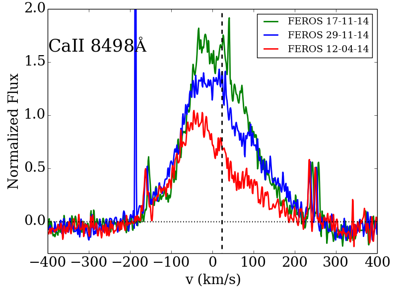
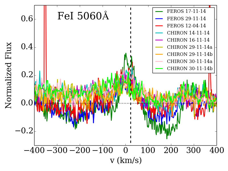
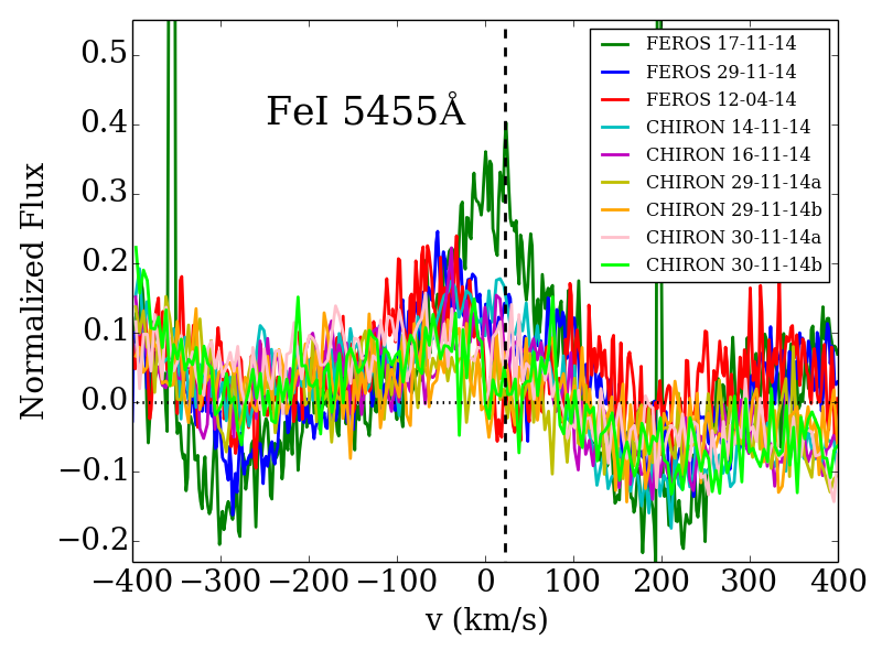
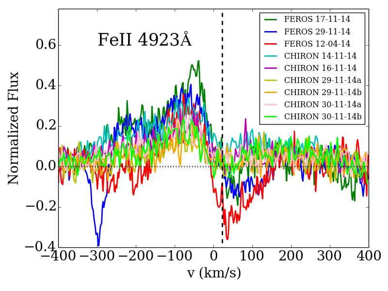
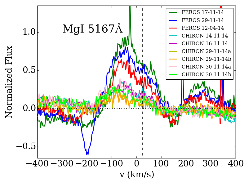
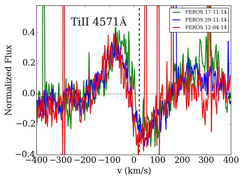
Figure 6: Structure of several metallic neutral and ionized lines in the FEROS and CHIRON spectra during outburst. The dashed line marks the radial velocity of ASASSN-13db.

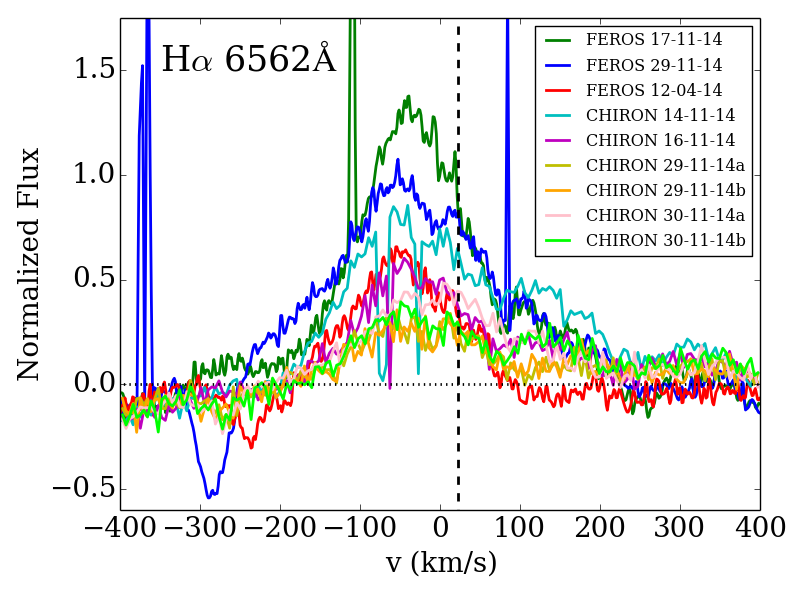
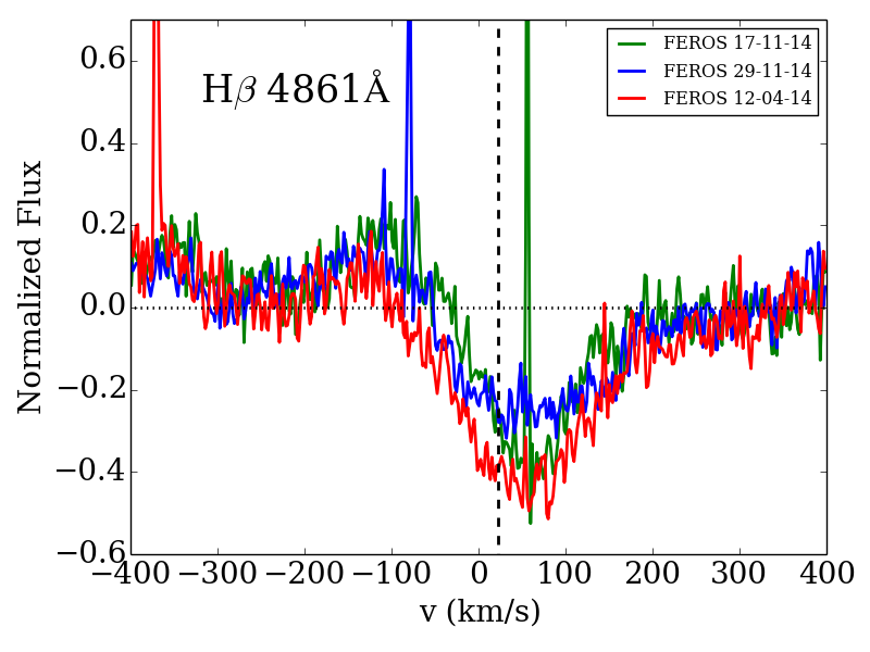
Figure 7: Normalized and continuum-subtracted H$\alpha$ (top) and H$\beta$ (bottom) lines as observed with FEROS and CHIRON (we note that H$\beta$ is only covered by FEROS). While the H$\alpha$ line has a strong, asymmetric, emission component, H$\beta$ appears only in absorption. The dashed line marks the radial velocity of ASASSN-13db.

3.3 Accretion rate estimates

The best way to measure the accretion rate during outburst is via the accretion luminosity. To estimate the total luminosity, we assume that the bulk emission resembles that of a star with an earlier spectral type. This is usually the case for FUor objects (Hartmann & Kenyon, 1996), and it was observed for ASASSN-13db during the 2013 outburst (Holoien et al., 2014), for EX Lupi (Juhász et al., 2012), and many other EXors (Lorenzetti et al., 2012). We then integrate the outburst spectral energy distribution (SED) observed by the LCOGT. Given that the 2014-2017 outburst is stronger than the 2013 one, we take the 2013 outburst temperature (4800K; Holoien et al., 2014) as a lower limit. Temperatures below $\sim$4800 K would result in either very unrealistic luminosities or extremely large radii. Similarly, temperatures in excess of $\sim$7000 K result in effective radii that are too small, which gives us our upper limit. As seen in Figure 8, temperatures around 4800-5800 K produce the best fits. Since we assume that extinction is negligible (in agreement with Holoien et al., 2014) and a black-body SED, the luminosities may be underestimated. Line emission may also affect the observed magnitudes (Juhász et al., 2012). The luminosities derived are around 0.5-0.6 L_⊙, with the best fit being 0.6 L_⊙. After the 2017 outburst, the estimated luminosity drops to 0.03 L_⊙, which is lower than the 0.06 L_⊙ measured by Holoien et al. (2014). In general, the luminosity appears lower than the average for a M5 star (Fang et al., 2017), which may indicate a slightly later spectral type or variable extinction not accounted for at this stage since the difference is minimal compared to the outburst luminosity. The luminosity obtained is very similar to the result derived from the ASAS-SN mean outburst magnitude (13.71$\pm$0.40 mag), assuming a distance of 380 pc and using the bolometric corrections for young stars from Kenyon & Hartmann (1995).

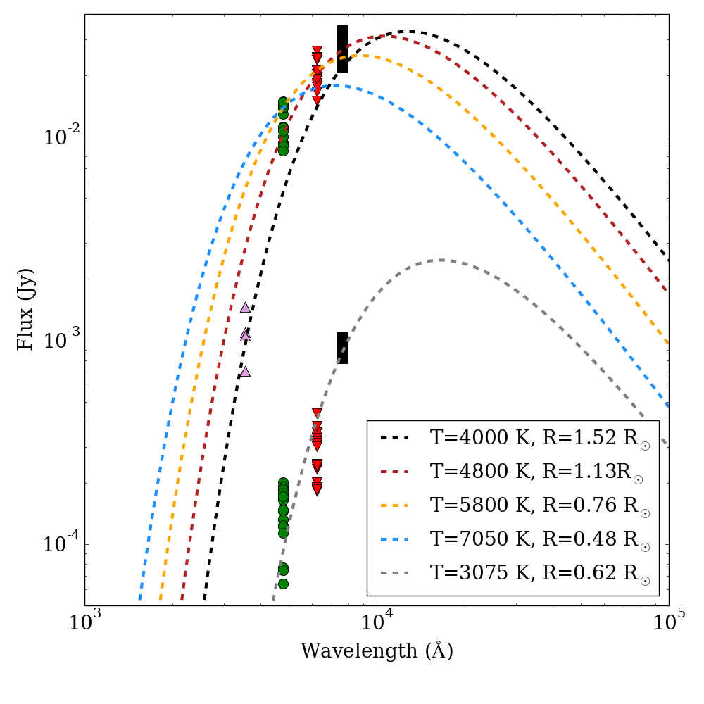
Figure 8: SED fits to the LCOGT data in outburst and quiescence. Black bodies with different temperatures and effective radii are displayed for comparison.

The accretion luminosity can be translated into an accretion rate following Gullbring et al. (1998),

$$L_{acc}=\frac{GM_{star}\dot{M}}{R_{star}}\left(1-\frac{R_{star}}{R_{infall}}\right),$$ (1)

where G is the gravitational constant, Ṁ is the accretion rate, and R_infall is the typical infall radius (taken to be 5 R_star by Gullbring et al., 1998). From this, we can estimate an accretion rate in the range Ṁ=0.9-1.5 $\times$ 10^-7 M_⊙/yr, or about Ṁ=0.7-3.3 $\times$ 10^-7 M_⊙/yr if we account for the observed span in magnitudes (Figure 8) and the uncertainty in the stellar mass and radius. The same reasoning using the peak magnitude during the 2013 outburst ($\sim$0.5 mag fainter) and an effective temperature of 4800 K suggests that the accretion rate in 2013 was about half of the value observed in the 2014-2017 outburst.

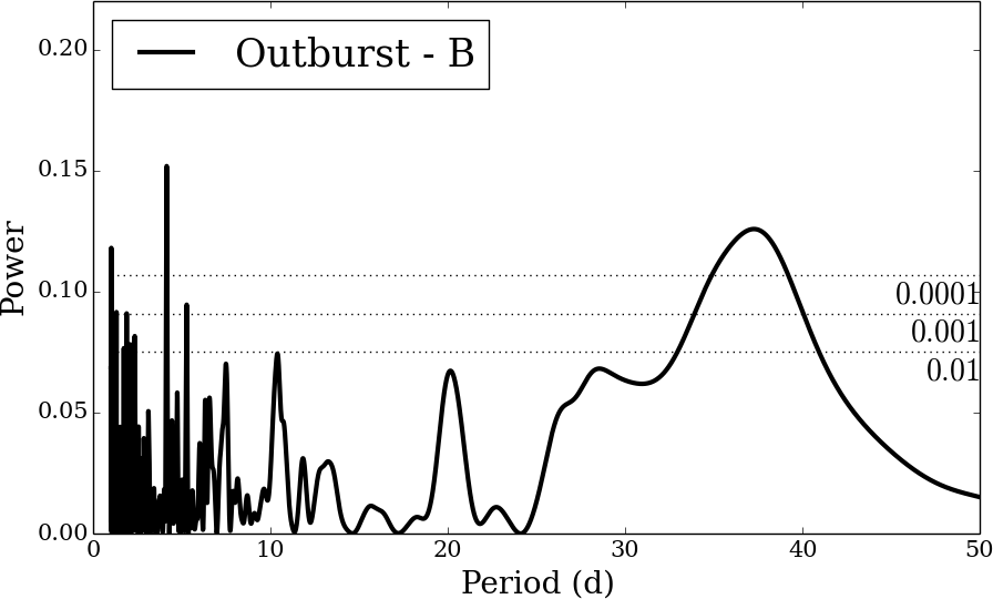
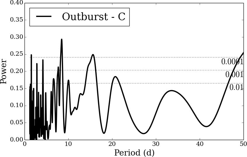
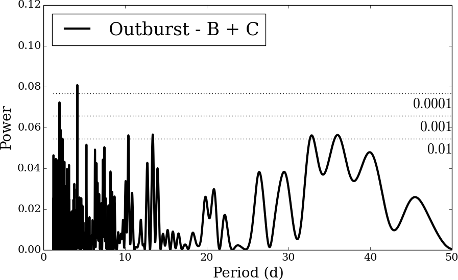
Figure 9: GLSP periodograms for the 2014-2017 outburst during different epochs within the outburst phase.

During the post-outburst phase, we use the integrated line fluxes to derive the accretion rate from the flux-calibrated OSMOS spectrum. Following the transformations between line luminosity and accretion luminosity from Fang et al. (2009), we use the H$\alpha$, H$\beta$, and the He I 5875Å line fluxes to derive the accretion luminosity, and then Equation 1 to derive the accretion rate. The results are mutually consistent (Table 7), with an average of Ṁ_{post-outburst}=(1.2$\pm$0.2)$\times$10^-9 M_⊙/yr. The uncertainty in this value could be of a factor of few, taking into account the assumptions for the infall radius and the spread in the accretion rate versus line flux relations (Fang et al., 2009). This accretion rate is on the high end for stars with similar stellar masses (Fang et al., 2009; Manara et al., 2017), but it may be enhanced with respect to the true quiescence value since the underlying stellar spectrum is still heavily veiled. In summary, ASASSN-13dbs experienced an increase in the accretion rate of over two orders of magnitude between quiescence and outburst, which is similar to or higher than the increase in accretion observed for EX Lupi in its 2008 outburst (Sicilia-Aguilar et al., 2012; Juhász et al., 2012).

Table 7: Post-outburst line luminosities and accretion rates.

Line	Lline	Lacc	Ṁ
	(L⊙)	(L⊙)	(M⊙/yr)
H$\alpha$	2.0e-4	4.5e-3	1.4$\times$10-9
H$\beta$	5.3e-5	3.4e-3	1.0$\times$10-9
He I 5875Å	4.7e-6	4.3e-3	1.3$\times$10-9

3.4 Periodicities during the outburst phase

The temporal coverage of the ASAS-SN data allows us to search for periodicity in the light curve. For this, we run a generalized Lomb-Scargle periodogram (GLSP; Scargle, 1982; Horne & Baliunas, 1986; Zechmeister & Kuerster, 2009). Since the light curve is substantially different during the 2013 outburst, we restricted our study to the 2014-2017 data. We then explored the GLSP for the three parts of the outburst separated by observability gaps using the Python lomb_scargle routine. Figure 9 shows the periodograms taken during epochs B and C, when significant periodic signatures are detected. The first dataset (A) shows a quasi-periodic signal of about 12.6$\pm$0.6 d, with several other peaks. Dataset B reveals a strong periodic signal (false-alarm probability, FAP$<$10^-7) at 4.15$\pm$0.05 d, which also appears as a clear modulation in the phase-folded magnitude (see Figure 10), with an amplitude of about 0.5 magnitudes and a large scatter. The same period, within errors, is also recovered in dataset C (4.20$\pm$0.09 d) and from the combination of datasets B and C (4.15$\pm$0.03 d). Although the main peaks of the power spectrum in dataset A, A+B, or in the whole data are different, they all have peaks around 4.1-4.2 d. The combination of all epochs has a potential periodic signal of 10.39$\pm$0.07 d. Both the 12.6 and the 10.4 d could be resonances or aliases of the 4.15 d signature (3:1,5:2). A similar phenomenon has been observed by Mortier & Collier Cameron (2017): signals at resonant periods tend to appear when the number of stellar spots (which would correspond to accretion columns in our case) varies or when they are evolving. It could be thus interpreted as changes in the accretion structures during the beginning of the outburst, in epoch A, followed by a more stable accretion phase until the end of the outburst. Folding the data by the longer periods does not lead to any conclusive results or shows quasi-periodic modulations only in a small subset of data, and some FAP may be underestimated due to red noise. Table 8 summarizes the results.

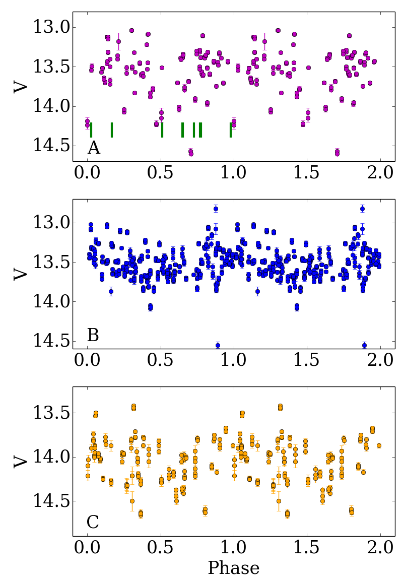
Figure 10: Phase-folded ligth curve for the A, B, and C periods of ASAS-SN observations (see text) assuming a 4.15$\pm$0.05 d period. The data are repeated to display two phases. The phases at which the FEROS and CHIRON spectra were obtained are marked as vertical green lines.

The 4.15 d period and the observed modulation are similar to those expected from rotational modulation of a star with an asymmetric and slowly variable distribution of spots. Considering a M5 spectral type and 1-2 Myr age, we can expect a mass of approximately 0.15$\pm$0.05 M_⊙ according to Siess et al. (2000). In this mass and age range, 4.15 d is within typical rotation rates (Herbst et al., 2002; Lamm et al., 2005; Littlefair et al., 2010; Scholz, 2013; Bouvier et al., 2014). The modulations observed in the LCOGT and Kent data during outburst are also consistent with the 4.15d period (see Figure 11), although none of the datasets contain enough points to allow for an independent estimate of the period. The fact that the shape and phase of the curve seems to change slightly with epoch may be due to slow changes in the spot distribution (possibly related to evolution of the accretion columns) throughout the outburst, although the uncertainties in the period over long time spans may also contribute.

Table 8: Observed periods during the 2014-2017 outburst and their false-alarm probabilities (FAP).

Epochs	Period	FAP	Comments
	(d)
A	1.531$\pm$0.007	$<$5e-5	Alias?
”	12.66$\pm$0.61	$<$1e-4	3:1 Resonance?
”	2.856$\pm$0.029	$<$1e-4	2:3 Resonance?
B	4.146$\pm$0.045	$<$1e-7	Strong
C	8.42$\pm$0.43	$<$1e-4	2:1 Resonance?
”	4.200$\pm$0.095	$<$2e-3
A + B	4.141$\pm$0.015	$<$1e-6
”	10.376$\pm$0.084	$<$1e-6	5:2 Resonance?
B + C	4.147$\pm$0.028	$<$1e-4
All	12.63$\pm$0.10	$<$1e-6	3:1 Resonance?
”	10.386$\pm$0.066	$<$1e-6	5:2 Quasi-periodic
”	4.144$\pm$0.012	$<$5e-6
”	6.321$\pm$0.024	$<$5e-6	3:2 Resonance?

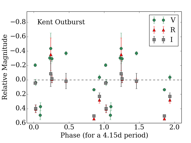
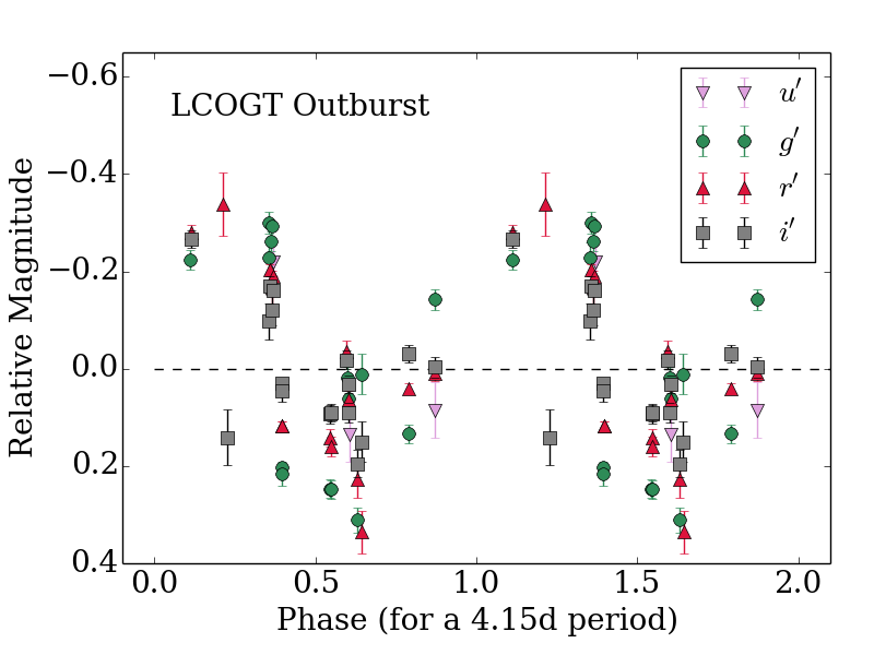
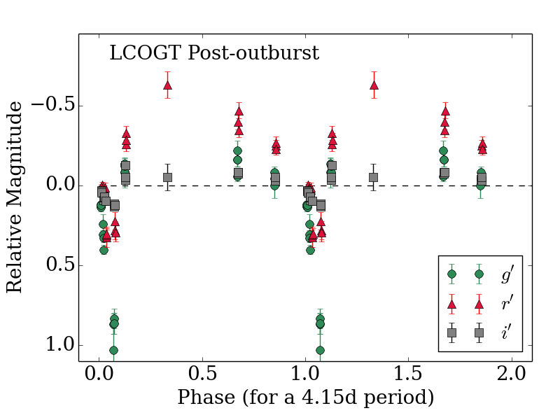
Figure 11: Top: Phase-folded light curve for the data from the Beacon Observatory, using the 4.15d period. Middle: Phase-folded light curve for the LCOGT data during outburst. Bottom: Phase-folded light curve for the LCOGT data during the post-outburst. All datasets are repeated to show two complete phases, and scaled to the average magnitudes. We note the phase shift between the datasets, which could be due to evolution of the spots. The color change in the post-outburst phase may show a brief occultation event in the $g^{\prime}$ band.

3.5 The end of the outburst

When the object became observable in September 2016, it had decreased in brightness by about 0.5 mag, compared to epoch B of the outburst, and was slowly declining. In December 2016, ASAS-SN and Beacon Observatory data showed that the magnitude was rapidly decreasing. By February 2017 the object had reached the previous quiescence levels, terminating the outburst after nearly 800 days. The last results from the LCOGT (March 2017) indicate that the object is still experiencing a very slow magnitude decrease and changes in color (see Figure 3), meaning that the steady state may not have been reached yet.

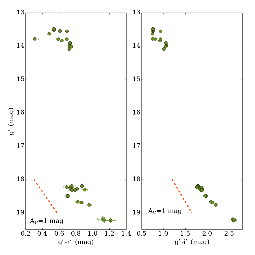
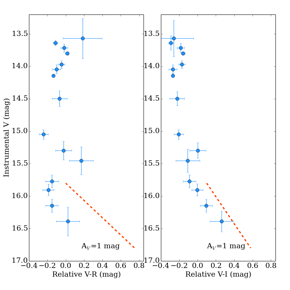
Figure 12: Color-magnitude diagrams showing the color evolution as observed by the LCOGT (left) and the Beacon Observatory (right). For the Kent data, since the different filters are not cross-calibrated, the colors are shifted around the median value and only the relative color variation is relevant. A reddening vector (Cardelli et al., 1989; Stoughton et al., 2002) is shown for comparison.

The color evolution of ASASSN-13db can be studied with the LCOGT and Kent data (see Figure 12). The LCOGT data covers part of the high and low states in all $g^{\prime},r^{\prime},i^{\prime}$ bands, while the Kent data sample most of the dimming with data taken between November 2016 and February 2017; in the last part of the outburst, however, we could only obtain V data (thus no colors are available) at Kent. Although the Kent filters are not cross-calibrated, the data provides valuable information about the dimming process and the relative color evolution. The colors reveal that a luminosity change by approximately four magnitudes occurs at nearly constant color, and thus cannot be attributed to extinction. The colorless magnitude change could be caused by an extended hot-spot region shrinking as the accretion rate decreases, followed by cooling down towards the M5 spectrum. Similar color changes, including a substantial colorless magnitude decrease, have been observed in other outbursting stars such as V1118 Ori (Audard et al., 2010). At the last stage of the outburst, the object experiences a rapid color change, becoming redder faster than expected from extinction alone. If the outburst phase is dominated by hot continuum ($>$4800 K) and the quiescence state is dominated by the emission of a M5 star (T_eff=3075 K), the source should become significantly redder even in the absence of extinction, with a color change of about 1 mag in V-R_c and about 2.5 mag in V-I_c (using the colors for young Taurus stars from Kenyon & Hartmann, 1995), which are larger than observed. The typical Sloan colors for M5 stars also suggest that the object will likely evolve to redder magnitudes ($g^{\prime}-r^{\prime}$=1.43 mag, $g^{\prime}-i^{\prime}$=3.21 mag for a M5 star according to Fang et al., 2017). As of March 2017, it appears that the star is still dimming and evolving in color, and we predict that it will likely be redder in quiescence.

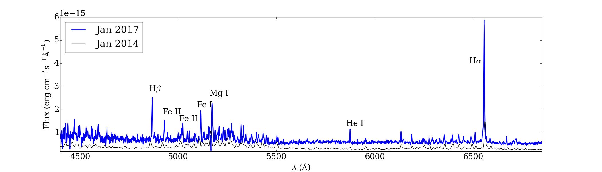
Figure 13: The post-outburst low-resolution OSMOS spectrum (blue), compared to the 2013 post-outburst data (black). Some of the strongest lines are labeled. We note that the stellar photospheric features were not visible as of January 2017.

The OSMOS spectrum taken near the end of the outburst (Figure 13) shows no evidence of self-absorption or complex line structure except in the H$\alpha$ line. Despite the low resolution ($\sim$50 kms^-1/pix), the deep and broad absorption features observed in outburst would be still visible if they were present. Identification of weak or blended lines is highly uncertain due to the low resolution, so we list only the strongest lines (see Table 9). H$\alpha$ is the only line that appears asymmetric, with a redshifted absorption that does not go below the continuum level. H$\beta$ and He I 5875Å are now detected in emission, suggesting that higher temperature regions become visible as the accretion column becomes less optically thick. This was also observed in EX Lupi, where the higher-energy lines become visible during quiescence (Sicilia-Aguilar et al., 2015). Although the object had faded back to V$\sim$16.6 mag when the spectrum was taken, the photosphere of the M5 star was not visible yet, and the spectrum still resembled those from the 2013 outburst with strong, relatively narrow, emission lines.

Table 9: Strong lines observed in the post-outburst phase.

Species	$\lambda$	References
	(Å)
CrI:	4078	SA15
FeII	4351	SA15
H$\beta$	4861	SA12/SA15
FeI/FeII	4939/4924	SA12/SA15
FeII	5018	SA12/SA15
FeI	5027	SA12
FeI	5050	SA12
FeI	5056	SA12
FeI:	5110	SA12
MgI	5173	SA15/SA12
HeI	5876	SA15/SA12
FeI/CrI	6137/6138	—
FeI:	6180	SA12
FeI	6355	SA12/H14
FeI	6394	SA12/H14
FeI	6426	SA12/H14
CaI/FeII	6451/6456	H14/SA12
CaI	6494	H14/SA12
FeII	6516	H14/SA12
H$\alpha$	6563	SA12/SA15
NiI/[NII]/CI	6586/6583/6588	SA12/H14/SA15
FeII/HeI	6679/6678	H14/SA12/SA15

4 Accretion structure from spectroscopy

4.1 Line velocity auto- and cross-correlations

The complexity of the emission lines requires a pixel-by-pixel analysis of the line structure, which can be done by exploring the velocity-space via auto- and cross-correlations (Alencar et al., 2001; Sicilia-Aguilar et al., 2015). The emitted flux at each velocity is cross-correlated with the flux at any other velocity, for either the same line (auto-correlation), or for another line (cross-correlation). This requires having numerous spectra with high S/N, which reduces our sample to the very bright lines that are well-detected by both FEROS and CHIRON and that are not blended with other lines within $\pm$300 km/s. By assigning each velocity bin to a gas parcel moving at a given rate, the connection between parts of the system is revealed by the auto- (and cross-) correlation matrix. This approach allows us to explore the lines in a non-parametric way, which is particularly useful for very complex lines such as H$\alpha$. The main limitation is that there can be several independent gas parcels moving at the same velocity with respect to our line of sight (e.g., due to projection, or due to the presence of more than one accretion column).

We focused on H$\alpha$ and Fe II 4923 Å as representative examples of the emission-only and strong inverse P-Cygni profiles. Lines from the same multiplet (e.g., Fe II 4923Å and 5018 Å) have nearly identical profiles and velocity structure (as observed in EX Lupi Sicilia-Aguilar et al., 2012). To construct the correlation matrices, the FEROS spectra were first resampled to the CHIRON resolution. For each line, a local normalization was performed, measuring the continuum on both sides of the line in regions not affected by other features. We then obtained the auto-(cross-)correlation matrix by correlating each line pixel-by-pixel with itself (a different line). We used customized Python routines based on the Spearman rank correlation to derive a correlation coefficient, r, and the false-alarm probability, p.

Figure 14 shows the results of the correlations. The auto-correlation for the H$\alpha$ line reveals a complex asymmetry with a strong correlation between the blue- and red-shifted sides. The correlation coefficient between the line wings and the center of the line decreases rapidly, suggesting that the zero-velocity gas components come from different or very extended locations. The cross-correlation matrix for H$\alpha$ and Fe II 4923Å shows a correlation between the central and blue-shifted part of the line. There are no evident correlations for line velocities between 0 and100 km/s, but the red-shifted side of H$\alpha$ is correlated with the blue-shifted side of Fe II 4923Å. A mild anticorrelation between the red-shifted wings in H$\alpha$ and the red-shifted Fe II absorption suggests that the absorption becomes deeper when the H$\alpha$ line wings are stronger. This is in agreement with an increase of the material along the line-of-sight, supporting the classification as a nearly edge-on YY Ori system. Being more extended and associated with lower temperatures, H$\alpha$ would increase at the same time as the self-absorption in the Fe II lines increases. There is no further evidence of relative correlations between the lines nor between the absorption and wind components other than the general correlation that all lines tend to get stronger (or weaker) in parallel.

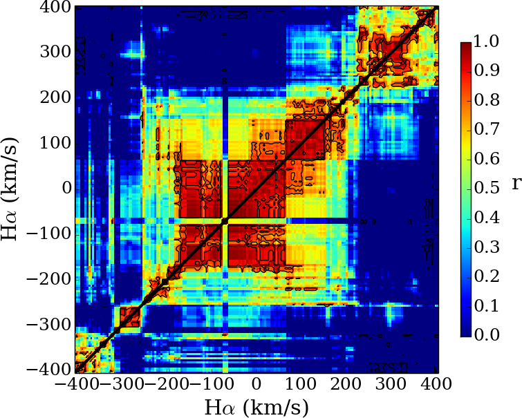
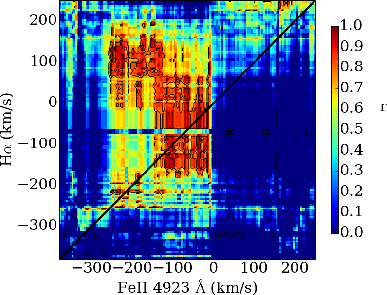
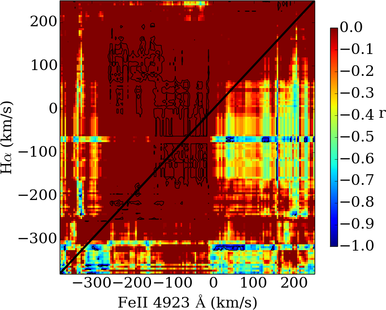
Figure 14: Auto-correlation (left) and cross-correlation of H$\alpha$ with the Fe II 4923Å line; including positive (middle) and negative (right) correlations. The color scheme shows the value of the Spearman rank correlation parameter r, and the black contours mark the high-significance areas with false-alarm probability 1e-3 and 1e-4, respectively.

4.2 Line velocity structure

To study the line structure, we need to estimate the radial velocity of ASASSN-13db. The complexity of the emission line profiles and the lack of any reliable photospheric absorption line in the high-resolution spectra do not allow for a direct determination, so we adopt as a reference the velocities of the L1615 and L1616 clouds in Orion (22.3$\pm$4.6 km/s; Gandolfi et al., 2008), which are roughly similar to the average radial velocities in the ONC ($\sim$25-30 km/s; Sicilia-Aguilar et al., 2005). The lines show strong day-to-day variability in both intensity and structure.

Besides the inverse P-Cygni profile, the FEROS data from November 29, 2014 and December 4, 2014 reveal deep, blueshifted absorption features in several of the lines, including the H$\alpha$, Fe I, and Fe II lines (see Figures 7 and 6 and Table LABEL:alllines-table). The velocity of the blueshifted absorption changes by about $\geq$50 km/s between the two dates, being about $\sim-$300 km/s on November 29, 2014 and between $\sim-$250/$-$200 km/s on December 4, 2014. Although there are small differences in the velocity from line to line, the general behavior is consistent. Blueshifted absorption lines are usually ascribed to winds. In this case, the rapid velocity change of the line at roughly fixed strength is suggestive of rotational modulation in a non-axisymmetric wind. The FEROS spectrum from November 17, 2014 does not have blueshifted absorption features below the continuum, although it has a clear absorption feature that dominates the blue wing of the line (see Figure 7). The CHIRON spectra taken on November 30, 2014 (between the two FEROS spectra) have a marginal wind absorption feature, but it is hard to establish because of the low S/N. There is no apparent correlation between the wind and the rotation phase, with the wind being observed at phase 0.51 and 0.73, but not at 0.65. This suggests a strong, variable wind in addition to the effects of rotation and geometry. More data would have been desirable to confirm the wind geometry.

We restrict the velocity and structure analysis to lines that are strong and unblended over at least a $\pm$200 km/s region around the line, and that are well-identified (i.e., we cannot reasonably attribute the same line to more than one species). We also restrict our analysis to the metallic lines, excluding H$\alpha$, which has a very complex profile. We concentrate on the high S/N FEROS data.

To perform a quantitative analysis of the line profile, we first fit the emission with a multi-Gaussian profile (as had been done for EX Lupi; Sicilia-Aguilar et al., 2012, 2015, see also Appendix A). The emission lines of ASASSN-13db are more complex than those of EX Lupi (which consist of well-defined broad and narrow components), so the fits are used to quantify the line in terms of the intensities and velocities of the emission and absorption components, and the emission line width (see Figure 15). Although the three-Gaussian components are highly degenerate, the general line parameters derived are very robust, and we do not observe any differences (within their errors) when derived from different three-Gaussian fits. They include the normalized flux peak (F_max) and its velocity (V_max), the velocity (V_min) and depth (F_min) of the redshifted absorption, the maximum velocity of the absorption feature (V_redsh; calculated as the maximum redshifted velocity at which the absorption correspond to 10% of the maximum absorption), and the width at 10% of the peak in the emission component (W_10%). Some lines are well-fitted with only two Gaussians. For the lines where the absorption component is not present, the line parameters related to absorption are not computed. The errors in the derived quantities depend on the S/N of the spectrum and the line width. Errors in the maximum and minimum flux are estimated based on the average S/N within the emission or absorption feature. Errors in the velocities are derived accordingly from the Gaussian fit, taking into account the peak and minimum flux errors. The uncertainties in W_10% and V_redsh are derived considering the errors in the peak and minimum flux with respect to which they are measured.

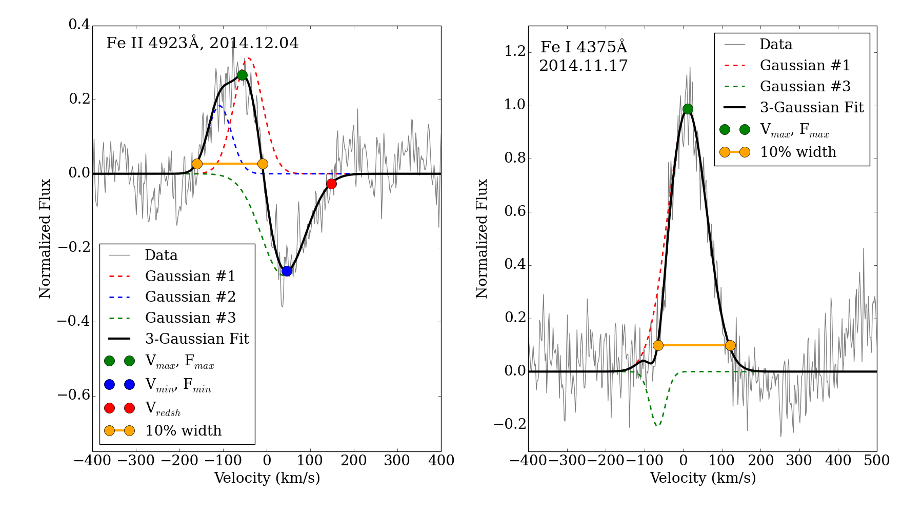
Figure 15: Some examples of the three-Gaussian fits and the quantities derived from them. We note that the Fe I 4375Å line can be fitted with only two Gaussians, and does not include absorption component parameters.

We used these quantifiers of the line shapes to explore potential correlations between the atomic parameters (including the energies of the upper and lower levels, the transition probability, and the sum of the ionization and excitation potentials; Bertout et al., 1982) and the line emission and absorption properties. The strength of the correlation was determined using the Spearman rank test, which produces a correlation coefficient (r) and a false-alarm probability (p) for each pair of variables. Negative correlation coefficients mean that the quantities are anticorrelated. Among all non-trivial possibilities, five strong correlations (p$\leq$0.005; see Figure 16) and six marginal correlations (p$\sim$0.006-0.06) arise, listed in Table 10. Considering the line parameters themselves, we find five further correlations. Three of them are trivial (e.g., all the velocities are correlated, indicating that lines tend to globally shift in velocity), while two marginal correlations suggest that stronger lines tend to be more redshifted, and that shallower absorption features tend to appear at larger redshifted velocities (see Appendix B).

Table 10: Correlations and marginal correlations found between the line properties and atomic parameters.

Correlated quantities	r	p	Comments
Vmax vs Ek	$-$0.36	0.02	marginal
Vmax vs Aki	$-$0.63	5e$-$6
Vmax vs Total Exc.	$-$0.61	7e$-$6
Fmax vs Ei	$-$0.31	0.04	marginal
Fmax vs Ek	$-$0.39	0.01	marginal
Fmax vs Total Exc.	$-$0.39	0.009	marginal
Vmin vs Ek	$-$0.34	0.06	marginal
Vmin vs Aki	$-$0.47	0.005
Vmin vs Total Exc.	$-$0.66	3e$-$5
Vredsh vs Aki	$-$0.47	0.009	marginal
Vredsh vs Total Exc.	$-$0.51	0.004
Vmin vs Vmax	0.77	1e$-$7
Vmax vs Vredsh	0.68	3e$-$5
Vmax vs Fmax	0.35	0.02	marginal
Vmin vs Vredsh	0.70	1e$-$5
Vmin vs Fmin	0.31	0.08	marginal

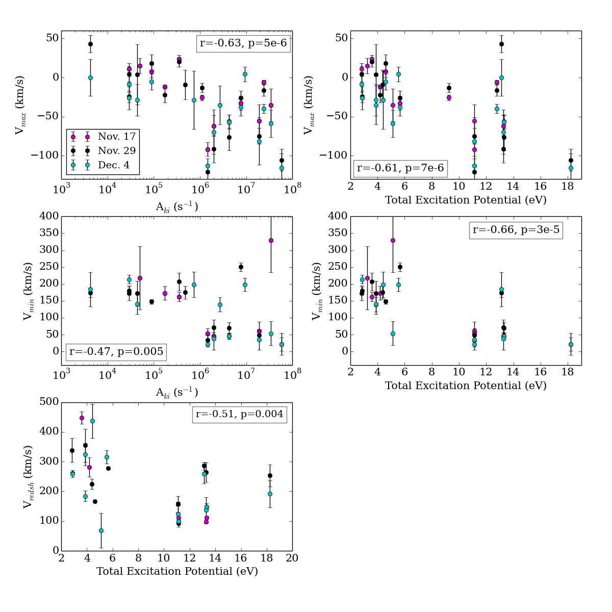
Figure 16: Strong correlations between the line profiles and different atomic parameters. The correlation coefficient (r) and the false-alarm probabilities (p) for the Spearman rank correlation are given in the plots. See text for details.

We find anticorrelations between the transition probability (A_ki) and the line velocities (for the peak velocity, V_max, the velocity at maximum absorption, V_min, and the zero redshifted velocity, V_redsh). The lines with higher transition probabilities appear more blue-shifted. Similar anticorrelations arise between the total excitation potential (the sum of the ionization potential, which is zero for neutral lines, and the energy of the upper level) and the line velocities (V_max, V_min, V_redsh). The lines with lower excitation potentials are more strongly redshifted. Surprisingly, this is opposite to the behavior found for other systems with YY-Ori-type line profiles, such as SCrA and CoD-35^o10525, for which Bertout et al. (1982) and Petrov et al. (2014) found that lines formed at low temperatures are strongest at low infall velocity. In our case, the anticorrelation between the total excitation potential and the velocity of maximum absorption rather indicates that the highest infall velocities are reached for the lines formed at lower temperatures. Optical depth and geometrical considerations (such as more absorbing material in the more distant locations, which also would display lower infall velocities, or occultation of the hottest and densest parts of the flow due to the inclination) could play a role here. One solution to produce a density inversion would be to accumulate material away from the star (for instance, at the edge of the magnetosphere). Hot spots associated with magnetic reconnection, which have been suggested to explain high-energy variability in eruptive stars (Hamaguchi et al., 2012), could also produce high density, high temperature, low velocity structures. In any case, more observations (including high-energy data, magnetic mapping, and high-resolution, high S/N spectroscopy) would be required to explore this possibility.

Table 11: Line velocity structure and atomic parameters (from NIST) for the high S/N lines. Line absorption parameters are fit only when the line has a redshifted absorption.

Species	Ei	Ek	Eion	Aki	Vmax	Fmax	Vmin	Fmin	W10%	Vredsh
	(eV)	(eV)	(eV)	(s-1	(km/s)		(km/s)		(km/s)	(km/s)
2014.11.17
FeI 4375.93	0.00	2.83	0.00	2.95E+04	11$\pm$8	0.989$\pm$0.011	—	—	186$\pm$4	—
TiII 4571.98	1.57	4.28	6.83	1.92E+07	$-$56$\pm$21	0.339$\pm$0.062	61$\pm$27	$-$0.259$\pm$0.056	128$\pm$23	157$\pm$26
TiII 5129.15	1.89	4.31	6.83	1.46E+06	$-$92$\pm$9	0.468$\pm$0.016	53$\pm$16	$-$0.106$\pm$0.017	140$\pm$8	111$\pm$12
FeI 4602.94	1.48	4.18	0.00	1.72E+05	$-$12$\pm$3	0.514$\pm$0.006	173$\pm$21	$-$0.034$\pm$0.007	228$\pm$4	282$\pm$33
FeII 4923.92	2.89	5.41	7.90	4.28E+06	$-$56$\pm$8	0.336$\pm$0.006	46$\pm$9	$-$0.155$\pm$0.009	283$\pm$6	112$\pm$5
FeII 5018.43	2.89	5.36	7.90	2.00E+06	$-$62$\pm$13	0.348$\pm$0.012	45$\pm$11	$-$0.222$\pm$0.018	222$\pm$15	98$\pm$3
MgI 5172.68	2.71	5.11	0.00	3.37E+07	$-$35$\pm$21	0.375$\pm$0.032	329$\pm$96	$-$0.110$\pm$0.018	204$\pm$28	669$\pm$129
FeI 5506.78	0.99	3.24	0.00	5.01E+04	15$\pm$10	0.440$\pm$0.018	217$\pm$94	$-$0.038$\pm$0.010	138$\pm$9	538$\pm$154
FeI 6200.31	2.61	4.61	0.00	9.06E+04	8$\pm$8	0.522$\pm$0.008	—	—	201$\pm$7	—
FeI 6336.82	3.87	5.64	0.00	7.71E+06	$-$33$\pm$9	0.512$\pm$0.012	—	—	179$\pm$9	—
FeI 6678.88	10.93	12.79	0.00	2.40E+07	$-$6$\pm$3	0.680$\pm$0.003	—	—	221$\pm$2	—
CaII 8498.02	1.69	3.15	6.11	1.11E+06	$-$26$\pm$3	1.642$\pm$0.007	—	—	297$\pm$5	—
FeI 8824.22	2.19	3.60	0.00	3.53E+05	24$\pm$5	0.733$\pm$0.007	162$\pm$14	$-$0.233$\pm$0.004	135$\pm$2	448$\pm$21
2014.11.29
FeI 4375.93	0.00	2.83	0.00	2.95E+04	5$\pm$10	0.431$\pm$0.006	173$\pm$21	$-$0.068$\pm$0.008	338$\pm$11	339$\pm$40
FeI 4461.65	0.08	2.87	0.00	2.95E+04	$-$24$\pm$8	0.387$\pm$0.005	180$\pm$12	$-$0.167$\pm$0.007	321$\pm$19	261$\pm$4
TiII 4571.98	1.57	4.28	6.83	1.92E+07	$-$75$\pm$10	0.276$\pm$0.010	48$\pm$12	$-$0.283$\pm$0.009	144$\pm$7	158$\pm$7
TiII 5129.15	1.89	4.31	6.83	1.46E+06	$-$121$\pm$10	0.275$\pm$0.010	34$\pm$15	$-$0.080$\pm$0.012	155$\pm$6	92$\pm$11
FeI 4602.94	1.48	4.18	0.00	1.72E+05	$-$22$\pm$10	0.313$\pm$0.006	900$\pm$42	$-$0.047$\pm$0.001	235$\pm$6	—
FeII 4923.92	2.89	5.41	7.90	4.28E+06	$-$76$\pm$17	0.336$\pm$0.011	70$\pm$17	$-$0.130$\pm$0.015	277$\pm$18	148$\pm$11
FeII 5018.43	2.89	5.36	7.90	2.00E+06	$-$91$\pm$18	0.265$\pm$0.016	72$\pm$23	$-$0.186$\pm$0.013	189$\pm$15	264$\pm$32
FeI 5332.90	1.55	3.88	0.00	4.36E+04	4$\pm$38	0.098$\pm$0.032	172$\pm$37	$-$0.165$\pm$0.026	184$\pm$63	355$\pm$56
FeII 5991.38	3.15	5.22	7.90	4.20E+03	43$\pm$11	0.172$\pm$0.005	174$\pm$13	$-$0.093$\pm$0.005	174$\pm$7	286$\pm$13
FeI 6200.31	2.61	4.61	0.00	9.06E+04	18$\pm$11	0.267$\pm$0.006	148$\pm$7	$-$0.049$\pm$0.013	212$\pm$9	167$\pm$4
FeI 6336.82	3.87	5.64	0.00	7.71E+06	$-$26$\pm$9	0.426$\pm$0.004	251$\pm$13	$-$0.031$\pm$0.005	795$\pm$20	279$\pm$5
SiII 6347.10	8.12	10.07	8.15	5.84E+07	$-$105$\pm$14	0.178$\pm$0.015	22$\pm$20	$-$0.165$\pm$0.009	110$\pm$7	253$\pm$37
FeI 6393.60	2.43	4.37	0.00	4.81E+05	$-$9$\pm$19	0.337$\pm$0.029	175$\pm$19	$-$0.122$\pm$0.035	182$\pm$21	224$\pm$17
FeI 6678.88	10.93	12.79	0.00	2.40E+07	$-$16$\pm$8	0.369$\pm$0.001	—	—	294$\pm$4	—
CaII 8498.02	1.69	3.15	6.11	1.11E+06	$-$13$\pm$6	1.335$\pm$0.006	—	—	353$\pm$5	—
FeI 8824.22	2.19	3.60	0.00	3.53E+05	20$\pm$6	0.533$\pm$0.007	207$\pm$27	$-$0.185$\pm$0.004	144$\pm$3	525$\pm$28
2014.12.04
FeI 4461.65	0.08	2.87	0.00	2.95E+04	$-$26$\pm$15	0.402$\pm$0.037	214$\pm$13	$-$0.180$\pm$0.033	176$\pm$20	258$\pm$12
FeI 4375.93	0.00	2.83	0.00	2.95E+04	$-$8$\pm$10	0.401$\pm$0.014	—	—	384$\pm$24	—
TiII 4571.98	1.57	4.28	6.83	1.92E+07	$-$81$\pm$30	0.282$\pm$0.096	35$\pm$30	$-$0.314$\pm$0.091	135$\pm$40	123$\pm$29
FeII 4923.92	2.89	5.41	7.90	4.28E+06	$-$57$\pm$9	0.266$\pm$0.007	45$\pm$9	$-$0.262$\pm$0.007	151$\pm$4	148$\pm$5
FeII 5018.43	2.89	5.36	7.90	2.00E+06	$-$70$\pm$28	0.285$\pm$0.088	38$\pm$33	$-$0.229$\pm$0.091	164$\pm$30	137$\pm$44
TiII 5129.15	1.89	4.31	6.83	1.46E+06	$-$113$\pm$9	0.251$\pm$0.014	22$\pm$8	$-$0.117$\pm$0.012	115$\pm$10	99$\pm$6
MgI 5167.32	1.48	3.88	0.00	2.72E+06	$-$35$\pm$25	0.584$\pm$0.043	139$\pm$21	$-$0.155$\pm$0.073	264$\pm$34	184$\pm$18
MgI 5172.68	2.71	5.11	0.00	3.37E+07	$-$59$\pm$17	0.201$\pm$0.018	54$\pm$35	$-$0.005$\pm$0.036	173$\pm$25	69$\pm$58
FeI 5332.90	1.55	3.88	0.00	4.36E+04	$-$29$\pm$20	0.128$\pm$0.011	141$\pm$31	$-$0.104$\pm$0.011	226$\pm$67	325$\pm$37
FeII 5991.38	3.15	5.22	7.90	4.20E+03	0$\pm$23	0.079$\pm$0.023	184$\pm$50	$-$0.078$\pm$0.037	564$\pm$513	259$\pm$33
FeI 6191.56	2.43	4.43	0.00	7.41E+05	$-$29$\pm$37	0.102$\pm$0.017	198$\pm$38	$-$0.139$\pm$0.013	219$\pm$38	437$\pm$58
FeI 6200.31	2.61	4.61	0.00	9.06E+04	$-$6$\pm$10	0.183$\pm$0.004	—	—	205$\pm$7	—
FeI 6336.82	3.87	5.64	0.00	7.71E+06	$-$38$\pm$11	0.263$\pm$0.004	—	—	382$\pm$17	—
SiII 6347.10	8.12	10.07	8.15	5.84E+07	$-$116$\pm$19	0.124$\pm$0.016	22$\pm$32	$-$0.085$\pm$0.012	140$\pm$22	192$\pm$45
FeI 6400.00	3.60	5.54	0.00	9.27E+06	4$\pm$10	0.393$\pm$0.010	198$\pm$20	$-$0.102$\pm$0.009	171$\pm$8	316$\pm$22
FeI 6678.88	10.93	12.79	0.00	2.40E+07	$-$40$\pm$6	0.237$\pm$0.002	—	—	323$\pm$5	—

4.3 Accretion column properties derived from the emission lines

For stars with a large number of emission lines, it is possible to determine the physical conditions (temperature and density) in the accretion columns by using line ratios of neutral and ionized lines (Beristain et al., 1998; Sicilia-Aguilar et al., 2012, 2015). Although the S/N for most of the data is too low to perform a velocity-dependent analysis, the relative intensities can be explored for a number of lines. As with EX Lupi, we can constrain the approximate density in the accretion column based on the observed typical accretion rate Ṁ=2$\times$10^-7M_⊙/yr. This accretion rate would result from the mass within the volume of the accretion column multiplied by the approximate density. The volume that is accreted onto the star per second can be approximated by the typical velocity of the infalling material ($v\sim 40$ km/s) multiplied by the cross-section of the column(s). Therefore, the accretion rate can be written as

$$\dot{M}=\mu\,n\,v\,f4\pi R_{*}^{2},$$ (2)

where $n$ is the density, $\mu$ is the mean atomic weight, $f$ is the fraction of the stellar surface covered by spots (in general, a small part of the stellar surface, 1-20% Calvet & Gullbring, 1998; Lima et al., 2010), and R_∗ is the stellar radius (1.1$R_{\odot}$ as estimated by Holoien et al., 2014). These values imply a particle (mostly H) density in the range n$\sim$2$\times$10¹³-4$\times$10¹⁴ cm^-3. If we assume that, at the relevant temperatures in the accretion column, hydrogen and helium will be mostly neutral and all the metals will be singly ionized, then the electron density will be a factor of 1000 lower, n${}_{e}\sim$2$\times$10¹⁰ to 4$\times$10¹¹ cm^-3.

An independent constraint on the electron density can be obtained from the saturation of the Ca II IR triplet lines (Hamann & Persson, 1992). For the Ca II IR lines to have similar strength, collisional decay (given by C_ki) must dominate over the radiative transition rate (A_ki), which requires n_eC${}_{ki}\gg$A_ki/$\tau$. This imposes a relation between the opacity and the electron density of $\tau$ n${}_{e}\gtrsim$ 10¹³ cm^-3 for Ca II 8542/8662Å. Considering that usually $\tau>$1-10 (Grinin & Mitskevich, 1988; Shine & Linsky, 1974), we arrive to an approximate value for n${}_{e}\sim$ 10¹² cm^-3. These values are slightly higher than those derived from the accretion rate. In the case of EX Lupi, the mismatch between accretion-based estimates and the requirements for Ca II saturation was attributed to higher levels of ionization than expected due to UV radiation from the accretion shock. For ASASSN-13db, we expect less ionizing radiation due to the lower mass of the system, and both values agree within a factor of few. The accretion columns could also be significantly optically thicker for the case of a small object viewed nearly edge-on, so the differences are reasonable given the uncertainties.

Several lines can be used to constrain the temperature and density. If we assume local thermodynamical equilibrium, the relative populations of ions and neutrals is determined by the Saha equation (Saha, 1921; Mihalas, 1978)

$$\frac{N_{j+1}n_{e}}{N_{j}}=\left(\frac{2\pi mkT}{h^{2}}\right)^{3/2}\frac{2U_{j+1}(T)}{U_{j}(T)}e^{-\chi_{I}/kT}.$$ (3)

Here, N_j+1, N_j, and n_e represent the number of atoms in the j+1 and j ionization states and the electron number density, T is the temperature, m is the electron mass, $\chi_{I}$ is the ionization potential, and U_j+1 and U_j are the partition functions for the j+1 and j states. The level populations follow a Boltzmann distribution, and can be transformed into line intensity ratios to compare with the observed data. Using the density threshold imposed by the Ca II emission, we used the Saha equation (together with the data available from NIST; Ralchenko et al., 2010) for several line pairs to further constrain the temperature and density.

The lack of He I emission also constrains the temperatures within the accretion flow. The He I line at 5875Å is commonly observed in accreting, low-mass stars (Hamann & Persson, 1992; Sicilia-Aguilar et al., 2005). Temperatures around 20000 K are required to thermally excite the He I line, which suggests that the accretion shock/flow in ASASSN-13db is cooler than in solar-type objects.

Ti I/Ti II lines are another strong indicator of temperature. For a temperature of 6500 K, Ti I emission disappears unless the density is high (n${}_{e}\sim$ 1$\times$10¹⁴ cm^-3). A temperature of 5000 K would require a density of around n${}_{e}\sim$ 3$\times$10¹¹ cm^-3, while for 5800 K, the expected density for substantial Ti I emission would be n${}_{e}\sim$ 1$\times$10¹³ cm^-3. From the constraints derived from the accretion rate and the Ca II emission, we conclude that the temperature in the accretion structures is most likely below 6000 K.

The observed 1:2 Fe I 5269Å/Fe II 5169Å line ratio is also consistent with a temperature around 5800 K for a density in the range n${}_{e}\sim$5$\times$10¹¹-2$\times$10¹² cm^-3. These low temperatures in the accretion flow are consistent with the M5 spectral type of the object (Holoien et al., 2014), which for young stars lies close to the border between very-low-mass stars and brown dwarfs.

The lack of H$\beta$ emission is in agreement with this picture; according to the accretion flow models by Muzerolle et al. (2001), absorption in H$\beta$ appears at large inclinations ($\gtrsim$75 degrees) for a flow temperature of about 6000 K and an accretion rate around 10^-8M_⊙/yr (lower than we observe). Although the temperature is in agreement with our estimates, our accretion rate during the 2014-2017 outburst is substantially higher.

All these lines of evidence suggest that the dominant temperature in the flow is of the order of 5800-6000 K. Detailed line radiative transfer models, applied to this specific case of a very-low-mass object, should be explored in the future to address the line structure.

5 Discussion: the variable nature of ASASSN-13db

The 2013 and 2014-2017 outbursts of ASASSN-13db are significantly different. While the first outburst is in full agreement with typical EXor outbursts (e.g., Herbig et al., 2001), the second one is unusual in length and in magnitude. The length of the 2014-2017 outburst is shorter than typical FUors, although several FUor outbursts lasting only a few years have been observed (e.g., ZCMa, V1647 Ori, $[$CTF93$]$216-2; Fedele et al., 2007; Aspin, 2011; Caratti o Garatti et al., 2011; Audard et al., 2014; Bonnefoy et al., 2016). Objects with similar outburst lengths are often referred to as EXors, but this is typically accompanied by a question mark or considered as an intermediate case, especially if some FUor characteristics are present (e.g., Ábrahám et al., 2004; Fedele et al., 2007; Caratti o Garatti et al., 2011). Although ASASSN-13db experienced a slow decay after September 2016 (similar to the smooth, exponential-like decays observed in FUors; Hartmann & Kenyon, 1996), the final abrupt dimming and return to quiescence over $\sim$2 months is more typical of EXor behavior. The overall shape of the light curve (Figure 1) strongly resembles, in length, duration, and general shape (including the quick magnitude drop after a slow fading), that of the light curve of the FUor variable V1647 Ori (Fedele et al., 2007), the object that illuminated the McNeil nebula during its 2004 outburst (McNeil et al., 2004; Briceño et al., 2004). The 2010 outburst of the very-low-mass star [CTF93]216-2 (M_∗=0.25 M_⊙; Caratti o Garatti et al., 2011) also shares many characteristics with the ASASSN-13db 2014-17 outburst. An intermediate class, MNors, has been proposed for objects similar to the McNeil nebula (Contreras Peña et al., 2017), although for ASASSN-13db there is no evidence for a reflection nebula (see Figure 2), and the object appears less embedded than other MNors. The accretion rate observed in outburst ($\sim$2$\times$10^-7M_⊙/yr) and the increase of accretion between quiescence and outburst of at least two orders of magnitude are more in agreement with large EXor outbursts, such as the 2008 EX Lupi outburst (Sicilia-Aguilar et al., 2012; Juhász et al., 2012). If the second outburst corresponds to a FUor episode, it would be the first time that an object has been seen to undergo both types of behavior. ASASSN-13db would also be the lowest mass FUor object known to date, suggesting that accretion outbursts, like the rest of disk and accretion properties, occur in very-low-mass stars and perhaps substellar-mass objects.

Few-day periodic or quasi-periodic signatures, usually attributed to inner disk structures, are characteristic of FUor objects (e.g., Herbig et al., 2003; Siwak et al., 2013). For the periodic 4.15d signature to arise in the inner disk, we would need a disk structure located at about 0.09 au or about 20 R_⊙, assuming Keplerian rotation. Assuming T_eff=3075 K for a M5 star, with a radius of about 1.1 R_⊙ (Holoien et al., 2014), the temperature in this region would be of the order of $\sim$730 K (strongly dependent on dust properties and inner disk structure), which is fully compatible with the presence of silicate dust grains. However, if the typical temperature in outburst is higher ($>$4800 K), the disk temperature at 0.09 au would be at least 1100-1300 K, close to the silicate sublimation temperature of $\sim$1500 K. ASASSN-13db may be near edge-on or at a high angle, so extinction by accretion channels or extended accretion structures in the disk cannot be excluded. Nevertheless, the relatively smooth, colorless sinusoidal light curve is rather suggestive of modulations induced by accretion-related hot/cold spot(s), rather than periodic eclipses.

The detection of the 4.15 d period in data taken during a period of over 500 days (epochs B and C) suggests that the mechanism responsible for the variability is very stable, or has only experienced small variations during this time. A stable accretion structure has been observed in V1467 Ori (Hamaguchi et al., 2012) and EX Lupi (Sicilia-Aguilar et al., 2015). Very-low-mass objects are expected to have strong and mostly bipolar magnetic fields (Morin et al., 2010; Gregory et al., 2014), which could produce these structures. The modulation becomes undetectable in January 2017, once the light curve is dominated by a rapid decrease in magnitude, but appears to be again consistent with the small-scale variability observed in March 2017 (see Figure 11, bottom).

The variations in line depth and wind absorption suggest that both the accretion structures and the associated wind component are not uniformly distributed around the star. A non-axisymmetric location could explain the rapid, day-to-day variations in the velocity of the wind and redshifted absorption component due to rotation. Although rotational modulations induced by non-axisymmetric accretion columns are common (e.g., Costigan et al., 2012; Kurosawa & Romanova, 2013), wind modulations are rare. If associated with the accretion column, the observations of ASASSN-13db could be consistent with the X-wind scenario (Shu et al., 1994) or a jet originating at the magnetic reconnection point proposed to explain the high-energy variability of V1647 Ori (Hamaguchi et al., 2012). Further data is required to explore this possibility.

Despite the potentially high inclination of the disk (or, at least, a view of the accretion columns along the infall direction), several of the observations rule out the possibility that the observed behavior is caused by eclipses or occultations by disk material or UXor-type variability (e.g., Grinin et al., 1991; Natta et al., 1999). UXor variability can produce apparently ”high” states over long periods of time (Bouvier et al., 2013), but UXors present high extinction and trace a ”¿” shaped curve in the color-magnitude diagram, since the colors become bluer at minimum due to scattering. The observed changes in color, veiling, and emission lines, and the fact that the photospheric spectrum of the star is only seen in quiescence and corresponds to a M5 pre-main sequence star with age-appropriate luminosity and radius (see Section 3.3), are strongly suggestive of accretion eruptions. Moreover, the characteristics of the 2013 outburst and the low extinction of the source (Holoien et al., 2014) rule out UXor variability as an explanation of the light curve.

Table 12: Magnitude dips observed in the ASASSN light curve.

JD	Vobs	V${}_{median}\pm\sigma_{std}$	Depth	Epoch
(d)	(mag)	(mag)	(mag)
2457103.532	13.92$\pm$0.03	13.39$\pm$0.25	0.54	A
2457103.533	13.91$\pm$0.03	13.39$\pm$0.25	0.52	A
2457367.613	14.10$\pm$0.03	13.59$\pm$0.16	0.51	B
2457706.855	14.94$\pm$0.16	14.34$\pm$0.39	0.59	C

Nevertheless, a couple of rapid dimmings or dips, usually lasting 1-2 days, are also observed, during which the luminosity drops by about 0.5 mag. The dip on JD 2457706 is also detected in $i^{\prime}$ in the Kent data from 2457707. One potential small dip, ranging between 0.7 and 0.9 mag, may also be observable in the $g^{\prime}$ band (but not in $r^{\prime}$ nor $i^{\prime}$) during the post-outburst phase (see Figure 10), although since the $g^{\prime}$ magnitude is still decreasing and the color is changing at the time of the observations it is hard to establish whether it is a real occultation event. If the dips are due to extinction by circumstellar material, it is possible to make a rough estimate of the mass required for the events. Assuming that the disk feature that produces the events is located at the inner disk rim at the dust sublimation radius ($\sim$0.077 au for an outburst temperature of $\sim$5800K), that it covers a significant part of the orbit, and that the typical increase in extinction is A_V= 0.5 mag, (which corresponds to a column density of $\sim$1.0$\times$10²¹ cm^-2; Bohlin et al., 1978), a total mass of $\sim$10^-7 M_⊕ needed can be estimated by the product of the volume of the structure times the density (where the density would be roughly the column density divided by the depth of the structure). The orbital timescale at the dust sublimation radius is $\sim$20 d. Since the small eclipses or dips are not periodic, the material must be undergoing rapid variations from orbit to orbit.

6 Summary and conclusions

ASASSN-13db shares characteristics with several types of young variable star, experiencing frequent, strong outbursts with variable temporal scales. Our results are summarized below:

• Since its discovery in 2013, ASASSN-13db has experienced two distinct outbursts with very different timescales: while the 2013 outburst appears to be a typical EXor accretion episode, the length of the 2014-2017 outburst is extreme by the standard of EXors and intermediate between EXor and FUor episodes. ASASSN-13db adds to the growing evidence that not all eruptive accreting stars can be easily ascribed to one of the two types.

• The emission line spectrum during the 2014-2017 outburst is very similar to the outburst spectrum of EX Lupi in 2008 (Sicilia-Aguilar et al., 2012), and shows day-to-day variability. The post-outburst spectrum is very similar to the 2013 outburst spectrum (Holoien et al., 2014), and includes many lines that have also been observed in EX Lupi in both outburst and quiescence (Sicilia-Aguilar et al., 2015).

• The prominent inverse P-Cygni profiles displayed by the emission lines suggest that the system is nearly edge-on.

• The light curve of ASASSN-13db during outburst is modulated with a 4.15d period, probably due to stellar rotation. The presence of a rotational modulation during a time when the object is on a high accretion state suggests that the accretion column(s) are few in number and relatively stable. A similar situation was observed for EX Lupi (Sicilia-Aguilar et al., 2015), although the number or structure of the accretion structures may have changed between epochs A and B in the case of ASASSN-13db.

• A strong wind absorption component is observed in two of the FEROS spectra. The observed rapid velocity changes could indicate a non-axisymmetric wind, probably related to accretion variations and rotationally modulated. A wind that is strongly coupled to the accretion column would also be highly non-axisymmetric, as in the X-wind scenario (Shu et al., 1994) or wind/jet associated with magnetic reconnection (Hamaguchi et al., 2012).

• The presence of a strong wind component that produces a blue-shifted absorption feature below the continuum also suggests that the spectral features observed during the 2014-2017 episode are intermediate between EXor and FUor outbursts. The extreme inclination of the system is likely to play a role in the observed profiles, especially regarding the red-shifted absorption and may prevent the non-axisymmetric wind from being visible at all times.

• Analyzing the relative intensities of the neutral and ionized lines, we find that the accretion flow is cooler than in EX Lupi or in typical CTTS models, with a typical temperature in the range of 5800-6000 K. Since ASASSN-13db is the EXor with the latest spectral type known to date, this would suggest a downscaling of temperatures and accretion flow densities with the stellar mass.

• The high variability observed since its discovery, together with the particularly low mass of ASASSN-13db, make it an ideal case to further explore accretion outbursts in young stars.

Appendix A Fitting and extracting the line velocity parameters

In this section, we describe three-Gaussian model fits performed on the strong emission lines in order to analyze and quantify their velocities. Only lines that were not contaminated by nearby features, atmospheric absorption, or bad pixels were modeled. This means that some of the lines are excluded on certain dates. The lines were first normalized using the feature-free continuum on both sides of the line, obtaining the normalized flux ($F_{norm}$) for each velocity. Any bad pixels were excluded from the fit, using an interactive Python routine. Finally, the lines were fit with a three-Gaussian model where the fitted normalized flux ($F_{fit}$) is written as a function of the line velocity, $v$,

$$F_{fit}(v)=\sum_{n=1}^{n=3}A_{n}e^{(v-v_{n})^{2}/\sigma_{n}^{2}}.$$ (4)

Here, $A_{n}$ is the amplitude of the Gaussian, $v_{n}$ is the zero-point velocity, and $\sigma_{n}$ is the Gaussian width. Since most of the lines have an absorption component, we force the third Gaussian to be in absorption ($A_{3}<0$). Depending on the line profile and S/N, some of the lines are fit with only two Gaussian components. Although the fits do not have a physical interpretation and are strongly degenerate, they allow us to quantify the observed velocities and to explore the relations between velocities and atomic parameters (see Section 4.2). Table LABEL:gaussians-table contains the fit values for each one of the lines.

Table 13: Gaussian fits to the selected strong lines observed in the FEROS data. Parameters as in Equation 4.

Species/$\lambda$	$A_{1}$	$\sigma_{1}$	$v_{1}$	$A_{2}$	$\sigma_{2}$	$v_{2}$	$A_{3}$	$\sigma_{3}$	$v_{3}$
(Å)		(km/s)	(km/s)		(km/s)	(km/s)		(km/s)	(km/s)
2014-11-17
FeI 4375.93	0.985	71.209	11.061	0.299	419.829	$-$861.064	$-$0.206	28.220	$-$65.612
TiII 4571.98	0.000	—	—	0.351	51.092	$-$53.199	$-$0.262	64.476	59.103
TiII 5129.15	0.072	1.563	$-$39.754	0.468	46.196	$-$91.605	$-$0.106	$-$37.947	53.413
FeI 4602.94	0.080	9.406	$-$12.366	18.393	110.930	7.339	$-$17.951	111.797	7.601
FeII 4923.92	0.378	87.841	$-$38.863	0.137	54.732	$-$213.649	$-$0.331	54.734	29.902
FeII 5018.43	0.000	17.804	$-$6.575	0.403	123.182	$-$28.551	$-$0.515	57.167	36.409
MgI 5172.68	0.013	$-$0.002	$-$10.446	0.383	71.443	$-$34.529	$-$0.110	224.016	329.398
FeI 5506.78	0.456	48.536	15.162	0.000	177.736	97.906	$-$0.038	211.393	217.200
FeI 6200.31	0.522	66.562	8.013	0.000	$-$256.598	$-$52.042	$-$0.007	24.448	134.989
FeI 6336.82	0.033	13.810	2.084	0.512	58.926	$-$32.655	$-$0.000	100.650	42.083
FeI 6678.88	0.070	15.369	$-$0.642	0.636	73.968	$-$18.642	$-$0.000	80.323	53.022
CaII 8498.02	0.460	25.756	$-$34.982	1.523	99.546	19.669	$-$0.206	12.585	51.413
FeI 8824.22	0.914	$-$58.843	25.573	23.930	239.010	$-$63.290	$-$24.039	241.013	$-$62.706
2014$-$11$-$29
FeI 4375.93	0.650	93.179	5.416	0.131	79.521	$-$173.971	$-$0.220	176.342	9.996
FeI 4461.65	0.271	57.003	$-$25.508	0.121	230.204	21.772	$-$0.243	71.499	175.568
TiII 4571.98	0.000	—	—	0.305	62.550	$-$67.851	$-$0.295	75.174	42.805
TiII 5129.15	0.200	$-$44.092	$-$75.879	0.218	31.824	$-$128.988	$-$0.080	$-$38.721	33.364
FeI 4602.94	0.328	$-$69.386	$-$21.874	0.115	33.610	81.528	—	—	—
FeII 4923.92	0.000	—	—	0.374	138.202	$-$48.961	$-$0.333	76.867	48.553
FeII 5018.43	0.000	—	—	0.425	89.905	$-$78.094	$-$0.242	155.300	15.616
FeI 5332.90	0.000	—	—	0.226	98.507	33.966	$-$0.220	143.016	124.855
FeII 5991.38	0.049	1.713	$-$17.621	8.185	96.472	72.551	$-$8.047	97.475	73.867
FeI 6200.31	0.000	—	—	0.267	70.920	18.415	$-$0.059	14.277	146.861
FeI 6336.82	0.402	94.743	$-$29.822	0.296	218.282	318.075	$-$0.304	86.382	260.118
SiII 6347.10	0.082	0.061	$-$10.631	0.343	65.176	$-$101.036	$-$0.191	183.097	$-$33.567
FeI 6393.60	0.215	35.831	53.055	0.328	$-$45.185	$-$12.247	$-$0.122	32.709	174.774
FeI 6678.88	0.100	$-$29.709	29.222	12.371	83.582	23.566	$-$12.119	82.705	24.560
CaII 8498.02	0.042	0.072	10.793	2.938	103.286	29.733	$-$1.883	81.478	44.669
FeI 8824.22	0.598	58.689	21.960	74.273	255.921	$-$33.838	$-$74.317	256.667	$-$33.798
2014$-$12$-$04
FeI 4461.65	0.382	42.051	$-$22.172	0.206	39.489	$-$84.491	$-$0.180	$-$29.410	213.730
FeI 4375.93	0.438	76.279	5.125	0.125	67.243	$-$189.413	$-$0.182	34.239	40.331
TiII 4571.98	0.217	3.200	$-$8.009	0.290	56.251	$-$78.774	$-$0.319	59.028	32.945
FeII 4923.92	0.312	46.476	$-$41.916	0.184	38.318	$-$108.037	$-$0.274	71.278	38.468
FeII 5018.43	0.328	58.150	$-$60.574	0.190	31.187	$-$137.174	$-$0.253	70.381	27.730
TiII 5129.15	3.532	26.895	42.631	0.251	38.023	$-$112.646	$-$3.610	27.617	42.527
MgI 5167.32	0.013	$-$0.195	$-$11.062	0.584	90.115	$-$35.108	$-$0.169	$-$30.784	137.500
MgI 5172.68	0.201	57.040	$-$58.845	0.000	$-$38.962	$-$71.687	$-$0.009	14.302	50.641
FeI 5332.90	0.150	77.937	$-$20.348	0.106	14.743	77.679	$-$0.106	126.035	132.409
FeI 5506.78	0.081	48.628	$-$4.177	—	—	—	$-$0.073	84.799	169.557
FeII 5991.38	0.037	20.464	$-$1.976	0.322	148.142	182.913	$-$0.401	112.559	183.544
FeI 6191.56	90.659	212.369	$-$61.654	0.479	141.217	$-$236.672	$-$90.672	213.350	$-$62.270
FeI 6200.31	0.183	64.188	$-$5.453	0.413	23.683	93.229	$-$0.382	22.070	95.660
FeI 6336.82	0.000	—	—	0.373	118.427	2.018	$-$0.191	74.471	36.868
SiII 6347.10	0.000	—	—	0.148	58.763	$-$110.175	$-$0.086	115.528	16.038
FeI 6400.00	0.799	67.141	2.567	9.974	100.290	82.612	$-$10.085	103.054	80.635
FeI 6678.88	0.227	65.095	$-$44.398	0.141	75.219	80.238	$-$0.066	$-$33.271	85.017

Appendix B Other correlations between line velocity and atomic parameters

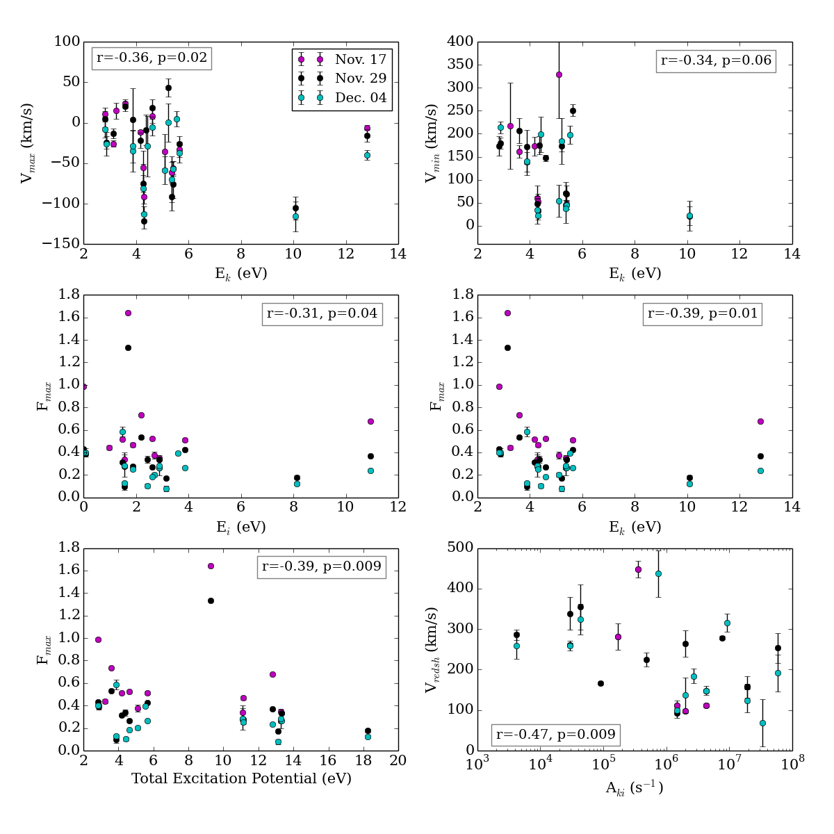
Figure 17: Marginal correlations observed between the velocity data and different atomic parameters. See text for details.

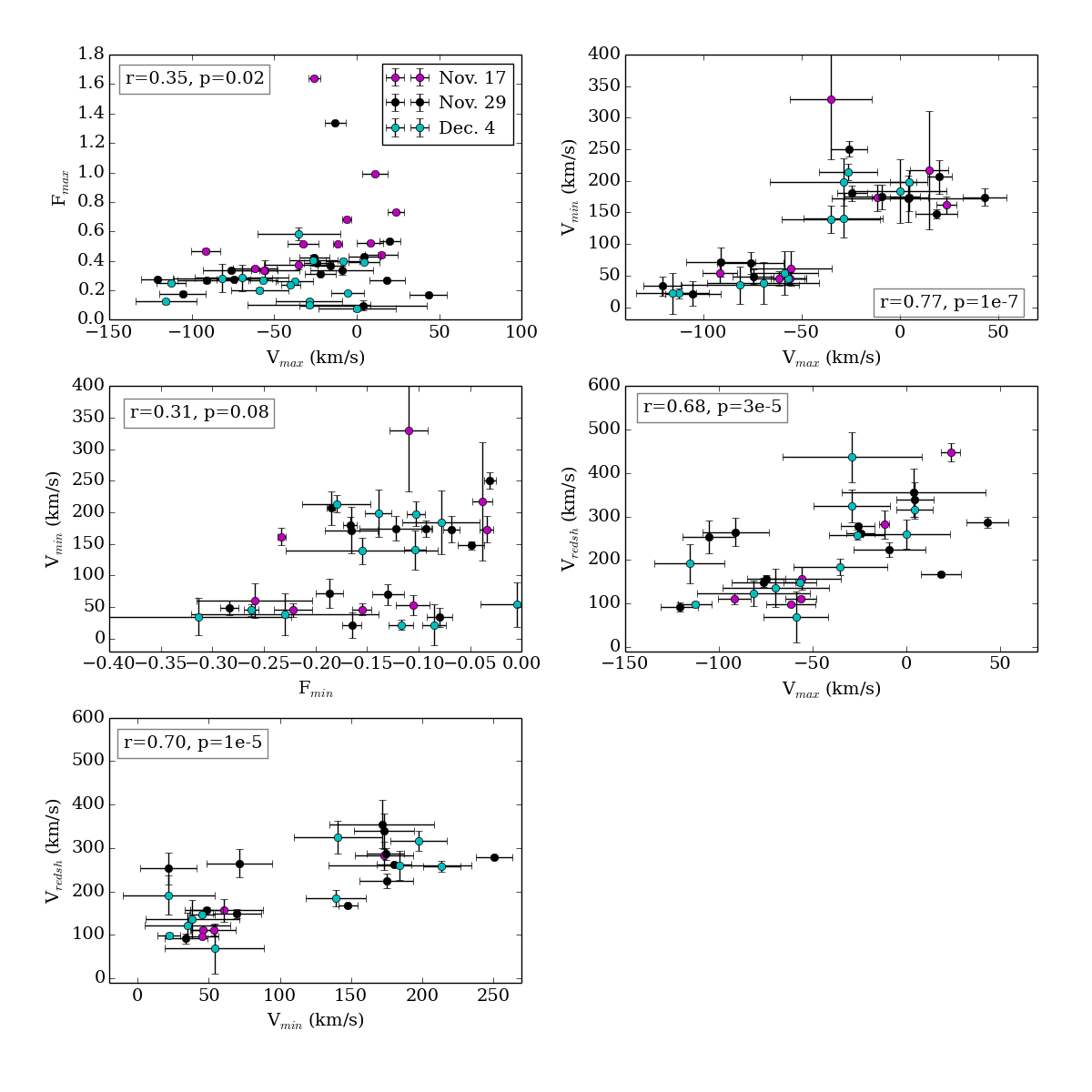
Figure 18: Correlations between the different line parameters. We note that the correlations between the peak, minimum, and maximum red-shifted velocities simply indicate that the lines are usually globally shifted.

Figure 17 displays the marginal correlations observed between the line parameters and the upper and lower energy of the levels (E_k and E_i) and the sum of the ionization and excitation potential. Figure 18 shows the correlations between the line parameters themselves, some of which are trivial, such as the correlation between all the different line velocities, which indicate that the lines tend to be globally shifted.

References

- Ábrahám et al. (2004) Ábrahám, P., Kóspál, Á., Csizmadia, S., et al. 2004, A&A, 428, 89
- Ábrahám et al. (2009) Ábrahám, P., Juhász, A., Dullemond, C.P., Kóspál, A.,van Boekel, R., Henning, Th., Moór, A., Mosoni, L., Sicilia-Aguilar, A., Sipos, N., 2009, Nature 459, 224
- Alcalá et al. (2014) Alcalá, J. M., Natta, A., Manara, C. F., et al. 2014, A&A, 561, AA2
- Alencar et al. (2001) Alencar, S., Johns-Krull, C., Basri, G., 2001, AJ 122, 3335
- Alencar et al. (2010) Alencar, S.H.P., Teixeira, P.S., Guimaraes, M.M., et al. 2010, A&A, 519, A88
- Alencar et al. (2012) Alencar, S. H. P., Bouvier, J., Walter, F. M., et al. 2012, A&A, 541, A116
- Appenzeller et al. (1986) Appenzeller, I., Jankovics, I., Jetter, R., 1986, A&ASS 64, 65
- Aspin (2011) Aspin, C. 2011, AJ, 142, 135
- Audard et al. (2010) Audard, M., Stringfellow, G. S., Güdel, M., et al. 2010, A&A, 511, A63
- Audard et al. (2014) Audard, M.; Abrahám, P.; Dunham, M.M. et al. Episodic Accretion in Young Stars. Protostars and Planets VI, 2014, 387
- Banzatti et al. (2015) Banzatti, A., Pontoppidan, K. M., Bruderer, S., Muzerolle, J., & Meyer, M. R. 2015, ApJ, 798, LL16
- Barron et al. (2008) Barron, J. T., Stumm, C., Hogg, D. W., Lang, D., & Roweis, S. 2008, AJ, 135, 414-422
- Beristain et al. (1998) Beristain, G., Edwards, S., & Kwan, J. 1998, ApJ, 499, 828
- Bertout et al. (1982) Bertout, C., Wolf, B., Carrasco, L., & Mundt, R. 1982, A&AS, 47, 419
- Bohlin et al. (1978) Bohlin, R. C., Savage, B. D., & Drake, J. F. 1978, ApJ, 224, 132
- Bonnefoy et al. (2016) Bonnefoy, M., Chauvin, G., Dougados, C., et al. 2016, arXiv:1608.08035
- Bouvier et al. (2003) Bouvier, J., Grankin, K. N., Alencar, S. H. P., et al. 2003, ApJ, 409, 169
- Bouvier et al. (2013) Bouvier, J., Grankin, K., Ellerbroek, L. E., Bouy, H., & Barrado, D. 2013, A&A, 557, A77
- Bouvier et al. (2014) Bouvier, J., Matt, S. P., Mohanty, S., et al. 2014, Protostars and Planets VI, 433
- Bozhinova et al. (2016) Bozhinova, I., Scholz, A., & Eislöffel, J. 2016, MNRAS, 458, 3118
- Bozhinova et al. (2016) Bozhinova, I., Scholz, A., Costigan, G., et al. 2016, MNRAS, 463, 4459
- Briceño et al. (2004) Briceño, C., Vivas, A. K., Hernández, J., et al. 2004, ApJ, 606, L123
- Brown et al. (2013) Brown, T. M., Baliber, N., Bianco, F. B., et al. 2013, PASP, 125, 1031
- Buysschaert et al. (2017) Buysschaert, B., Neiner, C., Richardson, N. D., et al. 2017, arXiv:1704.00576
- Calvet & Gullbring (1998) Calvet, N., & Gullbring, E. 1998, ApJ, 509, 802
- Caratti o Garatti et al. (2011) Caratti o Garatti, A., Garcia Lopez, R., Scholz, A., et al. 2011, A&A, 526, L1
- Cardelli et al. (1989) Cardelli, J., Clayton, G., Mathis, J., 1989, ApJ, 345, 245
- Chambers et al. (2016) Chambers, K. C., Magnier, E. A., Metcalfe, N., et al. 2016, arXiv:1612.05560
- Contreras Peña et al. (2014) Contreras Peña, C., Lucas, P. W., Froebrich, D., et al. 2014, MNRAS, 439, 1829
- Contreras Peña et al. (2017) Contreras Peña, C., Lucas, P. W., Kurtev, R., et al. 2017, MNRAS, 465, 3039
- Costigan et al. (2012) Costigan, G., Scholz, A., Stelzer, B., et al. 2012, MNRAS, 427, 1344
- Costigan et al. (2014) Costigan, G., Vink, J. S., Scholz, A., Ray, T., & Testi, L. 2014, MNRAS, 440, 3444
- Curcio et al. (1964) Curcio, J., Drummeler, L., Knestrick,G., 1964, Applied Optics Vol. 3, N. 12, 1401
- Cutri et al. (2003) Cutri R.M., Skrutskie, M.F., van Dyk, S. & 25 more coauthors, 2003yCat.2246, 0C, VizieR On-line Data Catalog: II/246
- Davis et al. (2015) Davis, A. B., Shappee, B. J., Archer Shappee, B., & ASAS-SN 2015, American Astronomical Society Meeting Abstracts, 225, 344.02
- Doi et al. (2010) Doi, M., Tanaka, M., Fukugita, M., et al. 2010, AJ, 139, 1628
- Dunham & Vorobyov (2012) Dunham, M. M., & Vorobyov, E. I. 2012, ApJ, 747, 52
- Eiroa et al. (2002) Eiroa, C., Oudmaijer, R.D., Davies, J.K. et al. 2002, A&A, 384, 1038
- Fang et al. (2009) Fang, M., van Boekel, R., Wang, W., Carmona, A., Sicilia-Aguilar, A., & Henning, T. 2009, A&A, 504, 461
- Fang et al. (2017) Fang, M., Kim, J. S., Pascucci, I., et al. 2017, AJ, 153, 188
- Fedele et al. (2007) Fedele, D., van den Ancker, M. E., Petr-Gotzens, M. G., & Rafanelli, P. 2007, A&A, 472, 207
- Flewelling et al. (2016) Flewelling, H. A., Magnier, E. A., Chambers, K. C., et al. 2016, arXiv:1612.05243
- Fukugita et al. (1996) Fukugita, M., Ichikawa, T., Gunn, J. E., et al. 1996, AJ, 111, 1748
- Gaia Collaboration et al. (2016) Gaia Collaboration, Prusti, T., de Bruijne, J. H. J., et al. 2016, A&A, 595, A1
- Gaia Collaboration et al. (2016) Gaia Collaboration, Brown, A. G. A., Vallenari, A., et al. 2016, A&A, 595, A2
- Gandolfi et al. (2008) Gandolfi, D., Alcalá, J.M., Leccia, S., et al. 2008, A&A 687, 1303
- Giannini et al. (2017) Giannini, T., Antoniucci, S., Lorenzetti, D., et al. 2017, arXiv:1704.05777
- Green et al. (2015) Green, G. M., Schlafly, E. F., Finkbeiner, D. P., et al. 2015, ApJ, 810, 25
- Gregory et al. (2014) Gregory, S. G., Holzwarth, V. R., Donati, J.-F., et al. 2014, IAU Symposium, 302, 44
- Grinin & Mitskevich (1988) Grinin, V. P., & Mitskevich, A. S. 1988, Bul- letin of the Crimean Astrophysical Observatory, Vol 78, 28
- Grinin et al. (1991) Grinin, V. P., Kiselev, N. N., Chernova, G. P., Minikulov, N. K., & Voshchinnikov, N. V. 1991, Ap&SS, 186, 283
- Gullbring et al. (1998) Gullbring, E., Hartmann, L., Briceño, C., Calvet, N., 1998, ApJ 492, 323
- Gunn et al. (2006) Gunn, J. E., Siegmund, W. A., Mannery, E. J., et al. 2006, AJ, 131, 2332
- Hamaguchi et al. (2012) Hamaguchi, K., Grosso, N., Kastner, J. H., et al. 2012, ApJ, 754, 32
- Hamann & Persson (1992) Hamann, F., & Persson, S.E., 1992, ApJS82, 247
- Hamann (1994) Hamann, F. , 1994, ApJS, 93, 485
- Hartmann & Kenyon (1996) Hartmann, L., & Kenyon, S., 1996, ARA&A, 34, 207
- Hartmann et al. (2001) Hartmann, L., Ballesteros-Paredes, J., Bergin, E., 2001, ApJ 562, 852
- Henden & Munari (2014) Henden, A., & Munari, U. 2014, Contributions of the Astronomical Observatory Skalnate Pleso, 43, 518
- Henderson & Stassun (2012) Henderson, C. B., & Stassun, K. G. 2012, ApJ, 747, 51
- Herbig (1950) Herbig, G., 1950, PASP, 62, 211
- Herbig (1977) Herbig, G., 1977, ApJ, 214, 747
- Herbig (1989) Herbig, G. H. 1989, European Southern Observatory Conference and Workshop Proceedings, 33, 233
- Herbig et al. (2001) Herbig, G., Aspin, C., Gilmore, A., Imhoff, C., Jones, A., 2001, PASP, 113, 1547
- Herbig et al. (2003) Herbig, G., Petrov, P., Duemmler, R., 2003, ApJ, 595, 384
- Herbig (2007) Herbig, G., 2007, AJ, 133, 2679
- Herbig (2008) Herbig, G., 2008, AJ, 135, 637
- Herbst et al. (1994) Herbst, W., Herbst, D., Grossman, E., Weinstein, D., 1994, AJ 108, 1906
- Herbst et al. (2002) Herbst, W., Bailer-Jones, C. A. L., Mundt, R., Meisenheimer, K., & Wackermann, R. 2002, A&A, 396, 513
- Herczeg et al. (2016) Herczeg, G. J., Dong, S., Shappee, B. J., et al. 2016, ApJ, 831, 133
- Holoien et al. (2014) Holoien, T. W.-S., Prieto, J. L., Stanek, K. Z., et al. 2014, ApJ, 785, LL35
- Horne & Baliunas (1986) Horne, J. H., & Baliunas, S. L. 1986, ApJ, 302, 757
- Jeffries (2007) Jeffries, R. D. 2007, MNRAS, 376, 1109
- Joy (1945) Joy, A. H. 1945, ApJ, 102, 168
- Juhász et al. (2012) Juhász, A., Dullemond, C. P., van Boekel, R., et al. 2012, ApJ, 744, 118
- Kaufer et al. (1999) Kaufer, A., Stahl, O., Tubbesing, S., et al. 1999, The Messenger, 95, 8
- Kaufer et al. (2000) Kaufer, A., Stahl, O., Tubbesing, S., et al. 2000, Proc. SPIE, 4008, 459
- Kenyon & Hartmann (1995) Kenyon, S.J. & Hartmann, L., 1995, ApJS , 101, 117
- Kóspál et al. (2008) Kóspál, Á., Nemeth, P., Abraham, P., et al. 2008, Information Bulletin on Variable Stars, 5819, 1
- Kóspál et al. (2011) Kóspál, Á., Ábrahám, P., Goto, M., et al. 2011, ApJ, 736, 72
- Kóspál et al. (2012) Kóspál, Á., Ábrahám, P., Acosta-Pulido, J. A., et al. 2012, ApJS, 201, 11
- Kóspál et al. (2014) Kóspál, Á., Mohler-Fischer, M., Sicilia-Aguilar, A., et al. 2014, A&A, 561, A61
- Kounkel et al. (2017) Kounkel, M., Hartmann, L., Loinard, L., et al. 2017, ApJ, 834, 142
- Kurosawa & Romanova (2013) Kurosawa, R., & Romanova, M. M. 2013, MNRAS, 431, 2673
- Lamm et al. (2005) Lamm, M. H., Mundt, R., Bailer-Jones, C. A. L., & Herbst, W. 2005, A&A, 430, 1005
- Lima et al. (2010) Lima, G. H. R. A., Alencar, S. H. P., Calvet, N., Hartmann, L., & Muzerolle, J. 2010, A&A, 522, A104
- Littlefair et al. (2010) Littlefair, S. P., Naylor, T., Mayne, N. J., Saunders, E. S., & Jeffries, R. D. 2010, MNRAS, 403, 545
- Lorenzetti et al. (2012) Lorenzetti, D., Antoniucci, S., Giannini, T., et al. 2012, ApJ, 749, 188
- Manara et al. (2017) Manara, C. F., Testi, L., Herczeg, G. J., et al. 2017, arXiv:1704.02842
- Martini et al. (2011) Martini, P., Stoll, R., Derwent, M. A., et al. 2011, PASP, 123, 187
- McNeil et al. (2004) McNeil, J. W., Reipurth, B., & Meech, K. 2004, IAU Circ., 8284, 1
- Mihalas (1978) Mihalas, D., 1978, “Stellar Atmospheres”, Ed. W.H. Freeman and Company, San Francisco
- Morin et al. (2010) Morin, J., Donati, J.-F., Petit, P., et al. 2010, MNRAS, 407, 2269
- Mortier & Collier Cameron (2017) Mortier, A., & Collier Cameron, A. 2017, arXiv:1702.03885
- Müller et al. (2013) Müller, A., Roccatagliata, V., Henning, T., et al. 2013, A&A, 556, AA3
- Muzerolle et al. (2001) Muzerolle, J., Calvet, N. & Hartmann, L., 2001, ApJ, 550, 944
- Natta et al. (1999) Natta, A., Prusti, T., Neri, R., et al. 1999, A&A, 350, 541
- Nisini et al. (2005) Nisini, B.; Antoniucci, S.; Giannini, T.; Lorenzetti, D., 2005, A&A, 429, 543
- Petrov et al. (2014) Petrov, P. P., Gahm, G. F., Herczeg, G. J., Stempels, H. C., & Walter, F. M. 2014, A&A, 568, LL10
- Principe et al. (2016) Principe, D. A., Sacco, G., Kastner, J. H., Stelzer, B., & Alcalá, J. M. 2016, MNRAS, 459, 2097
- Ralchenko et al. (2010) Ralchenko, Yu., Kramida, A.E., Reader, J., and NIST ASD Team (2010). NIST Atomic Spectra Database (ver. 4.0.1). Available: http://physics.nist.gov/asd. National Institute of Standards and Technology, Gaithersburg, MD.
- Reid et al. (2009) Reid, M. J., Menten, K. M., Zheng, X. W., et al. 2009, ApJ, 700, 137-148
- Saha (1921) Saha, M. N. 1921, Proceedings of the Royal Society of London Series A, 99, 135
- Scargle (1982) Scargle, J. D. 1982, ApJ, 263, 835
- Scholz et al. (2009) Scholz, A., Xu, X., Jayawardhana, R., et al. 2009, MNRAS, 398, 873
- Scholz (2013) Scholz, A. 2013, Mem. Soc. Astron. Italiana, 84, 890
- Shappee et al. (2014) Shappee, B., Prieto, J., Stanek, K. Z., et al. 2014, American Astronomical Society Meeting Abstracts #223, 223, 236.03
- Shappee et al. (2014) Shappee, B. J., Prieto, J. L., Grupe, D., et al. 2014, ApJ, 788, 48
- Shine & Linsky (1974) Shine, R. A., & Linsky, J. L. 1974, Sol. Phys., 39, 49
- Shu et al. (1994) Shu, F., Najita, J., Ostriker, E., et al. 1994, ApJ, 429, 781
- Sicilia-Aguilar et al. (2005) Sicilia-Aguilar, A., Hartmann, L., Szentgyorgyi, A., et al. 2005, AJ, 129, 363
- Sicilia-Aguilar et al. (2008) Sicilia-Aguilar, A., Merín, B., Hormuth, F., et al. 2008, ApJ, 673, 382-399
- Sicilia-Aguilar et al. (2010) Sicilia-Aguilar, A., Henning, Th., Hartmann, L., 2010, ApJ, 710, 597
- Sicilia-Aguilar et al. (2012) Sicilia-Aguilar, A., Kóspál, Á., Setiawan, J., et al. 2012, A&A, 544, A93
- Sicilia-Aguilar et al. (2015) Sicilia-Aguilar, A., Fang, M., Roccatagliata, V., et al. 2015, A&A, 580, A82
- Siess et al. (2000) Siess, L., Dufour, E. & Forestini, M. 2000 A&A , 358, 593
- Siwak et al. (2013) Siwak, M., Rucinski, S. M., Matthews, J. M., et al. 2013, MNRAS, 432, 194
- Stoughton et al. (2002) Stoughton, C., Lupton, R. H., Bernardi, M., et al. 2002, AJ, 123, 485
- Tokovinin et al. (2013) Tokovinin, A., Fischer, D. A., Bonati, M., et al. 2013, PASP, 125, 1336
- Yuan et al. (2013) Yuan, H. B., Liu, X. W., & Xiang, M. S. 2013, MNRAS, 430, 2188
- Zechmeister & Kuerster (2009) Zechmeister, M., Kuerster, M. 2009, A&A, 496, 577