Chiral damping, chiral gyromagnetism and current-induced torques in textured one-dimensional Rashba ferromagnets

Abstract

We investigate Gilbert damping, spectroscopic gyromagnetic ratio and current-induced torques in the one-dimensional Rashba model with an additional noncollinear magnetic exchange field. We find that the Gilbert damping differs between left-handed and right-handed Néel-type magnetic domain walls due to the combination of spatial inversion asymmetry and spin-orbit interaction (SOI), consistent with recent experimental observations of chiral damping. Additionally, we find that also the spectroscopic $g$ factor differs between left-handed and right-handed Néel-type domain walls, which we call chiral gyromagnetism. We also investigate the gyromagnetic ratio in the Rashba model with collinear magnetization, where we find that scattering corrections to the $g$ factor vanish for zero SOI, become important for finite spin-orbit coupling, and tend to stabilize the gyromagnetic ratio close to its nonrelativistic value.

I Introduction

In magnetic bilayer systems with structural inversion asymmetry the energies of left-handed and right-handed Néel-type domain walls differ due to the Dzyaloshinskii-Moriya interaction (DMI) Moriya (1960); Dzyaloshinsky (1958); Heide et al. (2008); Ferriani et al. (2008). DMI is a chiral interaction, i.e., it distinguishes between left-handed and right-handed spin-spirals. Not only the energy is sensitive to the chirality of spin-spirals. Recently, it has been reported that the orbital magnetic moments differ as well between left-handed and right-handed cycloidal spin spirals in magnetic bilayers Yamamoto et al. (2017); Lux et al. (2017). Moreover, the experimental observation of asymmetry in the velocity of domain walls driven by magnetic fields suggests that also the Gilbert damping is sensitive to chirality Jué et al. (2015); Akosa et al. (2016).

In this work we show that additionally the spectroscopic gyromagnetic ratio $\gamma$ is sensitive to the chirality of spin-spirals. The spectroscopic gyromagnetic ratio $\gamma$ can be defined by the equation

$$\frac{{\rm d}{\bm{m}}}{{\rm d}t}=\gamma{\bm{T}},$$ (1)

where ${\bm{T}}$ is the torque that acts on the magnetic moment ${\bm{m}}$ and ${\rm d}{\bm{m}}/{\rm d}t$ is the resulting rate of change. $\gamma$ enters the Landau-Lifshitz-Gilbert equation (LLG):

$$\frac{{\rm d}\hat{{\bm{M}}}}{{\rm d}t}=\gamma\hat{{\bm{M}}}\times{\bm{H}}^{\rm eff}+{\bm{\alpha}}^{\rm G}\hat{{\bm{M}}}\times\frac{{\rm d}\hat{{\bm{M}}}}{{\rm d}t},$$ (2)

where $\hat{{\bm{M}}}$ is a normalized vector that points in the direction of the magnetization and the tensor ${\bm{\alpha}}^{\rm G}$ describes the Gilbert damping. The chirality of the gyromagnetic ratio provides another mechanism for asymmetries in domain-wall motion between left-handed and right-handed domain walls.

Not only the damping and the gyromagnetic ratio exhibit chiral corrections in inversion asymmetric systems but also the current-induced torques. Among these torques that act on domain-walls are the adiabatic and nonadiabatic spin-transfer torques Tserkovnyak et al. (2006); Gilmore et al. (2011); Garate et al. (2009); Kim et al. (2015a) and the spin-orbit torque Khvalkovskiy et al. (2013); van der Bijl and Duine (2012); Freimuth et al. (2014a); Freimuth et al. (2015). Based on phenomenological grounds additional types of torques have been suggested Hals and Brataas (2013). Since this large number of contributions are difficult to disentangle experimentally, current-driven domain-wall motion in inversion asymmetric systems is not yet fully understood.

The two-dimensional Rashba model with an additional exchange splitting has been used to study spintronics effects associated with the interfaces in magnetic bilayer systems Manchon and Zhang (2008); Manchon et al. (2015); Pesin and MacDonald (2012); Qaiumzadeh et al. (2015); Ado et al. (2017). Recently, interest in the role of DMI in one-dimensional magnetic chains has been triggered Kashid et al. (2014); Schweflinghaus et al. (2016). For example, the magnetic moments in bi-atomic Fe chains on the Ir surface order in a 120^∘ spin-spiral state due to DMI Menzel et al. (2012). Apart from DMI, also other chiral effects, such as chiral damping and chiral gyromagnetism, are expected to be important in one-dimensional magnetic chains on heavy metal substrates. The one-dimensional Rashba model Barke et al. (2006); Okuda et al. (2010) with an additional exchange splitting can be used to simulate spin-orbit driven effects in one-dimensional magnetic wires on substrates Shick et al. (2005); Komelj et al. (2006); Gambardella et al. (2004). While the generalized Bloch theorem Sandratskii (1986) usually cannot be used to treat spin-spirals when SOI is included in the calculation, the one-dimensional Rashba model has the advantage that it can be solved with the help of the generalized Bloch theorem, or with a gauge-field approach Fujita et al. (2011), when the spin-spiral is of Néel-type. When the generalized Bloch theorem cannot be employed one needs to resort to a supercell approach Yang et al. (2015), use open boundary conditions Yuan and Kelly (2016); Yuan et al. (2014), or apply perturbation theory Lux et al. (2017); Freimuth et al. (2013); Freimuth et al. (2014b); Tserkovnyak et al. (2006); Freimuth et al. (2017); Kohno et al. (2016) in order to study spintronics effects in noncollinear magnets with SOI. In the case of the one-dimensional Rashba model the DMI and the exchange parameters were calculated both directly based on a gauge-field approach and from perturbation theory Freimuth et al. (2017). The results from the two approaches were found to be in perfect agreement. Thus, the one-dimensional Rashba model provides also an excellent opportunity to verify expressions obtained from perturbation theory by comparison to the results from the generalized Bloch theorem or from the gauge-field approach.

In this work we study chiral gyromagnetism and chiral damping in the one-dimensional Rashba model with an additional noncollinear magnetic exchange field. The one-dimensional Rashba model is very well suited to study these SOI-driven chiral spintronics effects, because it can be solved in a very transparent way without the need for a supercell approach, open boundary conditions or perturbation theory. We describe scattering effects by the Gaussian scalar disorder model. To investigate the role of disorder for the gyromagnetic ratio in general, we study $\gamma$ also in the two-dimensional Rashba model with collinear magnetization. Additionally, we compute the current-induced torques in the one-dimensional Rashba model.

This paper is structured as follows: In section II.1 we introduce the one-dimensional Rashba model. In section II.2 we discuss the formalism for the calculation of the Gilbert damping and of the gyromagnetic ratio. In section II.3 we present the formalism used to calculate the current-induced torques. In sections III.1, III.2, and III.3 we discuss the gyromagnetic ratio, the Gilbert damping, and the current-induced torques in the one-dimensional Rashba model, respectively. This paper ends with a summary in section IV.

II Formalism

II.1 One-dimensional Rashba model

The two-dimensional Rashba model is given by the Hamiltonian Manchon et al. (2015)

$$H =-\frac{\hbar^{2}}{2m_{e}}\frac{\partial^{2}}{\partial x^{2}}-\frac{\hbar^{2}}{2m_{e}}\frac{\partial^{2}}{\partial y^{2}}+$$ (3)

$$+i\alpha^{\rm R}\sigma_{y}\frac{\partial}{\partial x}-i\alpha^{\rm R}\sigma_{x}\frac{\partial}{\partial y}+\frac{\Delta V}{2}{\bm{\sigma}}\cdot\hat{{\bm{M}}}({\bm{r}}),$$

where the first line describes the kinetic energy, the first two terms in the second line describe the Rashba SOI and the last term in the second line describes the exchange splitting. $\hat{{\bm{M}}}({\bm{r}})$ is the magnetization direction, which may depend on the position ${\bm{r}}=(x,y)$, and ${\bm{\sigma}}$ is the vector of Pauli spin matrices. By removing the terms with the $y$-derivatives from Eq. (3), i.e., $-\frac{\hbar^{2}}{2m_{e}}\frac{\partial^{2}}{\partial y^{2}}$ and $-i\alpha^{\rm R}\sigma_{x}\frac{\partial}{\partial y}$, one obtains a one-dimensional variant of the Rashba model with the Hamiltonian Freimuth et al. (2017)

$$H=-\frac{\hbar^{2}}{2m_{e}}\frac{\partial^{2}}{\partial x^{2}}+i\alpha^{\rm R}\sigma_{y}\frac{\partial}{\partial x}+\frac{\Delta V}{2}{\bm{\sigma}}\cdot\hat{{\bm{M}}}(x).$$ (4)

Eq. (4) is invariant under the simultaneous rotation of ${\bm{\sigma}}$ and of the magnetization $\hat{{\bm{M}}}$ around the $y$ axis. Therefore, if $\hat{{\bm{M}}}(x)$ describes a flat cycloidal spin-spiral propagating into the $x$ direction, as given by

$$\hat{{\bm{M}}}(x)=\begin{pmatrix}\sin(qx)\\ 0\\ \cos(qx)\end{pmatrix},\\$$ (5)

we can use the unitary transformation

$$\mathcal{U}(x)=\left(\begin{array}[]{cc}\cos(\frac{qx}{2})&-\sin(\frac{qx}{2})\\[6.0pt] \sin(\frac{qx}{2})&\cos(\frac{qx}{2})\end{array}\right)$$ (6)

in order to transform Eq. (4) into a position-independent effective Hamiltonian Freimuth et al. (2017):

$$H=\frac{1}{2m}\left(p_{x}+eA^{\rm eff}_{x}\right)^{2}-\frac{m(\alpha^{\rm R})^{2}}{2\hbar^{2}}+\frac{\Delta V}{2}\sigma_{z},$$ (7)

where $p_{x}=-i\hbar\partial/\partial x$ is the $x$ component of the momentum operator and

$$A^{\rm eff}_{x}=-\frac{m}{e\hbar}\left(\alpha^{\rm R}+\frac{\hbar^{2}}{2m}q\right)\sigma_{y}$$ (8)

is the $x$-component of the effective magnetic vector potential. Eq. (8) shows that the noncollinearity described by $q$ acts like an effective SOI in the special case of the one-dimensional Rashba model. This suggests to introduce the concept of effective SOI strength

$$\alpha_{\rm eff}^{\rm R}=\alpha^{\rm R}_{\phantom{e}}+\frac{\hbar^{2}}{2m}q.$$ (9)

Based on this concept of the effective SOI strength one can obtain the $q$-dependence of the one-dimensional Rashba model from its $\alpha^{\rm R}$-dependence at $q=0$. That a noncollinear magnetic texture provides a nonrelativistic effective SOI has been found also in the context of the intrinsic contribution to the nonadiabatic torque in the absence of relativistic SOI, which can be interpreted as a spin-orbit torque arising from this effective SOI Kim et al. (2015b). While the Hamiltonian in Eq. (4) depends on position $x$ through the position-dependence of the magnetization $\hat{{\bm{M}}}(x)$ in Eq. (5), the effective Hamiltonian in Eq. (7) is not dependent on $x$ and therefore easy to diagonalize.

II.2 Gilbert damping and gyromagnetic ratio

In collinear magnets damping and gyromagnetic ratio can be extracted from the tensor Freimuth et al. (2015)

$$\Lambda_{ij}=-\frac{1}{V}\!\lim_{\omega\to 0}\!\frac{{\rm Im}G_{\mathcal{T}_{i},\mathcal{T}_{j}}^{\rm R}(\hbar\omega)}{\hbar\omega},$$ (10)

where $V$ is the volume of the unit cell and

$$G_{\mathcal{T}_{i},\mathcal{T}_{j}}^{\rm R}(\hbar\omega)=-i\int\limits_{0}^{\infty}{\rm d}te^{i\omega t}\left\langle[\mathcal{T}_{i}(t),\mathcal{T}_{j}(0)]_{-}\right\rangle$$ (11)

is the retarded torque-torque correlation function. $\mathcal{T}_{i}$ is the $i$-th component of the torque operator Freimuth et al. (2015). The dc-limit $\omega\rightarrow 0$ in Eq. (10) is only justified when the frequency of the magnetization dynamics, e.g., the ferromagnetic resonance frequency, is smaller than the relaxation rate of the electronic states. In thin magnetic layers and monoatomic chains on substrates this is typically the case due to the strong interfacial disorder. However, in very pure crystalline samples at low temperatures the relaxation rate may be smaller than the ferromagnetic resonance frequency and one needs to assume $\omega>0$ in Eq. (10) Edwards (2016); Costa and Muniz (2015). The tensor ${\bm{\Lambda}}$ depends on the magnetization direction $\hat{{\bm{M}}}$ and we decompose it into the tensor ${\bm{S}}$, which is even under magnetization reversal (${\bm{S}}(\hat{{\bm{M}}})={\bm{S}}(-\hat{{\bm{M}}})$), and the tensor ${\bm{A}}$, which is odd under magnetization reversal (${\bm{A}}(\hat{{\bm{M}}})=-{\bm{A}}(-\hat{{\bm{M}}})$), such that ${\bm{\Lambda}}={\bm{S}}+{\bm{A}}$, where

$$S_{ij}(\hat{{\bm{M}}})=\frac{1}{2}\left[\Lambda_{ij}(\hat{{\bm{M}}})+\Lambda_{ij}(-\hat{{\bm{M}}})\right]$$ (12)

and

$$A_{ij}(\hat{{\bm{M}}})=\frac{1}{2}\left[\Lambda_{ij}(\hat{{\bm{M}}})-\Lambda_{ij}(-\hat{{\bm{M}}})\right].$$ (13)

One can show that ${\bm{S}}$ is symmetric, i.e., $S_{ij}(\hat{{\bm{M}}})=S_{ji}(\hat{{\bm{M}}})$, while ${\bm{A}}$ is antisymmetric, i.e., $A_{ij}(\hat{{\bm{M}}})=-A_{ji}(\hat{{\bm{M}}})$.

The Gilbert damping may be extracted from the symmetric component $S$ as follows Freimuth et al. (2015):

$$\alpha^{\rm G}_{ij}=\frac{|\gamma|S^{\phantom{e}}_{ij}}{M\mu_{0}},$$ (14)

where $M$ is the magnetization. The gyromagnetic ratio $\gamma$ is obtained from $\Lambda$ according to the equation Freimuth et al. (2015)

$$\frac{1}{\gamma}=\frac{1}{2\mu_{0}M}\sum_{ijk}\epsilon_{ijk}\Lambda_{ij}\hat{M}_{k}=\frac{1}{2\mu_{0}M}\sum_{ijk}\epsilon_{ijk}A_{ij}\hat{M}_{k}.$$ (15)

It is convenient to discuss the gyromagnetic ratio in terms of the dimensionless $g$-factor, which is related to $\gamma$ through $\gamma=g\mu_{0}\mu_{\rm B}/\hbar$. Consequently, the $g$-factor is given by

$$\frac{1}{g}=\frac{\mu_{\rm B}}{2\hbar M}\sum_{ijk}\epsilon_{ijk}\Lambda_{ij}\hat{M}_{k}=\frac{\mu_{\rm B}}{2\hbar M}\sum_{ijk}\epsilon_{ijk}A_{ij}\hat{M}_{k}.$$ (16)

Due to the presence of the Levi-Civita tensor $\epsilon_{ijk}$ in Eq. (15) and in Eq. (16) the gyromagnetic ratio and the $g$-factor are determined solely by the antisymmetric component ${\bm{A}}$ of ${\bm{\Lambda}}$.

Various different conventions are used in the literature concerning the sign of the $g$-factor Brown et al. (2000). Here, we define the sign of the $g$-factor such that $\gamma>0$ for $g>0$ and $\gamma<0$ for $g<0$. According to Eq. (1) the rate of change of the magnetic moment is therefore parallel to the torque for positive $g$ and antiparallel to the torque for negative $g$. While we are interested in this work in the spectroscopic $g$-factor, and hence in the relation between the rate of change of the magnetic moment and the torque, Ref. Brown et al. (2000) discusses the relation between the magnetic moment ${\bm{m}}$ and the angular momentum ${\bm{L}}$ that generates it, i.e., ${\bm{m}}=\gamma_{\rm static}{\bm{L}}$. Since differentiation with respect to time and use of ${\bm{T}}={\rm d}{\bm{L}}/{\rm d}t$ leads to Eq. (1) our definition of the signs of $g$ and $\gamma$ agrees essentially with the one suggested in Ref. Brown et al. (2000), which proposes to use a positive $g$ when the magnetic moment is parallel to the angular momentum generating it and a negative $g$ when the magnetic moment is antiparallel to the angular momentum generating it.

Combining Eq. (14) and Eq. (15) we can express the Gilbert damping in terms of ${\bm{A}}$ and ${\bm{S}}$ as follows:

$$\alpha^{\rm G}_{xx}=\frac{S_{xx}}{|A_{xy}|}.$$ (17)

In the independent particle approximation Eq. (10) can be written as ${\Lambda}^{\phantom{I}}_{ij}={\Lambda}^{\rm I(a)}_{ij}+{\Lambda}^{\rm I(b)}_{ij}+{\Lambda}^{\rm II}_{ij}$, where

Here, $d$ is the dimension ($d=1$ or $d=2$ or $d=3$), $G^{\rm R}_{{\bm{k}}}(\mathcal{E})$ is the retarded Green’s function and $G^{\rm A}_{{\bm{k}}}(\mathcal{E})=[G^{\rm R}_{{\bm{k}}}(\mathcal{E})]^{\dagger}$. $\mathcal{E}_{\rm F}$ is the Fermi energy. ${\Lambda}^{\rm I(b)\phantom{I}}_{ij}$ is symmetric under the interchange of the indices $i$ and $j$ while ${\Lambda}^{\rm II}_{ij}$ is antisymmetric. The term ${\Lambda}^{\rm I(a)\phantom{I}}_{ij}$ contains both symmetric and antisymmetric components. Since the Gilbert damping tensor is symmetric, both ${\Lambda}^{\rm I(b)\phantom{I}}_{ij}$ and ${\Lambda}^{\rm I(a)\phantom{I}}_{ij}$ contribute to it. Since the gyromagnetic tensor is antisymmetric, both ${\Lambda}^{\rm II}_{ij}$ and ${\Lambda}^{\rm I(a)\phantom{I}}_{ij}$ contribute to it.

In order to account for disorder we use the Gaussian scalar disorder model, where the scattering potential $\mathcal{V}({\bm{r}})$ satisfies $\langle\mathcal{V}({\bm{r}})\rangle=0$ and $\langle\mathcal{V}({\bm{r}})\mathcal{V}({\bm{r}}^{\prime})\rangle=U\delta({\bm{r}}-{\bm{r}}^{\prime})$. This model is frequently used to calculate transport properties in disordered multiband model systems Kovalev et al. (2010), but it has also been combined with ab-initio electronic structure calculations to study the anomalous Hall effect Weischenberg et al. (2011); Czaja et al. (2014) and the anomalous Nernst effect Weischenberg et al. (2013) in transition metals and their alloys.

In the clean limit, i.e., in the limit $U\rightarrow 0$, the antisymmetric contribution to Eq. (II.2) can be written as $A^{\phantom{i}}_{ij}=A^{\rm int}_{ij}+A^{\rm scatt}_{ij}$, where the intrinsic part is given by

$$A^{\rm int}_{ij} =\hbar\int\!\!\frac{{\rm d}^{d}k}{(2\pi)^{d}}\sum_{n,m}[f_{{\bm{k}}n}-f_{{\bm{k}}m}]{\rm Im}\frac{\mathcal{T}^{i}_{{\bm{k}}nm}\mathcal{T}^{j}_{{\bm{k}}mn}}{(\mathcal{E}_{{\bm{k}}n}-\mathcal{E}_{{\bm{k}}m})^{2}}$$ (18)

$$=2\hbar\int\!\!\frac{{\rm d}^{d}k}{(2\pi)^{d}}\sum_{n}\sum_{ll^{\prime}}f_{{\bm{k}}n}{\rm Im}\left[\frac{\partial\langle u_{{\bm{k}}n}|}{\partial\hat{M}_{l}}\frac{\partial|u_{{\bm{k}}n}\rangle}{\partial\hat{M}_{l^{\prime}}}\right]\times$$

$$\quad\quad\times\sum_{mm^{\prime}}\epsilon_{ilm}\epsilon_{jl^{\prime}m^{\prime}}\hat{M}_{m}\hat{M}_{m^{\prime}}.$$

The second line in Eq. (18) expresses $A^{\rm int}_{ij}$ in terms of the Berry curvature in magnetization space Qian and Vignale (2002). The scattering contribution is given by

$$A^{\rm scatt}_{ij}=\hbar\sum_{nm}\int\!\!\frac{{\rm d}^{d}k}{(2\pi)^{d}}\delta(\mathcal{E}_{\rm F}-\mathcal{E}_{{\bm{k}}n}){\rm Im}\Biggl{\{}$$ (19)

$$- \left[\mathcal{M}^{i}_{{\bm{k}}nm}\frac{\gamma^{\phantom{i}}_{{\bm{k}}mn}}{\gamma^{\phantom{i}}_{{\bm{k}}nn}}\mathcal{T}^{j}_{{\bm{k}}nn}-\mathcal{M}^{j}_{{\bm{k}}nm}\frac{\gamma^{\phantom{i}}_{{\bm{k}}mn}}{\gamma^{\phantom{i}}_{{\bm{k}}nn}}\mathcal{T}^{i}_{{\bm{k}}nn}\right]$$

$$+ \left[\mathcal{M}^{i}_{{\bm{k}}mn}\tilde{\mathcal{T}}^{j}_{{\bm{k}}nm}-\mathcal{M}^{j}_{{\bm{k}}mn}\tilde{\mathcal{T}}^{i}_{{\bm{k}}nm}\right]$$

$$- \left[\mathcal{M}^{i}_{{\bm{k}}nm}\frac{\gamma^{\phantom{i}}_{{\bm{k}}mn}}{\gamma^{\phantom{i}}_{{\bm{k}}nn}}\tilde{\mathcal{T}}^{j}_{{\bm{k}}nn}-\mathcal{M}^{j}_{{\bm{k}}nm}\frac{\gamma^{\phantom{i}}_{{\bm{k}}mn}}{\gamma^{\phantom{i}}_{{\bm{k}}nn}}\tilde{\mathcal{T}}^{i}_{{\bm{k}}nn}\right]$$

$$+ \left[\tilde{\mathcal{T}}^{i}_{{\bm{k}}nn}\frac{\gamma^{\phantom{i}}_{{\bm{k}}nm}}{\gamma^{\phantom{i}}_{{\bm{k}}nn}}\frac{\tilde{\mathcal{T}}^{j}_{{\bm{k}}mn}}{\mathcal{E}_{{\bm{k}}n}-\mathcal{E}_{{\bm{k}}m}}-\tilde{\mathcal{T}}^{j}_{{\bm{k}}nn}\frac{\gamma^{\phantom{i}}_{{\bm{k}}nm}}{\gamma^{\phantom{i}}_{{\bm{k}}nn}}\frac{\tilde{\mathcal{T}}^{i}_{{\bm{k}}mn}}{\mathcal{E}_{{\bm{k}}n}-\mathcal{E}_{{\bm{k}}m}}\right]$$

$$+\frac{1}{2} \left[\tilde{\mathcal{T}}^{i}_{{\bm{k}}nm}\frac{1}{\mathcal{E}_{{\bm{k}}n}-\mathcal{E}_{{\bm{k}}m}}\tilde{\mathcal{T}}^{j}_{{\bm{k}}mn}-\tilde{\mathcal{T}}^{j}_{{\bm{k}}nm}\frac{1}{\mathcal{E}_{{\bm{k}}n}-\mathcal{E}_{{\bm{k}}m}}\tilde{\mathcal{T}}^{i}_{{\bm{k}}mn}\right]$$

$$+ \Bigl{[}\mathcal{T}^{j}_{{\bm{k}}nn}\frac{\gamma^{\phantom{i}}_{{\bm{k}}nm}}{\gamma^{\phantom{i}}_{{\bm{k}}nn}}\frac{1}{\mathcal{E}_{{\bm{k}}n}-\mathcal{E}_{{\bm{k}}m}}\tilde{\mathcal{T}}^{i}_{{\bm{k}}mn}$$

$$-\mathcal{T}^{i}_{{\bm{k}}nn}\frac{\gamma^{\phantom{i}}_{{\bm{k}}nm}}{\gamma^{\phantom{i}}_{{\bm{k}}nn}}\frac{1}{\mathcal{E}_{{\bm{k}}n}-\mathcal{E}_{{\bm{k}}m}}\tilde{\mathcal{T}}^{j}_{{\bm{k}}mn}\Bigr{]}\Biggr{\}}.$$

Here, $\mathcal{T}^{i}_{{\bm{k}}nm}=\langle u_{{\bm{k}}n}|\mathcal{T}_{i}{\phantom{i}}|u_{{\bm{k}}m}\rangle$ are the matrix elements of the torque operator. $\tilde{\mathcal{T}}^{i}_{{\bm{k}}nm}$ denotes the vertex corrections of the torque, which solve the equation

$$\tilde{\mathcal{T}}^{i}_{{\bm{k}}nm}= \sum_{p}\int\frac{{\rm d}^{n}k^{\prime}}{(2\pi)^{n-1}}\frac{\delta(\mathcal{E}_{F}-\mathcal{E}_{{\bm{k}}^{\prime}p})}{2\gamma^{\phantom{i}}_{{\bm{k}}^{\prime}pp}}\times$$ (20)

$$\times \langle u_{{\bm{k}}n}|u_{{\bm{k}}^{\prime}p}\rangle\left[\tilde{\mathcal{T}}^{i}_{{\bm{k}}^{\prime}pp}+\mathcal{T}^{i}_{{\bm{k}}^{\prime}pp}\right]\langle u_{{\bm{k}}^{\prime}p}|u_{{\bm{k}}m}\rangle.$$

The matrix $\gamma^{\phantom{i}}_{{\bm{k}}nm}$ is given by

$$\gamma^{\phantom{i}}_{{\bm{k}}nm}=-\pi\sum_{p}\int\!\!\frac{{\rm d}^{d}k^{\prime}}{(2\pi)^{d}}\delta(\mathcal{E}_{\rm F}-\mathcal{E}_{{\bm{k}}^{\prime}p})\langle u_{{\bm{k}}n}|u_{{\bm{k}}^{\prime}p}\rangle\langle u_{{\bm{k}}^{\prime}p}|u_{{\bm{k}}m}\rangle$$ (21)

and the Berry connection in magnetization space is defined as

$$i\mathcal{M}_{{\bm{k}}nm}^{j}=i\frac{\mathcal{T}_{{\bm{k}}nm}^{j}}{\mathcal{E}_{{\bm{k}}m}-\mathcal{E}_{{\bm{k}}n}}.$$ (22)

The scattering contribution Eq. (19) formally resembles the side-jump contribution to the AHE Kovalev et al. (2010) as obtained from the scalar disorder model: It can be obtained by replacing the velocity operators in Ref. Kovalev et al. (2010) by torque operators. We find that in collinear magnets without SOI this scattering contribution vanishes. The gyromagnetic ratio is then given purely by the intrinsic contribution Eq. (18). This is an interesting difference to the AHE: Without SOI all contributions to the AHE are zero in collinear magnets, while both the intrinsic and the side-jump contributions are generally nonzero in the presence of SOI.

In the absence of SOI Eq. (18) can be expressed in terms of the magnetization Qian and Vignale (2002):

$$A^{\rm int}_{ij}=-\frac{\hbar}{2\mu_{\rm B}}\sum_{k}\epsilon_{ijk}M_{k}.$$ (23)

Inserting Eq. (23) into Eq. (16) yields $g=-2$, i.e., the expected nonrelativistic value of the $g$-factor.

The $g$-factor in the presence of SOI is usually assumed to be given by Kittel (1949)

$$g=-2\frac{M_{\rm spin}+M_{\rm orb}}{M_{\rm spin}}=-2\frac{M}{M_{\rm spin}},$$ (24)

where $M_{\rm orb}$ is the orbital magnetization, $M_{\rm spin}$ is the spin magnetization and $M=M_{\rm orb}+M_{\rm spin}$ is the total magnetization. The $g$-factor obtained from Eq. (24) is usually in good agreement with experimental results Schoen et al. (2017). When SOI is absent, the orbital magnetization is zero, $M_{\rm orb}=0$, and consequently Eq. (24) yields $g=-2$ in that case. Eq. (16) can be rewritten as

$$\frac{1}{g} =\frac{M_{\rm spin}}{M}\frac{\mu_{\rm B}^{\phantom{B}}}{2\hbar M_{\rm spin}}\sum_{ijk}\epsilon_{ijk}A_{ij}\hat{M}_{k}=\frac{M_{\rm spin}}{M}\frac{1}{g_{1}^{\phantom{1}}},$$ (25)

with

$$\frac{1}{g_{1}^{\phantom{1}}}=\frac{\mu_{\rm B}^{\phantom{B}}}{2\hbar M_{\rm spin}}\sum_{ijk}\epsilon_{ijk}A_{ij}\hat{M}_{k}.$$ (26)

From the comparison of Eq. (25) with Eq. (24) it follows that Eq. (24) holds exactly if $g_{1}^{\phantom{1}}=-2$ is satisfied. However, Eq. (26) usually yields $g_{1}^{\phantom{1}}=-2$ only in collinear magnets when SOI is absent, otherwise $g_{1}^{\phantom{1}}\neq-2$. In the one-dimensional Rashba model the orbital magnetization is zero, $M_{\rm orb}=0$, and consequently

$$\frac{1}{g}=\frac{\mu_{\rm B}^{\phantom{B}}}{2\hbar M_{\rm spin}}\sum_{ijk}\epsilon_{ijk}A_{ij}\hat{M}_{k}.$$ (27)

The symmetric contribution can be written as $S^{\phantom{i}}_{ij}=S^{\rm int}_{ij}+S^{\rm RR-vert}_{ij}+S^{\rm RA-vert}_{ij}$, where

$$S^{\rm int}_{ij}=\frac{1}{h}\int\!\!\frac{{\rm d}^{d}k}{(2\pi)^{d}}{\rm Tr}\left\{\mathcal{T}_{i}G_{{\bm{k}}}^{\rm R}(\mathcal{E}_{\rm F})\mathcal{T}_{j}\left[G_{{\bm{k}}}^{\rm A}(\mathcal{E}_{\rm F})-G_{{\bm{k}}}^{\rm R}(\mathcal{E}_{\rm F})\right]\right\}$$ (28)

and

$$S^{\rm RR-vert}_{ij}=-\frac{1}{h}\int\!\!\frac{{\rm d}^{d}k}{(2\pi)^{d}}{\rm Tr}\left\{\tilde{\mathcal{T}}^{\rm RR}_{i}G_{{\bm{k}}}^{\rm R}(\mathcal{E}_{\rm F})\mathcal{T}^{\phantom{i}}_{j}G_{{\bm{k}}}^{\rm R}(\mathcal{E}_{\rm F})\right\}$$ (29)

and

$$S^{\rm AR-vert}_{ij}=\frac{1}{h}\int\!\!\frac{{\rm d}^{d}k}{(2\pi)^{d}}{\rm Tr}\left\{\tilde{\mathcal{T}}^{\rm AR}_{i}G_{{\bm{k}}}^{\rm R}(\mathcal{E}_{\rm F})\mathcal{T}^{\phantom{i}}_{j}G_{{\bm{k}}}^{\rm A}(\mathcal{E}_{\rm F})\right\},$$ (30)

where $G^{\rm R}_{{\bm{k}}}(\mathcal{E}_{\rm F})=\hbar[\mathcal{E}^{\phantom{i}}_{\rm F}-H^{\phantom{i}}_{{\bm{k}}}-\Sigma_{{\bm{k}}}^{\rm R}(\mathcal{E}_{\rm F})]^{-1}$ is the retarded Green’s function, $G_{{\bm{k}}}^{\rm A}(\mathcal{E}_{\rm F})=\left[G_{{\bm{k}}}^{\rm R}(\mathcal{E}_{\rm F})\right]^{\dagger}$ is the advanced Green’s function and

$$\Sigma^{\rm R}(\mathcal{E}_{\rm F})=\frac{U}{\hbar}\int\!\!\frac{{\rm d}^{d}k}{(2\pi)^{d}}G_{{\bm{k}}}^{\rm R}(\mathcal{E}_{\rm F})$$ (31)

is the retarded self-energy. The vertex corrections are determined by the equations

$$\tilde{{\bm{\mathcal{T}}}}^{\rm AR}={\bm{\mathcal{T}}}+\frac{U}{\hbar^{2}}\int\!\!\frac{{\rm d}^{d}k}{(2\pi)^{d}}G_{{\bm{k}}}^{\rm A}(\mathcal{E}_{\rm F})\tilde{{\bm{\mathcal{T}}}}^{\rm AR}_{{\bm{k}}}G_{{\bm{k}}}^{\rm R}(\mathcal{E}_{\rm F})$$ (32)

and

$$\tilde{{\bm{\mathcal{T}}}}^{\rm RR}={\bm{\mathcal{T}}}+\frac{U}{\hbar^{2}}\int\!\!\frac{{\rm d}^{d}k}{(2\pi)^{d}}G_{{\bm{k}}}^{\rm R}(\mathcal{E}_{\rm F})\tilde{{\bm{\mathcal{T}}}}^{\rm RR}_{{\bm{k}}}G_{{\bm{k}}}^{\rm R}(\mathcal{E}_{\rm F}).$$ (33)

In contrast to the antisymmetric tensor $A$, which becomes independent of the scattering strength $U$ for sufficiently small $U$, i.e., in the clean limit, the symmetric tensor $S$ depends strongly on $U$ in metallic systems in the clean limit. $S^{\rm int}_{ij}$ and $S^{\rm scatt}_{ij}$ depend therefore on $U$ through the self-energy and through the vertex corrections.

In the case of the one-dimensional Rashba model, the equations Eq. (18) and Eq. (19) for the antisymmetric tensor $A$ and the equations Eq. (28), Eq. (29) and Eq. (30) for the symmetric tensor $S$ can be used both for the collinear magnetic state as well as for the spin-spiral of Eq. (5). To obtain the $g$-factor for the collinear magnetic state, we plug the eigenstates and eigenvalues of Eq. (4) (with $\hat{{\bm{M}}}=\hat{{\bm{e}}}_{z}$) into Eq. (18) and into Eq. (19). In the case of the spin-spiral of Eq. (5) we use instead the eigenstates and eigenvalues of Eq. (7). Similarly, to obtain the Gilbert damping in the collinear magnetic state, we evaluate Eq. (28), Eq. (29) and Eq. (30) based on the Hamiltonian in Eq. (4) and for the spin-spiral we use instead the effective Hamiltonian in Eq. (7).

II.3 Current-induced torques

The current-induced torque on the magnetization can be expressed in terms of the torkance tensor $t_{ij}$ as Freimuth et al. (2014a)

$$T_{i}=\sum_{j}t_{ij}E_{j},$$ (34)

where $E_{j}$ is the $j$-th component of the applied electric field and $T_{i}$ is the $i$-th component of the torque per volume not . $t_{ij}$ is the sum of three terms, ${t}^{\phantom{I}}_{ij}={t}^{\rm I(a)}_{ij}+{t}^{\rm I(b)}_{ij}+{t}^{\rm II}_{ij}$, where Freimuth et al. (2014a)

$$\begin{aligned} t^{\rm I(a)\phantom{I}}_{ij}\!\!\!\!&=\phantom{-}\frac{e}{h}\int\!\!\frac{{\rm d}^{d}k}{(2\pi)^{d}}\,{\rm Tr}\left\langle\mathcal{T}_{i}G^{\rm R}_{{\bm{k}}}(\mathcal{E}_{\rm F})v_{j}G^{\rm A}_{{\bm{k}}}(\mathcal{E}_{\rm F})\right\rangle\\ t^{\rm I(b)\phantom{I}}_{ij}\!\!\!\!&=-\frac{e}{h}\int\!\!\frac{{\rm d}^{d}k}{(2\pi)^{d}}\,{\rm Re}\,{\rm Tr}\left\langle\mathcal{T}_{i}G^{\rm R}_{{\bm{k}}}(\mathcal{E}_{\rm F})v_{j}G^{\rm R}_{{\bm{k}}}(\mathcal{E}_{\rm F})\right\rangle\\ t^{\rm II\phantom{(a)}}_{ij}\!\!\!\!&=\phantom{-}\frac{e}{h}\int\!\!\frac{{\rm d}^{d}k}{(2\pi)^{d}}\int_{-\infty}^{\mathcal{E}_{\rm F}}d\mathcal{E}\,{\rm Re}\,{\rm Tr}\left\langle\mathcal{T}_{i}G^{\rm R}_{{\bm{k}}}(\mathcal{E})v_{j}\frac{dG^{\rm R}_{{\bm{k}}}(\mathcal{E})}{d\mathcal{E}}\right.\\ &\quad\quad\quad\quad\quad\quad\quad\quad\,-\left.\mathcal{T}_{i}\frac{dG^{\rm R}_{{\bm{k}}}(\mathcal{E})}{d\mathcal{E}}v_{j}G^{\rm R}_{{\bm{k}}}(\mathcal{E})\right\rangle.\end{aligned}$$ (35)

We decompose the torkance into two parts that are, respectively, even and odd with respect to magnetization reversal, i.e., $t_{ij}^{\rm e}(\hat{{\bm{M}}})=[t^{\phantom{i}}_{ij}(\hat{{\bm{M}}})+t^{\phantom{i}}_{ij}(-\hat{{\bm{M}}})]/2$ and $t_{ij}^{\rm o}(\hat{{\bm{M}}})=[t^{\phantom{i}}_{ij}(\hat{{\bm{M}}})-t^{\phantom{i}}_{ij}(-\hat{{\bm{M}}})]/2$.

In the clean limit, i.e., for $U\rightarrow 0$, the even torkance can be written as $t^{\rm e}_{ij}=t^{\rm e,int}_{ij}+t^{\rm e,scatt}_{ij}$, where Freimuth et al. (2014a)

$$t^{\rm e,int}_{ij}=2e\hbar\int\!\!\frac{{\rm d}^{d}k}{(2\pi)^{d}}\sum_{n\neq m}f_{{\bm{k}}n}{\rm Im}\frac{\mathcal{T}^{i}_{{\bm{k}}nm}v^{j}_{{\bm{k}}mn}}{(\mathcal{E}_{{\bm{k}}n}-\mathcal{E}_{{\bm{k}}m})^{2}}$$ (36)

is the intrinsic contribution and

$$t^{\rm e,scatt}_{ij}=e\hbar\sum_{nm}\int\!\!\frac{{\rm d}^{d}k}{(2\pi)^{d}}\delta(\mathcal{E}_{\rm F}-\mathcal{E}_{{\bm{k}}n}){\rm Im}\Biggl{\{}$$ (37)

$$\Bigl{[}-\mathcal{M}^{i}_{{\bm{k}}nm}\frac{\gamma^{\phantom{i}}_{{\bm{k}}mn}}{\gamma^{\phantom{i}}_{{\bm{k}}nn}}v_{{\bm{k}}nn}^{j}+\mathcal{A}^{j}_{{\bm{k}}nm}\frac{\gamma^{\phantom{i}}_{{\bm{k}}mn}}{\gamma^{\phantom{i}}_{{\bm{k}}nn}}\mathcal{T}_{{\bm{k}}nn}^{i}\Bigr{]}$$

$$+ \Bigl{[}\mathcal{M}^{i}_{{\bm{k}}mn}\tilde{v}^{j}_{{\bm{k}}nm}-\mathcal{A}^{j}_{{\bm{k}}mn}\tilde{\mathcal{T}}^{i}_{{\bm{k}}nm}\Bigr{]}$$

$$- \Bigl{[}\mathcal{M}^{i}_{{\bm{k}}nm}\frac{\gamma^{\phantom{i}}_{{\bm{k}}mn}}{\gamma^{\phantom{i}}_{{\bm{k}}nn}}\tilde{v}^{j}_{{\bm{k}}nn}-\mathcal{A}^{j}_{{\bm{k}}nm}\frac{\gamma^{\phantom{i}}_{{\bm{k}}mn}}{\gamma^{\phantom{i}}_{{\bm{k}}nn}}\tilde{\mathcal{T}}^{i}_{{\bm{k}}nn}\Bigr{]}$$

$$+ \Bigl{[}\tilde{v}^{j}_{{\bm{k}}mn}\frac{\gamma^{\phantom{i}}_{{\bm{k}}nm}}{\gamma^{\phantom{i}}_{{\bm{k}}nn}}\frac{\tilde{\mathcal{T}}^{i}_{nn}}{\mathcal{E}_{{\bm{k}}n}-\mathcal{E}_{{\bm{k}}m}}-\tilde{\mathcal{T}}^{i}_{{\bm{k}}mn}\frac{\gamma^{\phantom{i}}_{{\bm{k}}nm}}{\gamma^{\phantom{i}}_{{\bm{k}}nn}}\frac{\tilde{v}^{j}_{{\bm{k}}nn}}{\mathcal{E}_{{\bm{k}}n}-\mathcal{E}_{{\bm{k}}m}}\Bigr{]}$$

$$+\frac{1}{2} \Bigl{[}\tilde{v}^{j}_{{\bm{k}}nm}\frac{1}{\mathcal{E}_{{\bm{k}}n}-\mathcal{E}_{{\bm{k}}m}}\tilde{\mathcal{T}}^{i}_{{\bm{k}}mn}-\tilde{\mathcal{T}}^{i}_{{\bm{k}}nm}\frac{1}{\mathcal{E}_{{\bm{k}}n}-\mathcal{E}_{{\bm{k}}m}}\tilde{v}^{j}_{{\bm{k}}mn}\Bigr{]}$$

$$+ \Bigl{[}v^{j}_{{\bm{k}}nn}\frac{\gamma^{\phantom{i}}_{{\bm{k}}nm}}{\gamma^{\phantom{i}}_{{\bm{k}}nn}}\frac{1}{\mathcal{E}_{{\bm{k}}n}-\mathcal{E}_{{\bm{k}}m}}\tilde{\mathcal{T}}^{i}_{{\bm{k}}mn}$$

$$\quad\quad-\mathcal{T}^{i}_{{\bm{k}}nn}\frac{\gamma^{\phantom{i}}_{{\bm{k}}nm}}{\gamma^{\phantom{i}}_{{\bm{k}}nn}}\frac{1}{\mathcal{E}_{{\bm{k}}n}-\mathcal{E}_{{\bm{k}}m}}\tilde{v}^{j}_{{\bm{k}}mn}\Bigr{]}\Biggr{\}}.$$

is the scattering contribution. Here,

$$i\mathcal{A}_{{\bm{k}}nm}^{j}=i\frac{v_{{\bm{k}}nm}^{j}}{\mathcal{E}_{{\bm{k}}m}-\mathcal{E}_{{\bm{k}}n}}=\frac{i}{\hbar}\langle u_{{\bm{k}}n}|\frac{\partial}{\partial k^{j}}|u_{{\bm{k}}m}\rangle$$ (38)

is the Berry connection in ${\bm{k}}$ space and the vertex corrections of the velocity operator solve the equation

$$\tilde{v}^{i}_{{\bm{k}}nm}= \sum_{p}\int\frac{{\rm d}^{n}k^{\prime}}{(2\pi)^{n-1}}\frac{\delta(\mathcal{E}_{F}-\mathcal{E}_{{\bm{k}}^{\prime}p})}{2\gamma^{\phantom{i}}_{{\bm{k}}^{\prime}pp}}\times$$ (39)

$$\times\langle u_{{\bm{k}}n}|u_{{\bm{k}}^{\prime}p}\rangle\left[\tilde{v}^{i}_{{\bm{k}}^{\prime}pp}+v^{i}_{{\bm{k}}^{\prime}pp}\right]\langle u_{{\bm{k}}^{\prime}p}|u_{{\bm{k}}m}\rangle.$$

The odd contribution can be written as $t_{ij}^{\rm o}=t_{ij}^{\rm o,int}+t_{ij}^{\rm RR-vert}+t_{ij}^{\rm AR-vert}$, where

$$t_{ij}^{\rm o,int}=\frac{e}{h}\int\!\!\frac{{\rm d}^{d}k}{(2\pi)^{d}}{\rm Tr}\left\{\mathcal{T}_{i}G^{\rm R}_{{\bm{k}}}(\mathcal{E}_{\rm F})v^{\phantom{i}}_{j}\left[G^{\rm A}_{{\bm{k}}}(\mathcal{E}_{\rm F})-G^{\rm R}_{{\bm{k}}}(\mathcal{E}_{\rm F})\right]\right\}$$ (40)

and

$$t_{ij}^{\rm RR-vert}=-\frac{e}{h}\int\!\!\frac{{\rm d}^{d}k}{(2\pi)^{d}}{\rm Tr}\left\{\tilde{\mathcal{T}}^{\rm RR}_{i}G^{\rm R}_{{\bm{k}}}(\mathcal{E}_{\rm F})v^{\phantom{i}}_{j}G^{\rm R}_{{\bm{k}}}(\mathcal{E}_{\rm F})\right\}$$ (41)

and

$$t_{ij}^{\rm AR-vert}=\frac{e}{h}\int\!\!\frac{{\rm d}^{d}k}{(2\pi)^{d}}{\rm Tr}\left\{\tilde{\mathcal{T}}^{\rm AR}_{i}G^{\rm R}_{{\bm{k}}}(\mathcal{E}_{\rm F})v^{\phantom{i}}_{j}G^{\rm A}_{{\bm{k}}}(\mathcal{E}_{\rm F})\right\}.$$ (42)

The vertex corrections $\tilde{\mathcal{T}}^{\rm AR}_{i}$ and $\tilde{\mathcal{T}}^{\rm RR}_{i}$ of the torque operator are given in Eq. (32) and in Eq. (33), respectively.

While the even torkance, Eq. (36) and Eq. (37), becomes independent of the scattering strength $U$ in the clean limit, i.e., for $U\rightarrow 0$, the odd torkance $t^{\rm o}_{ij}$ depends strongly on $U$ in metallic systems in the clean limit Freimuth et al. (2014a).

In the case of the one-dimensional Rashba model, the equations Eq. (36) and Eq. (37) for the even torkance $t^{\rm e}_{ij}$ and the equations Eq. (40), Eq. (41) and Eq. (42) for the odd torkance $t^{\rm o}_{ij}$ can be used both for the collinear magnetic state as well as for the spin-spiral of Eq. (5). To obtain the even torkance for the collinear magnetic state, we plug the eigenstates and eigenvalues of Eq. (4) (with $\hat{{\bm{M}}}=\hat{{\bm{e}}}_{z}$) into Eq. (36) and into Eq. (37). In the case of the spin-spiral of Eq. (5) we use instead the eigenstates and eigenvalues of Eq. (7). Similarly, to obtain the odd torkance in the collinear magnetic state, we evaluate Eq. (40), Eq. (41) and Eq. (42) based on the Hamiltonian in Eq. (4) and for the spin-spiral we use instead the effective Hamiltonian in Eq. (7).

III Results

III.1 Gyromagnetic ratio

We first discuss the $g$-factor in the collinear case, i.e., when $\hat{{\bm{M}}}({\bm{r}})=\hat{{\bm{e}}}_{z}$. In this case the energy bands are given by

$$\mathcal{E}=\frac{\hbar^{2}k^{2}_{x}}{2m}\pm\sqrt{\frac{1}{4}(\Delta V)^{2}+(\alpha^{\rm R}k_{x})^{2}}.$$ (43)

When $\Delta V\neq 0$ or $\alpha^{\rm R}\neq 0$ the energy $\mathcal{E}$ can become negative. The band structure of the one-dimensional Rashba model is shown in Fig. 1 for the model parameters $\alpha^{\rm R}=$2eVÅ  and $\Delta V=0.5$eV. For this choice of parameters the energy minima are not located at $k_{x}=0$ but instead at

$$k_{x}^{\rm min}=\pm\frac{\sqrt{(\alpha^{\rm R})^{4}m^{2}-\frac{1}{4}\hbar^{4}(\Delta V)^{2}}}{\hbar^{2}\alpha^{\rm R}},$$ (44)

and the corresponding minimum of the energy is given by

$$\mathcal{E}^{\rm min}=-\frac{m(\alpha^{\rm R})^{4}+\frac{1}{4}\frac{\hbar^{4}}{m}(\Delta V)^{2}}{2\hbar^{2}(\alpha^{\rm R})^{2}}.$$ (45)

The inverse $g$-factor is shown as a function of the SOI strength $\alpha^{\rm R}$ in Fig. 2 for the exchange splitting $\Delta V=1$eV and Fermi energy $\mathcal{E}_{\rm F}=1.36$eV. At $\alpha^{\rm R}=0$ the scattering contribution is zero, i.e., the $g$-factor is determined completely by the intrinsic Berry curvature expression, Eq. (23). Thus, at $\alpha^{\rm R}=0$ it assumes the value $1/g=-0.5$, which is the expected nonrelativistic value (see the discussion below Eq. (23)). With increasing SOI strength $\alpha^{\rm R}$ the intrinsic contribution to $1/g$ is more and more suppressed. However, the scattering contribution compensates this decrease such that the total $1/g$ is close to its nonrelativistic value of $-0.5$. The neglect of the scattering corrections at large values of $\alpha^{\rm R}$ would lead in this case to a strong underestimation of the magnitude of $1/g$, i.e., a strong overestimation of the magnitude of $g$.

However, at smaller values of the Fermi energy, the $g$ factor can deviate substantially from its nonrelativistic value of $-2$. To show this we plot in Fig. 3 the inverse $g$-factor as a function of the Fermi energy when the exchange splitting and the SOI strength are set to $\Delta V=1$eV and $\alpha^{\rm R}=$2eVÅ, respectively. As discussed in Eq. (43) the minimal Fermi energy is negativ in this case. The intrinsic contribution to $1/g$ declines with increasing Fermi energy. At large values of the Fermi energy this decline is compensated by the increase of the vertex corrections and the total value of $1/g$ is close to $-0.5$.

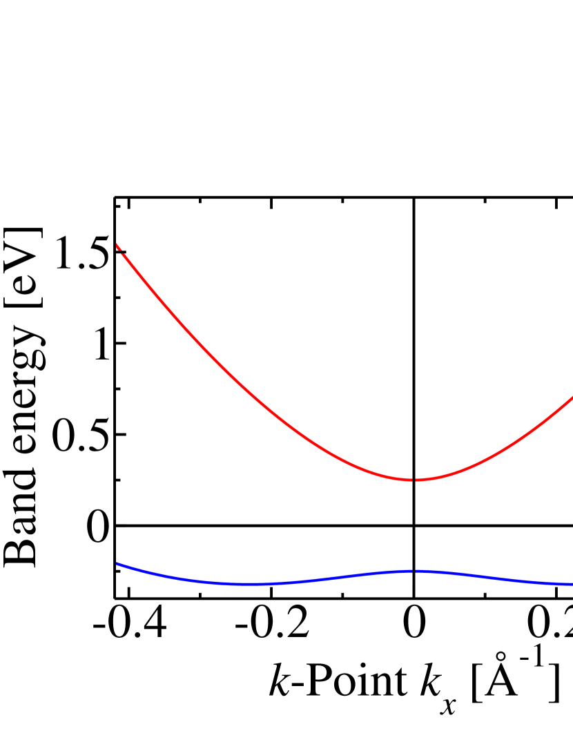
Figure 1: Band structure of the one-dimensional Rashba model.

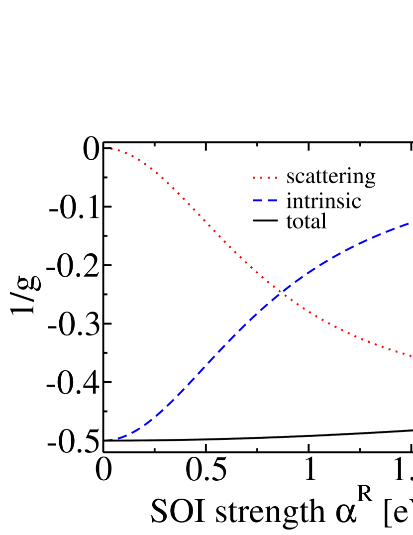
Figure 2: Inverse $g$-factor vs. SOI strength $\alpha^{\rm R}$ in the one-dimensional Rashba model.

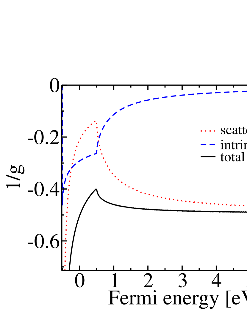
Figure 3: Inverse $g$-factor vs. Fermi energy in the one-dimensional Rashba model.

Previous theoretical works on the $g$-factor have not considered the scattering contribution Lounis et al. (2015). It is therefore important to find out whether the compensation of the decrease of the intrinsic contribution by the increase of the extrinsic contribution as discussed in Fig. 2 and Fig. 3 is peculiar to the one-dimensional Rashba model or whether it can be found in more general cases. For this reason we evaluate $g_{1}$ for the two-dimensional Rashba model. In Fig. 4 we show the inverse $g_{1}$-factor in the two-dimensional Rashba model as a function of SOI strength $\alpha^{\rm R}$ for the exchange splitting $\Delta V=1$eV and the Fermi energy $\mathcal{E}_{\rm F}=1.36$eV. Indeed for $\alpha^{\rm R}<0.5$eVÅ  the scattering corrections tend to stabilize $g_{1}$ at its non-relativistic value. However, in contrast to the one-dimensional case (Fig. 2), where $g$ does not deviate much from its nonrelativistic value up to $\alpha^{\rm R}=2$eVÅ, $g_{1}$ starts to be affected by SOI at smaller values of $\alpha^{\rm R}$ in the two-dimensional case. According to Eq. (25) the full $g$ factor is given by $g=g_{1}^{\phantom{1}}(1+M_{\rm orb}/M_{\rm spin})$. Therefore, when the scattering corrections stabilize $g_{1}$ at its nonrelativistic value the Eq. (24) is satisfied. In the two-dimensional Rashba model $M_{\rm orb}=0$ when both bands are occupied. For the Fermi energy $\mathcal{E}_{\rm F}=1.36$eV both bands are occupied and therefore $g=g_{1}$ for the range of parameters used in Fig. 4.

The inverse $g_{1}$ of the two-dimensional Rashba model is shown in Fig. 5 as a function of Fermi energy for the parameters $\Delta V=1$eV and $\alpha^{\rm R}=2$eVÅ. The scattering correction is as large as the intrinsic contribution when $\mathcal{E}_{\rm F}>1$eV. While the scattering correction is therefore important, it is not sufficiently large to bring $g_{1}$ close to its nonrelativistic value in the energy range shown in the figure, which is a major difference to the one-dimensional case illustrated in Fig. 3. According to Eq. (25) the $g$ factor is related to $g_{1}$ by $g=g_{1}M/M_{\rm spin}$. Therefore, we show in Fig. 6 the ratio $M/M_{\rm spin}$ as a function of Fermi energy. At high Fermi energy (when both bands are occupied) the orbital magnetization is zero and $M/M_{\rm spin}=1$. At low Fermi energy the sign of the orbital magnetization is opposite to the sign of the spin magnetization such that the magnitude of $M$ is smaller than the magnitude of $M_{\rm spin}$ resulting in the ratio $M/M_{\rm spin}<1$.

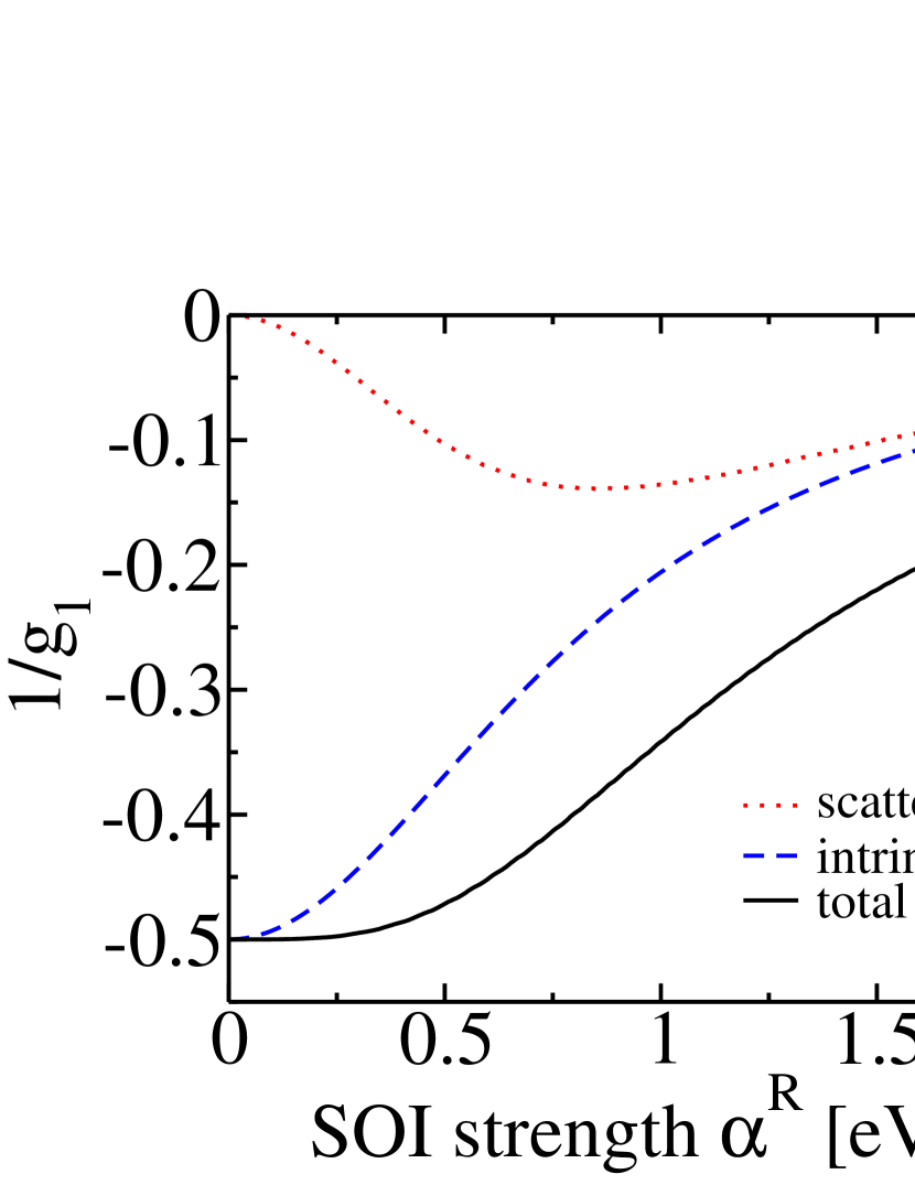
Figure 4: Inverse $g_{1}$-factor vs. SOI strength $\alpha^{\rm R}$ in the two-dimensional Rashba model.

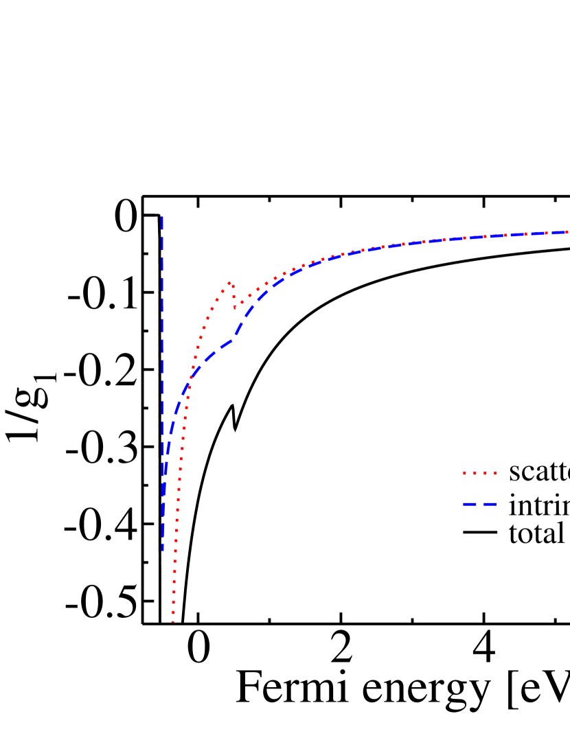
Figure 5: Inverse $g_{1}$-factor $1/g_{1}$ vs. Fermi energy in the two-dimensional Rashba model.

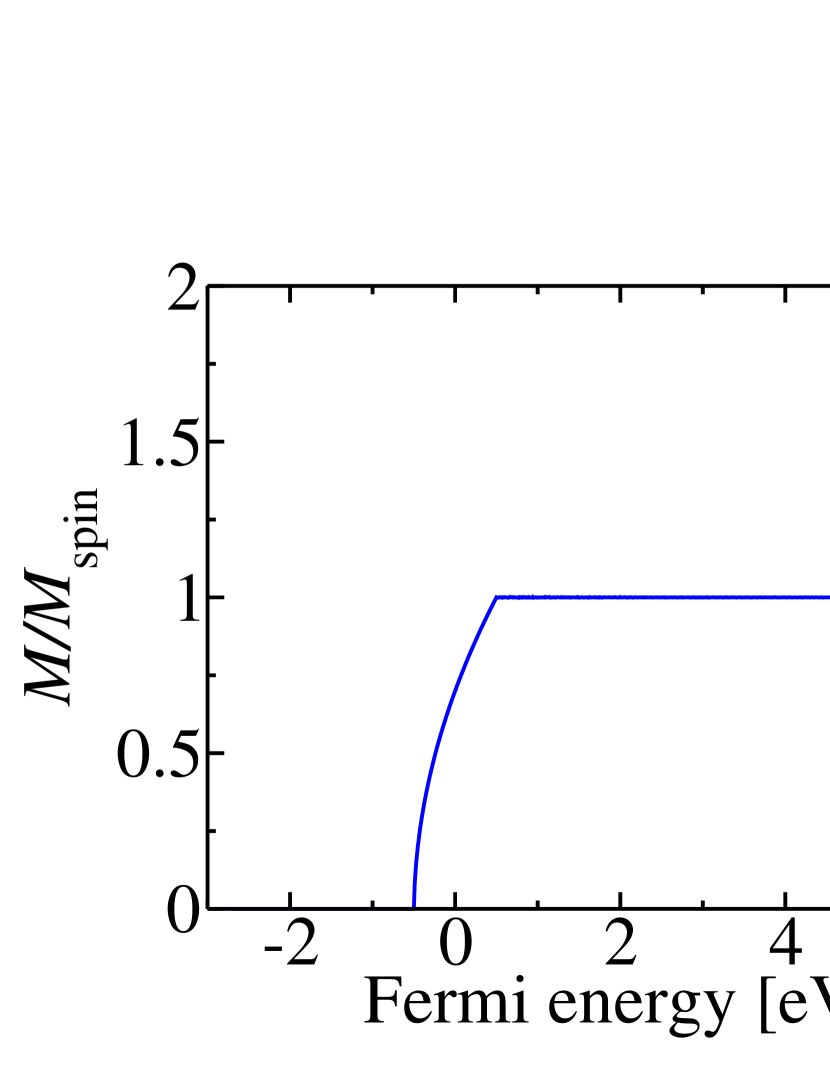
Figure 6: Ratio of total magnetization and spin magnetization, $M/M_{\rm spin}$, vs. Fermi energy in the two-dimensional Rashba model.

Next, we discuss the $g$-factor of the one-dimensional Rashba model in the noncollinear case. In Fig. 7 we plot the inverse $g$-factor and its decomposition into the intrinsic and scattering contributions as a function of the spin-spiral wave vector $q$, where exchange splitting, SOI strength and Fermi energy are set to $\Delta V=1$eV, $\alpha^{\rm R}=2$eVÅ  and $\mathcal{E}_{\rm F}=1.36$eV, respectively. Since the curves are not symmetric around $q=0$, the $g$-factor at wave number $q$ differs from the one at $-q$, i.e., the gyromagnetism in the Rashba model is chiral. At $q=-2m_{e}\alpha^{\rm R}/\hbar^{2}$ the $g$-factor assumes the value of $g=-2$ and the scattering corrections are zero. Moreover, the curves are symmetric around $q=-2m_{e}\alpha^{\rm R}/\hbar^{2}$. These observations can be explained by the concept of the effective SOI introduced in Eq. (9): At $q=-2m_{e}\alpha^{\rm R}/\hbar^{2}$ the effective SOI is zero and consequently the noncollinear magnet behaves like a collinear magnet without SOI at this value of $q$. As we have discussed above in Fig. 2, the $g$-factor of collinear magnets is $g=-2$ when SOI is absent, which explains why it is also $g=-2$ in noncollinear magnets with $q=-2m_{e}\alpha^{\rm R}/\hbar^{2}$. If only the intrinsic contribution is considered and the scattering corrections are neglected, $1/g$ varies much stronger around the point of zero effective SOI $q=-2m_{e}\alpha^{\rm R}/\hbar^{2}$, i.e., the scattering corrections stabilize $g$ at its nonrelativistic value close to the point of zero effective SOI.

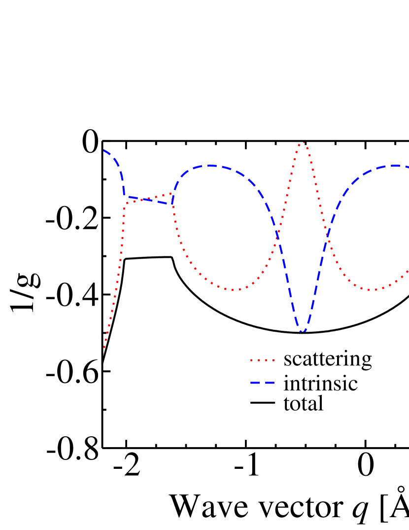
Figure 7: Inverse $g$-factor $1/g$ vs. wave number $q$ in the one-dimensional Rashba model.

III.2 Damping

We first discuss the Gilbert damping in the collinear case, i.e., we set $\hat{{\bm{M}}}({\bm{r}})=\hat{{\bm{e}}}_{z}$ in Eq. (4). The $xx$ component of the Gilbert damping is shown in Fig. 8 as a function of scattering strength $U$ for the following model parameters: exchange splitting $\Delta V=$1eV, Fermi energy $\mathcal{E}_{\rm F}=2.72$eV and SOI strength $\alpha^{\rm R}=0$. All three contributions are individually non-zero, but the contribution from the RR-vertex correction (Eq. (29)) is much smaller than the one from the AR-vertex correction (Eq. (30)) and much smaller than the intrinsic contribution (Eq. (28)). However, in this case the total damping is zero, because a non-zero damping in periodic crystals with collinear magnetization is only possible when SOI is present Garate and MacDonald (2009).

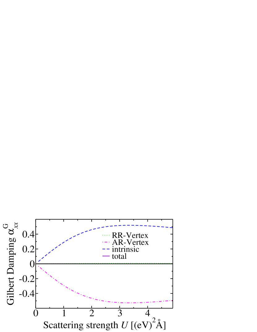
Figure 8: Gilbert damping $\alpha^{\rm G}_{xx}$ vs. scattering strength $U$ in the one-dimensional Rashba model without SOI. In this case the vertex corrections and the intrinsic contribution sum up to zero.

In Fig. 9 we show the $xx$ component of the Gilbert damping $\alpha^{\rm G}_{xx}$ as a function of scattering strength $U$ for the model parameters $\Delta V=1$eV, $\mathcal{E}_{\rm F}=2.72$eV and $\alpha^{\rm R}=2$eVÅ. The dominant contribution is the AR-vertex correction. The damping as obtained based on Eq. (10) diverges like $1/U$ in the limit $U\rightarrow 0$, i.e., proportional to the relaxation time $\tau$ Garate and MacDonald (2009). However, once the relaxation time $\tau$ is larger than the inverse frequency of the magnetization dynamics the dc-limit $\omega\rightarrow 0$ in Eq. (10) is not appropriate and $\omega>0$ needs to be used. It has been shown that the Gilbert damping is not infinite in the ballistic limit $\tau\rightarrow\infty$ when $\omega>0$ Edwards (2016); Costa and Muniz (2015). In the one-dimensional Rashba model the effective magnetic field exerted by SOI on the electron spins points in $y$ direction. Since a magnetic field along $y$ direction cannot lead to a torque in $y$ direction the $yy$ component of the Gilbert damping $\alpha^{\rm G}_{yy}$ is zero (not shown in the Figure).

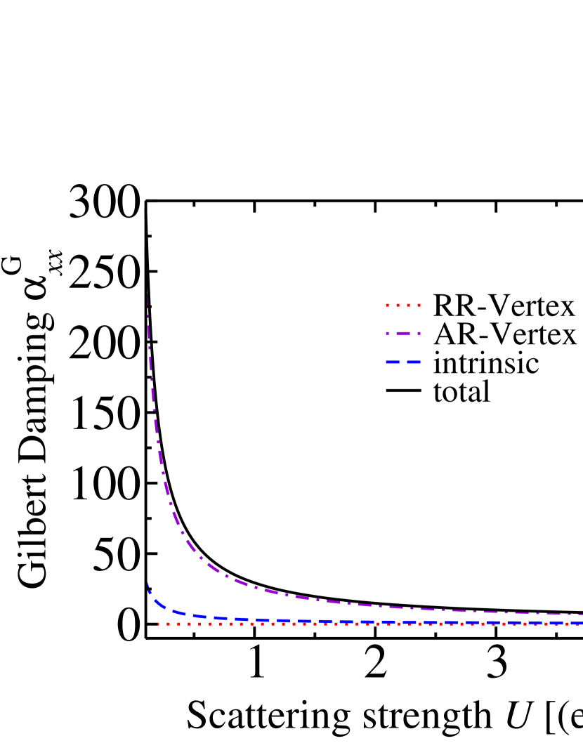
Figure 9: Gilbert damping $\alpha^{\rm G}_{xx}$ vs. scattering strength $U$ in the one-dimensional Rashba model with SOI.

Next, we discuss the Gilbert damping in the noncollinear case. In Fig. 10 we plot the $xx$ component of the Gilbert damping as a function of spin spiral wave number $q$ for the model parameters $\Delta V=1$eV, $\mathcal{E}_{\rm F}=1.36$eV, $\alpha^{\rm R}=2$eVÅ, and the scattering strength $U=0.98$(eV)²Å. The curves are symmetric around $q=-2m_{e}\alpha^{\rm R}/\hbar^{2}$, because the damping is determined by the effective SOI defined in Eq. (9). At $q=-2m_{e}\alpha^{\rm R}/\hbar^{2}$ the effective SOI is zero and therefore the total damping is zero as well. The damping at wave number $q$ differs from the one at wave number $-q$, i.e., the damping is chiral in the Rashba model. Around the point $q=-2m_{e}\alpha^{\rm R}/\hbar^{2}$ the damping is described by a quadratic parabola at first. In the regions -2Å${}^{-1}<q<$-1.2Å^-1 and 0.2Å${}^{-1}<q<$1Å^-1 this trend is interrupted by a W-shape behaviour. In the quadratic parabola region the lowest energy band crosses the Fermi energy twice. As shown in Fig. 1 the lowest band has a local maximum at $q=0$. In the W-shape region this local maximum shifts upwards, approaches the Fermi level and finally passes it such that the lowest energy band crosses the Fermi level four times. This transition in the band structure leads to oscillations in the density of states, which results in the W-shape behaviour of the Gilbert damping.

Since the damping is determined by the effective SOI, we can use Fig. 10 to draw conclusions about the damping in the noncollinear case with $\alpha^{\rm R}=0$: We only need to shift all curves in Fig. 10 to the right such that they are symmetric around $q=0$ and shift the Fermi energy. Thus, for $\alpha^{\rm R}=0$ the Gilbert damping does not vanish if $q\neq 0$. Since for $\alpha^{\rm R}=0$ angular momentum transfer from the electronic system to the lattice is not possible, the damping is purely nonlocal in this case, i.e., angular momentum is interchanged between electrons at different positions. This means that for a volume in which the magnetization of the spin-spiral in Eq. (5) performs exactly one revolution between one end of the volume and the other end the total angular momentum change associated with the damping is zero, because the angular momentum is simply redistributed within this volume and there is no net change of the angular momentum. A substantial contribution of nonlocal damping has also been predicted for domain walls in permalloy Yuan et al. (2014).

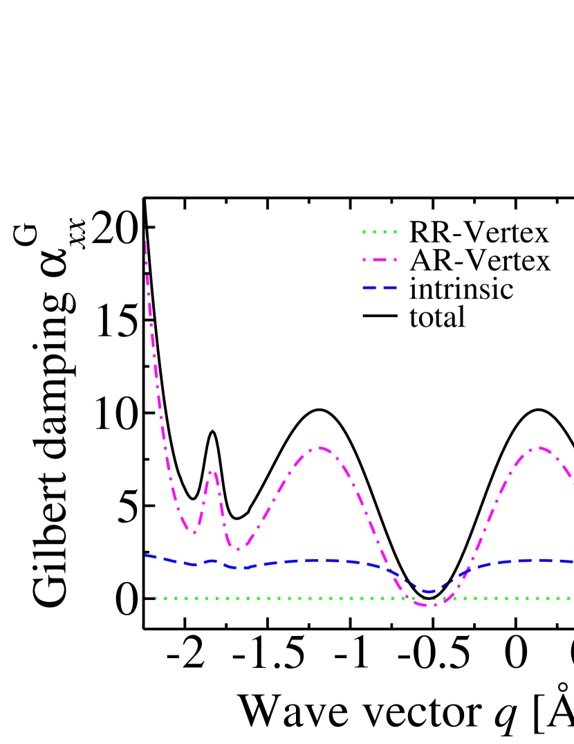
Figure 10: Gilbert damping $\alpha^{\rm G}_{xx}$ vs. spin spiral wave number $q$ in the one-dimensional Rashba model.

In Fig. 11 we plot the $yy$ component of the Gilbert damping as a function of spin spiral wave number $q$ for the model parameters $\Delta V=1$eV, $\mathcal{E}_{\rm F}=1.36$eV, $\alpha^{\rm R}=2$eVÅ, and the scattering strength $U=0.98$(eV)²Å. The total damping is zero in this case. This can be understood from the symmetry properties of the one-dimensional Rashba Hamiltonian, Eq. (4): Since this Hamiltonian is invariant when both ${\bm{\sigma}}$ and $\hat{{\bm{M}}}$ are rotated around the $y$ axis, the damping coefficient $\alpha^{\rm G}_{yy}$ does not depend on the position within the cycloidal spin spiral of Eq. (5). Therefore, nonlocal damping is not possible in this case and $\alpha^{\rm G}_{yy}$ has to be zero when $\alpha^{\rm R}=0$. It remains to be shown that $\alpha^{\rm G}_{yy}=0$ also for $\alpha^{\rm R}\neq 0$. However, this follows directly from the observation that the damping is determined by the effective SOI, Eq. (9), meaning that any case with $q\neq 0$ and $\alpha^{\rm R}\neq 0$ can always be mapped onto a case with $q\neq 0$ and $\alpha^{\rm R}=0$. As an alternative argumentation we can also invoke the finding discussed above that $\alpha^{\rm G}_{yy}=0$ in the collinear case. Since the damping is determined by the effective SOI, it follows that $\alpha^{\rm G}_{yy}=0$ also in the noncollinear case.

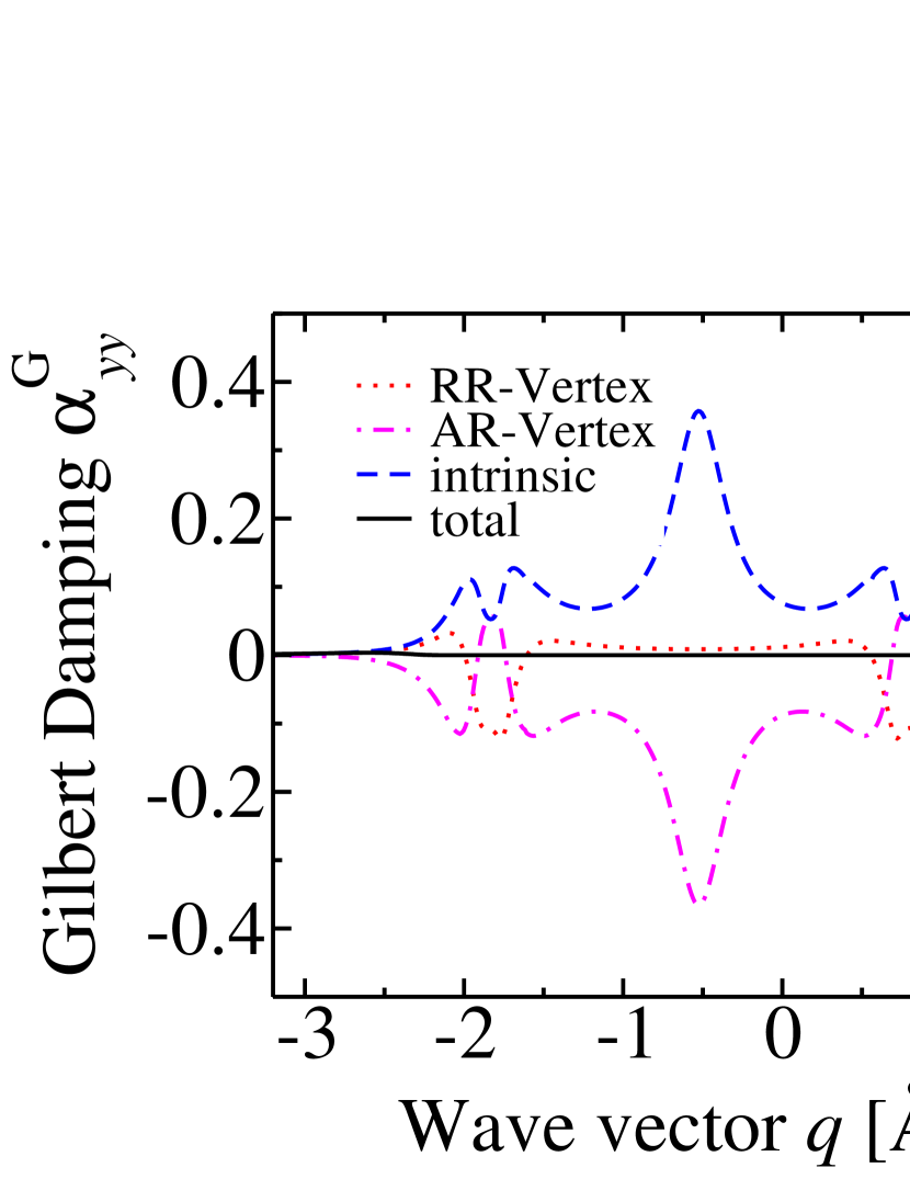
Figure 11: Gilbert damping $\alpha^{\rm G}_{yy}$ vs. spin spiral wave number $q$ in the one-dimensional Rashba model.

III.3 Current-induced torques

We first discuss the $yx$ component of the torkance. In Fig. 12 we show the torkance $t_{yx}$ as a function of the Fermi energy $\mathcal{E}_{\rm F}$ for the model parameters $\Delta V=1$eV and $\alpha^{\rm R}=2$eVÅ  when the magnetization is collinear and points in $z$ direction. We specify the torkance in units of the positive elementary charge $e$, which is a convenient choice for the one-dimensional Rashba model. When the torkance is multiplied with the electric field, we obtain the torque per length (see Eq. (34) and Ref. not ). Since the effective magnetic field from SOI points in $y$ direction, it cannot give rise to a torque in $y$ direction and consequently the total $t_{yx}$ is zero. Interestingly, the intrinsic and scattering contributions are individually nonzero. The intrinsic contribution is nonzero, because the electric field accelerates the electrons such that $\hbar\dot{k}_{x}=-eE_{x}$. Therefore, the effective magnetic field $B^{\rm SOI}_{y}=\alpha^{\rm R}k_{x}/\mu_{\rm B}$ changes as well, i.e., $\dot{B}^{\rm SOI}_{y}=\alpha^{\rm R}\dot{k}_{x}/\mu_{\rm B}=-\alpha^{\rm R}E_{x}e/(\hbar\mu_{\rm B})$. Consequently, the electron spin is no longer aligned with the total effective magnetic field (the effective magnetic field resulting from both SOI and from the exchange splitting $\Delta V$), when an electric field is applied. While the total effective magnetic field lies in the $yz$ plane, the electron spin acquires an $x$ component, because it precesses around the total effective magnetic field, with which it is not aligned due to the applied electric field Kurebayashi et al. (2014). The $x$ component of the spin density results in a torque in $y$ direction, which is the reason why the intrinsic contribution to $t_{yx}$ is nonzero. The scattering contribution to $t_{yx}$ cancels the intrinsic contribution such that the total $t_{yx}$ is zero and angular momentum conservation is satisfied.

Using the concept of effective SOI, Eq. (9), we conclude that $t_{yx}$ is also zero for the noncollinear spin-spiral described by Eq. (5). Thus, both the $y$ component of the spin-orbit torque and the nonadiabatic torque are zero for the one-dimensional Rashba model.

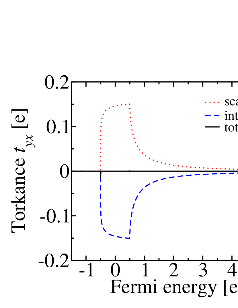
Figure 12: Torkance $t_{yx}$ vs. Fermi energy $\mathcal{E}_{\rm F}$ in the one-dimensional Rashba model.

To show that $t_{yx}=0$ is a peculiarity of the one-dimensional Rashba model, we plot in Fig. 13 the torkance $t_{yx}$ in the two-dimensional Rashba model. The intrinsic and scattering contributions depend linearly on $\alpha^{\rm R}$ for small values of $\alpha^{\rm R}$, but the slopes are opposite such that the total $t_{yx}$ is zero for sufficiently small $\alpha^{\rm R}$. However, for larger values of $\alpha^{\rm R}$ the intrinsic and scattering contributions do not cancel each other and therefore the total $t_{yx}$ becomes nonzero, in contrast to the one-dimensional Rashba model, where $t_{yx}=0$ even for large $\alpha^{\rm R}$. Several previous works determined the part of $t_{yx}$ that is proportional to $\alpha^{\rm R}$ in the two-dimensional Rashba model and found it to be zero Qaiumzadeh et al. (2015); Ado et al. (2017) for scalar disorder, which is consistent with our finding that the linear slopes of the intrinsic and scattering contributions to $t_{yx}$ are opposite for small $\alpha^{\rm R}$.

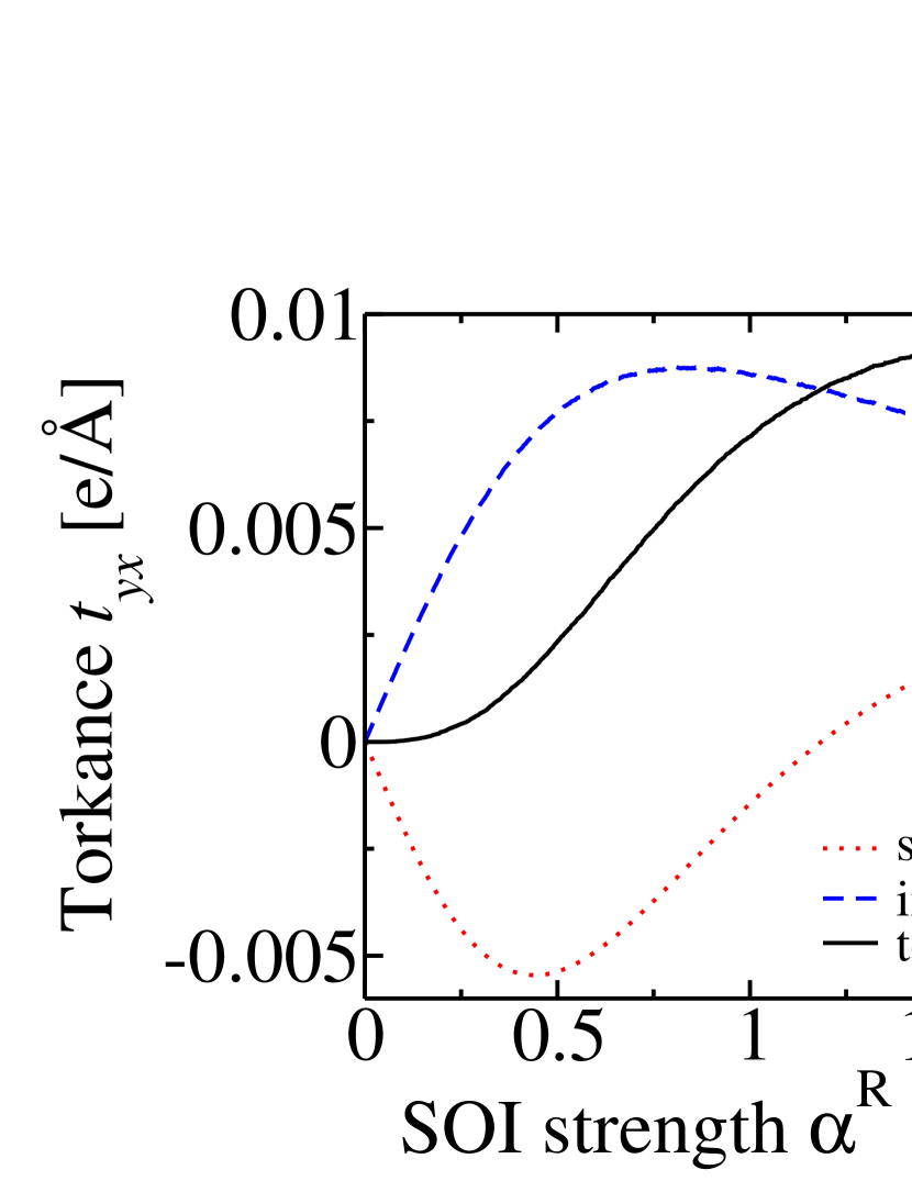
Figure 13: Nonadiabatic torkance $t_{yx}$ vs. SOI parameter $\alpha^{\rm R}$ in the two-dimensional Rashba model.

Next, we discuss the $xx$ component of the torkance in the collinear case ($\hat{{\bm{M}}}=\hat{{\bm{e}}}_{z}$). In Fig. 14 we plot the torkance $t_{xx}$ vs. scattering strength $U$ in the one-dimensional Rashba model for the parameters $\Delta V=1$eV, $\mathcal{E}_{\rm F}=2.72$eV and $\alpha^{\rm R}=2$eVÅ. The dominant contribution is the AR-type vertex correction (see Eq. (42)). $t_{xx}$ diverges like $1/U$ in the limit $U\rightarrow 0$ as expected for the odd torque in metallic systems Freimuth et al. (2014a).

In Fig. 15 and Fig. 16 we plot $t_{xx}$ as a function of spin-spiral wave number $q$ for the model parameters $\Delta V=1$eV, $\mathcal{E}_{\rm F}=2.72$eV and $U=0.18$(eV)²Å. In Fig. 15 the case with $\alpha^{\rm R}=2$eVÅ  is shown, while Fig. 16 illustrates the case with $\alpha^{\rm R}=0$. In the case $\alpha^{\rm R}=0$ the torkance $t_{xx}$ describes the spin-transfer torque (STT). In the case $\alpha^{\rm R}\neq 0$ the torkance $t_{xx}$ is the sum of contributions from STT and spin-orbit torque (SOT). The curves with $\alpha^{\rm R}=0$ and $\alpha^{\rm R}\neq 0$ are essentially related by a shift of $\Delta q=-2m_{e}\alpha^{\rm R}/\hbar^{2}$, which can be understood based on the concept of the effective SOI, Eq. (9). Thus, in the special case of the one-dimensional Rashba model STT and SOT are strongly related.

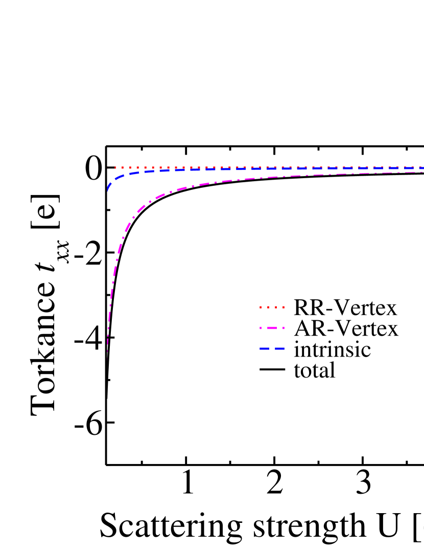
Figure 14: Torkance $t_{xx}$ vs. scattering strength $U$ in the one-dimensional Rashba model.

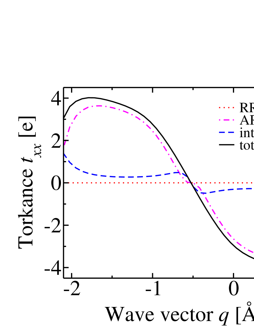
Figure 15: Torkance $t_{xx}$ vs. wave vector $q$ in the one-dimensional Rashba model with SOI.

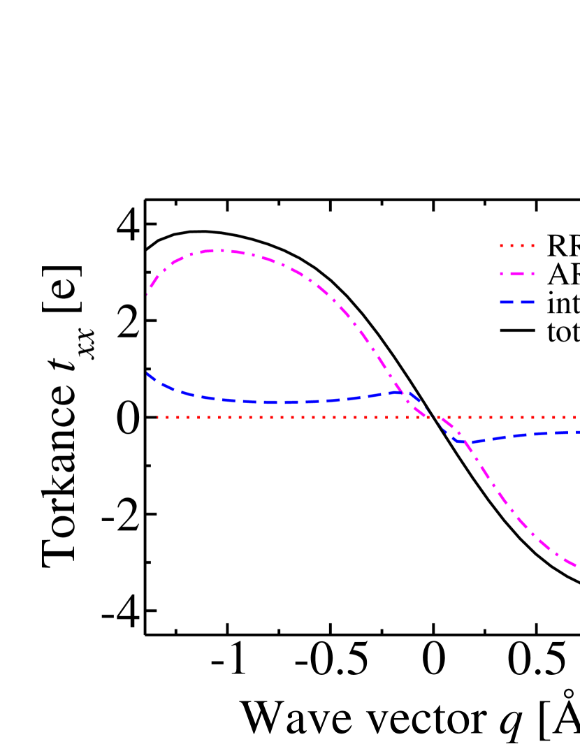
Figure 16: Torkance $t_{xx}$ vs. wave vector $q$ in the one-dimensional Rashba model without SOI.

IV Summary

We study chiral damping, chiral gyromagnetism and current-induced torques in the one-dimensional Rashba model with an additional Néel-type noncollinear magnetic exchange field. In order to describe scattering effects we use a Gaussian scalar disorder model. Scattering contributions are generally important in the one-dimensional Rashba model with the exception of the gyromagnetic ratio in the collinear case with zero SOI, where the scattering corrections vanish in the clean limit. In the one-dimensional Rashba model SOI and noncollinearity can be combined into an effective SOI. Using the concept of effective SOI, results for the magnetically collinear one-dimensional Rashba model can be used to predict the behaviour in the noncollinear case. In the noncollinear Rashba model the Gilbert damping is nonlocal and does not vanish for zero SOI. The scattering corrections tend to stabilize the gyromagnetic ratio in the one-dimensional Rashba model at its nonrelativistic value. Both the Gilbert damping and the gyromagnetic ratio are chiral for nonzero SOI strength. The antidamping-like spin-orbit torque and the nonadiabatic torque for Néel-type spin-spirals are zero in the one-dimensional Rashba model, while the antidamping-like spin-orbit torque is nonzero in the two-dimensional Rashba model for sufficiently large SOI-strength.

References

- Moriya (1960) T. Moriya, Phys. Rev. 120, 91 (1960).
- Dzyaloshinsky (1958) I. Dzyaloshinsky, Journal of Physics and Chemistry of Solids 4, 241 (1958).
- Heide et al. (2008) M. Heide, G. Bihlmayer, and S. Blügel, Phys. Rev. B 78, 140403 (2008).
- Ferriani et al. (2008) P. Ferriani, K. von Bergmann, E. Y. Vedmedenko, S. Heinze, M. Bode, M. Heide, G. Bihlmayer, S. Blügel, and R. Wiesendanger, Phys. Rev. Lett. 101, 027201 (2008).
- Yamamoto et al. (2017) K. Yamamoto, A.-M. Pradipto, K. Nawa, T. Akiyama, T. Ito, T. Ono, and K. Nakamura, AIP Advances 7, 056302 (2017).
- Lux et al. (2017) F. R. Lux, F. Freimuth, S. Blügel, and Y. Mokrousov, ArXiv e-prints (2017), eprint 1706.06068.
- Jué et al. (2015) E. Jué, C. K. Safeer, M. Drouard, A. Lopez, P. Balint, L. Buda-Prejbeanu, O. Boulle, S. Auffret, A. Schuhl, A. Manchon, et al., Nature materials 15, 272 (2015).
- Akosa et al. (2016) C. A. Akosa, I. M. Miron, G. Gaudin, and A. Manchon, Phys. Rev. B 93, 214429 (2016).
- Tserkovnyak et al. (2006) Y. Tserkovnyak, H. J. Skadsem, A. Brataas, and G. E. W. Bauer, Phys. Rev. B 74, 144405 (2006).
- Gilmore et al. (2011) K. Gilmore, I. Garate, A. H. MacDonald, and M. D. Stiles, Phys. Rev. B 84, 224412 (2011).
- Garate et al. (2009) I. Garate, K. Gilmore, M. D. Stiles, and A. H. MacDonald, Phys. Rev. B 79, 104416 (2009).
- Kim et al. (2015a) K.-W. Kim, K.-J. Lee, H.-W. Lee, and M. D. Stiles, Phys. Rev. B 92, 224426 (2015a).
- Khvalkovskiy et al. (2013) A. V. Khvalkovskiy, V. Cros, D. Apalkov, V. Nikitin, M. Krounbi, K. A. Zvezdin, A. Anane, J. Grollier, and A. Fert, Phys. Rev. B 87, 020402 (2013).
- van der Bijl and Duine (2012) E. van der Bijl and R. A. Duine, Phys. Rev. B 86, 094406 (2012).
- Freimuth et al. (2014a) F. Freimuth, S. Blügel, and Y. Mokrousov, Phys. Rev. B 90, 174423 (2014a).
- Freimuth et al. (2015) F. Freimuth, S. Blügel, and Y. Mokrousov, Phys. Rev. B 92, 064415 (2015).
- Hals and Brataas (2013) K. M. D. Hals and A. Brataas, Phys. Rev. B 88, 085423 (2013).
- Manchon and Zhang (2008) A. Manchon and S. Zhang, Phys. Rev. B 78, 212405 (2008).
- Manchon et al. (2015) A. Manchon, H. C. Koo, J. Nitta, S. M. Frolov, and R. A. Duine, Nature materials 14, 871 (2015).
- Pesin and MacDonald (2012) D. A. Pesin and A. H. MacDonald, Phys. Rev. B 86, 014416 (2012).
- Qaiumzadeh et al. (2015) A. Qaiumzadeh, R. A. Duine, and M. Titov, Phys. Rev. B 92, 014402 (2015).
- Ado et al. (2017) I. A. Ado, O. A. Tretiakov, and M. Titov, Phys. Rev. B 95, 094401 (2017).
- Kashid et al. (2014) V. Kashid, T. Schena, B. Zimmermann, Y. Mokrousov, S. Blügel, V. Shah, and H. G. Salunke, Phys. Rev. B 90, 054412 (2014).
- Schweflinghaus et al. (2016) B. Schweflinghaus, B. Zimmermann, M. Heide, G. Bihlmayer, and S. Blügel, Phys. Rev. B 94, 024403 (2016).
- Menzel et al. (2012) M. Menzel, Y. Mokrousov, R. Wieser, J. E. Bickel, E. Vedmedenko, S. Blügel, S. Heinze, K. von Bergmann, A. Kubetzka, and R. Wiesendanger, Phys. Rev. Lett. 108, 197204 (2012).
- Barke et al. (2006) I. Barke, F. Zheng, T. K. Rügheimer, and F. J. Himpsel, Phys. Rev. Lett. 97, 226405 (2006).
- Okuda et al. (2010) T. Okuda, K. Miyamaoto, Y. Takeichi, H. Miyahara, M. Ogawa, A. Harasawa, A. Kimura, I. Matsuda, A. Kakizaki, T. Shishidou, et al., Phys. Rev. B 82, 161410 (2010).
- Shick et al. (2005) A. B. Shick, F. Maca, and P. M. Oppeneer, Journal of Magnetism and Magnetic Materials 290, 257 (2005).
- Komelj et al. (2006) M. Komelj, D. Steiauf, and M. Fähnle, Phys. Rev. B 73, 134428 (2006).
- Gambardella et al. (2004) P. Gambardella, A. Dallmeyer, K. Maiti, M. C. Malagoli, S. Rusponi, P. Ohresser, W. Eberhardt, C. Carbone, and K. Kern, Phys. Rev. Lett. 93, 077203 (2004).
- Sandratskii (1986) L. M. Sandratskii, physica status solidi (b) 136, 167 (1986).
- Fujita et al. (2011) T. Fujita, M. B. A. Jalil, S. G. Tan, and S. Murakami, Journal of applied physics 110, 121301 (2011).
- Yang et al. (2015) H. Yang, A. Thiaville, S. Rohart, A. Fert, and M. Chshiev, Phys. Rev. Lett. 115, 267210 (2015).
- Yuan and Kelly (2016) Z. Yuan and P. J. Kelly, Phys. Rev. B 93, 224415 (2016).
- Yuan et al. (2014) Z. Yuan, K. M. D. Hals, Y. Liu, A. A. Starikov, A. Brataas, and P. J. Kelly, Phys. Rev. Lett. 113, 266603 (2014).
- Freimuth et al. (2013) F. Freimuth, R. Bamler, Y. Mokrousov, and A. Rosch, Phys. Rev. B 88, 214409 (2013).
- Freimuth et al. (2014b) F. Freimuth, S. Blügel, and Y. Mokrousov, Journal of physics: Condensed matter 26, 104202 (2014b).
- Freimuth et al. (2017) F. Freimuth, S. Blügel, and Y. Mokrousov, Phys. Rev. B 95, 184428 (2017).
- Kohno et al. (2016) H. Kohno, Y. Hiraoka, M. Hatami, and G. E. W. Bauer, Phys. Rev. B 94, 104417 (2016).
- Kim et al. (2015b) K.-W. Kim, K.-J. Lee, H.-W. Lee, and M. D. Stiles, Phys. Rev. B 92, 224426 (2015b).
- Edwards (2016) D. M. Edwards, Journal of Physics: Condensed Matter 28, 086004 (2016).
- Costa and Muniz (2015) A. T. Costa and R. B. Muniz, Phys. Rev. B 92, 014419 (2015).
- Brown et al. (2000) J. M. Brown, R. J. Buenker, A. Carrington, C. D. Lauro, R. N. Dixon, R. W. Field, J. T. Hougen, W. Hüttner, K. Kuchitsu, M. Mehring, et al., Molecular Physics 98, 1597 (2000).
- Kovalev et al. (2010) A. A. Kovalev, J. Sinova, and Y. Tserkovnyak, Phys. Rev. Lett. 105, 036601 (2010).
- Weischenberg et al. (2011) J. Weischenberg, F. Freimuth, J. Sinova, S. Blügel, and Y. Mokrousov, Phys. Rev. Lett. 107, 106601 (2011).
- Czaja et al. (2014) P. Czaja, F. Freimuth, J. Weischenberg, S. Blügel, and Y. Mokrousov, Phys. Rev. B 89, 014411 (2014).
- Weischenberg et al. (2013) J. Weischenberg, F. Freimuth, S. Blügel, and Y. Mokrousov, Phys. Rev. B 87, 060406 (2013).
- Qian and Vignale (2002) Z. Qian and G. Vignale, Phys. Rev. Lett. 88, 056404 (2002).
- Kittel (1949) C. Kittel, Phys. Rev. 76, 743 (1949).
- Schoen et al. (2017) M. A. W. Schoen, J. Lucassen, H. T. Nembach, T. J. Silva, B. Koopmans, C. H. Back, and J. M. Shaw, Phys. Rev. B 95, 134410 (2017).
- (51) In Ref. Freimuth et al. (2014a) and Ref. Freimuth et al. (2015) we consider the torque per unit cell and use therefore charge times length as unit of torkance. In this work we consider instead the torque per volume. Consequently, the unit of torkance used in this work is charge times length per volume. In the one-dimensional Rashba model the volume is given by the length and consequently the unit of torkance is charge.
- Lounis et al. (2015) S. Lounis, M. dos Santos Dias, and B. Schweflinghaus, Phys. Rev. B 91, 104420 (2015).
- Garate and MacDonald (2009) I. Garate and A. MacDonald, Phys. Rev. B 79, 064404 (2009).
- Kurebayashi et al. (2014) H. Kurebayashi, J. Sinova, D. Fang, A. C. Irvine, T. D. Skinner, J. Wunderlich, V. Novák, R. P. Campion, B. L. Gallagher, E. K. Vehstedt, et al., Nature nanotechnology 9, 211 (2014).