Training of Deep Neural Networks based on Distance Measures using RMSProp

Abstract

The vanishing gradient problem was a major obstacle for the success of deep learning. In recent years it was gradually alleviated through multiple different techniques. However the problem was not really overcome in a fundamental way, since it is inherent to neural networks with activation functions based on dot products. In a series of papers, we are going to analyze alternative neural network structures which are not based on dot products. In this first paper, we revisit neural networks built up of layers based on distance measures and Gaussian activation functions. These kinds of networks were only sparsely used in the past since they are hard to train when using plain stochastic gradient descent methods. We show that by using Root Mean Square Propagation (RMSProp) it is possible to efficiently learn multi-layer neural networks. Furthermore we show that when appropriately initialized these kinds of neural networks suffer much less from the vanishing and exploding gradient problem than traditional neural networks even for deep networks.

1 Introduction

Most types of neural networks nowadays are trained using stochastic gradient descent (SGD). However gradient-based approaches (batched and stochastic) suffer from several drawbacks. The most critical drawback is the vanishing gradient problem, which makes it hard to learn the parameters of the "front" layers in an $n$-layer network. This problem becomes worse as the number $n$ of layers in the architecture increases. This is especially critical in recurrent neural networks [10], which are trained by unfolding them into very deep feedforward networks. For each time step of an input sequence processed by the network a new layer is created. The second drawback of gradient-based approaches is the potential to get stuck at local minima and saddle points.

To overcome the vanishing gradient problem, several methods were proposed in the past [5][7][9][10]. Early methods consisted of the pre-training of the weights using unsupervised learning techniques in order to establish a better initial configuration, followed by a supervised fine-tuning through backpropagation. The unsupervised pre-training was used to learn generally useful feature detectors. At first, Hinton et. al. used stacked Restricted Boltzmann Machines (RBM) to do a greedy layer-wise unsupervised training of deep neural networks [9].

The Xavier Initialization [5] by Glorot et. al. (after Glorot’s first name) was a further step to overcome the vanishing gradient problem. In Xavier initialization the initial weights of the neural networks are sampled from a Gaussian distribution where the variance is a function of the number of neurons in a given layer. At about the same time Rectified Linear Units (ReLU) where introduced, a non-linearity that is scale-invariant around 0 and does not saturate at large input values [7]. Both Xavier Initialization and ReLUs alleviated the problems the sigmoid activation functions had with vanishing gradient.

Another method particularly used to cope with the vanishing gradient problem for recurrent neural networks is the Long Short-Term Memory (LSTM) network [10]. By introducing memory cells the gradient can be propagated back to a much earlier time without vanishing.

One of the newest and most effective ways to resolve the vanishing gradient problem is with residual neural networks (ResNets) [8]. ResNets yield lower training error (and test error) than their shallower counterparts simply by reintroducing outputs from shallower layers in the network to compensate for the vanishing data.

The main reason behind vanishing gradient problem is the fundamental difference between the forward and the backward pass in neural networks with activation functions based on dot products [1]. While the forward pass is highly non-linear in nature, the backward pass is completely linear due to the fixed values of the activations obtained in the forward pass. During the backpropagation the network behaves as a linear system and suffers from the problem of linear systems, which is the tendency to either explode or die when iterated.

In this paper, we address the problem of vanishing gradient by exploring the properties of neural networks based on distance measures which are an alternative to neural networks based on dot products [3]. In neural networks based on distance measures the weight vectors of neurons represent landmarks in the input space. The activation of a neuron is computed from the weighted distance of the the input vector from the corresponding landmark. Determining the distance is possible by applying different measures. In this work, we apply the most commonly used Gaussian kernel [3]. The parameters of the network to be learnt consist of both the landmarks and the weights of the distance measure.

2 Basic Principle

In this section, we show how a network of Gaussian layers interconnected in a feed-forward way can be used to approximate arbitrary bounded continuous functions. For demonstration purposes, we use a simple 1D example, see Fig. 1.

Figure 1: Network of Gaussian layers interconnected in a feed-forward way.

The input of the network is the variable $\theta\in\mathbb{R}$ restricted to the interval $\left[0,1\right]$. The first layer of the network consists of two simple 1D-Gaussian functions:

$$x^{\left(1\right)}\left(\theta\right)=\exp\left(-\frac{1}{2}\cdot\left[r_{\mathrm{x}}^{\left(0\right)}\right]^{2}\cdot\left(\theta-c_{\mathrm{x}}^{\left(0\right)}\right)^{2}\right),$$ (1)

and

$$y^{\left(1\right)}\left(\theta\right)=\exp\left(-\frac{1}{2}\cdot\left[r_{\mathrm{y}}^{\left(0\right)}\right]^{2}\cdot\left(\theta-c_{\mathrm{y}}^{\left(0\right)}\right)^{2}\right),$$ (2)

with $r_{\mathrm{x}}^{\left(0\right)},c_{\mathrm{x}}^{\left(0\right)},r_{\mathrm{y}}^{\left(1\right)},r_{\mathrm{y}}^{\left(0\right)}\in\mathbb{R}$. The shapes of (1) and (2) as functions of $\theta$ are depicted in Fig. 2.

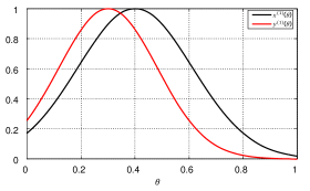
Figure 2: Activations $x^{\left(1\right)}\left(\theta\right)$ and $y^{\left(1\right)}\left(\theta\right)$ of the first hidden layer.
 Used parameters: $r_{\mathrm{x}}^{\left(0\right)}=4.7,\ c_{\mathrm{x}}^{\left(1\right)}=0.4,\ r_{\mathrm{y}}^{\left(1\right)}=5.5,\ c_{\mathrm{y}}^{\left(1\right)}=0.3$

The two outputs of the first layer can be interpreted as the x-coordinate and the y-coordinate of a 2D trajectory. The resulting trajectory is depicted in Fig. 3.

Figure 3: 2D trajectory composed of two 1D-Gaussians.

The resulting trajectory is used as input to the second layer consisting of two 2D-Gaussian functions, see Fig. 1. The upper unit is defined as follows:

$$\begin{array}[]{ccc}x^{\left(2\right)}\left(\theta\right)&=&\exp(-\frac{1}{2}\cdot\left[r_{\mathrm{x}}^{\left(1\right)}\right]^{2}\cdot\left(x^{\left(1\right)}\left(\theta\right)-c_{\mathrm{x}}^{\left(1\right)}\right)^{2}\\ &&\phantom{\exp(}-\frac{1}{2}\cdot\left[r_{\mathrm{y}}^{\left(1\right)}\right]^{2}\cdot\left(y^{\left(1\right)}\left(\theta\right)-c_{\mathrm{y}}^{\left(1\right)}\right)^{2},\end{array}$$ (3)

please note that the used 2D-Gaussian function is aligned with both axes. In particular, no rotation matrix has to be used. Next we traverse the 2D-Gaussian function along the trajectory defined by (1) and (2). The resulting trajectory in 3D space is depicted in Fig. 4.

Figure 4: Trajectory generated by traverse of a 2D-Gaussian along a path.
Used parameters: $r_{\mathrm{x}}^{\left(1\right)}=2.3,\ c_{\mathrm{x}}^{\left(1\right)}=0.5,\ r_{\mathrm{y}}^{\left(1\right)}=3.2,\ c_{\mathrm{y}}^{\left(1\right)}=0.5$

If we track a point traversing the trajectory, we see that it first climbs the 2D Gaussian function, then descends and then climbs again. Hence the resulting curve as a function of $\theta$ exhibits a higher complexity than each of the constituent parts, see Fig. 5.

Figure 5: Activation $x^{\left(2\right)}\left(\theta\right)$ of the second hidden layer as a function of $\theta$.

A curve generated in the described manner can now be used to define e.g. the x-coordinate of a much more complex path than in Fig. 3. Repeating this approach in a recursive manner allows to approximate continuous functions as demonstrated below.

To show the strength of the described method, next we are going to approximate the following function using the simple three layer network depicted in Fig. 1:

$$f\left(\theta\right)=\frac{1}{2}+\frac{1}{6}\left(\frac{\sin\left(3\pi\theta-\pi/4\right)}{\exp\left(2/5\cdot\theta\right)}+\frac{\cos\left(5\pi\theta-\pi/3\right)}{\exp\left(-4/5\cdot\theta\right)}\right)$$ (4)

The shape of (4) together with its approximation is depicted in Fig. 6. The parameters of the network are optimized using the backpropagation algorithm introduced in the next section. The (Root Mean Square) RMS of the approximation is 0.008.

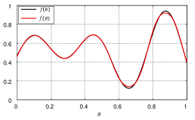
Figure 6: Approximation of a 1D-function using a 3-hidden layer network

The described method can be extended to an arbitrary number of input and output dimensions.

3 Forward Pass

Layer $l$ has $s_{l}$ inputs denoted by $a_{i}^{\left(l\right)}$ and $s_{l+1}$ outputs denoted by $a_{j}^{\left(l+1\right)}$, as depicted in Fig. 7. The value of $j$-th output depends on all $s_{l}$ inputs of layer $l$ and is calculated using the following Gaussian function:

$$a_{j}^{\left(l+1\right)}=\exp\left(-\frac{1}{2}\cdot\sum_{i=1}^{s_{l}}\left[r_{j}^{\left(l\right)}\right]_{i}^{2}\cdot\left(a_{i}^{\left(l\right)}-\left[c_{j}^{\left(l\right)}\right]_{i}\right)^{2}\right),$$ (5)

where $j\in\left\{1,\ldots,s_{l+1}\right\}$. The terms $\left[r_{j}^{\left(l\right)}\right]_{i}$ and $\left[c_{j}^{\left(l\right)}\right]_{i}$ denote the $i$-th element of vector $r_{j}^{\left(l\right)}\in\mathbb{R}^{s_{l}}$ and $c_{j}^{\left(l\right)}\in\mathbb{R}^{s_{l}}$ respectively.

Figure 7: Architecture of layer $l$ and corresponding parameters

4 Cost function

A cost function measures how well the neural network performs to map training samples $x^{\left(i\right)}$ to the desired output $y^{\left(i\right)}$. We denote the cost function with respect to a single training sample to be:

$$J\left(R,C;\ x^{\left(i\right)},y^{\left(i\right)}\right)$$ (6)

where $R$ and $C$ represent the parameters of the network based on distance measures. Given a training set of $m$ samples, the overall cost function is an average over the cost functions (6) for individual training examples plus a regularization term [6]. All cost functions typically used in practice with neural networks with activation functions based on dot products can be applied as well.

The activations of the output layer are $a_{j}^{\left(L+1\right)},\ j\in\left\{1,\ldots,s_{L+1}\right\}$, where $L$ denotes the number of layers in the network, see Fig. 8. The output activations depends both on the input $x^{\left(i\right)}$ and the parameters $R$ and $C$ of the network: $a_{j}^{\left(L+1\right)}(R,C;\ x^{\left(i\right)})$, which is implicitly assumed in following formulas.

Figure 8: Input and output activation functions of a network with $L$ layers

In particular for regression tasks we are using the quadratic cost:

$$J\left(R,C;\ x^{\left(i\right)},y^{\left(i\right)}\right)=\sum_{j=1}^{s_{L+1}}\left(a_{j}^{\left(L+1\right)}-y_{j}^{\left(i\right)}\right)^{2},$$ (7)

where $x^{\left(i\right)}\in\mathbb{R}^{s_{1}}$ is the input vector and $y^{\left(i\right)}\in\mathbb{R}^{s_{L+1}}$ is the continuous target value. For classification purposes, we use a Softmax output layer and the cross-entropy function [2]:

$$J\left(R,C;\ x^{\left(i\right)},y^{\left(i\right)}\right)=\sum_{j=1}^{s_{L+1}}y_{j}^{\left(i\right)}\log\left(\frac{\exp\ a_{j}^{\left(L+1\right)}}{\sum_{k=1}^{s_{L+1}}\exp\ a_{k}^{\left(L+1\right)}}\right),$$ (8)

where $y^{\left(i\right)}$ is a one-hot encoded target output vector. In case a Softmax output layer is used, the Gaussian activation function in last layer is omitted:

$$a_{j}^{\left(L+1\right)}=-\frac{1}{2}\cdot\sum_{i=1}^{s_{L}}\left[r_{j}^{\left(L\right)}\right]_{i}^{2}\cdot\left(a_{i}^{\left(L\right)}-\left[c_{j}^{\left(L\right)}\right]_{i}\right)^{2},$$ (9)

5 Backward pass

As in conventional neural networks backpropagation is easily adaptable [12][13]. Let us denote the partial derivative of the cost function w.r.t the activation function of layer $l+1$ as $\delta_{j}^{\left(l+1\right)}=\partial J/\partial a_{j}^{\left(l+1\right)}$.

The upper partial derivative of the predecessing layer is backpropagated using the following formula:

$$\delta_{i}^{\left(l\right)}=-\sum_{j=1}^{s_{l+1}}\delta_{j}^{\left(l+1\right)}\cdot a_{j}^{\left(l+1\right)}\cdot\left[r_{j}^{\left(l\right)}\right]_{i}^{2}\cdot\left(a_{i}^{\left(l\right)}-\left[c_{j}^{\left(l\right)}\right]_{i}\right),$$ (10)

where $i\in\left\{1,\ldots,s_{l}\right\}$. The update of the centroid parameters in layer $l$ is calculated via:

$$\frac{\partial J}{\partial\left[c_{j}^{\left(l\right)}\right]_{i}}=\delta_{j}^{\left(l+1\right)}\cdot a_{j}^{\left(l+1\right)}\cdot\left[r_{j}^{\left(l\right)}\right]_{i}^{2}\cdot\left(a_{i}^{\left(l\right)}-\left[c_{j}^{\left(l\right)}\right]_{i}\right),$$ (11)

where $j\in\left\{1,\ldots,s_{l+1}\right\}$ and $i\in\left\{1,\ldots,s_{l}\right\}$. The update of the radius parameters in layer $l$ is :

$$\frac{\partial J}{\partial\left[r_{j}^{\left(l\right)}\right]_{i}}=-\delta_{j}^{\left(l+1\right)}\cdot a_{j}^{\left(l+1\right)}\cdot\left[r_{j}^{\left(l\right)}\right]_{i}\cdot\left(a_{i}^{\left(l\right)}-\left[c_{j}^{\left(l\right)}\right]_{i}\right)^{2}.$$ (12)

6 RMSProp

It is not possible to train the neural networks based on distance measures and Gaussian activations functions using only plain mini-batch gradient descent or momentum. No or only extremely slow convergence can be achieved that way. This is the case even for shallow networks. The solution is to apply RMSProp (Root Mean Square Propagation), which renders the training possible in the first place [14].

In RMSProp, the learning rate is adapted for each of the parameter vectors $c_{j}^{\left(l\right)}$ and $r_{j}^{\left(l\right)}$, $\forall j\in\left\{1,\ldots,s_{l}\right\}$ and $\forall l\in\left\{1,\ldots,L\right\}$. The idea is to keep a moving average of the squared gradients over adjacent mini-batches for each weight:

$$\bar{v}\left(c_{j}^{\left(l\right)},\ t\right)=\gamma\bar{v}\left(c_{j}^{\left(l\right)},\ t-1\right)+\left(1-\gamma\right)\left(\partial J/\partial c_{j}^{\left(l\right)}\right)^{2}$$ (13)

$$\bar{v}\left(r_{j}^{\left(l\right)},\ t\right)=\gamma\bar{v}\left(r_{j}^{\left(l\right)},\ t-1\right)+\left(1-\gamma\right)\left(\partial J/\partial r_{j}^{\left(l\right)}\right)^{2}$$

where $\gamma$ is the forgetting factor, typically 0.9. Next the learning rate for a weight is divided by that moving average:

$$c_{j}^{\left(l\right)}:=c_{j}^{\left(l\right)}-\frac{\eta}{\sqrt{\bar{v}\left(c_{j}^{\left(l\right)},\ t\right)}}\cdot\partial J/\partial c_{j}^{\left(l\right)}$$ (14)

$$r_{j}^{\left(l\right)}:=r_{j}^{\left(l\right)}-\frac{\eta}{\sqrt{\bar{v}\left(r_{j}^{\left(l\right)},\ t\right)}}\cdot\partial J/\partial r_{j}^{\left(l\right)}$$

RMSProp has shown excellent adaptation of learning rate in different applications.

7 Initialization

As in neural networks based on dot products [5], a sensible initialization of the weights is crucial for convergence, especially when training deep neural networks. The initialization of the weights controlling the center of the Gaussian functions is straightforward:

$$\left[c_{j}^{\left(l\right)}\right]_{i}\in\mathcal{N}\left(\mu_{\mathrm{c}},\ \sigma_{\mathrm{c}}^{2}\right),$$ (15)

where $\mathcal{N}$ denotes a normal distribution. Experiments show that values $\mu_{\mathrm{c}}=0.63$ and $\sigma_{\mathrm{c}}=0.1$ work well for most network architectures. The initialization in (15) does not depend neither on the number of inputs nor on the number of outputs of a layer.

The initialization of the weights controlling the radii of the Gaussian functions is slightly more complicated:

$$\left[r_{j}^{\left(l\right)}\right]_{i}\in\mathcal{N}\left(\mu_{\mathrm{r}},\ \sigma_{\mathrm{r}}^{2}\right),$$ (16)

with

$$\mu_{\mathrm{r}}=\sqrt{\frac{2\cdot\ln\left(1/\epsilon\right)}{s_{l}}},\ \sigma_{\mathrm{r}}=f_{\mathrm{r}}\cdot\mu_{\mathrm{r}},$$ (17)

where typically $\epsilon=0.1$ and $f_{\mathrm{r}}=0.4$. For breaking the symmetry setting $f_{\mathrm{r}}>0$ is important. The detailed derivation of (17) will be presented in a separate paper.

Using the above method, we next initialize a network consisting of $L=170$ layers with $s_{1}=784$ nodes in the input layer and $s_{l}=50$ nodes in each consecutive layer. The input signal is uniformly distributed between 0 and 1. The histograms of the first node in layer $l=50$, $l=100$ and $l=150$ is depicted in Fig. 9.

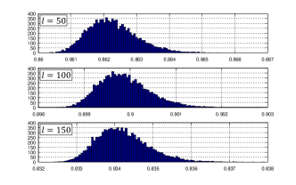
Figure 9: Histograms of the first node in layer $l=50$, $l=100$ and $l=150$.

Although the variance of the activations is slightly decreasing with every layer, it is not vanishing until only very late layers [5]. Furthermore no dying or saturated neurons are observed as is the case of ReLUs [11]. Same behaviour is observed for the backpropagted gradients $\delta_{i}^{\left(l\right)}$ in (10).

8 Alternating Optimization Method

We discovered a technique, which improves the convergence in training deep neural networks ($L>50$) drastically. The trick is to optimize the sets of weights $r_{j}^{\left(l\right)}$ and $c_{j}^{\left(l\right)}$ for all nodes and all layers in an alternating way. For a certain number of iterations $i_{c}$ during an epoch only weights $r_{j}^{\left(l\right)}$ are optimized, while $c_{j}^{\left(l\right)}$ are treated as constants. Then for a certain number of iterations $i_{r}$ the opposite is done. Subsequently, the first step is repeated again and so on. As a finalization step in late epochs optionally a combined optimization can be performed. A positive side effect of applying the alternating optimization method lies in the reduced computational load.

9 Regularization

To help prevent overfitting, we make use of L2 regularization (also called a weight decay term). Since two sets of parameters are optimized in neural networks based on distance measures the overall cost function is of the form:

$$J\left(R,C\right) =\frac{1}{m}\sum_{i=1}^{m}J\left(R,C;\ x^{\left(i\right)},y^{\left(i\right)}\right)$$ (18)

$$+\frac{\lambda_{\mathrm{c}}}{2}\sum_{l=1}^{L}\sum_{i=1}^{s_{l}}\sum_{j=1}^{s_{l+1}}\left[c_{j}^{\left(l\right)}\right]_{i}^{2}+\frac{\lambda_{\mathrm{r}}}{2}\sum_{l=1}^{L}\sum_{i=1}^{s_{l}}\sum_{j=1}^{s_{l+1}}\left[r_{j}^{\left(l\right)}\right]_{i}^{2}$$

where $m$ denotes the number of samples in the training set and $\lambda_{\mathrm{c}}$ and $\lambda_{\mathrm{r}}$ are the regularization strengths. In general $\lambda_{\mathrm{c}}$ and $\lambda_{\mathrm{r}}$ have to be selected independently for getting optimal results. The second and third term in (18) tend to decrease the magnitude of the weights, and thus helps prevent overfitting.

Another way of preventing overfitting when using neural networks based on distance measures is to apply the alternating optimization method introduced in the previous section. Optimizing only for the half of the coefficients at each moment reduces the actual number of degrees of freedom, though acting as a form of regularization.

10 Experiments

10.1 MNIST

In this subsection we demonstrate that the classification performance of the presented neural networks based on distance measures and Gaussian activation functions is comparable to the classification performance of traditional neural networks. To this end we use the well-known MNIST benchmark of handwritten digit images. MNIST consists of two datasets of handwritten digits of size 28x28 pixels, one for training (60,000 images) and one for testing (10,000 images). The goal of the experiment is not primarily to achieve state-of-the-art results, which would require convolutional layers and novel elastic training image deformations.

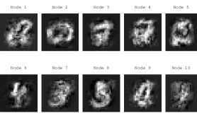
Figure 10: Learned first layer weights $c_{j}^{\left(1\right)},\ j\in\left\{1,\ldots 10\right\}$ at the end of learning for MNIST

The input signal consists of raw pixel intensities of the original gray scale images mapped to real values pixel intensity range from 0 (background) to 1 (max foreground intensity). The dimension of the input signal is 28x28 = 784. The network architecture is built up of 2 fully-connected hidden layers with 100 units in each layer. We use the cross-entropy cost function in (7) and apply regularization (18) only to the radii terms, i.e. $\lambda_{\mathrm{c}}=0$. We use a variable learning rate that shrinks by a multiplicative constant after each epoch.

The test set accuracy after 30 epochs is 98.2%, which is a comparable result to a traditional neural networks with approx. the same number of parameters [4]. The weights of the first layer are depicted in Fig. 10 and Fig. 11.

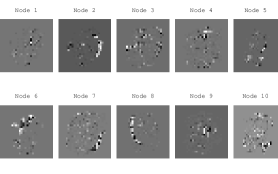
Figure 11: Learned first layer weights $r_{j}^{\left(1\right)},\ j\in\left\{1,\ldots 10\right\}$ at the end of learning for MNIST

10.2 Images

In this section we demonstrate the ability of the presented neural networks based on distance measures and Gaussian activation functions to approximate arbitrary functions. To this end we use a small 32x32 grayscale natural image. Images in its most general form can be interpreted as functions $f$ from $\mathbb{R}^{2}$ to $\mathbb{R}$. We use a small fully-connected network with 2 hidden layers and 10 nodes in each layer. The input of the network consists of pixel coordinates $\left(x,\ y\right)$. The desired output is merely the grayvalue at the corresponding pixel coordinate. We apply a full batch gradient descent. We use the quadratic cost in (7) and no regularization to utilize all degrees of freedom. The result of the approximation is depicted in Fig. 12.

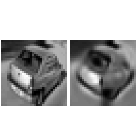
Figure 12: 32x32 natural grayscale image (left) and its approximation using a network with 2 hidden layers

Since neural networks in general are capable of approximating only continuous functions, the approximated image exhibits a blurry appearance. With a slightly increased number of layers and hidden units the approximation can be made indistinguishable from the original.

10.3 Approximating a probability density function

In the last example, we approximate a simple probability density function (pdf) consisting of a bivariate Gaussian distribution with a covariance matrix not being the identity matrix , i.e. a rotated Gaussian function, see. Fig. 13:

$$p_{\mathbf{X}}\left(\mathbf{x}\right)=\frac{1}{2\pi\sqrt{\left|\Sigma\right|}}\exp\left(-\frac{1}{2}(\mathbf{x}-\mathbf{\mu})^{\mathrm{T}}\mathbf{\Sigma}^{-1}(\mathbf{x}-\mathbf{\mu})^{\mathrm{T}}\right)$$ (19)

where

$$\mathbf{\mu}=\left(\begin{array}[]{c}-0.5\\ 0.5\end{array}\right),\ \mathbf{\Sigma}=\left(\begin{array}[]{cc}0.30&0.36\\ 0.36&1.20\end{array}\right).$$ (20)

Since each layer in neural networks based on distance measures and Gaussian activation functions consists only of Gaussian functions aligned with the main axes (5), we want to see how well a minimal network consisting of 1 fully-connected hidden layer with 2 units is able to approximate this function. The result is depicted on the right hand side of Fig. 13. The approximation in the the vicinity of the peak is excellent. In the surrounding area a slight distortion is visible. The overall RMS of the approximation is 0.006.

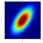
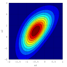
Figure 13: Bivariate Gaussian distribution with a non-diagonal covariance matrix and its approximation

11 Conclusions and Future Work

In this paper, we have revisited neural network structures based on distance measures and Gaussian activation functions. We showed that training of these type of neural network is only feasible when using the stochastic gradient descent in combination with RMSProp. We showed also that with a proper initialization of the networks the vanishing gradient problem is much less than in traditional neural networks.

In our future work we will examine neural network architectures which are built up of combinations of traditional layers and layers based on distance measures and Gaussian activation functions introduced in this paper. In particular the use of layers based on distance measures in the output layer is showing very promising results. Currently we are analyzing the performance of neural networks based on distance measures when used in deep recurrent networks.

References

- [1] Christopher M. Bishop and Geoffrey Hinton. Neural Networks For Pattern Recognition. Oxford University Press, 2005.
- [2] Pieter-Tjerk de Boer, Dirk Kroese, Shie Mannor, and Reuven Y. Rubinstein. A tutorial on the cross-entropy method. Annals of Operations Research, pages 19–67, 2005.
- [3] Klaus Debes, Alexander Koenig, and Horst-Michael Gross. Transfer functions in artificial neural networks. Journal of New Media in Neural and Cognitive Science and Education, 2005.
- [4] D. Erhan, P. Manzagol, Y. Bengio, S. Bengio, and P. Vincent. The difficulty of training deep architectures and the effect of unsupervised pre-training. AISTATS, 5:153–160, 2009.
- [5] X. Glorot and Y. Bengio. Understanding the difficulty of training deep feedforward neural networks. International conference on artificial intelligence and statistics, pages 249–256, 2010.
- [6] Ian Goodfellow, Yoshua Bengio, and Aaron Courville. Deep Learning. MIT Press, 2016. http://www.deeplearningbook.org.
- [7] R Hahnloser, R. Sarpeshkar, M A Mahowald, R. J. Douglas, and H.S. Seung. Digital selection and analogue amplification coexist in a cortex-inspired silicon circuit. Nature, 405:947–951, 2000.
- [8] K. He, X. Zhang, S. Ren, and J. Sun. Deep Residual Learning for Image Recognition. ArXiv e-prints, December 2015.
- [9] Geoffrey E. Hinton, Simon Osindero, and Yee-Whye Teh. A fast learning algorithm for deep belief nets. Neural Computation, 7:1527–1554, 2006.
- [10] Sepp Hochreiter and Juergen Schmidhuber. Long short-term memory. Neural Computation. 9, pages 1735–1780, 1997.
- [11] Andrew L. Maas, Awni Y. Hannun, and Andrew Y. Ng. Rectifier nonlinearities improve neural network acoustic models. Proc. ICML, 1, 2013.
- [12] David E. Rumelhart, Geoffrey E. Hinton, and Ronald J. Williams. Learning representations by back-propagating errors. Nature, 323:33–536, 1986.
- [13] Juergen Schmidhuber. Deep learning in neural networks: An overview. Neural Networks, 61:85–117, 2015.
- [14] T. Tieleman and G. Hinton. Lecture 6.5—rmsprop: Divide the gradient by a running average of its recent magnitude. COURSERA: Neural Networks for Machine Learning, 2012.