$q$-deformed Einstein’s Model to Describe Specific Heat of Solid

Abstract

Realistic phenomena can be described more appropriately using generalized canonical ensemble, with proper parameter sets involved. We have generalized the Einstein’s theory for specific heat of solid in Tsallis statistics, where the temperature fluctuation is introduced into the theory via the fluctuation parameter $q$. At low temperature the Einstein’s curve of the specific heat in the nonextensive Tsallis scenario exactly lies on the experimental data points. Consequently this $q$-modified Einstein’s curve is found to be overlapping with the one predicted by Debye. Considering only the temperature fluctuation effect(even without considering more than one mode of vibration is being triggered) we found that the $C_{V}$ vs $T$ curve is as good as obtained by considering the different modes of vibration as suggested by Debye. Generalizing the Einstein’s theory in Tsallis statistics we found that a unique value of the Einstein temperature $\theta_{E}$ along with a temperature dependent deformation parameter $q(T)$, can well describe the phenomena of specific heat of solid i.e. the theory is equivalent to Debye’s theory with a temperature dependent $\theta_{D}$.

Keywords: Tsallis statistics, temperature fluctuation, specific heat of solid, Einstein’s theory, Debye’s modification.

1 Introduction

Statistical mechanics has been proved to be one of the most powerful tools in various domains over the last century. It has been successfully used not only in different branch of physics (e.g. condensed matter physics, high energy physics, Astrophysics etc.), but in different areas beyond those (e.g. share price dynamics, dynamics related to traffic control etc). The results predicted by the Statistical Mechanics have been found to be in good agreement with the experiments. The important fact here is that one can predict the macroscopic properties of the system without having much detailed knowledge of each and every microstate of the system, but based on the notion of the statistical average of the microscopic properties.

Attempts have been made to generalize this important tool (i.e. statistical mechanics) in recent years[1, 2, 3]. This generalized statistical techniques(popularly known as superstatistics or nonextensive statistics (in Tsallis statistics $q$ being the deformation parameter)) have been applied to a wide range of complex systems, e.g., hydrodynamic turbulence, defect turbulence, share price dynamics, random matrix theory, random networks, wind velocity fluctuations, hydroclimatic fluctuations, the statistics of train departure delays and models of the metastatic cascade in cancerous systems [4, 5, 6, 7, 9, 8, 10].

In this approach, the key parameter is the inverse temperature parameter $\beta~{}(=1/k_{B}T)$ which exhibits fluctuations(e.g. in turbulent system with energy dissipation) on a large time scale. These type of complex systems can be modelled by superposition of ordinary statistical mechanics with varying temperature parameters, which is called superstatistics or deformed statistics to sum up. The stationary distributions of deformed/superstatistical systems differs from the usual Boltzmann-type statistical mechanics and they can disclose themselves into asymptotic power laws or some different functional forms in the energy $E$ [11, 12, 13].

By using the non-extensive statistical methods one can incorporate the fact of temperature fluctuations and the proceeding sections are devoted mainly for an attempt to give more insight on it [3, 14, 15, 16]. This approach deals with the fluctuation parameter $q$ which corresponds to the degree of the temperature fluctuation effect to the concerned system. Detailed theoretical studies for nonextensive systems can be found in [17, 18, 19]. In this formalism we can treat our normal Boltzmann-Gibbs statistics as a special case of this generalized one, where temperature fluctuation effects are negligible, corresponds to $q=1.0$. More deviation of $q$ from the value $1.0$ denotes a system with more fluctuating temperature. Various works related to this generalized or nonextensive statistics have been reported in different phenomena [3, 20, 21, 22, 23]. More works have been done on theoretical understanding as well as different applications [24, 25, 26, 27, 28, 29, 30, 31, 32, 33, 34, 35, 36, 37, 38, 39, 40, 41, 42, 43, 44].

2 Temperature fluctuation and the modified entropy

The phenomena of temperature fluctuation can be interpreted physically as the deformation of a ideal canonical ensemble to a more realistic case. Ideal canonical ensemble is supposed to be the statistical ensemble that represents the possible states of a mechanical system in thermal equilibrium with a heat bath at a fixed temperature, say $T$. Consequently each and every cell(very small identical portions of the system) will be at temperature $T$. To make it more realistic we can think about a modified canonical system which is in thermal equilibrium with a heat bath at a fixed temperature $T$ but there will be a small variation in temperature in different cells, say between $T-\delta T$ to $T+\delta T$, though the average temperature of the system will be $T$ still.

A connection between the entropy ($s$) and the number of microstates ($\Omega$) of a system can be derived intuitively as follows. We know the entropy is a measure of the degree of randomness of a system i.e. the number of possible microscopic configuration. The only thing we can infer clearly is that, they both $s$ and $\Omega$ will increase (or decrease) together. Assuming $s=f(\Omega)$ and noting that the entropy is additive and the number of microstates is multiplicative, a simple calculation yields $s=k_{B}\ln\Omega$.

A more general connection between $s$ and $\Omega$ can be made (in the context of generalized/deformed statistics) which will deform the fundamental relation as

$$s=f(\Omega^{q}),$$ (1)

where the deformation parameter $q>0$. Subsequently, the generalized entropy can be shown to take the following form.

$$s_{q}=k_{B}\ln_{q}\Omega$$ (2)

where the generalized log function($\ln_{q}\Omega$) is defined as

$$\ln_{q}\Omega=\frac{\Omega^{1-q}-1}{1-q}.$$ (3)

Consequently the generalized exponential function becomes

$$e_{q}^{x}=\left[1+(1-q)x\right]^{\frac{1}{1-q}}.$$ (4)

Therefore $q$-modified Shannon entropy takes the following form

$$s_{q}=k_{B}\frac{\sum p_{i}^{q}-1}{1-q}$$ (5)

Extremizing $s_{q}$ subject to suitable constraints yields more general canonical ensembles(see B), where the probability to observe a microstate with energy $\epsilon_{i}$ is given by: [1, 45, 46]

$$p_{i}=\frac{e_{q}^{-\beta^{\prime}\epsilon_{i}}}{Z_{q}}=\frac{1}{Z_{q}}\left[1-(1-q)\beta^{\prime}\epsilon_{i}\right]^{\frac{1}{1-q}}$$ (6)

with partition function $Z_{q}$ and inverse temperature parameter $\beta=\frac{1}{k_{B}T}$. Also $\beta^{\prime}$ is the $q$-modified quantity and is given by [1, 45]

$$\beta^{\prime}=\frac{\beta}{\sum_{i}p_{i}^{q}+(1-q)\beta u_{q}}=\frac{\beta}{Z_{q}^{1-q}+(1-q)\beta u_{q}}$$ (7)

with $q$-generalized average energy

$$u_{q}=\frac{\sum_{i}\epsilon_{i}p_{i}^{q}}{\sum_{i}p_{i}^{q}}$$ (8)

The $q$-deformed/generalized exponential function can be expanded as follows

$$e_{q}^{x} = \left[1+(1-q)x\right]^{\frac{1}{1-q}}$$ (9)

$$= 1+x+q\frac{x^{2}}{2!}+q(2q-1)\frac{x^{3}}{3!}+q(2q-1)(3q-2)\frac{x^{4}}{4!}+\cdots$$

where $x=-\beta\epsilon_{i}=-\frac{\epsilon_{i}}{k_{B}T}$. The $q$ factors in the expansion, which can be absorbed in $T$, will account for the temperature fluctuation of the system. By setting $q=1.0$ (which corresponds to zero or negligible temperature fluctuation) one gets back the normal Boltzmann-Gibbs statistics.

3 Specific heat of solid in the light of Tsallis statistics

From the previous discussion it is evident that we can use this generalized/deformed statistical mechanics wherever the system is subjected to some kind of temperature fluctuation. If the temperature fluctuation effect is not negligible enough to disclose itself, then definitely there will be some deviation from the ideal phenomena.

3.1 Einstein’s theory of specific heat

Einstein viewed the specific heat of solid as an effect of the vibrations of the solid. He treated the atoms in a $N$-atoms solid (e.g. crystal) as $N$ 3-D simple harmonic oscillators, each of which is vibrating with the common frequency $\nu_{E}$. The magnitude of $\nu_{E}$ depends on the strength of the restoring force acting on each atom(which in this case considered to be the same for each atom). Now we know a solid of $N$ atoms is equivalent to $3\rm{N}$ 1-D harmonic oscillators. So we can treat each atom as a collection of 3 vibrating 1-D harmonic oscillators and all the $3\rm{N}$ 1-D oscillators are vibrating with a common frequency $\nu_{E}$. This kind of treatment is a gross approximation as the lattice vibrations, in reality, are very complicated coupled oscillations [47, 48, 49, 50].

The energy levels of the one-dimensional harmonic oscillator can be written as

$$\epsilon_{n}=\left(n+\frac{1}{2}\right)h\nu_{E}$$ (10)

where $h$ is the Planck constant and $n=0,1,2,\cdots$. In the treatment of canonical ensemble all such 1-D oscillators are in thermal equilibrium (say, at temperature $T$). For a single 1-D oscillator, the partition function($Z$) can be written as

$$Z = \sum_{n=0}^{\infty}\exp\left(-\beta\epsilon_{n}\right)$$ (11)

$$= \sum_{n=0}^{\infty}\exp\left\{-\beta\left(n+\frac{1}{2}\right)h\nu_{E}\right\}$$

$$= e^{-x/2}\sum_{n=0}^{\infty}e^{-nx}=\frac{e^{-x/2}}{1-e^{-x}},~{}~{}\rm{where}~{}x=\beta h\nu_{E}$$

In above, we have used the fact that $\sum_{n=0}^{\infty}x^{n}=\frac{1}{1-x}$. Accordingly, the mean energy of a single oscillator is found to be

$$u = \sum_{n=0}^{\infty}\frac{\epsilon_{n}\exp\left(-\beta\epsilon_{n}\right)}{Z}$$ (12)

$$= -\frac{\partial\left(\ln Z\right)}{\partial\beta}=\frac{\partial}{\partial\beta}\left\{\frac{\beta h\nu_{E}}{2}+\ln\left(1-e^{-\beta h\nu_{E}}\right)\right\}=\frac{h\nu_{E}}{2}+\frac{h\nu_{E}}{e^{\beta h\nu_{E}}-1}$$

Here $\frac{h\nu_{E}}{2}$ is the zero point energy. The energy of the $3N$ 1-D oscillators in the $N$-atom solid is given by

$$U=3Nu=3N\left(\frac{h\nu_{E}}{2}+\frac{h\nu_{E}}{e^{\beta h\nu_{E}}-1}\right)$$ (13)

We write the heat capacity at constant volume as

$$C_{V} = \left(\frac{\partial U}{\partial T}\right)_{V}$$ (14)

$$= 3N\left(\frac{\partial U}{\partial\beta}\right)_{V}\left(\frac{\partial\beta}{\partial T}\right)=3Nk_{B}\frac{x^{2}e^{x}}{\left(e^{x}-1\right)^{2}},~{}~{}\rm{with}~{}x=\frac{h\nu_{E}}{k_{B}T}=\frac{\theta_{E}}{T}.$$

In above $\theta_{E}$ is called the ”Einstein temperature”. It is different for different solid and reflects the lattice rigidity. Now when the temperature is very high i.e. $T\gg\theta_{E}$ (i.e. $x\ll 1$), the Einstein heat capacity reduces to $C_{V}=3Nk_{B}$ which is the Dulong and Petit law. We set $e^{x}\sim 1+x$ in the denominator of the specific heat expression above (Eq. 14)for small $x$ while getting the Dulong and Petit law.

When the temperature is low i.e. when $T\ll\theta_{E}$ (i.e., $x\gg 1$), the Einstein specific heat $C_{V}\rightarrow 0$ as $T\rightarrow 0$. This is obtained by setting $e^{x}-1\sim e^{x}$ in the denominator of the specific heat expression (Eq. 14) for large $x$. This is also a requirement which follows from the third law of thermodynamics.

3.2 Debye’s modification to Einstein’s model of specific heat

Debye did a major improvement of the Einstein’s model. He treated the coupled vibrations of the solid in terms of $3N$ normal modes of vibration of the entire solid, each with its own frequency. So in his treatment the lattice vibrations are equivalent to $3N$ independent harmonic oscillators with different normal mode frequencies. The crystal for low frequency vibrations can be treated as a homogeneous elastic medium. For the low frequencies, the wavelength $\lambda\gg a$, where $a$ is the atomic spacing. The normal modes mentioned above, are defined as the frequencies of the standing waves. The number of normal modes with the frequency ranges between $\nu$ and $\nu+d\nu$ in such a medium [51, 48, 49, 50].

$$g(\nu)d\nu=\frac{4\pi V\nu^{2}}{v^{3}}d\nu$$ (15)

where $V$ is the volume of the crystal and $v$ is the propagation velocity of the wave in solid. The expression mentioned above(Eq.(15)), is applicable only to the low frequency vibrations in a crystal. The approximation used by Debye to make the form useful is that the expression(Eq.(15)) applies to all frequencies, and he established the concept of a maximum frequency $\nu_{D}$ (the Debye frequency) to ensure the total number of modes to be $3N$, i.e., $\int_{0}^{\nu_{D}}g(\nu)d\nu=3N$. Now we can integrate over all of the frequencies to find the internal energy of the crystal with the approximation discussed above, as suggested by Debye. Hence in Debye’s theory the heat capacity is given by

$$C_{V}=\left(\frac{\partial U}{\partial T}\right)_{V}=3Nk_{B}\left\{\frac{3}{x_{D}^{3}}\int_{0}^{x_{D}}\frac{x^{4}e^{x}}{\left(e^{x}-1\right)^{2}}dx\right\}$$ (16)

where $x=\frac{h\nu}{k_{B}T}$, and $x_{D}=\frac{h\nu_{D}}{k_{B}T}=\frac{\theta_{D}}{T}$, where $\theta_{D}$ is the Debye temperature. Clearly $C_{V}$ depends on $\theta_{D}$. Analytically we cannot evaluate the integral, it has to be done numerically. At high temperatures ($T\gg\theta_{D},~{}x_{D}\ll 1$), we can give a compact form to the integrand, rewriting in the following way:

$$\frac{x^{4}e^{x}}{\left(e^{x}-1\right)^{2}}=\frac{x^{4}}{\left(e^{x}-1\right)\left(1-e^{-x}\right)}=\frac{x^{4}}{2\left(\cosh(x)-1\right)}=\frac{x^{4}}{2\left(\frac{x^{2}}{2!}+\frac{x^{4}}{4!}+\cdots\right)}$$ (17)

Keeping only the $x^{2}$ term in the denominator we get

$$C_{V}=3Nk_{B}\left\{\frac{3}{x_{D}^{3}}\int_{0}^{x_{D}}x^{2}dx\right\}=3Nk_{B}$$ (18)

which is the Dulong and Petit law. To determine the heat capacity at the low temperature limit ($T\ll\theta_{D},~{}x_{D}\gg 1$), we see that the integrand (in Eq.(16)) tends towards zero rapidly for large $x$. We replace the upper limit by $\infty$ and turn the integral into a standard integral to give

$$C_{V}=3Nk_{B}\left(\frac{T}{\theta_{D}}\right)^{3}\left\{3\int_{0}^{\infty}\frac{x^{4}e^{x}}{\left(e^{x}-1\right)^{2}}\right\}=\frac{12}{5}\pi^{4}Nk_{B}\left(\frac{T}{\theta_{D}}\right)^{3}$$ (19)

Thus we see that Debye heat capacity varies as $T^{3}$ at low temperatures, in agreement with experimental observation, which is a remarkable improvement of Einstein’s theory.

3.3 Modification of Einstein’s theory of specific heat using Tsallis statistics

Here, with the understanding of the nonextensive Tsallis statistics as the key element which takes care for the temperature fluctuation caused by the nearest neighbour interaction of the atoms, we would like to propose the following. Let us view the $N$-atom solid as a collection of $N$ $3$-dimensional(3D) $q$-deformed harmonic oscillators, which are equivalent to $3N$ $1$-dimensional(1D) $q$-deformed harmonic oscillators, each is vibrating with angular frequency $\omega$. The average energy of each of these $q$-deformed oscillators is given by [1, 2, 45, 52]

$$<\epsilon>_{q}=\frac{\sum_{i}\epsilon_{i}~{}p_{i}^{q}}{\sum_{i}p_{i}^{q}}=u_{q}$$ (20)

where the probability $p_{i}$ for a particular energy eigenstate $\epsilon_{i}$ is given by

$$p_{i}=\frac{\left[1-\left(1-q\right)\beta^{\prime}\epsilon_{i}\right]^{\frac{1}{1-q}}}{Z_{q}}=\frac{e_{q}^{-\beta^{\prime}\epsilon_{i}}}{Z_{q}}$$ (21)

and the $q$-deformed partition function $Z_{q}=\sum_{i}e_{q}^{-\beta^{\prime}\epsilon_{i}}$

with

$$\beta^{\prime}=\frac{\beta}{\sum_{i}p_{i}^{q}+(1-q)\beta u_{q}}=\frac{\beta}{Z_{q}^{1-q}+(1-q)\beta u_{q}}$$ (22)

Now the total internal energy of the system becomes [1, 52, 53]

$$U_{q}=-\frac{\partial}{\partial\beta}\ln_{q}Z_{q}=3N<\epsilon>_{q}$$ (23)

The molar specific heat capacity of the system at constant volume

$$C_{V}=\frac{\partial U_{q}}{\partial T}=3N\frac{\partial<\epsilon>_{q}}{\partial T}$$ (24)

Now for the $q$-deformed harmonic oscillators the energy eigenvalues are

$$\epsilon_{n}=\left(n+\frac{1}{2}\right)\hbar\omega=k_{B}T\left(n+\frac{1}{2}\right)x$$ (25)

where $x$ is new variable defined as $\frac{\hbar\omega}{k_{B}T}$ for convenience and consequently we got the following relation

$$x\frac{\partial}{\partial x}=-T\frac{\partial}{\partial T}$$ (26)

Substituting all these in Eq.[24] we get the following

$$C_{V}=3N\frac{\partial}{\partial T}\left[k_{B}T\cdot\frac{\sum_{n}\left(n+\frac{1}{2}\right)x\left\{e_{q}^{-\frac{\beta^{\prime}}{\beta}\left(n+\frac{1}{2}\right)x}\right\}^{q}}{\sum_{n}\left\{e_{q}^{-\frac{\beta^{\prime}}{\beta}\left(n+\frac{1}{2}\right)x}\right\}^{q}}\right]$$ (27)

Further reduction gives the following simplified form

$$\frac{C_{V}}{3R}=\frac{\sum_{n}\left(n+\frac{1}{2}\right)x\left\{e_{q}^{-\frac{\beta^{\prime}}{\beta}\left(n+\frac{1}{2}\right)x}\right\}^{q}}{\sum_{n}\left\{e_{q}^{-\frac{\beta^{\prime}}{\beta}\left(n+\frac{1}{2}\right)x}\right\}^{q}}-x\frac{\partial}{\partial x}\left[\frac{\sum_{n}\left(n+\frac{1}{2}\right)x\left\{e_{q}^{-\frac{\beta^{\prime}}{\beta}\left(n+\frac{1}{2}\right)x}\right\}^{q}}{\sum_{n}\left\{e_{q}^{-\frac{\beta^{\prime}}{\beta}\left(n+\frac{1}{2}\right)x}\right\}^{q}}\right]$$ (28)

where $R=N\cdot k_{B}$ stands for the universal gas constant.

For $q=1$(i.e., undeformed scenario) Eq.(28) becomes Eq.(14), the Einstein’s expression of specific heat.

4 Numerical Analysis

In the following discussions Subsec. 4.1 and 4.2, we explore several interesting features of $q$-deformed Einstein’s models of specific heat.

4.1 Aspects of $q$-deformed Einstein’s model and its phenomenology

In Fig.[1] we have shown $\frac{C_{V}}{3R}$ as a function of $\frac{1}{x}(=\frac{T}{\theta})$ using Einstein’s theory, Debye’s modification and $q$-deformed Einstein’s theory.

Figure 1: Variation of $C_{V}$ with temperature in the Einstein’s model (with $\theta=\theta_{E}$), Debye’s modification of Einstein model(with $\theta=\theta_{D}$) and $q$-deformed Einstein’s model($\theta=\theta_{E}$) is shown. For Copper, experimental points lies on the curve predicted by Debye [54, 55, 56, 49] and as well as on the curve predicted by $q$-deformed Einstein’s oscillator model. The horizontal curve on the top denotes the Dulong$-$Petit law($C_{V}/3R\sim 1$) at high temperature.

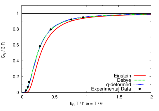
The following observations are in order.

• The horizontal curve at $\frac{C_{V}}{3R}=1$ corresponds to Dulong$-$Petit’s law of specific heat at sufficiently high temperature.

• The small filled circles correspond to experimental data points of the specific heat of Copper($Cu$) [54, 55, 56, 49].

• The blue dotted curve, which matches quite well with the experimental data point and Debye’s curve, corresponds to the specific heat variation in $q$ deformed scenario using Eq.(28). Instead of using a constant $q$-value over the wide range of temperature, we have used the temperature ($T$) dependent deformation parameter $q$, (a well known exponential decay function with $3$ free parameter, namely $q_{0},A~{}\rm{and}~{}t$)) given by (Eq.(52))

  $$q(T)=q_{0}+A\exp{(-\frac{1}{t}\frac{k_{B}T}{\hbar\omega})}$$ (29)

  with $q_{0}=1.0,A=0.08~{}\rm{and}~{}t=0.2$ (See C for the related discussion). Here $q=q_{0}=1.0$ the undeformed case; $A$ and $t$ are the parameters which can be determined for a material by fitting experimental data. Also we used numerical derivative of $q(T)$ in Eq.(28) for convenience.

• As $T\rightarrow\theta_{E}$, $q(T)\rightarrow q_{0}(=1)$ i.e. at temperature higher or above $\theta_{E}$, the fluctuation in the deformation parameter $\delta q(=q(T)-q_{0})\rightarrow 0$ can be neglected in this phenomenon of specific heat of solids.

• At other temperatures(moderate, low and very low temperatures), the curve due to $q$-deformed Einstein’s oscillators is in perfect agreement with the Debye curve and the experimental data. Note that here we considered only one single excitation mode of the oscillators (as Einstein did) and treat each atom as the $q$-deformed oscillator. This mode represents the fundamental frequency of the oscillators for a specific material. This is completely different from the Debye’s approach, in which the specific heat is viewed as the vibration of multiple excitation modes of the oscillators.

• We see that by considering only the temperature fluctuation effect(even without considering more than one mode of vibration is being triggered) we can achieve the desired result (i.e. the specific heat prediction in the $q$-deformed Einstein’s scenario matches exactly with the experimental data points) which is as good as obtained by considering the different modes of vibration as suggested by Debye.

• By fitting the experimental data for Copper(Cu) with Einstein’s theory, Debye’s theory and $q$-deformed Einstein’s theory in Fig.[1] we also found that, $\theta_{E}\sim 0.77\theta_{D}\approx 240~{}\rm{K}$ in room temperature, as $\theta_{D}=310~{}\rm{K}$ for Copper in room temperature [57]. This is consistent with the theoretical expectation $\theta_{E}\sim 0.8\theta_{D}$ [58, 59, 60].

4.2 Analysis on $q$-deformed Einstein’s theory Vs Debye’s theory

Experimental observation shows that the Debye temperature($\theta_{D}$) (which is nothing but the rescaling of the Debye frequency($\nu_{D}$) for a specific material) depends on the temperature of the material[54, 55, 61, 62]. Experimental data of the heat capacity for a specific material at very low temperature matches with the curve predicted by Debye with a higher $\theta_{D}$, whereas for the same material at room temperature, the matching requires lower value of $\theta_{D}$.

(a) $T=0\rm{-}400\rm{K}$

(b) $T=10\rm{-}70\rm{K}$

(c) $T=0\rm{-}30\rm{K}$

(d) $T=0\rm{-}15\rm{K}$

Figure 2: Variation of $C_{V}/3R$ (for $Cu$) with temperature in the Debye’s model and $q$-deformed Einstein’s model at very low temperature($0-100~{}\rm{K}$) is shown along with the experimental data points [54, 56]. The horizontal line corresponds to $C_{V}\sim 3R$.

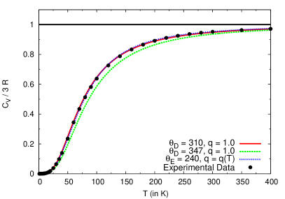
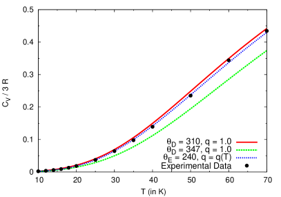
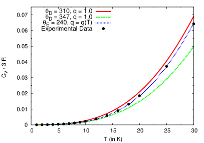
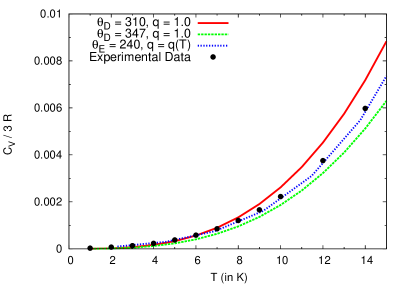
For example, at low temperature ($\sim 0~{}\rm{K}$) the values of $\theta_{D}$ for Copper(Cu) and Aluminium(Al) are $347~{}\rm{K}$ and $433~{}\rm{K}$ respectively [56, 63]; whereas, at room temperature($\sim 300~{}\rm{K}$) the values of $\theta_{D}$ for Copper(Cu) and Aluminium(Al) are $310~{}\rm{K}$ and $390~{}\rm{K}$ respectively [57]. Hence, the Debye’s temperature $\theta_{D}$ is a temperature dependent quantity i.e., $\theta_{D}=\theta_{D}(T)$.

We propose an alternate scenario(i.e., the $q$-deformed Einstein’s model, mentioned above), in which $\theta_{E}$ is assumed to be independent of the temperature. We consider the same form of $q(T)$

$$q(T)=q_{0}+A\exp{(-\frac{1}{t}\frac{k_{B}T}{\hbar\omega})}$$ (30)

which at high temperature (i.e. $T\rightarrow\infty$) goes to $1$.

In Fig.[2] we have plotted $\frac{C_{V}}{3R}$ as a function of Temperature(in K) for Copper(Cu) with $\theta_{D}=310~{}\rm{K}~{}\rm{and}~{}347~{}\rm{K}$ in Debye’s theory (using Eq.(16)) and for the $q$-deformed Einstein’s theory (using Eq.(28)) with $\theta_{E}=240~{}\rm{K}$ as well. With $q=q(T)$ Eq.(29) and (30) there is a smooth transition between the two curves and one requires the following setting of the three free parameters i.e. $q_{0}=1.0,A=0.08~{}\rm{and}~{}t=0.2$.

4.3 A comparative study of Einstein, Debye and $q$-deformed Einstein’s Theory

• Einstein model: In this model the nearest neighbour interactions between atoms are neglected and each atom vibrates with the common frequency $\nu_{E}$ i.e. the phonon (quanta of collective vibration of atoms inside the solid) frequency is assumed to be a constant, that is independent of the wave vector $k(=\frac{2\pi}{\lambda})$. The specific heat as predicted by the Einstein model matches quite well when the temperature of the solid is high (i.e. $T\gg\theta_{E}$) enough to disregard the nearest neighbour atom$-$atom interaction. It predicts the Dulong$-$Petit value $3R$ in the limit of very large $T$ (i.e $T\rightarrow\infty$). However, the model cannot explain the sufficiently low temperature behaviour of the specific heat $C_{V}\propto T^{3}$, as the model does not take care the nearest neighbour atom$-$atom interactions which need to be considered when the temperature $T$ of the solid is low. However, the model predicts $C_{V}\rightarrow 0$ as $T\ll\theta_{E}$.

• Debye model: In this model the nearest neighbour interactions between atoms are taken into consideration and each atom vibrates with a different frequency. Phonon (the quanta of the collective vibration of atoms) frequency $\omega$ is assumed to vary linearly with the wave vector $k(=\frac{2\pi}{\lambda})$($\lambda$ denotes the wavelength), i.e, $\omega=c_{s}\frac{2\pi}{\lambda}$ where $c_{s}$ is the speed of sound. The so-called Debye frequency $\omega_{D}$ is the frequency corresponding to the maximum allowed value of $\frac{2\pi}{\lambda}$ which is determined by the density of the material. The Debye spectrum is an idealization of the actual situation obtaining in a solid. For low-frequency modes (popularly known as the acoustic modes) the Debye approximation works quite well. Some reasonable discrepancies have been there in the case of high-frequency modes (named as the optical modes) [49]. At sufficiently low temperature the Debye $T^{3}$ approximation works reasonably well. This leads us to the fact that the Debye approximation is perfect when only long wavelength acoustic modes are thermally excited. On the other hand the energy of the short wavelength modes is too high for them to be populated significantly at low temperatures. As a result, $T^{3}$ approximation fails for them [50].

  Debye’s model tells us that due to interactions between each other the Einstein’s oscillators cannot retain their fundamental frequency at a given temperature; rather there will be a distribution of the frequencies of those oscillators with a maximum allowed value of the frequency.

• $q$-deformed Einstein model: Unlike the Debye’s model, where due to nearest neighbour interaction, the atomic oscillators vibrates with a wide range of frequencies (ranging from zero to the cut-off frequency $\nu_{D}$), in the $q$-deformed Einstein model, we introduce the nearest neighbour interactions in the following way(see below), however maintain the spirit of the original Einstein model. The interactions generate temperature fluctuations, which makes each of 3N Einstein oscillator $q$-deformed and is vibrating with the same angular frequency $\nu_{E}$ as in the original Einstein (undeformed) model. The specific heat $C_{V}$ dependence on the temperature $T$ is found to be in good agreement with the experimental data and also with the Debye’s result. Thus we find that even without considering more than one mode of vibration is being triggered, the model predicts the $C_{V}$ vs $T$ graph quite well and is as good as obtained by considering the different modes of vibration as suggested by Debye’s modification to the Einstein’s theory.

  In Debye’s model we have to assume the fact that the atomic oscillators vibrates with a wide range of frequencies (ranging from zero to the cut-off frequency $\nu_{D}$). Since the atom$-$atom interaction dominates over the thermal agitation at low temperature, that excites more vibration modes. Consequently in undeformed Debye model the cut-off frequency $\nu_{D}$ does not remain constant anymore, the value $\nu_{D}$ increases at very low temperature near $0~{}\rm{K}$ [56, 57, 63], which in nonextensive Tsallis scenario ($q$-deformed Einstein’s scenario) not necessarily be the case, i.e. $\nu_{E}$ can be temperature independent. Considering the effect non-equilibrium conditions which arise due to nearest neighbour atomic interaction together with temperature fluctuation at very low temperature, certain level of impurities in the sample etc., along with the unique vibration mode as suggested by Einstein, the theoretical prediction is capable to explain the experimental data points.

Approximated compact form: Eq.(28) can be converted to a more compact form using small deformation approximation(also for the time being for this purpose $q$ is to be considered as a constant approximately, i.e., not a function of temperature and $\beta^{\prime}\approx\beta$, see A), i.e., small $\mid 1-q\mid$ which states that, $e_{q}^{a}\cdot e_{q}^{b}\sim e_{q}^{a+b}$ (Eq.(35)) and $\left(e_{q}^{a}\right)^{b}\sim e_{q}^{ab}$ (Eq.(36)). Thus we find(see A, Eq.(38))

$$C_{V}=3Nk_{B}\frac{x^{2}q\left(e_{q}^{-x}\right)^{2q-1}}{\left[1-\left(e_{q}^{-x}\right)^{q}\right]^{2}}$$ (31)

For $q=1$(i.e., undeformed scenario) Eq.(31) replicates Eq.(14). Though Eq.(31) is an approximated compact analytical form of Eq.(28), it is not completely correct, as in our analysis we used $q$ as a function of temperature and also $\beta^{\prime}\approx\beta$ is not very good approximation for a wide temperature range, specially at low temperatures.

Rather we can fit the data obtained using Eq.(28) and get the specific heat of solid as a function of temperature, which is as follows

$$\frac{C_{V}}{3R}=A_{1}+\frac{A_{2}}{1+\left(\frac{x_{0}}{x}\right)^{p}}$$ (32)

with $x=\frac{\theta_{E}}{T}=\frac{h\nu_{E}}{k_{B}T}$, and the parameters $A_{1}=0.95$, $A_{2}=-0.96$, $x_{0}=4.12$ and $p=2.64$. Thus Eq.(32) can be approximated as

$$\frac{C_{V}}{3R} \approx 1-\frac{1}{1+\left(4\frac{T}{\theta_{E}}\right)^{2.7}}$$ (33)

And at very low temperature, neglecting the higher order terms in temperature we obtain

$$\frac{C_{V}}{3R}\sim 1-\left\{1-\left(4\frac{T}{\theta_{E}}\right)^{2.7}\right\}=\left(4\frac{T}{\theta_{E}}\right)^{2.7}$$ (34)

Interestingly from Eq.(34) we find that the specific heat capacity at low temperatures predicted by $q$-deformed Einstein model(nonextensive Tsallis scenario), varies nearly as $T^{3}$($\sim T^{2.7}$) which is in nice agreement with experimental observation as well as with Debye’s prediction.

5 Conclusion

We analyze the Einstein’s theory for specific heat of solid in the generalized nonextensive scenario(Tsallis statistics). We study the temperature fluctuation effect via the fluctuation in the deformation parameter $q$. At low temperature the Einstein’s curve of the specific heat in the nonextensive Tsallis scenario exactly lies on the experimental data points and matches with the Debye’s curve. Considering only the temperature fluctuation effect(even without considering more than one mode of vibration is being triggered) we can achieve the desired result (i.e. $C_{V}$ vs $T$ curve) which is as good as obtained by considering the different modes of vibration of the solid as suggested by Debye. Finally, we find, by generalizing the Einstein’s theory in nonextensive scenario(Tsallis statistics), that, a unique value of the Einstein temperature $\theta_{E}$, along with a temperature dependent deformation parameter $q(T)$, can well describe the phenomena of specific heat of solid i.e. the theory is equivalent to Debye’s theory with a temperature dependent $\theta_{D}$.

Appendix A Indicial properties of $q$-deformed exponential function for small deformation

From Eq.(4), keeping only first order in $(1-q)$,

$$e_{q}^{a}\cdot e_{q}^{b} = \left[1+(1-q)a\right]^{\frac{1}{1-q}}\cdot\left[1+(1-q)b\right]^{\frac{1}{1-q}}$$ (35)

$$= \left[1+(1-q)(a+b)+(1-q)^{2}ab\right]^{\frac{1}{1-q}}$$

$$\simeq e_{q}^{a+b}$$

Similarly, neglecting higher order terms we get,

$$\left(e_{q}^{a}\right)^{b} = \left[1+(1-q)a\right]^{\frac{b}{1-q}}$$ (36)

$$= \left[1+(1-q)ab+\frac{b(b-1)}{2!}(1-q)^{2}a^{2}+\cdots\right]^{\frac{1}{1-q}}$$

$$\approx e_{q}^{ab}$$

For constant $q$ and $\beta^{\prime}\approx\beta$, using Eqs.(35) and (36) the following approximation can be obtained for Eq.(28)

$$\frac{\sum_{n}\left(n+\frac{1}{2}\right)x\left\{e_{q}^{-\left(n+\frac{1}{2}\right)x}\right\}^{q}}{\sum_{n}\left\{e_{q}^{-\left(n+\frac{1}{2}\right)x}\right\}^{q}} \approx \frac{\sum_{n}\left(n+\frac{1}{2}\right)x\left\{e_{q}^{-nx}\right\}^{q}\left(e_{q}^{-\frac{1}{2}x}\right)^{q}}{\sum_{n}\left\{e_{q}^{-nx}\right\}^{q}\left(e_{q}^{-\frac{1}{2}x}\right)^{q}}$$ (37)

$$\approx \frac{\sum_{n}\left(n+\frac{1}{2}\right)x\left\{\left(e_{q}^{-x}\right)^{q}\right\}^{n}}{\sum_{n}\left\{\left(e_{q}^{-x}\right)^{q}\right\}^{n}}$$

$$= \frac{x}{2}\left[\frac{1+\left(e_{q}^{-x}\right)^{q}}{1-\left(e_{q}^{-x}\right)^{q}}\right]$$

Therefore Eq.(28) takes the form(for constant $q$, and $\beta^{\prime}\approx\beta$) as follows

$$\frac{C_{V}}{3R} = \frac{x}{2}\left[\frac{1+\left(e_{q}^{-x}\right)^{q}}{1-\left(e_{q}^{-x}\right)^{q}}\right]-x\frac{\partial}{\partial x}\left[\frac{x}{2}\left\{\frac{1+\left(e_{q}^{-x}\right)^{q}}{1-\left(e_{q}^{-x}\right)^{q}}\right\}\right]$$ (38)

$$= \frac{x^{2}q\left(e_{q}^{-x}\right)^{2q-1}}{\left[1-\left(e_{q}^{-x}\right)^{q}\right]^{2}}$$

Appendix B Constraints and Entropy Optimization in Tsallis Statistics

To impose the mean value of a variable in addition to satisfy the following fact

$$\int_{0}^{\infty}dx~{}p(x)=1$$ (39)

$q$-deformed mean value of a variable $x$ is to be defined as [1, 45]

$$<x>_{q}=\int_{0}^{\infty}dx~{}xP(x)=X_{q}$$ (40)

whereas, $P(x)$ is the Escort distribution and is defined as

$$P(x)=\frac{[p(x)]^{q}}{\int_{0}^{\infty}dx^{\prime}~{}[p(x^{\prime})]^{q}}$$ (41)

We immediately verify that $P(x)$ is normalized as well

$$\int_{0}^{\infty}dx~{}P(x)=\frac{\int_{0}^{\infty}dx~{}[p(x)]^{q}}{\int_{0}^{\infty}dx^{\prime}~{}[p(x^{\prime})]^{q}}=1$$ (42)

We can use these facts to optimize the generalized entropy $s_{q}$. In order to use the Lagrange’s undetermined multiplier method to find the optimized distribution we define the following quantity

$$\Phi[p]=\frac{1-\int_{0}^{\infty}dx~{}[p(x)]^{q}}{q-1}-\alpha_{q}\int_{0}^{\infty}dx~{}p(x)-\beta_{q}\frac{\int_{0}^{\infty}dx~{}x[p(x)]^{q}}{\int_{0}^{\infty}dx~{}[p(x)]^{q}}$$ (43)

with $\alpha_{q}$ and $\beta_{q}$ as the Lagrange parameters. Therefore imposing the optimization conditions

$$\frac{\partial\Phi(p)}{\partial p}=0$$ (44)

Simplifying further we get

$$p(x)=\frac{e_{q}^{-\beta_{q}\left(x-X_{q}\right)}}{\int_{0}^{\infty}dx^{\prime}~{}e_{q}^{-\beta_{q}\left(x^{\prime}-X_{q}\right)}}$$ (45)

Now from the following two constraints

• $\sum_{i}p_{i}=1$ (Norm constraint)

• $<\epsilon>_{q}=\sum_{i}\epsilon_{i}P_{i}=u_{q}$ (Energy constraint)

  with $P_{i}=\frac{p_{i}^{q}}{\sum_{j}p_{j}^{q}}$

we obtain the distribution as follows

$$p_{i}=\frac{e_{q}^{-\beta_{q}\left(\epsilon_{i}-u_{q}\right)}}{\bar{z}_{q}}$$ (46)

with $\bar{z}_{q}=\sum_{i}e_{q}^{-\beta_{q}\left(\epsilon_{i}-u_{q}\right)}$ and $\beta_{q}=\frac{\beta}{\sum_{j}p_{j}^{q}}$.

Now

$$s_{q} = k_{B}\frac{\sum_{j}p_{j}^{q}-1}{1-q}$$

$$\implies\sum_{j}p_{j}^{q} = 1+(1-q)\frac{s_{q}}{k_{B}}$$ (47)

Also

$$s_{q}=-k_{B}\ln_{q}\bar{z}_{q}=\frac{k_{B}}{1-q}\left(\bar{z}_{q}^{1-q}-1\right)$$ (48)

$$\therefore\sum_{j}p_{j}^{q}=1+(1-q)\frac{\frac{k_{B}}{1-q}\left(\bar{z}_{q}^{1-q}-1\right)}{k_{B}}=\bar{z}_{q}^{1-q}$$ (49)

So now

$$\beta_{q}=\frac{\beta}{\sum_{j}p_{j}^{q}}=\beta\bar{z}_{q}^{q-1}$$ (50)

More useful and the convenient form of Eq.(46) for application purpose, is given by [1, 45]

$$p_{i}=\frac{e_{q}^{-\beta^{\prime}\epsilon_{i}}}{Z_{q}}$$ (51)

with $Z_{q}=\sum_{i}e_{q}^{-\beta^{\prime}\epsilon_{i}}$ and $\beta^{\prime}=\frac{\beta_{q}}{1+(1-q)\beta_{q}u_{q}}=\frac{\beta}{Z_{q}^{1-q}+(1-q)\beta u_{q}}$.

Appendix C The temperature dependence of the deformation parameter $q$ in $q$-deformed Einstein’s theory)

In Fig.[3], we have plotted $\frac{C_{V}}{3R}$ as a function of $\frac{1}{x}(=\frac{T}{\theta_{E}})$ using Einstein’s theory, Debye’s modification and $q$-deformed Einstein’s theory. Here we have used some constant value of the deformation parameter $q$ in Eq.(28). In Fig.[3a] we have showed the curves for $q=1.03,1.05$, while in Fig.[3b] we set $q=1.04,1.06$.

(a) $q=1.03,1.05$

(b) $q=1.04,1.06$

Figure 3: Variation of $C_{V}/3R$ with temperature in the formalism of Einstein’s model, $q$-deformed Einstein modification is shown along with the experimental data for copper [54, 55, 56, 49].

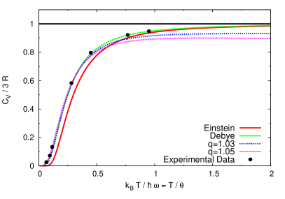
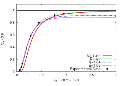
A close observation to the plots(Fig.[3]) establishes a temperature dependence of the deformation parameter $q$. We found that, for comparatively high temperature i.e., $T\rightarrow 0.5\theta~{}-~{}\theta$ the curve predicted by Debye’s theory matches with the curve obtained from small deformation(i.e., $q\sim 1.01\rm{-}1.03$) where the thermal agitation starts dominating over the atom$-$atom interaction. On the other hand at very small temperature i.e., $T\sim 0.1~{}\theta\rm{-}0.5~{}\theta$ the curve obtained from comparatively large deformation(i.e., $q\sim 1.05\rm{-}1.07$) lies on the curve predicted by Debye’s theory. For $T>\theta$, $q\rightarrow 1.0$(undeformed scenario) is enough explain the phenomena. By fitting the experimental data points for Copper(Cu) with the curves obtained from different constant value of the deformation parameter $q$, we obtain Eq.(29).

$$q(T)=q_{0}+A\exp{(-\frac{1}{t}\frac{k_{B}T}{\hbar\omega})}$$ (52)

with $q_{0}=1.0,A=0.08~{}\rm{and}~{}t=0.2$.

References

- [1] C. Tsallis, Introduction to Nonextensive Statistical Mechanics: Approaching a complex World(Springer)(2009 ).
- [2] Sumiyoshi Abe, Yuko Okamoto, Nonextensive Statistical Mechanics and Its Applications, (Lecture notes in physics ; Vol. 560), (Physics and astronomy online library), (Springer).
- [3] Ugur Tirnakli, Ernesto P. Borges, Nature, Scientific Reports 6, Article number: 23644 (2016).
- [4] Some Comments on Boltzmann-Gibbs Statistical Mechanics, Constantino Tsallis, Pergamon, Chaos, Solitons & Fractals Vol. 6, pp. 539-559, 1995, Elsevier Science Ltd.
- [5] C. Tsallis, Physica A 221 (1995) 277-290.
- [6] M. Portesi, A. Plastino, Physica A 225 (1996) 412-430.
- [7] F. Pennini, A. Plastino, A.R. Plastino, Physica A 234 (1996) 471-479.
- [8] Ugur Tlrnakh, Fevzi Buyukkilic, Dogan Demirhan, Physica A 240 (1997) 657-664.
- [9] F. Pennini, A. Plastino, A.R. Plastino, Physics Letters A 208 (1995) 309-314.
- [10] F. Buyukkilic , D. Demirhan, A. Gulec, Phys. Lett. A 197 (1995) 209.
- [11] Hugo Touchette, Christian Beck, Phys. Rev. E Stat Nonlin Soft Matter Phys. 2005 Jan;71(1 Pt 2):016131. Epub 2005 Jan 24; [arXiv:cond-mat/0408091v2] [cond-mat.stat-mech].
- [12] Christian Beck,Braz. J. Phys. vol.39 no.2a Sao Paulo Aug. 2009, [arXiv:0811.4363v2] [cond-mat.stat-mech].
- [13] Superstatistics: Recent developments and applications, Christian Beck, arXiv:cond-mat/0502306v1 [cond-mat.stat-mech].
- [14] Nonextensive statistical mechanics - Applications to nuclear and high energy physics, Constantino Tsallis and Ernesto P. Borges, (February 2, 2008) [arXiv:cond-mat/0301521v1 [cond-mat.stat-mech]].
- [15] E G D COHEN, PRAMANA Indian Academy of Sciences Vol. 64, No. 5— journal of May (2005),physics, pp. 635–643, Boltzmann and Einstein: Statistics and dynamics –An unsolved problem.
- [16] Constantino Tsallis, Brazilian Journal of Physics, vol. 29, no. 1, March, 1999, Nonextensive Statistics:Theoretical, Experimental and Computational, Evidences and Connections (1998).
- [17] A.K. Rajagopal, R.S. Mendes, E.K. Lenzi, Phys. Rev. Lett. 80 (1998) 3907.
- [18] E.K. Lenzi, R.S. Mendes, A.K. Rajagopal, Phys. Rev. E 59 (1999) 1398.
- [19] E.K. Lenzi, R.S. Mendes, A.K. Rajagopal, Physica A 286 (2000) 503–517.
- [20] C. Beck, Eur. Phys. J. A 40, 267–273 (2009).
- [21] Applications to high energy physics, Constantino Tsallis, EPJ Web of Conferences, 05001 (2011), DOI: 10.1051/epjconf/20111305001, Owned by the authors, published by EDP Sciences, 2011, Nonextensive statistical mechanics.
- [22] Constantino Tsallis, F. C. Sa Barreto, Edwin D. Loh, Phys. Rev. E, Vol. 52, No. 2 (1995).
- [23] Atanu Guha, J. Selvaganapathy and Prasanta Kumar Das, Phys. Rev. D 95, 015001 (2017).
- [24] S. Martinez, F. Nicolas, F. Pennini, A. Plastino, Physica A 286 (2000) 489–502.
- [25] C. Tsallis, J. Stat. Phys. 52 (1988) 479.
- [26] C. Tsallis, Chaos Solitons Fractals 6 (1995) 539.
- [27] J.D. Ramshaw, Phys. Lett. A 198 (1995) 119.
- [28] C. Tsallis, Phys. Lett. A 206 (1995) 389.
- [29] D. Prato, C. Tsallis, Phys. Rev. E 60 (1999) 2398.
- [30] S. Abe, A.K. Rajagopal, Phys. Rev. A 60 (1999) 3461.
- [31] A.K. Rajagopal, Phys. Rev. Lett. 76 (1996) 3469.
- [32] S. Abe, Phys. Lett. A 263 (1999) 424.
- [33] S. Abe, Eur. Phys. J. B 9 (1999) 679.
- [34] A.R. Plastino, A. Plastino, C. Tsallis, J. Phys. A 27 (1994) 5707.
- [35] C. Tsallis, Br. J. Phys. 29 (1999) 1.
- [36] A.R. Plastino, A. Plastino, Phys. Lett. A 174 (1993) 384.
- [37] V.H. Hamity, D.E. Barraco, Phys. Rev. Lett. 76 (1996) 4664.
- [38] L.P. Chimento, J. Math. Phys. 38 (1997) 2565.
- [39] B.M. Boghosian, Phys. Rev. E 53 (1996) 4754.
- [40] E.K. Lenzi, R.S. Mendes, Phys. Lett. A 250 (1998) 270.
- [41] S. Abe, Physica A 269 (1999) 403.
- [42] E.K. Lenzi, R.S. Mendes, L.R. da Silva, Physica A 280 (2000) 337.
- [43] F. Pennini, A.R. Plastino, A. Plastino, Physica A 258 (1998) 446.
- [44] A.K. Rajagopal, Sumiyoshi Abe, Phys. Rev. Lett. 83 (1999) 1711.
- [45] C. Tsallis, R. S. Mendes, A. R. Plastino, Physica A 261 (1998) 534.
- [46] T. Oikonomou, G.B. Bagci, Physics Letters A 381 (2017) 207.
- [47] A. Einstein, Annalen Physik 22 (1907) 180.
- [48] F. Reif, Fundamentals of Statistical and Thermal Physics. Waveland Press Inc., (2008), 651 p.
- [49] R. K. Pathria and P. D. Beale, Statistical Mechanics, 3rd Ed. Academic Press (2011).
- [50] Charles Kittel, Introduction to Solid State Physics, 8th Edition, John Wiley & Sons (2004).
- [51] P. Debye, Annalen der Physik 39 (1912) 789.
- [52] A. Lavagno and P. Narayana Swamy, Mod. Phys. Lett. B 13, 961 (1999); arxiv:cond-mat/0001071v1[cond-mat.stat-mech] 7 Jan 2000.
- [53] Energy distribution and energy fluctuation in Tsallis statistics, Guo Ran, Du Jiulin, arXiv:1202.0638.
- [54] G. K. White and S. J. Collocott, J. Phys. Chem. Ref. Data, Vol. 13, No. 4 (1984).
- [55] D. W. Bloom, Douglas H. Lowndes Jr., and Leonard Finegold, Review of Scientific Instruments, AIP Publishing, 41, 690 (1970); doi: 10.1063/1.1684621.
- [56] G. R. Stewart, Review of Scientific Instruments, AIP Publishing, Vol. 54, No. 1 (1983).
- [57] C. Y. Ho, R. W. Powell and P. E. Liley, Journal of Physical and Chemical Reference Data, Vol. 3, Supplement No. 1 (1974).
- [58] Solid state physics, Introduction to the thoery, James D. Patterson and Bernard C. Bailey, Springer (2007) ISBN 9780876920183.
- [59] An Introduction to Thermal Physics, Daniel V. Schroeder, Addison-Wesley, San Francisco (2000).
- [60] Terrell L. Hill, An Introduction to Statistical Mechanics, Massachusetts, U.S.A., Addison-Wesley Publishing Company (1960),ISBN 9780486652429.
- [61] P. Flubacher, A. J. Leadbetter, and J. A. Morrison, The Journal of Chemical Physics, Vol. 33, No. 6 (1960).
- [62] L. M. Shulman, A& A, 416, 187-190 (2004).
- [63] The specific heat of matter at low temperatures, A. Tari, London: Imperial College Press (2003).