Computational Motility Tracking of Calcium Dynamics in Toxoplasma gondii

Abstract.

Toxoplasma gondii is the causative agent responsible for toxoplasmosis and serves as one of the most common parasites in the world. For a successful lytic cycle, T. gondii must traverse biological barriers in order to invade host cells, and as such, motility is critical for its virulence. Calcium signaling, governed by fluctuations in cytosolic calcium (Ca²⁺) concentrations, is utilized universally across life and regulates many cellular processes, including the stimulation of T. gondii virulence factors, such as motility. Therefore, increases in cytosolic Ca²⁺, called calcium oscillations, serve as a means to link and quantify the intracellular signaling processes that lead to T. gondii motility. Here, we describe our work extracting, quantifying, and modeling motility patterns of T. gondii before and after Ca²⁺ stimulation via the addition of pharmacological drugs and/or extracellular calcium. We demonstrate a computational pipeline including a robust tracking system using optical flow and dense trajectory features to extract T. gondii motility patterns. Using this pipeline, we were able to track T.gondii motility dynamics in response to cytosolic Ca²⁺ fluxes in extracellular parasites. This allows us to study how Ca²⁺ signaling via release from intracellular Ca²⁺ stores and/or from extracellular Ca²⁺ entry relates to motility patterns, a crucial first step in developing countermeasures for T. gondii virulence.

1. Introduction

Cellular motility serves as a fundamental and core characteristic shared across life, with key molecular components conserved across protozoa, bacteria, and vertebrates. Within cellular biology directional motility is an essential process involved in embryonic development, wound healing, neurology, T-cell immune response, and tissue development (Pollard and Borisy, 2003). Toxoplasma gondii is the causative agent of disseminated toxoplasmosis. T. gondii is capable of infecting virtually any nucleated cell, making it the most prolific of all parasitic infections. Infections are lifelong and the immunocompromised are at particularly high risk due to reactivation of dormant tissue cysts that can lead to complications such as encephalitis, myocarditis, ocular toxoplasmosis, and congenital transmission. Calcium signaling is utilized universally across life, as binding of Ca²⁺ to signaling effectors induces a cascade of downstream processes. Fluxes in basal cytosolic Ca²⁺ levels ([Ca²⁺]_i) serve as the basis for signaling, as mechanisms to either rapidly increase or decrease cytosolic Ca²⁺ levels are intricately balanced. Calcium signaling has been shown to stimulate every step of the T. gondii lytic cycle, comprised of egress, gliding motility, invasion, and replication. Nevertheless, little is known about the molecules and mechanism involved in Ca²⁺ signaling in T. gondii. Egress, gliding motility, and invasion all require activation of the molecular machinery involved in generating the mechanical force needed for progression throughout the lytic cycle. This activation is achieved either directly or indirectly via secondary signaling messangers, orginating from upstream Ca²⁺ mediated processes. Unfortunately, the exact sequence and identity of the signaling molecules involved in T. gondii Ca²⁺ signaling are unknown (Wang et al., 2015)(Borges-Pereira et al., 2015).

To elucidate the connection between Ca²⁺ signaling and its effects on T. gondii motility, we propose a novel motility tracking algorithm. Using this algorithm, we can track Ca²⁺ dynamics in extracellular parasites in order to determine how changes induced by Ca²⁺ signaling relate to motility patterns of invasive T. gondii. Ideally, our work will help us identify differences between mammalian Ca²⁺ signaling and parasite Ca²⁺ signaling for future drug targets, shedding further light on the eventual development of countermeasures against T. gondii virulence.

The impetus for this research was to design a robust tracking system capable of tracking and quantifying induced motility changes of T. gondii parasites in response to Ca²⁺ signaling. Object tracking, the process of locating a moving object in video data, has been employed in a variety of applications, including human-computer interaction, security, surveillance, video communication, augmented reality, traffic control, medical imaging, and video editing (Mountney et al., 2010). Numerous examples of video tracking exist in biology and neuroscience literature, including an automated tracking and segmentation framework by Hue-Fang et al. (Yang and Choe, 2009), a mathematical approach for cell tracking, through formulating the cell tracking problem which is proposed by Blazakis et al., (Blazakis et al., 2014) and blood cell tracking using Hough transform model and fuzzy curve tracing (Kiratiratanapruk and Sinthupinyo, 2012).

Motility is a fundamental process across both unicellular and multicellular organisms, filling a critical role in processes such as cancer progression, embryonic development, immune response, and tissue development. Cellular homeostasis involves responding to numerous constantly changing environmental cues such as ionic composition or signaling compounds. Such stimuli induce the intracellular signaling pathways needed to activate the molecular machinery for generation of mechanical force. Thus, cellular motility is key to proper cellular homeostasis and development, and the molecules and mechanisms involved in the signaling events are of great interest (Becker et al., 2005). For these reasons, we examined the motility of T. gondii and propose a robust tracking algorithm for the ultimate purpose of using eventual motility models to design therapeutic countermeasures.
Here, we proposed an algorithm to track and statistically analyze Ca²⁺ signaling-induced motility events and corresponding changes in motility patterns of T. gondii. Toxoplasmosis is a disease caused by the T. gondii parasite. Infections of toxoplasmosis are usually asymptomatic in healthy adults, and are characterized by occasional mild flu-like symptoms such as muscle aches and tender lymph nodes. In a small number of people, eye problems may develop. In those with a weak immune system severe symptoms such as seizures and poor coordination may occur. If infected during pregnancy, a condition known as congenital toxoplasmosis may affect the child and lead to still-born death (Wang et al., 2015). These disease pathologies of T. gondii motivate the need for an accurate and robust method for analyzing the source of T. gondii virulence: its motility.

We propose a Ca²⁺ signaling-induced motility analysis model as described below. First, we developed a robust video tracker to identify and track T. gondii parasites. Then we extracted the necessary statistics together with the spatial trajectories of the parasites. The purpose of the trajectories is to describe the motion path of the parasites.

2. Method

In this section, we discuss the methodology of our proposed computational pipeline.

2.1. Data

We recorded fluorescence microscopy videos of Ca²⁺ dynamics of T. gondii expressing a genetically encoded calcium indicator (GCaMP6f). In the presence of increased cytosolic Ca²⁺, the indicator increases in fluorescence, allowing us to track Ca²⁺ dynamics across the lytic cycle. Videos are acquired using a LSM 710 confocal microscope in a heated chamber set to $37^{\circ}$C. 35 mm glass bottom cover dishes (MATTEK) were treated with 2 mL of 10% FBS (Fetal Bovine Serum) in PBS (Phosphate Buffer Solution) pH 7.4 overnight at $4^{\circ}$C. The following morning excess FBS was washed with PBS. Freshly egressed parasites expressing GCaMP6f were collected, purified, and resuspended in 1 mL of Ringer Buffer without calcium.  2.5 x 10⁷ parasites were loaded onto cover dishes using a cell culture cylinder and incubated for approximately 15 min on ice to allow for cells to adhere. After removing the cell culture cylinder, Ringer Buffer was added to a 2 ml final volume. [11]

2.2. Software

We implemented the pipeline in Python 2.7, including libraries such as Numpy, Scipy, and Matplotlib for optimized linear algebra computations and visualizations. The core of our tracking algorithm used a combination of tools available in the OpenCV 3.1 computer vision library. The full code for our pipeline is openly available under the MIT open source license at https://github.com/quinngroup/toxoplasma

2.3. Computational Pipeline

Our pipeline is illustrated in Fig. 1. Broadly, we imported the videos, preprocessed them, and extracted the motility statistics, and parasite trajectories using two different trackers. With the manual tracking approach, we extracted the motility, intensity, and velocity of specific, manually-identified objects. In both cases, trajectories were extracted using optical flow analysis. After importing video data, we proceed with the following preprocessing steps:

$\bullet$ Step 1::

Apply gamma correction and logarithmic correction on one level of tracking to increase the chance of object recognition.

$\bullet$ Step 2::

Apply erosion and dilation after creating binary images to remove false negatives and false positives for each frame. Additionally, thinning the edges to distinguish any cells clumped together.

$\bullet$ Step 3::

Apply a localized histogram transformation to remove background hue.

In the next step, we designed two trackers to follow individual parasites and link them to Ca²⁺ oscillations. First, we started with a manual tracker: a baseline approach that followed the current state-of-the-art in T. gondii Ca²⁺-induced motility tracking. We then implemented a variant of the KLT tracker (Amini et al., 2014) to follow all the parasite objects in a given video simultaneously.

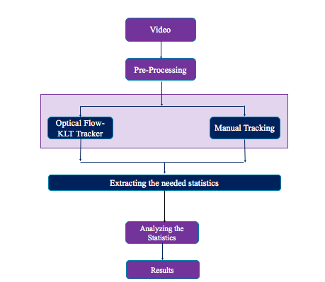
Figure 1. Ca²⁺-signaling induced motility tracking pipeline.

2.3.1. Manual Tracker

The manual tracker requires tracking two versions of the data at once: grayscale and binarized levels. This is due to the fact that intensity serves as a direct correlation to cellular Ca²⁺ levels, in addition to the fluorescent T. gondii parasites themselves. In our videos the cells expressing the genetically encoded Ca²⁺ indicator initially appear dim green, but after increases in cytosolic calcium via extracellular Ca²⁺ addition or addition of pharmacological drugs, causes the indicator to increase its fluorescence. Therefore, the intensity of each cell can be used to track calcium oscillations, and serves as the main factor we have to measure in relating Ca²⁺ signaling to T. gondii virulence. Additionally, we track the motility patterns of the T. gondii parasites themselves, in particular to observe the differences in motility before and after calcium stimulation.

There are numerous disadvantages to a manual tracker in this context. First, the cells are abnormally shaped (banana-shaped) and undergo affine transformations throughout the video, making them difficult to follow using static shape templates. Second, they can move in and out of the focal plane of the microscope, causing the tracker to lose them. Third, minor oscillations in fluorescence, irrespective of external Ca²⁺ addition or drug stimulation, causes the tracker to lose the objects.

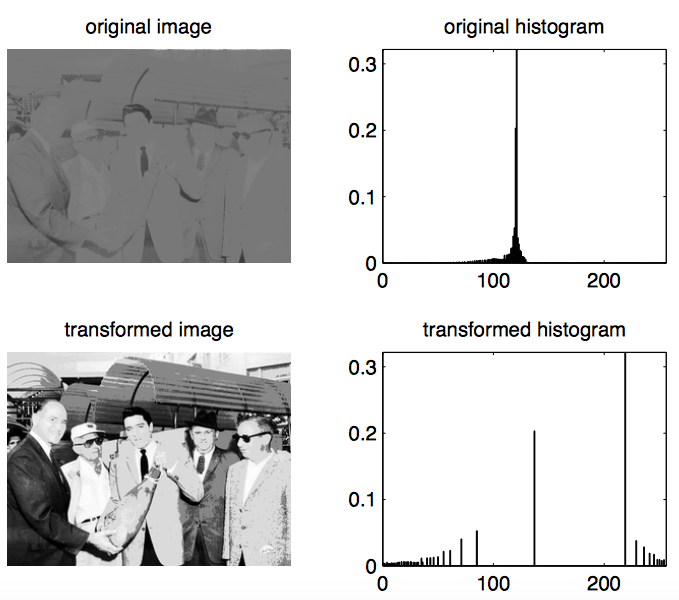
Figure 2. Effect of localized histogram method applied on a sample image[6].

To cope with these issues, we improved the algorithm in two steps. First, we applied some preprocessing operations like gamma correction and logarithmic correction. In this case, even if an object has a very low intensity we can recover it from the background. Then, we applied histogram localizations to remove background noise. In some cases, the background includes some green hue which may cause some noise. To eliminate this background noise, we used local histogram equalization.

Local histogram equalization(Ketcham et al., 1974) is a technique for adjusting image intensities to enhance contrast. It differs from ordinary histogram equalization in the respect that the adaptive method computes several histograms, each corresponding to a distinct section of the image, and uses them to redistribute the lightness values of the image. It is, therefore, suitable for improving the local contrast and enhancing the definitions of edges in each region of an image (Ketcham et al., 1974). The application of this method is demonstrated in Fig. 2.

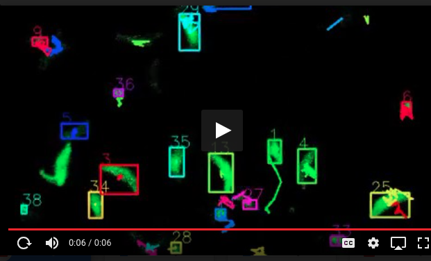
Figure 3. A snapshot of final manual tracking of T. gondii parasites.

After applying the preprocessing steps to each frame, we find the contours of each parasite for each frame, assign a bounding box to each contour, and find the closest object spatially from the previous frame. These two objects are then considered the same object across subsequent frames. A representative image of our tracking module is illustrated in Fig. 3. We also establish parameters to handle objects that move out of frame or too which move too quickly to be tracked. For the latter, if the relative centers of the two aligned objects across frames are spatially separate beyond a certain threshold, they remain as two distinct objects to our tracker. For the former, when an object disappears, we record the position of disappeared object and wait a certain number of frames to see if it reappears. As with the object alignment, we place a hard threshold on the wait time; beyond that threshold we consider the object lost. After developing our manual tracking algorithm, we measured the velocity, average distance traveled, and intensity of each tracked parasite. By considering the cells separately we measured three kinds of motions and the intensities of each cell. For velocity computation, we considered the pixels which are passed in each subsequent frame. The details are illustrated in Fig. 4.

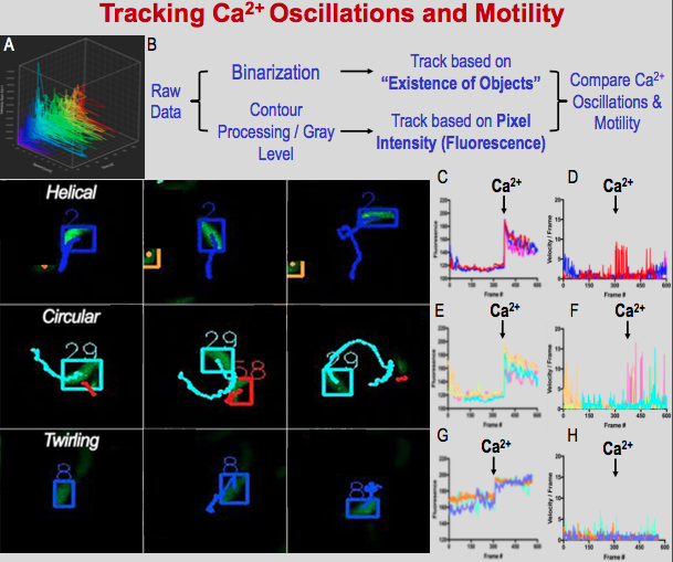
Figure 4. Manual Tracking Result A) Calcium Oscillations vs. Time vs. Speed. B) Scheme for Tracking method. C) Representative images of motility types using new tracking module. C) Helical Ca²⁺ Oscillations Fluorescence Tracings D) Helical Velocity Tracks E) Circular Fluorescence Ca²⁺ Oscillations F) Circular Motility Velocity Tracks G) Twirling Ca²⁺ Oscillations Tracings H) Twirling Ca²⁺ Velocity Tracks

2.3.2. KLT Tracker

Although our manual tracking algorithm is an improvement over that which was used in T. gondii Ca²⁺-induced motility assessment, we still needed a tracking approach robust enough to overcome some of the more common shortcomings of the manual tracker, such as parasite depth occlusions and alignment problems across frames. For this reason the KLT tracker was a good alternative to apply for our purposes. (Tomasi and Kanade, 1991) The Lucas-Kanade tracker (KLT) uses the Tomasi algorithm to find fixed points. KLT makes use of the spatial intensity information to direct the search for the position that yields the best match. It is faster than traditional techniques for examining far fewer potential matches between images. In this approach, we consider some features extracted through the Tomasi algorithm of the object, which are fed to the KLT and tracked over the course of the video.(Aires et al., 2008) The resulting tracker is very robust against the kinds of failure modes we observed in our manual tracker (Fig. 5).

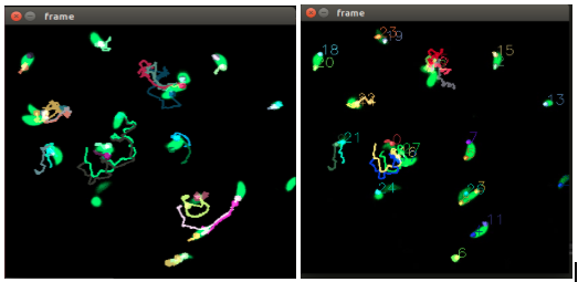
Figure 5. Cell tracking result using KLT (left) and the same result by allocating numbers to each point (right)

3. Results

We extracted trajectories from our manual tracking and the KLT implementation. Our findings are as follows. In Fig. 6 we observed all trajectories extracted from a sample video in a 2D space. Fig. 7 links this information with cytosolic Ca²⁺ oscillations, as indicated by the shade of the plot (brighter hue representing higher Ca²⁺ levels). From this, we are able to observe how the motility patterns of T. gondii parasites abruptly change in the presence of extracellular Ca²⁺, clearly implying a causal relationship.

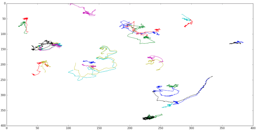
Figure 6. 2D plot of all cell trajectory using KLT (x and y axis are showing the coordinates of each point during the time)

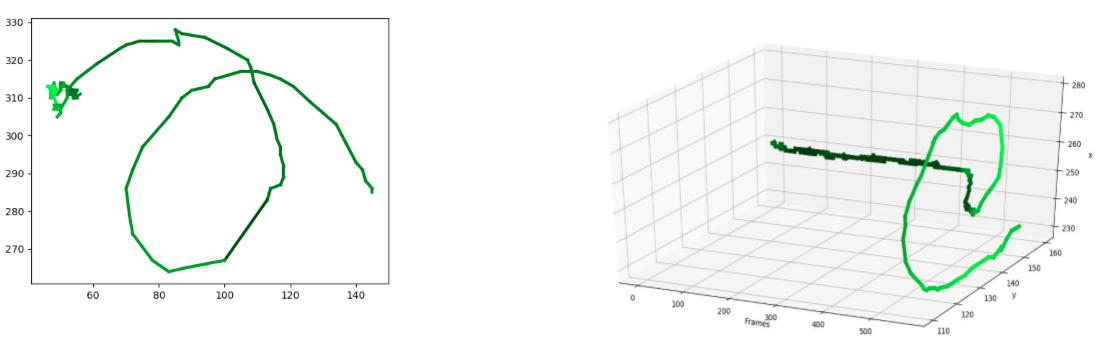
Figure 7. 2D plot of a sample cell trajectory with intensity and 3D representation of another sample object (left). On the right, the trajectory is colored to indicate the level of fluorescence of the tracked parasite. From this, it is easy to see when the Ca²⁺ signaling was added to the system.

3.1. Extracted statistics

As a means to evaluate the robustness of our tracking algorithm against our hypothesis, we extracted the X and Y coordinates of a single motile cell. This approach enables us to generate several pieces of statistical data related to motility, such as the translational and angular velocity, as indicated in Figures. 8 and 9. Our cells exhibit multiple types of motility that relate to movement within a coordinate plane (helical and circular), thus it is necessary to compute both the translational and angular velocity, respectively. Furthermore, we can interpret how the fluorescence (cytosolic Ca²⁺ concentration), as indicated by the shade of the green hue of the line plot, relates to burst or dips in speed post addition of Ca²⁺ or drug stimulation.

3.1.1. Object Calcium Levels

Levels of Ca²⁺ are indicated by the intensity of fluorescence of the tracked parasites. To compute the Ca²⁺ levels by way of intensity, for each point we considered a $nxn$ rectangle, while the coordination of the point is located at the center of that rectangle. Then we calculated the average intensity of all non-zero pixels located inside of the rectangle. The reason of considering a $nxn$ window instead of just one point intensity is clear: each point may be in the border of the object or even out of the object but attached to that object. Thus, by considering the intensity in a $nxn$ window we have better estimation of intensity value of an object.

3.1.2. Object Velocities

Object velocities were computed in two steps. First, we computed the instantaneous velocity of each object per pair of consecutive frames. To do this we needed to know the distance between 2 consecutive time points:

$P1=(x1,y1)$ and $P2=(x2,y2)$ (1)

Where $P1$ and $P2$ are the coordinates of an object across two consecutive frames. Thus, the distance between these two points is calculated through a simple Euclidean distance formula:

$$d=\sqrt{(x_{1}-x_{2})^{2}+(y_{1}-y_{2})^{2}}\textbf{ (2) }$$

$$v=\frac{d}{\Delta t}\textbf{ (3) }$$

since we are going to check the velocity of each object per frame, we have $t=1$. Thus, we can use the formula (2) as a metric to compute the instantaneous velocity. In the next step, we smooth the instantaneous velocities with a sliding window. Our results in computing instantaneous and smoothed velocities are shown in Fig. 8.

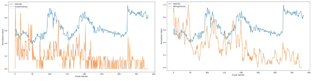
Figure 8. 2D plot of a sample cell intensity VS. Instantaneous velocity (left) and the averaged sliding velocity (right)

3.1.3. Objects Angular Velocities

Angular velocity is an important component to understanding the instantaneous motility dynamics of T. gondii, as our cells tend to move in counterclockwise circular patterns. To compute the angular velocity, we need to know the object orientation or object angle per frame, and we can calculate it as:

$$\theta=\arctan(\frac{y}{x})\textbf{ (4) }$$

where $y$ and $x$ are the coordinates of point $P$ in frame $T$. Thus after computing the angles of all points in all frames, we can easily compute the Angular velocity which is defined as follows:

$$\textit{Angular Velocity}=\theta_{2}-\theta_{1}\textbf{ (5) }$$

Where $\theta_{1}$ and $\theta_{2}$ are angle values of an object in $2$ consecutive frames. Thus, the differences between two angles in two consecutive frames shows instantaneous angular velocity. To obtain the sliding average angular velocity we should compute as done previously.

The significance of this metric is because of the fact that it can show the randomness of movements before calcium addition (if any random movement existed) and non-random motility after calcium addition. To compute the angle histogram, we should use the following formula:

$$\theta=\arctan(\frac{y_{2}-y_{1}}{x_{2}-x_{1}})\textbf{ (6) }$$

A representative plot of the instantaneous and sliding angular velocity using our tracking module is seen in Fig. 9.

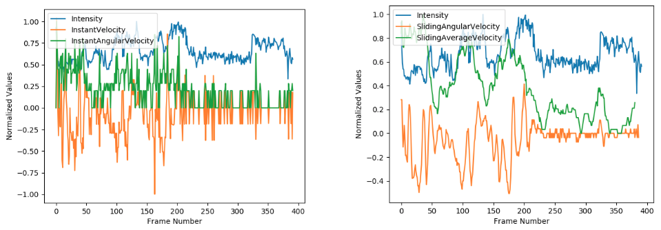
Figure 9. 2D plot of a sample cell intensity VS Instantaneous velocity and Instantaneous angular velocity (left) and the averaged sliding velocity and averaged sliding angular velocity(right)

4. Discussion

Trajectories play a crucial role in our work because we can follow the dynamics of cell motility across them. The pipeline presented here successfully identifies the three known motility types (Fig. 10). Part $A$ of Fig. 10 shows the motility types and the trajectories of three selected parasites found to be following each type. In part $B$,$C$, and $D$ of this figure one can see a $4D$ representations of each cell trajectory. These dimensions include $X$ and $Y$ coordinates, frame number, and the intensity of a representative cell track across consecutive frames as shown by the hue of the trajectory curve. The hue intensity represents the calcium levels of a single cell and is used as a proxy for $Ca^{2+}$ oscillations. At approximately the $350^{th}$ frame one can see an increase in the green hue as it becomes brighter, due to the addition of extracellular $Ca^{2+}$. Afterwards, one see the cell begin to move. It is important to highlight that increases in calcium (brighter hue coloring of the line) are linked to increases in motility ( a change in the $X$-$Y$ coordinates of the line).

From the XY coordinates we can extrapolate several pieces of information and relate them to the fluorescence signal (Ca²⁺ level). If one looks at Fig. 10, part E indicates the calcium oscillation patterns for other similar objects undergoing the same type of motility as portrayed in their representative column. After the addition of Ca²⁺, the fluorescence intensity is increased dramatically, as indicated by the addition of extracellular calcium around Frame 350 and appears to cause the cells to oscillate in a somewhat coordinated frequency and amplitude pattern. The most interesting finding is illustrated in Fig. 10 part H, where one can see the Ca²⁺ oscillations plotted together with the velocity across time, as peaks in normalized average velocity and normalized averaged angular velocity correlate with peaks of cytosolic Ca²⁺. As it is clear in Fig. 10, most of the time, there is a direct relationship between changes in fluorescence intensity and the object translational and angular velocity. Moreover, if one looks at this part again he or she will see the addition of 2 kinds of reagents that are applied in 2 different points of the time - Thapsigargin (TG) (pharmacological reagent that causes increased levels of cytosolic Ca²⁺ and extracellular Ca²⁺) - . What we discovered and found it extremely interesting was the effect of those two drugs on motility pattern; at the beginning the intensity is changing randomly, as a consequence the velocity and the angular velocity are also changing stochastically. Then by adding TG we will see the random oscillation of intensity is paused, causing the intensity, the object velocity, and the angular velocity to appear more stable - after addition of TG and before addition of Ca²⁺ -. Finally by addition of Ca²⁺ , the intensity is increased sharply and after a short delay phase both the velocities are increased considerably. To highlight this phenotype in more detail we isolated and plotted the tracks within their own separate figure (Fig. 11). There on the left side of the figure, before addition of TG, the intensity is fluctuating randomly but by addition of TG around the 300th frame, then the intensity level becomes more stable. Again, we can see that by addition of Ca²⁺ at approximately the 400th frame, the intensity increases greatly. In the meantime, the translational velocity and angular velocity are shown on the right side of the figure. They show the same behavior as the intensity shows in front of TG and Ca²⁺ addition. Another interesting point is in the right side of the figure is at the frame 600, where, both the angular velocity and translational velocities increase dramatically a few seconds after reaching the max value of intensity caused by calcium stimulation.

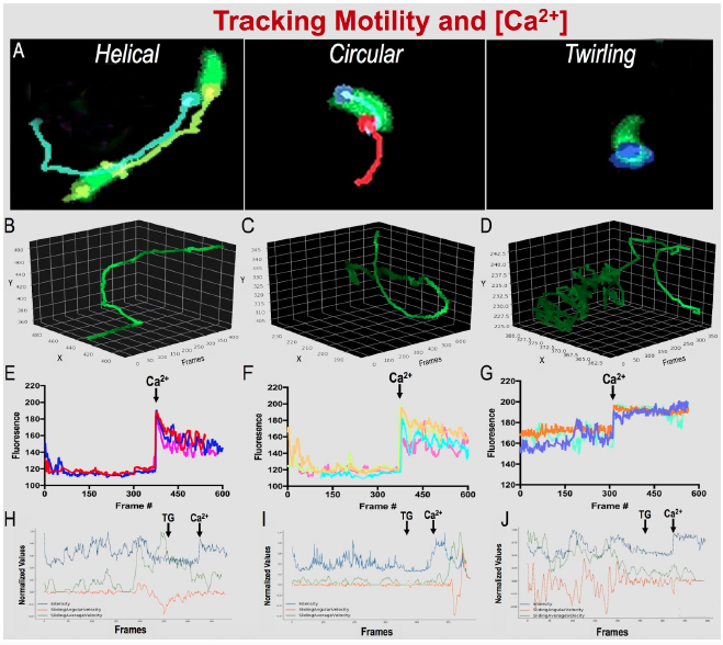
Figure 10. A) Representative images of motility types using tracking module. B,C and D ) 4D plot of X and Y coordinates, Frame number, and fluorescence intensity ( line hue color ) of helical, circular, and Twirling motility, respectively. E,F, G) Ca²⁺ Oscillations Fluorescence Tracing of Helical, Circular and Twirling motility, respectively. H, I, and J ) Ca²⁺Fluorescence Tracing versus Translation velocity versus Angular velocity of Helical, Circular, and Twirling motility respectively.

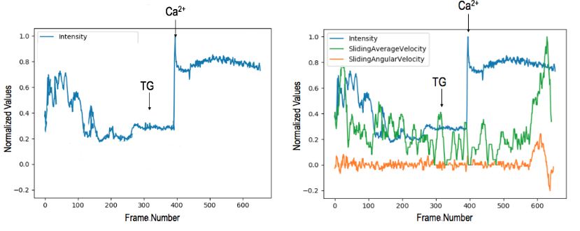
Figure 11. left : The intensity-time plot of a specific cell , Right : the intensity vs translational velocity vs angular velocity. in both the sides the interesting points of TG and Ca²⁺ are indicated.

Fig. 12, shows those interesting points in a circular motility trajectory. This 4D representation from time view indicates The Ca²⁺ addition point and TG addition point.

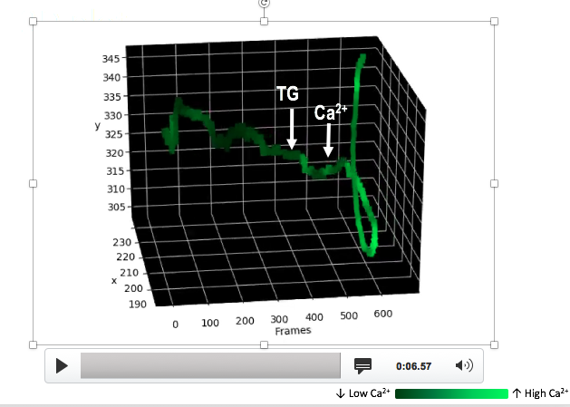
Figure 12. left : demonstration of TG and Ca²⁺ addition points on a 4D representation of a cell trajectory.

In addition, to see the interesting findings in an entire video, we depict all objects trajectories in a 4D view (Fig. 13) . This view, enables us to understand more of the effect of TG and Ca²⁺ . Moreover, As it is obvious at the same figure, after addition of calcium all the trajectories are much brighter than previous time which shows us the amount of calcium is increasing after calcium addition in all the cells.

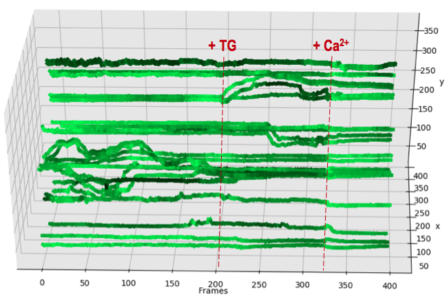
Figure 13. Time-View demonstration of TG and Ca²⁺ addition points on a 4D representation of all cell trajectories.

5. Generalizing the pipeline for big data and other types of trajectories

In theory our framework’s ability to track, analyze, and classify the motility dynamics of $Toxoplasma$ $gondii$ is readily applicable to related species of motile parasites, including $Plasmodium$ ookinetes and sporozoites that undergo similar motility patterns. However, our pipeline was designed from the ground-up with T. gondii as it main applicant, and these are only initial results; there are numerous important applications of motility tracking throughout public health that would benefit from this framework, and we anticipate the application of this platform will be significantly useful to solve those problems. In order for our pipeline to be effectively applied to another organism, parameters such as the number frames recorded per second, the pixel size, the number of frames used for averaging speed, or determining angular velocity have to be carefully tested and optimized.

In our current application, the question is not simply a matter of vast amount of video data. Videos of T. gondii motility are expensive to create and acquire. It requires fully-staffed labs with a lot of time to grow the parasites, plate them, and image them over periods of time. Hence, right now, the data-generation step is not scalable. Thus, we are not yet at the point of being able to say that the our video data are massive.

However, in the future, we anticipate a scalable analysis framework in which by rewriting the code in a distributed fashion (for instance, since our pipeline is written by python we can use easily PySpark or Flink) and managing the data we can generalize our algorithm to be robust on big data. To do that, first the videos would be analyzed in parallel to extract trajectories, then the trajectories would be stacked onto a tall-and-skinny matrix that is row-distributed. In this matrix, each column and each row of a matrix correspond, respectively, to one object and one video frame. in each row, we measure the objects location ( X and Y value of objects ) and intensity value of the objects in that specific frame. So, here the objects are features and the rows are the observations of those features. Since the number of objects is quite fewer than the number of the frames we will have a tall and skinny matrix of trajectories. In the next step, each trajectory could either be analyzed in parallel on its respective node, or we can perform distributed matrix decomposition on the matrix.

Generally speaking, our challenge with the big data would be rearrangement of distributed operations through Spark, Flink or Dask that can smoothly process each video chunk on HDFS and extract the desired statistics, exactly like what we have done previously on large scale FMRI images(Li et al., 2016).

6. Conclusion

Here, we developed a KLT-based tracker and compared it to manual tracking of Ca²⁺-induced T. gondii motility patterns. We shown that, how we extracted the data and statistics from trajectory. For future work, we already planned to capture the motions using dense trajectories. dense trajectories are the dense version of optical flow (Wang et al., 2011) - despite the KLT which is the sparse version of optical flow - . So, We then study the trajectories by clustering them and applying machine learning techniques to categorize them. In doing so, we gain a deeper understanding of the possible motion types of T. gondii under different environmental stimuli and, therefore, an avenue through which to understand the virulence factors of T. gondii.

References

- (1)
- Aires et al. (2008) Kelson RT Aires, Andre M Santana, and Adelardo AD Medeiros. 2008. Optical flow using color information: preliminary results. In Proceedings of the 2008 ACM symposium on Applied computing. ACM, 1607–1611.
- Amini et al. (2014) Amineh Amini, Hadi Saboohi, Teh Ying Wah, and Tutut Herawan. 2014. A fast density-based clustering algorithm for real-time internet of things stream. The Scientific World Journal 2014 (2014).
- Becker et al. (2005) Wayne M Becker, Lewis J Kleinsmith, and Jeff Hardin. 2005. The world of the cell. Benjamin-Cummings Publishing Company.
- Blazakis et al. (2014) KN Blazakis, CC Reyes-Aldasoro, V Styles, C Venkataraman, and A Madzvamuse. 2014. An optimal control approach to cell tracking. (2014).
- Borges-Pereira et al. (2015) Lucas Borges-Pereira, Alexandre Budu, Ciara A McKnight, Christina A Moore, Stephen A Vella, Miryam A Hortua Triana, Jing Liu, Celia RS Garcia, Douglas A Pace, and Silvia NJ Moreno. 2015. Calcium Signaling throughout the Toxoplasma gondii Lytic Cycle A STUDY USING GENETICALLY ENCODED CALCIUM INDICATORS. Journal of Biological Chemistry 290, 45 (2015), 26914–26926.
- Ketcham et al. (1974) David J Ketcham, Roger W Lowe, and J William Weber. 1974. Image enhancement techniques for cockpit displays. Technical Report. HUGHES AIRCRAFT CO CULVER CITY CA DISPLAY SYSTEMS LAB.
- Kiratiratanapruk and Sinthupinyo (2012) Kantip Kiratiratanapruk and Wasin Sinthupinyo. 2012. Worm egg segmentation based centroid detection in low contrast image. In Communications and Information Technologies (ISCIT), 2012 International Symposium on. IEEE, 1139–1143.
- Li et al. (2016) Xiang Li, Milad Makkie, Binbin Lin, Mojtaba Sedigh Fazli, Ian Davidson, Jieping Ye, Tianming Liu, and Shannon Quinn. 2016. Scalable fast rank-1 dictionary learning for fmri big data analysis. In Proceedings of the 22nd ACM SIGKDD International Conference on Knowledge Discovery and Data Mining. ACM, 511–519.
- Mountney et al. (2010) Peter Mountney, Danail Stoyanov, and Guang-Zhong Yang. 2010. Three-dimensional tissue deformation recovery and tracking. IEEE Signal Processing Magazine 27, 4 (2010), 14–24.
- Pollard and Borisy (2003) Thomas D Pollard and Gary G Borisy. 2003. Cellular motility driven by assembly and disassembly of actin filaments. Cell 112, 4 (2003), 453–465.
- Tomasi and Kanade (1991) Carlo Tomasi and Takeo Kanade. 1991. Detection and tracking of point features. (1991).
- Wang et al. (2011) Heng Wang, Alexander Kläser, Cordelia Schmid, and Cheng-Lin Liu. 2011. Action recognition by dense trajectories. In Computer Vision and Pattern Recognition (CVPR), 2011 IEEE Conference on. IEEE, 3169–3176.
- Wang et al. (2015) Shuai Wang, Chunwei Lan, Luwen Zhang, Haizhu Zhang, Zhijun Yao, Dong Wang, Jingbo Ma, Jiarong Deng, and Shiguo Liu. 2015. Seroprevalence of Toxoplasma gondii infection among patients with hand, foot and mouth disease in Henan, China: a hospital-based study. Infectious diseases of poverty 4, 1 (2015), 53.
- Yang and Choe (2009) Huei-Fang Yang and Yoonsuck Choe. 2009. Cell tracking and segmentation in electron microscopy images using graph cuts. In Biomedical Imaging: From Nano to Macro, 2009. ISBI’09. IEEE International Symposium on. IEEE, 306–309.