Ibadan Lectures on Toric Varieties

Abstract.

These notes are based on, and significantly extend, Frank Sottile’s short course of four lectures at the CIMPA school on Combinatorial and Computational Algebraic Geometry in Ibadan, Nigeria that took place 12–23 June 2017.

Toric varieties are perhaps the most accessible class of algebraic varieties. They often arise as varieties parameterized by monomials, and their structure may be completely understood through objects from geometric combinatorics. While accessible and understandable, the class of toric varieties is also rich enough to illustrate many properties of algebraic varieties. Toric varieties are also ubiquitous in applications of mathematics, from tensors to statistical models to geometric modeling to solving systems of equations, and they are important to other branches of mathematics such as geometric combinatorics and tropical geometry.

For additional reference, see [5, 9, 10, 13] (the last is freely accessible and covers some material from the perspective of real toric varieties). For an accessible background on algebraic geometry and Gröbner bases, we recommend [4], which is a classic and won the American Mathematical Society’s Leroy P. Steele Prize for Exposition in 2016 [1].

Notation and a note about our field

We write ${\mathbb{C}}$ for the complex numbers, ${\mathbb{R}}$ for the real numbers, ${\mathbb{Q}}$ for the rational numbers, ${\mathbb{Z}}$ for the integers, and ${\mathbb{N}}$ for the natural numbers (nonnegative integers). While we describe complex toric varieties, the description holds verbatim for any field as toric varieties are naturally schemes over $\mbox{spec}({\mathbb{Z}})$. When the ambient field $\Bbbk$ is not algebraically closed, there is an attractive theory of arithmetic toric varieties [8].

1. Affine Toric Varieties

Recall that every finitely generated free abelian group $G$ is isomorphic to ${\mathbb{Z}}^{m}$ for some positive integer $m$ called the rank of $G$, and the isomorphism is equivalent to choosing a basis for $G$.

Write ${\mathbb{C}}^{*}$ for the group of nonzero complex numbers and $({\mathbb{C}}^{*})^{n}$ for the complex torus of invertible diagonal $n\times n$ complex matrices, equivalently, of ordered $n$-tuples of nonzero complex numbers. The free abelian group ${\mathbb{Z}}^{n}$ of rank $n$ is associated to $({\mathbb{C}}^{*})^{n}$ in two distinct ways. It is isomorphic to the lattice of one-parameter subgroups ${\mbox{\rm Hom}_{g}}({\mathbb{C}}^{*},({\mathbb{C}}^{*})^{n})$ of group homomorphisms from ${\mathbb{C}}^{*}$ to $({\mathbb{C}}^{*})^{n}$. These are also called cocharacters. An integer vector $w=(w_{1},\dotsc,w_{n})\in{\mathbb{Z}}^{n}$ gives the map which sends $t\in{\mathbb{C}}^{*}$ to the diagonal matrix ${t^{w}}:=\operatorname{\rm diag}(t^{w_{1}},\dotsc,t^{w_{n}})\in({\mathbb{C}}^{*})^{n}$. The group of characters, $\mbox{\rm Hom}_{g}(({\mathbb{C}}^{*})^{n},{\mathbb{C}}^{*})$, equivalently of Laurent monomials, is also isomorphic to ${\mathbb{Z}}^{n}$. Here, an integer vector $a=(a_{1},\dotsc,a_{n})^{T}\in{\mathbb{Z}}^{n}$ gives the Laurent monomial ${x^{a}}:=x_{1}^{a_{1}}\dotsb x_{n}^{a_{n}}$, which is also a group homomorphism $({\mathbb{C}}^{*})^{n}\ni x\mapsto x^{a}\in{\mathbb{C}}^{*}$, where $x=\operatorname{\rm diag}(x_{1},\dotsc,x_{n})$.

This ambiguity in the two roles for ${\mathbb{Z}}^{n}$ is resolved by writing $N$ for the cocharacters and $M$ for the characters. When expressed as integer vectors, elements of $N$ will be row vectors and those of $M$ column vectors. Applying a character $a\in M$ to a cocharacter $w\in N$ gives a character of ${\mathbb{C}}^{*}$, which is an integer, well-defined up to sign. A standard choice gives the standard Euclidean pairing $N\otimes M\to{\mathbb{Z}}$, which we may see by computing

$$(t^{w})^{a}\ =\ (t^{w_{1}})^{a_{1}}\dotsb(t^{w_{n}})^{a_{n}}\ =\ t^{w_{1}a_{1}+\dotsb+w_{n}a_{n}}\ =\ t^{w\cdot a}\,.$$

The coordinate ring of $({\mathbb{C}}^{*})^{n}$ is the ring ${\mathbb{C}}[x_{1},x_{1}^{-1},\dotsc,x_{n},x_{n}^{-1}]$ of Laurent polynomials. This is also the group algebra ${\mathbb{C}}[M]$ and we write ${\mathbb{C}}[x^{\pm}]$ for this Laurent ring.

1.1. Affine Toric Varieties

Let ${{\mathcal{A}}}\subset M\simeq{\mathbb{Z}}^{n}$ be a finite subset of monomials/characters. It is convenient to represent ${\mathcal{A}}$ as the set of column vectors of an integer matrix with $n$ rows. We will also write ${\mathcal{A}}$ for this matrix. We will use this set ${\mathcal{A}}$ to index coordinates, variables, etc. For example $({\mathbb{C}}^{*})^{\mathcal{A}}$ is the set of functions from ${\mathcal{A}}$ to ${\mathbb{C}}^{*}$. It is the algebraic torus $({\mathbb{C}}^{*})^{|{\mathcal{A}}|}$ whose coordinates are indexed by the elements of ${\mathcal{A}}$. Likewise ${\mathbb{C}}^{\mathcal{A}}$ is the vector space of functions from ${\mathcal{A}}$ to ${\mathbb{C}}$. It has coordinates $(z_{a}\mid a\in A)$. If ${\mathcal{A}}$ is represented by the matrix $(\begin{smallmatrix}0&0&1&1\\ 0&1&0&1\end{smallmatrix})$, then ${\mathbb{C}}^{\mathcal{A}}\simeq{\mathbb{C}}^{4}$ has coordinates $z_{(\mbox{\tiny$\begin{smallmatrix}0\\ 0\end{smallmatrix}$})}$, $z_{(\mbox{\tiny$\begin{smallmatrix}0\\ 1\end{smallmatrix}$})}$, $z_{(\mbox{\tiny$\begin{smallmatrix}1\\ 0\end{smallmatrix}$})}$, $z_{(\mbox{\tiny$\begin{smallmatrix}1\\ 1\end{smallmatrix}$})}$.

This set ${\mathcal{A}}$ may be used to define a map ${\varphi_{\mathcal{A}}}\colon({\mathbb{C}}^{*})^{n}\to{\mathbb{C}}^{\mathcal{A}}$, where

(1.1) $$\varphi_{\mathcal{A}}(x)\ :=\ (x^{a}\mid a\in{\mathcal{A}})\,.$$

In the example where ${\mathcal{A}}$ is represented by the matrix $(\begin{smallmatrix}0&1&0&1\\ 0&0&1&1\end{smallmatrix})$, for $(x,y)\in({\mathbb{C}}^{*})^{2}$, $\varphi_{\mathcal{A}}(x,y)=(1,x,y,xy)\in{\mathbb{C}}^{\mathcal{A}}$. Notice that the map $\varphi_{\mathcal{A}}$ (1.1) is a group homomorphism $\varphi_{\mathcal{A}}\colon({\mathbb{C}}^{*})^{n}\to({\mathbb{C}}^{*})^{\mathcal{A}}$ followed by the inclusion $({\mathbb{C}}^{*})^{\mathcal{A}}\hookrightarrow{\mathbb{C}}^{\mathcal{A}}$. The Zariski closure of the image $\varphi_{\mathcal{A}}(({\mathbb{C}}^{*})^{n})$ in ${\mathbb{C}}^{\mathcal{A}}$ is the affine toric variety $X_{\mathcal{A}}$. We deduce two characterizations of affine toric varieties from this definition. Affine toric varieties are varieties that arise as the closure in ${\mathbb{C}}^{m}$ of a subtorus of $({\mathbb{C}}^{*})^{m}$, and affine toric varieties are varieties that are parameterized by monomials. Note that the torus $({\mathbb{C}}^{*})^{n}$ acts on $X_{\mathcal{A}}$ with a dense orbit and this action extends to the ambient affine space ${\mathbb{C}}^{\mathcal{A}}$.

If the subgroup ${\mathbb{Z}}{\mathcal{A}}$ of $M$ generated by ${\mathcal{A}}$ is a proper subgroup, then the homomorphism $\varphi_{\mathcal{A}}$ has a nontrivial kernel ${T}:=\ker\varphi_{\mathcal{A}}$. In this case, $\varphi_{\mathcal{A}}$ (1.1) induces an injective map on $({\mathbb{C}}^{*})^{n}/T\to{\mathbb{C}}^{\mathcal{A}}$. In Exercise 1, you are asked to verify these claims and identify the kernel. We have that ${\mathbb{Z}}{\mathcal{A}}$ is the lattice of characters of $({\mathbb{C}}^{*})^{n}/T$ and so $\dim X_{\mathcal{A}}=\dim({\mathbb{C}}^{*})^{n}/T=\operatorname{\rm rank}{\mathbb{Z}}{\mathcal{A}}$.

Example 1.1.

Suppose that $n=1$ and ${\mathcal{A}}=\{2,3\}\subset{\mathbb{Z}}$. For $s\in{\mathbb{C}}^{*}$, $\varphi_{\mathcal{A}}(s)=(s^{2},s^{3})\in{\mathbb{C}}^{2}$. The closure of $\varphi_{\mathcal{A}}(({\mathbb{C}}^{*})^{n})$ is the cuspidal cubic, ${\mathcal{V}}(y^{2}-x^{3})$, where ${\mathbb{C}}^{2}$ has coordinates $(x,y)$:

Since ${\mathbb{Z}}{\mathcal{A}}={\mathbb{Z}}$, $\varphi_{\mathcal{A}}$ is injective. This may also be seen as if $(x,y)=\varphi_{\mathcal{A}}(s)$, then $s=y/x$.

Suppose that $k,m\geq 1$ are integers. Let ${\mathbf{e}}_{1},\dotsc,{\mathbf{e}}_{k}$ and ${\mathbf{f}}_{1},\dotsc,{\mathbf{f}}_{m}$ be the standard unit basis vectors for ${\mathbb{Z}}^{k}$ and ${\mathbb{Z}}^{m}$, respectively, and set

$${\mathcal{A}}\ :=\ \{{\mathbf{e}}_{i}+{\mathbf{f}}_{j}\mid i=1,\dotsc,k\mbox{ and }j=1,\dotsc,m\}\subset{\mathbb{Z}}^{k}\times{\mathbb{Z}}^{m}\,,$$

which has $mn$ elements. The map $\varphi_{\mathcal{A}}\colon{\mathbb{C}}^{k}\times{\mathbb{C}}^{m}\to{\mathbb{C}}^{km}$ is

$$(x_{1},\dotsc,x_{k}\,,\,y_{1},\dotsc,y_{m})\ \longmapsto\ (x_{i}y_{j}\mid i=1,\dotsc,k\mbox{ and }j=1,\dotsc,m)\,.$$

If ${\mathbb{C}}^{km}$ is identified with the space of $k\times m$ matrices, this map is $(x,y)\mapsto xy^{T}$, and thus $X_{\mathcal{A}}$ is the space of $k\times m$ matrices of rank at most 1.

Finally, suppose that $d\geq 1$ is an integer. The $d$th Veronese map $\varphi_{\mathcal{A}}\colon{\mathbb{C}}^{n}\to{\mathbb{C}}^{\binom{d+n}{n}}$, is when ${\mathcal{A}}$ is the set of all exponent vectors in ${\mathbb{N}}^{n}$ of degree at most $d$. When $n=1$ and $d=3$, we have ${\mathcal{A}}=\{0,1,2,3\}\subset{\mathbb{Z}}$ and $\varphi_{\mathcal{A}}(x)=(1,x,x^{2},x^{3})$. Ignoring the first coordinate which is constant, $X_{\mathcal{A}}$ is the moment (rational normal) curve in ${\mathbb{C}}^{3}$.

1.2. Toric Ideals

The ideal $I_{\mathcal{A}}$ of $X_{\mathcal{A}}$ is a toric ideal. It is an ideal of the coordinate ring ${\mathbb{C}}[z_{a}\mid a\in{\mathcal{A}}]$ of the affine space ${\mathbb{C}}^{\mathcal{A}}$. To understand $I_{\mathcal{A}}$, consider the pullback map corresponding to $\varphi_{\mathcal{A}}$ on coordinate rings,

$${\varphi^{*}_{\mathcal{A}}}\ \colon\ {\mathbb{C}}[z_{a}\mid a\in{\mathcal{A}}] \longrightarrow {\mathbb{C}}[x_{1},x_{1}^{-1},\dotsc,x_{n},x_{n}^{-1}]$$

$$z_{a}\mbox{\qquad} \longmapsto \mbox{\qquad}x^{a}\ .$$

The toric ideal $I_{\mathcal{A}}$ is the kernel of $\varphi^{*}_{\mathcal{A}}$. The exponent of a monomial $z^{u}$ in ${\mathbb{C}}[z_{a}\mid a\in{\mathcal{A}}]$ is the vector $u=(u_{a}\mid a\in{\mathcal{A}})\in{\mathbb{N}}^{\mathcal{A}}$, and the image of $z^{u}$ under $\varphi^{*}_{\mathcal{A}}$ is

$$\varphi^{*}_{\mathcal{A}}(z^{u})\ =\ \prod_{a\in{\mathcal{A}}}(x^{a})^{u_{a}}\ =\ x^{\sum au_{a}}\,.$$

Let us write the sum $\sum_{a\in{\mathcal{A}}}au_{a}$ in this exponent as ${\mathcal{A}}u$. When ${\mathcal{A}}$ is represented by an integer matrix ${\mathcal{A}}$, this is the usual matrix-vector product. Observe that the kernel $I_{\mathcal{A}}$ of $\varphi^{*}_{\mathcal{A}}$ contains the following set of binomials

(1.2) $$\{z^{u}-z^{v}\mid{\mathcal{A}}u={\mathcal{A}}v\}\,.$$

Suppose that ${\mathcal{A}}$ is represented by the matrix $(\begin{smallmatrix}0&1&2&3&4\\ 4&3&2&1&0\end{smallmatrix})$. If $u=(0,1,1,1,0)^{T}$ and $v=(1,0,1,0,1)^{T}$, then ${\mathcal{A}}u={\mathcal{A}}v$, which gives the binomial in $I_{\mathcal{A}}$,

$$z_{(\mbox{\tiny$\begin{smallmatrix}1\\ 3\end{smallmatrix}$})}z_{(\mbox{\tiny$\begin{smallmatrix}2\\ 2\end{smallmatrix}$})}z_{(\mbox{\tiny$\begin{smallmatrix}3\\ 1\end{smallmatrix}$})}\ -\ z_{(\mbox{\tiny$\begin{smallmatrix}0\\ 4\end{smallmatrix}$})}z_{(\mbox{\tiny$\begin{smallmatrix}2\\ 2\end{smallmatrix}$})}z_{(\mbox{\tiny$\begin{smallmatrix}4\\ 0\end{smallmatrix}$})}\,.$$

Theorem 1.2.

The toric ideal $I_{\mathcal{A}}$ is a prime ideal. As a complex vector space, it is spanned by the binomials (1.2).

Proof.

The image of $\varphi^{*}_{\mathcal{A}}$ is the subalgebra of ${\mathbb{C}}[x^{\pm}]$ generated by the monomials $\{x^{a}\mid a\in{\mathcal{A}}\}$. Since ${\mathbb{C}}[x^{\pm}]$ is a domain, the kernel $I_{\mathcal{A}}$ is a prime ideal. An equivalent way to see this is to note that $X_{\mathcal{A}}$ is irreducible (hence its coordinate ring is a domain and its defining ideal is prime) as $X_{\mathcal{A}}$ is the closure of the image of the irreducible variety $({\mathbb{C}}^{*})^{n}$ under the map $\varphi_{\mathcal{A}}$.

For the second statement, let $\prec$ be any term order on ${\mathbb{C}}[z_{a}\mid a\in{\mathcal{A}}]$. Let $f\in I_{\mathcal{A}}$. We may write $f$ as

$$f\ =\ c_{u}z^{u}\ +\ \sum_{v\prec u}c_{v}z^{v}\qquad c_{u}\neq 0\,,$$

so that $\mbox{\rm in}_{\prec}(f)=c_{u}z^{u}$ is the initial term of $f$. Then

$$0\ =\ \varphi^{*}_{\mathcal{A}}(f)\ =\ c_{u}x^{{\mathcal{A}}u}\ +\ \sum_{v\prec u}c_{v}x^{{\mathcal{A}}v}\ .$$

There is some $v\prec u$ with ${\mathcal{A}}v={\mathcal{A}}u$, for otherwise the term $c_{u}x^{{\mathcal{A}}u}$ is not canceled in $\varphi^{*}_{\mathcal{A}}(f)$ and $\varphi^{*}_{\mathcal{A}}(f)\neq 0$. Set $\overline{f}:=f-c_{u}(z^{u}-z^{v})$. Then $\varphi^{*}_{\mathcal{A}}(\overline{f})=0$ and $\mbox{\rm in}_{\prec}(\overline{f})\prec\mbox{\rm in}_{\prec}(f)$.

If the leading term of $f$ were $\prec$-minimal in the initial ideal $\mbox{\rm in}_{\prec}(I_{\mathcal{A}})$, then $\overline{f}$ would be zero, and so $f$ is a scalar multiple of a binomial of the form (1.2). Suppose now that $\mbox{\rm in}_{\prec}f$ is not minimal in $\mbox{\rm in}_{\prec}(I_{\mathcal{A}})$ and that every polynomial in $I_{\mathcal{A}}$ all of whose terms are $\prec$-less than the initial term of $f$ is a linear combination of binomials of the form (1.2). Then $\overline{f}$ is a linear combination of binomials of the form (1.2), which implies that $f$ is as well, by our induction hypothesis. This completes the proof.

A monoid has an associative binary operation and an identity element, but it does not necessarily have inverses. (A semigroup only has an associative binary operation, and not necessarily an identity.) While many authors use the adjective semigroup when working with toric varieties, the identification below of maximal ideals with monoid homomorphisms shows the inadequacy of that language. Note that the complex numbers under multiplication forms a monoid and any group is also a monoid. Define ${\mathbb{N}}{\mathcal{A}}$ to be the submonoid of $M$ generated by ${\mathcal{A}}$. It consists of all linear combinations of elements of ${\mathcal{A}}$ whose coefficients are natural numbers. Write ${\mathbb{C}}[{\mathbb{N}}{\mathcal{A}}]$ for the monoid algebra, which is the set of complex-linear combinations of elements of ${\mathbb{N}}{\mathcal{A}}$. It is also the set of Laurent polynomials whose exponents are from ${\mathbb{N}}{\mathcal{A}}$.

Corollary 1.3.

The coordinate ring of the affine toric variety $X_{\mathcal{A}}$ is ${\mathbb{C}}[{\mathbb{N}}{\mathcal{A}}]$.

Proof.

The map $\sum_{a\in{\mathcal{A}}}an_{a}\mapsto\prod_{a\in{\mathcal{A}}}(x^{a})^{n_{a}}$ is a bijection between the submonoid ${\mathbb{N}}{\mathcal{A}}$ and the monoid of monomials $(x^{a}\mid a\in{\mathcal{A}})$ generated by ${\mathcal{A}}$. In the proof of Theorem 1.2, we identified the coordinate ring ${\mathbb{C}}[X_{\mathcal{A}}]$ of $X_{\mathcal{A}}$ with the subring of ${\mathbb{C}}[x^{\pm}]$ generated by the monomials $\{x^{a}\mid a\in{\mathcal{A}}\}$, which is the monoid algebra ${\mathbb{C}}[{\mathbb{N}}{\mathcal{A}}]$ by the identification of ${\mathbb{N}}{\mathcal{A}}$ with the monomials in ${\mathbb{C}}[X_{\mathcal{A}}]$.

Theorem 1.2 gives an infinite generating set for $I_{\mathcal{A}}$. We seek more economical generating sets. Suppose that ${\mathcal{A}}u={\mathcal{A}}v$ with $u,v\in{\mathbb{N}}^{\mathcal{A}}$. We define vectors $r,w^{\pm}$. For $a\in{\mathcal{A}}$, set

$${r_{a}} := \min(u_{a},v_{a})\,,$$

$${w^{+}_{a}} := \max(u_{a}-v_{a},0)\,,\quad\mbox{and}$$

$${w^{-}_{a}} := \max(v_{a}-u_{a},0)\,.$$

Then $w^{+},w^{-}\in{\mathbb{N}}^{\mathcal{A}}$ and we have $u-v=w^{+}-w^{-}$ with $u=r+w^{+}$ and $v=r+w^{-}$, and so

(1.3) $$z^{r}(z^{w^{+}}-z^{w^{-}})\ =\ z^{u}-z^{v}\ \in\ I_{\mathcal{A}}\,,$$

with $z^{r}=\gcd\{z^{u},z^{v}\}$. Note also that ${\mathcal{A}}w^{+}={\mathcal{A}}w^{-}$ as $0={\mathcal{A}}(u-v)={\mathcal{A}}(w^{+}-w^{-})$, so that $z^{w^{+}}-z^{w^{-}}\in I_{\mathcal{A}}$. In our example where ${\mathcal{A}}=(\begin{smallmatrix}0&1&2&3&4\\ 4&3&2&1&0\end{smallmatrix})$, we have $r=(0,0,1,0,0)^{T}$, $w^{+}=(0,1,0,1,0)^{T}$ and $w^{-}=(1,0,0,0,1)^{T}$, and

$$z_{(\mbox{\tiny$\begin{smallmatrix}1\\ 3\end{smallmatrix}$})}z_{(\mbox{\tiny$\begin{smallmatrix}2\\ 2\end{smallmatrix}$})}z_{(\mbox{\tiny$\begin{smallmatrix}3\\ 1\end{smallmatrix}$})}\ -\ z_{(\mbox{\tiny$\begin{smallmatrix}0\\ 4\end{smallmatrix}$})}z_{(\mbox{\tiny$\begin{smallmatrix}2\\ 2\end{smallmatrix}$})}z_{(\mbox{\tiny$\begin{smallmatrix}4\\ 0\end{smallmatrix}$})}\ =\ z_{(\mbox{\tiny$\begin{smallmatrix}2\\ 2\end{smallmatrix}$})}\bigl{(}z_{(\mbox{\tiny$\begin{smallmatrix}1\\ 3\end{smallmatrix}$})}z_{(\mbox{\tiny$\begin{smallmatrix}3\\ 1\end{smallmatrix}$})}\ -\ z_{(\mbox{\tiny$\begin{smallmatrix}0\\ 4\end{smallmatrix}$})}z_{(\mbox{\tiny$\begin{smallmatrix}4\\ 0\end{smallmatrix}$})}\bigr{)}\ \in\ I_{\mathcal{A}}\,.$$

For $u\in{\mathbb{Z}}^{\mathcal{A}}$, let $u^{+}$ be the coordinatewise maximum of $u$ and the $0$-vector, and let $u^{-}$ be the coordinatewise maximum of $-u$ and the $0$-vector.

Corollary 1.4.

$I_{\mathcal{A}}=\langle z^{u^{+}}-z^{u^{-}}\mid{\mathcal{A}}u=0\rangle$.

Thus $I_{\mathcal{A}}$ is generated by binomials coming from the integer kernel of the matrix ${\mathcal{A}}$.

Theorem 1.5.

Any reduced Gröbner basis of $I_{\mathcal{A}}$ consists of binomials.

The point of this theorem is that Buchberger’s algorithm is binomial-friendly. That is, if $f$ and $g$ are binomials, then their $S$-polynomial is again a binomial, and the reduction of one binomial by another is again a binomial. You are asked to prove Theorem 1.5 in Exercise 7.

It is an important problem to compute or to find relatively small Gröbner bases for toric ideals. By Corollary 1.4, these are given by special subsets of the integer kernel $\{u\in{\mathbb{Z}}^{\mathcal{A}}\mid{\mathcal{A}}u=0\}$ of ${\mathcal{A}}$. For example, a reduced Gröbner basis for the ideal of $k\times m$ matrices of rank 1 is given by

$$\{\underline{z_{a,b}z_{c,d}}-z_{a,d}z_{c,b}\mid 1\leq a<c\leq k\mbox{ and }1\leq b<d\leq m\}\,,$$

where the term order is the degree reverse lexicographic order with the variables ordered by $z_{a,b}\prec z_{c,d}$ if $a<c$ or $a=c$ and $b>d$ (the leading term is underlined). This is the set of all $2\times 2$ minors of the $k\times m$ matrix $(z_{ij})_{i=1,\dotsc,k}^{j=1,\dotsc,m}$ of indeterminates.

By Corollary 1.3, the coordinate ring of the toric variety $X_{\mathcal{A}}$ is the algebra ${\mathbb{C}}[{\mathbb{N}}{\mathcal{A}}]\simeq{\mathbb{C}}[x^{a}\mid a\in{\mathcal{A}}]$. This subalgebra of the ring ${\mathbb{C}}[x^{\pm}]={\mathbb{C}}[M]$ of Laurent polynomials is spanned by monomials. Let us generalize this. Given a finitely generated submonoid $S$ of $M$ (this is a subset of $M$ that contains $0$ and is closed under addition), write ${{\mathbb{C}}[S]}\subset{\mathbb{C}}[x^{\pm}]$ for the monoid algebra of $S$. This is the set of all complex-linear combinations of elements of $S$, where the multiplication is distributive and induced by the monoid operation of $S$. Choosing a generating set ${\mathcal{A}}$ of $S$, so that $S={\mathbb{N}}{\mathcal{A}}$, realizes ${\mathbb{C}}[S]$ as the coordinate ring of the affine toric variety $X_{\mathcal{A}}\subset{\mathbb{C}}^{\mathcal{A}}$. Then the usual algebraic-geometry dictionary implies that

$$X_{\mathcal{A}}\ =\ \operatorname{\rm spec}({\mathbb{C}}[{\mathbb{N}}{\mathcal{A}}])\,.$$

Thus $\operatorname{\rm spec}({\mathbb{C}}[S])$ is an affine toric variety without a preferred embedding into affine space. Under the algebraic-geometry dictionary, the closed points $X_{\mathcal{A}}({\mathbb{C}})$ of $X_{\mathcal{A}}$ correspond to the maximal ideals of ${\mathbb{C}}[{\mathbb{N}}{\mathcal{A}}]$.

There is a second perspective on these points, via monoid homomorphisms. By Exercise 9, maximal ideals correspond to monoid homomorphisms $\mbox{\rm Hom}_{m}(S,{\mathbb{C}})$, from $S$ to ${\mathbb{C}}$ (additive on $S$ and multiplicative on ${\mathbb{C}}$). An element ${\mathfrak{m}}$ of $\mbox{\rm Hom}_{m}(S,{\mathbb{C}})$ is a function ${\mathfrak{m}}\colon S\to{\mathbb{C}}$ such that ${\mathfrak{m}}(0)=1$ and for $a,b\in S$, ${\mathfrak{m}}(a+b)={\mathfrak{m}}(a)\cdot{\mathfrak{m}}(b)$.

The map $\varphi_{\mathcal{A}}$ (1.1) restricts to the real torus ${({\mathbb{R}}^{*})^{n}}\subset({\mathbb{C}}^{*})^{n}$ and gives a map $\varphi_{\mathcal{A}}\colon({\mathbb{R}}^{*})^{n}\to{\mathbb{R}}^{\mathcal{A}}$. The closure of the image is the real affine toric variety $X_{\mathcal{A}}({\mathbb{R}})$. If we write ${\mathbb{R}}_{>}$ for the positive real numbers and ${\mathbb{R}}_{\geq}$ for the nonnegative real numbers, then we may also restrict $\varphi_{\mathcal{A}}$ to ${\mathbb{R}}^{n}_{>}$. Note that $\varphi_{\mathcal{A}}({\mathbb{R}}^{n}_{>})\subset{\mathbb{R}}_{\geq}^{\mathcal{A}}$, the positive orthant in ${\mathbb{R}}^{\mathcal{A}}$. The nonnegative affine toric variety $X_{{\mathcal{A}},\geq}$ is the closure of the image. We have the following maps

(1.4) $$X_{{\mathcal{A}},\geq}\ \lhook\joinrel\relbar\joinrel\relbar\joinrel\rightarrow\ X_{\mathcal{A}}({\mathbb{R}})\ \lhook\joinrel\relbar\joinrel\relbar\joinrel\rightarrow\ X_{\mathcal{A}}({\mathbb{C}})\ \relbar\joinrel\twoheadrightarrow\ X_{{\mathcal{A}},\geq}\ .$$

These are induced by the maps

(1.5) $${\mathbb{R}}_{\geq}\ \lhook\joinrel\relbar\joinrel\relbar\joinrel\rightarrow\ {\mathbb{R}}\ \lhook\joinrel\relbar\joinrel\relbar\joinrel\rightarrow\ {\mathbb{C}}\ \relbar\joinrel\twoheadrightarrow\ {\mathbb{R}}_{\geq}\,,$$

with the last map $z\mapsto|z|$. The maps (1.4) also come from the identification of affine toric varieties with monoid homomorphisms and the sequence of maps of monoids (1.5). As the composition of these monoid maps is the identity, the composition (1.4) is also the identity.

Exercises

1. Show that the monomial map $\varphi_{\mathcal{A}}\colon({\mathbb{C}}^{*})^{n}\to({\mathbb{C}}^{*})^{\mathcal{A}}$ (1.1) is injective if and only if ${\mathcal{A}}$ generates $M$. When ${\mathcal{A}}$ does not generate $M$, identify the kernel of $\varphi_{\mathcal{A}}$.

2. Let $n\in{\mathbb{N}}$ be a natural number. Describe generators of the toric ideal $I_{\mathcal{A}}$ for the point set ${\mathcal{A}}=\left(\begin{matrix}0&1&2&3&\cdots&n\end{matrix}\right)$. Do the same for the point set ${\mathcal{A}}=(\begin{smallmatrix}0&1&2&\cdots&n\\ n&\cdots&2&1&0\end{smallmatrix})$.

3. Breakfast Problem. Suppose that ${\mathcal{A}}\subset{\mathbb{Z}}^{4}$ is represented by the $4\times 8$ matrix

   $$\left(\begin{matrix}1&1&1&1&1&1&1&1\\ 1&1&1&1&0&0&0&0\\ 1&1&0&0&1&1&0&0\\ 1&0&1&0&1&0&1&0\end{matrix}\right)\ .$$

   Find a set of nine linearly independent generators of the toric ideal $I_{\mathcal{A}}$.

4. Let ${\mathcal{A}}\subset{\mathbb{Z}}^{6}=({\mathbb{Z}}^{2})^{3}$ be represented by the $6\times 8$ matrix

   $$\left(\begin{matrix}1&1&1&1&0&0&0&0\\ 0&0&0&0&1&1&1&1\\ 1&1&0&0&1&1&0&0\\ 0&0&1&1&0&0&1&1\\ 1&0&1&0&1&0&1&0\\ 0&1&0&1&0&1&0&1\end{matrix}\right)\ .$$

   Find linearly independent generators of the toric ideal $I_{\mathcal{A}}$. Hint: The even (respectively odd) numbered rows give the vertices of the $3$-cube. What is $X_{\mathcal{A}}$? For this, consider the map $\varphi_{\mathcal{A}}$ where the rows correspond to the variables $x_{0},x_{1},y_{0},y_{1},z_{0},z_{1}$ and the columns to the variables $p_{000},p_{100},\dotsc,p_{111}$.

5. Show that the collection of $2\times 2$ minors of the $k\times m$ matrix $(z_{ij})_{i=1,\dotsc,k}^{j=1,\dotsc,m}$ of indeterminates forms a reduced Gröbner basis for the toric ideal of the variety $X_{\mathcal{A}}$ of matrices of rank 1, where the term order is degree reverse lexicographic with the variables ordered by $z_{a,b}\prec z_{c,d}$ if $a<c$ or $a=c$ and $b>d$. What about other term orders?

6. Identify a generating set and a reduced Gröbner basis for the toric ideal $I_{\mathcal{A}}$ given by as many of the following six subsets of ${\mathbb{Z}}^{2}$ as you can. The origin is at the lower left of each figure. You may find computer software useful.

                                 

7. Work out the details of the suggested proof of Theorem 1.5. Explain why ‘reduced’ is necessary for the conclusion.

8. A submonoid $S\subset M$ is saturated if for any $a\in M$ and $k\in{\mathbb{N}}$ with $k\neq 0$, if $ka\in S$, then $a\in S$. Show that if ${\mathbb{C}}[S]$ is normal, then $S$ is saturated. Can you prove the converse of this statement?

9. Let $S$ be a finitely generated submonoid of $M$. Show that every maximal ideal ${\mathfrak{m}}$ of ${\mathbb{C}}[S]$ restricts to a monoid homomorphism from $S$ to ${\mathbb{C}}$, and vice-versa. Hint: use that maximal ideals correspond to algebra maps ${\mathbb{C}}[S]\to{\mathbb{C}}$.

10. For ${\mathcal{A}}\subset M$ finite, show that $X_{\mathcal{A}}({\mathbb{R}})=\mbox{\rm Hom}_{m}({\mathbb{N}}{\mathcal{A}},{\mathbb{R}})$ and $X_{{\mathcal{A}},\geq}=\mbox{\rm Hom}_{m}({\mathbb{N}}{\mathcal{A}},{\mathbb{R}}_{\geq})$.

11. Use the embedding $x\mapsto(x,x^{-1})$ of the torus ${\mathbb{C}}^{*}$ into ${\mathbb{C}}^{2}$, or any other method, to identify the coordinate ring of the torus ${\mathbb{C}}^{*}$ with ${\mathbb{C}}[x,x^{-1}]$. Deduce that the coordinate ring of $({\mathbb{C}}^{*})^{n}$ may be identified with ${\mathbb{C}}[x_{1},x_{1}^{-1},\dotsc,x_{n},x_{n}^{-1}]$. Show that this is the complex group ring ${\mathbb{C}}[M]$ of the free abelian group $M$ of characters of the torus $({\mathbb{C}}^{*})^{n}$. Harder: Can you relate algebraic structures of ${\mathbb{C}}[M]$ to the group structure on $({\mathbb{C}}^{*})^{n}$? That is, what do the product, inverse, and identity element of $({\mathbb{C}}^{*})^{n}$ correspond to on ${\mathbb{C}}[M]$ and $M$.

2. Toric Projective Varieties and Solving Equations

Some affine toric varieties may be considered to be projective varieties—this is when they are stable under the multiplication by scalars on their ambient vector space. In this case, they have particularly attractive properties. Such projective toric varieties also provide a means to prove one of the signature results related to toric varieties; Kushnirenko’s Theorem about the number of solutions to a system of sparse polynomial equations.

2.1. Toric Varieties in Projective Space

Projective space ${{\mathbb{P}}^{m}}={{\mathbb{P}}({\mathbb{C}}^{m+1})}$ is the set of one-dimensional linear subspaces of ${\mathbb{C}}^{m+1}$. Since a one-dimensional linear subspace $\ell$ is generated by any nonzero point of $\ell$, and scalar multiplication by elements of ${\mathbb{C}}^{*}$ acts simply transitively on these nonzero points of $\ell$, and freely on ${\mathbb{C}}^{m+1}\smallsetminus\{0\}$, we may identify ${\mathbb{P}}^{m}$ with the quotient $({\mathbb{C}}^{m+1}\smallsetminus\{0\})/{\mathbb{C}}^{*}$. Projective space is equipped with homogeneous coordinates $[z_{0}:\dotsb:z_{m}]$, were we identify $[z_{0}:z_{1}:\dotsb:z_{m}]$ with $[tz_{0}:tz_{1}:\dotsb:tz_{m}]$ for any nonzero scalar $t\in{\mathbb{C}}^{*}$. An affine variety $X\subset{\mathbb{C}}^{m+1}$ corresponds to a projective variety in ${\mathbb{P}}({\mathbb{C}}^{m+1})={\mathbb{P}}^{m}$ when $X$ is homogeneous under the ${\mathbb{C}}^{*}$-action on ${\mathbb{C}}^{m+1}$ given by scalar multiplication. We will call such an affine toric variety $X\subset{\mathbb{C}}^{m+1}$ the affine cone over the corresponding projective toric variety $X\subset{\mathbb{P}}^{m}$.

We claim that an affine toric variety $X_{\mathcal{A}}\subset{\mathbb{C}}^{\mathcal{A}}$ is homogeneous when the set ${\mathcal{A}}$ lies on an affine hyperplane. By this, we mean that there is some $w\in N={\mathbb{Z}}^{n}$ with

$$w\cdot a\ =\ w\cdot b\qquad\mbox{ for all }a,b\in{\mathcal{A}}\,,$$

and this common value $c$ is nonzero. (Here, an affine hyperplane does not contain the origin.) Then, under the composition of the cocharacter, $t\mapsto t^{w}$ and the map $\varphi_{\mathcal{A}}$, $t\in{\mathbb{C}}^{*}$ acts as multiplication by the scalar $t^{c}$ on ${\mathbb{C}}^{\mathcal{A}}$ as $\varphi_{\mathcal{A}}(t^{w})=(t^{w\cdot a}=t^{c}\mid a\in{\mathcal{A}})$, and thus $X_{\mathcal{A}}\subset{\mathbb{C}}^{\mathcal{A}}$ is homogeneous under scalar multiplication. For another way to see this, suppose that $u,v\in{\mathbb{N}}^{\mathcal{A}}$ are integer vectors with ${\mathcal{A}}u={\mathcal{A}}v$. Then $w\cdot{\mathcal{A}}u=w\cdot{\mathcal{A}}v$, which implies that

$$c\sum_{a\in{\mathcal{A}}}u_{a}\ =\ c\sum_{a\in{\mathcal{A}}}v_{a}\,,$$

and thus $z^{u}-z^{v}\in I_{\mathcal{A}}$ is homogeneous. By Theorem 1.2, we obtain the following.

Corollary 2.1.

If ${\mathcal{A}}$ lies on an affine hyperplane, then $I_{\mathcal{A}}$ is a homogeneous ideal and $X_{\mathcal{A}}$ is a projective subvariety of ${{\mathbb{P}}^{\mathcal{A}}}:={\mathbb{P}}({\mathbb{C}}^{\mathcal{A}})$.

Example 2.2.

Suppose that ${\mathcal{A}}$ is represented by the matrix $(\begin{smallmatrix}3&2&1&0\\ 0&1&2&3\end{smallmatrix})$, which are the points $a$ of ${\mathbb{N}}^{2}$ where $(1,1)\cdot a=3$.

Figure 1. Exponents ${\mathcal{A}}$ and the twisted cubic.

Then $\varphi_{\mathcal{A}}(x,y)=(x^{3},x^{2}y,xy^{2},y^{3})\in{\mathbb{C}}^{\mathcal{A}}\simeq{\mathbb{C}}^{4}$, and the closure $X_{\mathcal{A}}$ of its image in ${\mathbb{P}}^{\mathcal{A}}={\mathbb{P}}^{3}$ is the twisted cubic. If $[z_{(\mbox{\tiny$\begin{smallmatrix}3\\ 0\end{smallmatrix}$})}:z_{(\mbox{\tiny$\begin{smallmatrix}2\\ 1\end{smallmatrix}$})}:z_{(\mbox{\tiny$\begin{smallmatrix}1\\ 2\end{smallmatrix}$})}:z_{(\mbox{\tiny$\begin{smallmatrix}0\\ 3\end{smallmatrix}$})}]$ are the coordinates of ${\mathbb{P}}^{\mathcal{A}}$, then the homogeneous toric ideal $I_{\mathcal{A}}$ is generated by

(2.1) $$z_{(\mbox{\tiny$\begin{smallmatrix}3\\ 0\end{smallmatrix}$})}z_{(\mbox{\tiny$\begin{smallmatrix}1\\ 2\end{smallmatrix}$})}-z_{(\mbox{\tiny$\begin{smallmatrix}2\\ 1\end{smallmatrix}$})}^{2}\,,\ \ z_{(\mbox{\tiny$\begin{smallmatrix}3\\ 0\end{smallmatrix}$})}z_{(\mbox{\tiny$\begin{smallmatrix}0\\ 3\end{smallmatrix}$})}-z_{(\mbox{\tiny$\begin{smallmatrix}2\\ 1\end{smallmatrix}$})}z_{(\mbox{\tiny$\begin{smallmatrix}1\\ 2\end{smallmatrix}$})}\,,\ \mbox{ and }\ z_{(\mbox{\tiny$\begin{smallmatrix}2\\ 1\end{smallmatrix}$})}z_{(\mbox{\tiny$\begin{smallmatrix}0\\ 3\end{smallmatrix}$})}-z_{(\mbox{\tiny$\begin{smallmatrix}1\\ 2\end{smallmatrix}$})}^{2}\,,$$

which correspond to the vectors $(1,-2,1,0)^{T}$, $(1,-1,-1,1)^{T}$, and $(0,1,-2,1)^{T}$ in $\ker{\mathcal{A}}$, which are also the primitive relations among the elements of ${\mathcal{A}}$,

$$\begin{pmatrix}3\\ 0\end{pmatrix}+\begin{pmatrix}1\\ 2\end{pmatrix}\ =\ 2\begin{pmatrix}2\\ 1\end{pmatrix},\quad\begin{pmatrix}3\\ 0\end{pmatrix}+\begin{pmatrix}0\\ 3\end{pmatrix}\ =\ \begin{pmatrix}2\\ 1\end{pmatrix}+\begin{pmatrix}1\\ 2\end{pmatrix},\quad\mbox{ and }\quad\begin{pmatrix}2\\ 1\end{pmatrix}+\begin{pmatrix}0\\ 3\end{pmatrix}\ =\ 2\begin{pmatrix}1\\ 2\end{pmatrix}.$$

Here, ${\mathbb{Z}}{\mathcal{A}}$ is a full rank sublattice of index 3 in ${\mathbb{Z}}^{2}$, which you are asked to show in Exercise 1. Also, the kernel of $\varphi_{\mathcal{A}}$ is $\{(\begin{smallmatrix}1\\ 1\end{smallmatrix}),(\begin{smallmatrix}\zeta\\ \zeta\end{smallmatrix}),(\begin{smallmatrix}\zeta^{2}\\ \zeta^{2}\end{smallmatrix})\}$, where ${\zeta}:=e^{\frac{2\pi\sqrt{-1}}{3}}$ is a cube root of 1, and thus we have that $\ker\varphi_{\mathcal{A}}\simeq\mbox{\rm Hom}_{g}({\mathbb{Z}}^{2}/{\mathbb{Z}}{\mathcal{A}},{\mathbb{C}}^{*})$. Choosing $(\begin{smallmatrix}3\\ 0\end{smallmatrix})$ and $(\begin{smallmatrix}-1\\ \hskip 7.0pt1\end{smallmatrix})=(\begin{smallmatrix}2\\ 1\end{smallmatrix})-(\begin{smallmatrix}3\\ 0\end{smallmatrix})$ as a basis for ${\mathbb{Z}}{\mathcal{A}}$ (and identifying it with ${\mathbb{Z}}^{2}$), the set ${\mathcal{A}}$ becomes the columns of the matrix $(\begin{smallmatrix}1&1&1&1\\ 0&1&2&3\end{smallmatrix})$, which we draw with the first coordinate vertical.

This is the set ${\mathcal{A}}$ for the affine rational normal curve of Example 1.1 lifted to an affine hyperplane in ${\mathbb{Z}}^{2}$ by prepending a new first coordinate of 1 to each element of ${\mathcal{A}}$.

Let ${\mathcal{A}}\subset{\mathbb{Z}}^{n}$ be a finite set. Its lift, ${{\mathcal{A}}^{+}}\subset{\mathbb{Z}}^{1+n}$, is the set

$${{\mathcal{A}}^{+}}\ :=\ \{(1,a)\mid a\in{\mathcal{A}}\}\,,$$

which lies on an affine hyperplane in ${\mathbb{Z}}^{1+n}$. The map $\varphi_{{\mathcal{A}}^{+}}\colon{\mathbb{C}}^{*}\times({\mathbb{C}}^{*})^{n}\to{\mathbb{P}}^{\mathcal{A}}$ is given by

(2.2) $$\varphi_{{\mathcal{A}}^{+}}(t,x)\ =\ [tx^{a}\mid a\in{\mathcal{A}}]\,.$$

Observe that the set of differences $\{a-b\mid a,b\in{\mathcal{A}}\}$ spans ${\mathbb{Z}}^{n}$ if and only if the set ${\mathcal{A}}^{+}$ of vectors spans ${\mathbb{Z}}^{1+n}$.

Example 2.3.

Suppose that ${\mathcal{A}}$ is represented by the matrix $(\begin{smallmatrix}0&1&1&0&-1&-1&\hskip 7.0pt0\\ 0&0&1&1&\hskip 7.0pt0&-1&-1\end{smallmatrix})$. Then ${\mathcal{A}}$ consists of the integer points of the hexagon in Figure 2. Figure 2 also shows the lift of this hexagon, where the first coordinate is vertical in the lift.

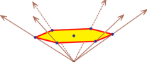
Figure 2. The hexagon and its lift.

In Exercise 3, you are asked to show that any finite set ${\mathcal{A}}\subset{\mathbb{Z}}^{1+n}$ lying on an affine hyperplane has the form ${\mathcal{B}}^{+}$ in appropriate coordinates for ${\mathbb{Z}}{\mathcal{A}}$. Exercise 4 gives another (equivalent) characterization of a set ${\mathcal{A}}$ lying on an affine hyperplane.

We turn to a geometric description of the generators of a homogeneous toric ideal $I_{\mathcal{A}}$. A sum $\sum_{a\in{\mathcal{A}}}a\lambda_{a}$ where $\sum_{a\in{\mathcal{A}}}\lambda_{a}=1$ and $0\leq\lambda_{a}$ is a convex combination of the points of ${\mathcal{A}}$. The convex hull of ${\mathcal{A}}\subset{\mathbb{Z}}^{n}$ is the set of all convex combinations of the points of ${\mathcal{A}}$,

$${\operatorname{\rm conv}({\mathcal{A}})}\ :=\ \Bigl{\{}\sum_{a\in{\mathcal{A}}}a\lambda_{a}\ \Bigl{|}\ \sum_{a\in{\mathcal{A}}}\lambda_{a}=1\mbox{ and }0\leq\lambda_{a}\mbox{ for all }a\in{\mathcal{A}}\Bigr{\}}\,.$$

This convex hull is a polytope with integer vertices (a lattice polytope), and its vertices are a subset of ${\mathcal{A}}$. Lattice polygons were depicted in Exercise 6 of Section 1 and in Figure 2. Below are a lattice simplex (${\mathcal{A}}$ corresponds to the matrix $\bigl{(}\mbox{\tiny$\begin{smallmatrix}0&1&0&0\\ 0&0&1&0\\ 0&0&0&1\end{smallmatrix}$}\bigr{)}$), a lattice cube (${\mathcal{A}}$ corresponds to the matrix $\bigl{(}\mbox{\tiny$\begin{smallmatrix}0&1&0&0&1&0&0&1\\ 0&0&1&0&1&0&1&1\\ 0&0&0&1&0&0&1&1\end{smallmatrix}$}\bigr{)}$), and a lattice octahedron (${\mathcal{A}}$ corresponds to the matrix $\bigl{(}\mbox{\tiny$\begin{smallmatrix}0&1&-1&0&0&0&0\\ 0&0&0&1&-1&0&0\\ 0&0&0&0&0&1&-1\end{smallmatrix}$}\bigr{)}$).

(2.3)                         

Let ${\mathcal{A}}\subset{\mathbb{Z}}^{1+n}$ lie on an affine hyperplane. Suppose that $u,v\in{\mathbb{N}}^{\mathcal{A}}$ are nonzero vectors with $u\neq v$ and ${\mathcal{A}}u={\mathcal{A}}v$ so that $z^{u}-z^{v}$ is a binomial in $I_{\mathcal{A}}$. By our assumption on ${\mathcal{A}}$, the toric ideal $I_{\mathcal{A}}$ is homogeneous, so that $\deg z^{u}=\deg z^{v}$. Let $d:=\sum_{a}u_{a}=\sum_{a}v_{a}$ be this degree. Writing ${\lambda_{a}}:=\frac{1}{d}u_{a}$ and ${\mu_{a}}:=\frac{1}{d}v_{a}$ for $a\in{\mathcal{A}}$, we have

$$\sum_{a\in{\mathcal{A}}}a\lambda_{a}\ =\ \sum_{a\in{\mathcal{A}}}a\mu_{a}\,.$$

As $\lambda_{a},\mu_{a}\geq 0$ are rational numbers and $\sum_{a}\lambda_{a}=\sum_{a}\mu_{a}=1$, this is a point in $\operatorname{\rm conv}({\mathcal{A}})$ having two distinct representations as a rational convex combination of the points of ${\mathcal{A}}$.

Suppose that ${\mathcal{A}}w=0$. Then $z^{w^{+}}-z^{w^{-}}$ is a generator for $I_{\mathcal{A}}$, by Corollary 1.4. Note that $\operatorname{\rm supp}(w^{+})$ is disjoint from $\operatorname{\rm supp}(w^{-})$. (Here, the support $\operatorname{\rm supp}(v)$ of a vector $v$ is the set of indices of nonzero coordinates.) Then the above construction (applied to $w^{+}$ and $w^{-}$) gives

$$\sum_{a\in\operatorname{\rm supp}(w^{+})}a\lambda_{a}\ =\ \sum_{a\in\operatorname{\rm supp}(w^{-})}a\mu_{a}\,,$$

which is a rational point common to the convex hulls of two disjoint subsets of ${\mathcal{A}}$.

Example 2.4.

Suppose that ${\mathcal{A}}$ is represented by the matrix $(\begin{smallmatrix}0&1&1&2&2\\ 1&0&2&0&1\end{smallmatrix})$. The point $(\frac{3}{2},\frac{1}{2})^{T}$ lies in the convex hull of two disjoint subsets of ${\mathcal{A}}$, $(\begin{smallmatrix}1&2\\ 0&1\end{smallmatrix})$ and $(\begin{smallmatrix}0&1&2\\ 1&2&0\end{smallmatrix})$, respectively.

These coincident convex combinations give the binomial $z_{(\mbox{\tiny$\begin{smallmatrix}1\\ 0\end{smallmatrix}$})}^{3}z_{(\mbox{\tiny$\begin{smallmatrix}2\\ 1\end{smallmatrix}$})}^{3}-z_{(\mbox{\tiny$\begin{smallmatrix}0\\ 1\end{smallmatrix}$})}z_{(\mbox{\tiny$\begin{smallmatrix}1\\ 2\end{smallmatrix}$})}z_{(\mbox{\tiny$\begin{smallmatrix}2\\ 0\end{smallmatrix}$})}^{4}$ in $I_{{\mathcal{A}}^{+}}$.

We summarize this discussion.

Proposition 2.5.

Suppose that ${\mathcal{A}}$ lies on an affine hyperplane. Homogeneous generators $z^{w^{+}}-z^{w^{-}}$ of $I_{\mathcal{A}}$ of Corollary 1.4 correspond to rational points of $\operatorname{\rm conv}({\mathcal{A}})$ lying in the intersection of convex hulls of two disjoint subsets of ${\mathcal{A}}$.

For a finite subset ${\mathcal{A}}\subset M\simeq{\mathbb{Z}}^{n}$, a cocharacter $w\in N$ (or any vector in ${N_{\mathbb{R}}}:=N\otimes_{\mathbb{Z}}{\mathbb{R}}$) gives a function on ${\mathcal{A}}$, where $a\mapsto w\cdot a$. Write $h_{\mathcal{A}}(w)$ for the maximum value this function takes on points of ${\mathcal{A}}$. The function $w\mapsto h_{\mathcal{A}}(w)$ is the support function of ${\mathcal{A}}$. The subset of ${\mathcal{A}}$ where the function $a\mapsto w\cdot a$ attains its maximum,

(2.4) $${{\mathcal{A}}_{w}}\ :=\ \{a\in{\mathcal{A}}\mid w\cdot a=h_{\mathcal{A}}(w)\}\,,$$

is the face of ${\mathcal{A}}$ exposed by $w$. When ${\mathcal{A}}$ is the set of column vectors of $\bigl{(}\mbox{\tiny$\begin{smallmatrix}0&1&0&0&1&0&0&1\\ 0&0&1&0&1&0&1&1\\ 0&0&0&1&0&0&1&1\end{smallmatrix}$}\bigr{)}$, which are the vertices of the lattice cube, the face exposed by the vector $(1,2,3)$ is the vertex $\bigl{(}\mbox{\tiny$\begin{smallmatrix}1\\ 1\\ 1\end{smallmatrix}$}\bigr{)}$, the face exposed by the vector $(1,-2,0)$ is the subset $\{\bigl{(}\mbox{\tiny$\begin{smallmatrix}1\\ 0\\ 1\end{smallmatrix}$}\bigr{)},\bigl{(}\mbox{\tiny$\begin{smallmatrix}1\\ 0\\ 0\end{smallmatrix}$}\bigr{)}\}$ that spans an edge of the cube, and the face exposed by the vector $(0,0,-1)$ is the subset $\{\bigl{(}\mbox{\tiny$\begin{smallmatrix}0\\ 0\\ 0\end{smallmatrix}$}\bigr{)},\bigl{(}\mbox{\tiny$\begin{smallmatrix}0\\ 1\\ 0\end{smallmatrix}$}\bigr{)},\bigl{(}\mbox{\tiny$\begin{smallmatrix}1\\ 0\\ 0\end{smallmatrix}$}\bigr{)},\bigl{(}\mbox{\tiny$\begin{smallmatrix}1\\ 1\\ 0\end{smallmatrix}$}\bigr{)}\}$, which spans the downward-pointing facet.

A face of ${\mathcal{A}}$ is any subset of this form. These same notions of support function $h_{P}(w)$, face $F$ of $P$, and face $P_{w}$ of $P$ exposed by $w$, also hold for any polytope $P$. Each face ${\mathcal{F}}$ of ${\mathcal{A}}$ is the intersection of ${\mathcal{A}}$ with a face $F$ of its convex hull $\operatorname{\rm conv}({\mathcal{A}})$, and $F=\operatorname{\rm conv}({\mathcal{F}})$. The inclusion ${\mathcal{F}}\subset{\mathcal{A}}$ of subsets induces an inclusion of projective spaces ${\mathbb{P}}^{\mathcal{F}}\subset{\mathbb{P}}^{\mathcal{A}}$, where ${\mathbb{P}}^{\mathcal{F}}$ is identified with the coordinate subspace $\{z\in{\mathbb{P}}^{\mathcal{A}}\mid z_{a}=0\mbox{ if }a\not\in{\mathcal{F}}\}$ of ${\mathbb{P}}^{\mathcal{A}}$. We state a relation between faces of ${\mathcal{A}}$ and toric subvarieties of $X_{\mathcal{A}}$ without proof.

Lemma 2.6.

Let $X_{\mathcal{A}}\subset{\mathbb{P}}^{\mathcal{A}}$ be the projective toric variety given by finite set ${\mathcal{A}}\subset{\mathbb{Z}}^{1+n}$ lying on an affine hyperplane. For any point $z\in X_{\mathcal{A}}$, its support $\operatorname{\rm supp}(z)=\{a\in{\mathcal{A}}\mid z_{a}\neq 0\}$ is a face of ${\mathcal{A}}$. For every face ${\mathcal{F}}$ of ${\mathcal{A}}$, the intersection $X_{\mathcal{A}}\cap{\mathbb{P}}^{\mathcal{F}}$ is naturally identified with $X_{\mathcal{F}}$.

There is much more relating the structure of the polytope $\operatorname{\rm conv}({\mathcal{A}})$ and the toric variety. We state another such result without proof. Consider the map ${\mu_{\mathcal{A}}}\colon{\mathbb{P}}^{\mathcal{A}}\to\operatorname{\rm conv}({\mathcal{A}})$ given by

$${\mathbb{P}}^{\mathcal{A}}\ \ni\ z=[z_{a}\mid a\in{\mathcal{A}}]\ \longmapsto\ \frac{\sum_{a\in{\mathcal{A}}}a|z_{a}|}{\sum_{a\in{\mathcal{A}}}|z_{a}|}\ \in\ \operatorname{\rm conv}({\mathcal{A}})\,.$$

Lemma 2.7.

The map $\mu_{\mathcal{A}}\colon X_{{\mathcal{A}}^{+}}\to\operatorname{\rm conv}({\mathcal{A}})$ is surjective. The inverse image of a face $F$ of $\operatorname{\rm conv}({\mathcal{A}})$ is $X_{\mathcal{F}}$, where ${\mathcal{F}}=F\cap{\mathcal{A}}$. The map $\mu_{\mathcal{A}}$ remains surjective when restricted to $X_{{\mathcal{A}}^{+}}({\mathbb{R}})=X_{{\mathcal{A}}^{+}}\cap{\mathbb{P}}^{\mathcal{A}}({\mathbb{R}})$, where ${\mathbb{P}}^{\mathcal{A}}({\mathbb{R}})={\mathbb{P}}({\mathbb{R}}^{\mathcal{A}})$, and also to

$$X_{{\mathcal{A}}^{+}}({\mathbb{R}}_{\geq})\ :=\ \{x=[x_{a}\mid a\in{\mathcal{A}}]\in X_{{\mathcal{A}}^{+}}\mid x_{a}\geq 0\mbox{ for all }a\in{\mathcal{A}}\}\,,$$

on which it is a homeomorphism. This map identifies $X_{{\mathcal{A}}^{+}}({\mathbb{R}})$ with $2^{n}$ copies of $\operatorname{\rm conv}({\mathcal{A}})$ glued along facets.

2.2. Kushnirenko’s Theorem

We turn to one of the most celebrated applications of toric varieties, understanding the number of solutions to a system of polynomial equations. A Laurent polynomial $f\in{\mathbb{C}}[x^{\pm}]$ is a finite linear combination of monomials. That is, there are coefficients $c_{a}\in{\mathbb{C}}$ for $a\in{\mathbb{Z}}^{n}$ such that

$$f\ =\ \sum_{a}c_{a}x^{a}\,,$$

with at most finitely many coefficients $c_{a}$ nonzero. The set ${\mathcal{A}}$ of indices of nonzero coefficients is called the support of $f$ and its convex hull $\operatorname{\rm conv}({\mathcal{A}})$ is the Newton polytope of $f$, which is a lattice polytope. We consider the number of solutions in $({\mathbb{C}}^{*})^{n}$ to a system

(2.5) $$f_{1}(x)\ =\ f_{2}(x)\ =\ \dotsb\ =\ f_{n}(x)\ =\ 0$$

of (Laurent) polynomial equations, where each polynomial has the same support ${\mathcal{A}}$. The coefficients of a polynomial identify ${\mathbb{C}}^{\mathcal{A}}$ with the set of polynomials whose support is a subset of ${\mathcal{A}}$, and $({\mathbb{C}}^{\mathcal{A}})^{n}$ is identified with set of polynomial systems (2.5) with support ${\mathcal{A}}$. Kushnirenko [12] proved the following count for the number of solutions to a system of polynomial equations (2.5) with support ${\mathcal{A}}$.

Theorem 2.8 (Kushnirenko).

A system (2.5) of $n$ polynomials in $n$ variables with support ${\mathcal{A}}$ has at most $n!\mbox{\rm Vol}(\operatorname{\rm conv}({\mathcal{A}}))$ isolated solutions in $({\mathbb{C}}^{*})^{n}$, counted with multiplicity. There is a dense open subset of $({\mathbb{C}}^{\mathcal{A}})^{n}$ consisting of systems with support ${\mathcal{A}}$ having exactly $n!\mbox{\rm Vol}(\operatorname{\rm conv}({\mathcal{A}}))$ solutions in $({\mathbb{C}}^{*})^{n}$, each isolated and occurring with multiplicity one.

Lemma 4.10 of Section 4 establishes the claim that there is an open set in $({\mathbb{C}}^{\mathcal{A}})^{n}$ of systems with support ${\mathcal{A}}$ all of which have the same number of isolated solutions and where each solution occurs with multiplicity one. Theorem 4.11 describes the discriminant conditions that imply all solutions are isolated. Namely, that for each $w\in{\mathbb{R}}^{n}$, the facial system

(2.6) $$f_{1,w}(x)\ =\ f_{2,w}(x)\ =\ \dotsb\ =\ f_{n,w}(x)\ =\ 0$$

has no solutions in $({\mathbb{C}}^{\times})^{n}$, where, for a Laurent polynomial $f$ with support ${\mathcal{A}}$, $f_{w}$ is the restriction of $f$ to the monomials in ${\mathcal{A}}_{w}$. This is also the initial form $\mbox{\rm in}_{w}f$ of $f$ with respect to the weighted partial term order $\prec_{w}$. This partial term order is defined in Exercise 12, where you are asked to prove the previous claim.

We use the projective toric variety $X_{{\mathcal{A}}^{+}}$ to prove Kushnirenko’s Theorem. The map $\varphi_{\mathcal{A}}$ parameterizes $X_{{\mathcal{A}}^{+}}$, and we first understand when this parametrization is injective. The affine span of a set ${\mathcal{A}}$ is

(2.7) $${\operatorname{\rm Aff}{\mathcal{A}}}\ :=\ \Bigl{\{}\sum_{a\in{\mathcal{A}}}a\lambda_{a}\mid\sum_{a\in{\mathcal{A}}}\lambda_{a}=1\Bigr{\}}\,.$$

This differs from the convex hull in that the coefficients $\lambda_{a}$ may be negative. When $\lambda_{a}\in{\mathbb{Z}}$, this is the integral affine span $\operatorname{\rm Aff}_{\mathbb{Z}}{\mathcal{A}}$. For any $a\in{\mathcal{A}}$, the affine span is the coset

(2.8) $$\operatorname{\rm Aff}{\mathcal{A}}\ =\ a\ +\ {\mathbb{R}}\{b-a\mid b\in{\mathcal{A}}\}\,,$$

and the same (replacing ${\mathbb{Z}}$ for ${\mathbb{R}}$) gives the integral affine span.

The map $\varphi_{\mathcal{A}}\colon({\mathbb{C}}^{*})^{n}\to{\mathbb{P}}^{\mathcal{A}}$ is the restriction of $\varphi_{{\mathcal{A}}^{+}}$ (2.2) to the subtorus $\{1\}\times({\mathbb{C}}^{*})^{n}$ of the torus ${\mathbb{C}}^{*}\times({\mathbb{C}}^{*})^{n}$ where $t=1$. In Exercise 6 you are asked to show that $\varphi_{\mathcal{A}}$ is injective if and only if $\operatorname{\rm Aff}_{\mathbb{Z}}{\mathcal{A}}={\mathbb{Z}}^{n}$. Notice that if $0\in{\mathcal{A}}$, then $\operatorname{\rm Aff}_{\mathbb{Z}}{\mathcal{A}}={\mathbb{Z}}{\mathcal{A}}$. Since multiplying a Laurent polynomial by a monomial $x^{a}$ does not change its set of zeros, it is no loss of generality to assume that $0\in{\mathcal{A}}$, in which case $\varphi_{\mathcal{A}}$ is injective if and only if ${\mathbb{Z}}{\mathcal{A}}={\mathbb{Z}}^{n}$. As $0\in{\mathcal{A}}$, one of the coordinates of $\varphi_{\mathcal{A}}$ is 1, so its image lies in a standard affine patch of ${\mathbb{P}}^{\mathcal{A}}$.

We relate the projective toric variety $X_{{\mathcal{A}}^{+}}$ to systems of polynomials with support ${\mathcal{A}}$. Given a (homogeneous) linear form $\Lambda$ on ${\mathbb{P}}^{\mathcal{A}}$,

$${\Lambda}\ =\ \sum_{a\in{\mathcal{A}}}c_{a}z_{a}\,,$$

its pullback $\varphi^{*}_{{\mathcal{A}}}(\Lambda)$ along $\varphi_{{\mathcal{A}}}$ is a polynomial with support ${\mathcal{A}}$,

$$\varphi^{*}_{{\mathcal{A}}}(\Lambda)\ =\ \sum_{a\in{\mathcal{A}}}c_{a}x^{a}\,.$$

Consequently, a system of $n$ polynomials (2.5) with support ${\mathcal{A}}$ is the pullback along $\varphi_{\mathcal{A}}$ of a system of $n$ linear forms on ${\mathbb{P}}^{\mathcal{A}}$. Note that a linear form $\Lambda$ on ${\mathbb{P}}^{\mathcal{A}}$ defines a hyperplane $H\subset{\mathbb{P}}^{\mathcal{A}}$ and $n$ general linear forms define a linear subspace $L$ of codimension $n$.

Lemma 2.9.

The solution set of a system of polynomials (2.5) with support ${\mathcal{A}}$ is the pullback $\varphi_{{\mathcal{A}}}^{-1}(L)=\varphi_{{\mathcal{A}}}^{-1}(L\cap\varphi_{\mathcal{A}}({{\mathbb{C}}^{*}}^{n}))$ of a linear section of $\varphi_{{\mathcal{A}}}({{\mathbb{C}}^{*}}^{n})$, where $L$ has codimension equal to the dimension of the linear span of the polynomials $f_{i}$.

Example 2.10.

Consider the polynomial system

(2.9) $${f}\ :=\ {x^{2}y+2xy^{2}-1+xy}\ =\ 0\quad\mbox{and}\quad{g}\ :=\ {x^{2}y-xy^{2}+2-xy}\ =\ 0\,.$$

These polynomials define two plane curves which have one real point of intersection at $(1.53277,-0.90655)$ and are displayed in Figure 3.

Figure 3. Curves of polynomial system (2.9).

The exponent vectors ${\mathcal{A}}$ are the columns of the matrix $(\begin{smallmatrix}2&1&0&1\\ 1&2&0&1\end{smallmatrix})$. The map $\varphi_{\mathcal{A}}$ is

$$(x,y)\ \longmapsto\ [x^{2}y\,:\ xy^{2}\,:\ 1\,:\ xy]\ \in{\mathbb{P}}^{\mathcal{A}}\simeq{\mathbb{P}}^{3}\,.$$

Its image consists of those points $[z_{(\mbox{\tiny$\begin{smallmatrix}2\\ 1\end{smallmatrix}$})}:z_{(\mbox{\tiny$\begin{smallmatrix}1\\ 2\end{smallmatrix}$})}:z_{(\mbox{\tiny$\begin{smallmatrix}0\\ 0\end{smallmatrix}$})}:z_{(\mbox{\tiny$\begin{smallmatrix}1\\ 1\end{smallmatrix}$})}]$ with $z_{(\mbox{\tiny$\begin{smallmatrix}2\\ 1\end{smallmatrix}$})}z_{(\mbox{\tiny$\begin{smallmatrix}1\\ 2\end{smallmatrix}$})}z_{(\mbox{\tiny$\begin{smallmatrix}0\\ 0\end{smallmatrix}$})}=z_{(\mbox{\tiny$\begin{smallmatrix}1\\ 1\end{smallmatrix}$})}^{3}\neq 0$, which is part of a cubic surface. The polynomial system (2.9) corresponds to the two linear forms

$$z_{(\mbox{\tiny$\begin{smallmatrix}2\\ 1\end{smallmatrix}$})}+2z_{(\mbox{\tiny$\begin{smallmatrix}1\\ 2\end{smallmatrix}$})}-z_{(\mbox{\tiny$\begin{smallmatrix}0\\ 0\end{smallmatrix}$})}+z_{(\mbox{\tiny$\begin{smallmatrix}1\\ 1\end{smallmatrix}$})}\ =\ z_{(\mbox{\tiny$\begin{smallmatrix}2\\ 1\end{smallmatrix}$})}-z_{(\mbox{\tiny$\begin{smallmatrix}1\\ 2\end{smallmatrix}$})}+2z_{(\mbox{\tiny$\begin{smallmatrix}0\\ 0\end{smallmatrix}$})}-z_{(\mbox{\tiny$\begin{smallmatrix}1\\ 1\end{smallmatrix}$})}\ =\ 0\,.$$

These define a line $\ell$ in ${\mathbb{P}}^{3}$. Figure 4 shows $\ell$ and (part of) the cubic surface. This is in the affine part of ${\mathbb{P}}^{\mathcal{A}}$ where $z_{(\mbox{\tiny$\begin{smallmatrix}1\\ 1\end{smallmatrix}$})}\neq 0$ near the origin. The best view is from the $+-+$-orthant.

Figure 4. Linear section of cubic surface.

From this, we see that there is one real solution to the system (2.9).

Lemma 2.9 gives an interpretation for the number $d({\mathcal{A}})$ of solutions to a general system (2.5) with support ${\mathcal{A}}$. The degree, $\deg(X)$, of a subvariety $X$ of ${\mathbb{P}}^{m}$ of dimension $n$ is the number of points in a linear section $L\cap X$ of $X$, where $L$ is a general linear subspace in ${\mathbb{P}}^{\mathcal{A}}$ of codimension $n$. Since a general linear subspace of codimension $n$ meets the toric variety $X_{{\mathcal{A}}^{+}}$ only at points in the image $\varphi_{\mathcal{A}}(({\mathbb{C}}^{*})^{n})$, and by Exercise 6, $\varphi_{\mathcal{A}}$ is injective if and only if $\operatorname{\rm Aff}_{\mathbb{Z}}{\mathcal{A}}={\mathbb{Z}}^{n}$, we deduce the following.

Lemma 2.11.

When the affine span of ${\mathcal{A}}$ is ${\mathbb{Z}}^{n}$, $d({\mathcal{A}})=\deg(X_{{\mathcal{A}}^{+}})$.

We prove Kushnirenko’s Theorem in the case when $\operatorname{\rm Aff}_{\mathbb{Z}}{\mathcal{A}}={\mathbb{Z}}^{n}$ by showing that

$$n!\cdot\mbox{\rm Vol}(\operatorname{\rm conv}({\mathcal{A}}))\ =\ \deg(X_{{\mathcal{A}}^{+}})\,$$

This proof is due to Khovanskii [11] and the presentation is adapted from Chapter 3 of [14], where the general case of $\operatorname{\rm Aff}_{\mathbb{Z}}{\mathcal{A}}\subsetneq{\mathbb{Z}}^{n}$ is deduced from the case when $\operatorname{\rm Aff}_{\mathbb{Z}}{\mathcal{A}}={\mathbb{Z}}^{n}$.

The homogeneous coordinate ring ${\mathbb{C}}[X]$ of a projective variety $X\subset{\mathbb{P}}^{\mathcal{A}}$ is the quotient of the homogeneous coordinate ring ${\mathbb{C}}[z_{a}\mid a\in{\mathcal{A}}]$ of ${\mathbb{P}}^{\mathcal{A}}$ by the ideal $I_{X}$ of homogeneous polynomials vanishing on $X$. These rings and ideals are graded by the total degree of the polynomials. Writing ${\mathbb{C}}_{d}[X]$ for the $d$th graded piece of ${\mathbb{C}}[X]$, the Hilbert function $\operatorname{\rm HF}_{X}(d)$ is the function $d\mapsto\dim_{\mathbb{C}}{\mathbb{C}}_{d}[X]$.

Hilbert proved that the Hilbert function for $d\gg 0$ is equal to a polynomial, which is now called the Hilbert polynomial $\operatorname{\rm HP}_{X}(d)$ of $X$. This encodes many numerical invariants of $X$. For example, the degree of the Hilbert polynomial is the dimension $n$ of $X$ and its leading coefficient is $\frac{1}{n!}\deg(X)$. For a discussion of Hilbert polynomials, see Section 9.3 of [4].

We determine the Hilbert polynomial of the toric variety $X_{{\mathcal{A}}^{+}}$. Its homogeneous coordinate ring is the coordinate ring of $X_{{\mathcal{A}}^{+}}\subset{\mathbb{C}}^{\mathcal{A}}$. By Corollary 1.3, this is ${\mathbb{C}}[{\mathbb{N}}{\mathcal{A}}^{+}]$. As the first coordinate $1$ of points of ${\mathcal{A}}^{+}$ corresponds to the homogenizing parameter $t$ in (2.2), ${\mathbb{C}}[{\mathbb{N}}{\mathcal{A}}^{+}]$ is graded by the first component of elements of ${\mathbb{N}}{\mathcal{A}}^{+}$. Thus ${\mathbb{C}}_{d}[{\mathbb{N}}{\mathcal{A}}^{+}]$ has a basis $\{(d,a)\in{\mathbb{N}}{\mathcal{A}}^{+}\}$. This is ${\mathbb{N}}{\mathcal{A}}^{+}\cap d\operatorname{\rm conv}({\mathcal{A}}^{+})$, which is equal to ${d{\mathcal{A}}^{+}}$, the set of $d$-fold sums of vectors in ${\mathcal{A}}^{+}$.

Example 2.12.

Consider this for the projectivization $X_{{\mathcal{A}}^{+}}$ of the cuspidal cubic of Example 1.1. Here, ${\mathcal{A}}=\{0,2,3\}$ and $\varphi_{\mathcal{A}}(s)=[1,s^{2},s^{3}]\in{\mathbb{P}}^{\mathcal{A}}$. Figure 5 shows its lift ${\mathcal{A}}^{+}=(\begin{smallmatrix}1&1&1\\ 0&2&3\end{smallmatrix})$ and the submonoid ${\mathbb{N}}{\mathcal{A}}^{+}$.

Figure 5. Monoid generated by the lift of $\{0,2,3\}$.

The open circles are points that do not lie in ${\mathbb{N}}{\mathcal{A}}^{+}$. The Hilbert function of $X_{{\mathcal{A}}^{+}}$ has values $(1,3,6,9,12,\dotsc)$, so its Hilbert polynomial is $3d$.

Projecting the set $d{\mathcal{A}}^{+}$ to the last $n$ coordinates is a bijection with the set $d{\mathcal{A}}$ of $d$-fold sums of vectors in ${\mathcal{A}}$. These arguments show that

$$\operatorname{\rm HF}_{X_{\mathcal{A}}}(d)\ =\ |d{\mathcal{A}}|\,.$$

Thus an upper bound on $\operatorname{\rm HF}_{X_{\mathcal{A}}}(d)$ is given by $|d\operatorname{\rm conv}({\mathcal{A}})\cap{\mathbb{Z}}^{n}|$, as $d{\mathcal{A}}\subset d\operatorname{\rm conv}({\mathcal{A}})\cap{\mathbb{Z}}^{n}$. Ehrhart [7] (see also [2]) showed that for an integer polytope $P$, the counting function

$${E_{P}}\ \colon\ {\mathbb{N}}\ni d\ \longmapsto\ |dP\cap{\mathbb{Z}}^{n}|$$

for the integer points contained in positive integer multiples of $P$ is a polynomial in $d$, now called the Ehrhart polynomial of $P$. The degree of $E_{P}$ is the dimension of the affine span of $P$. When $P$ has dimension $n$, its leading coefficient is the volume of $P$. For example, the Ehrhart polynomial of the interval $[0,3]=\operatorname{\rm conv}\{0,2,3\}$ of length 3 is $3d+1$.

Now suppose that $P=\operatorname{\rm conv}({\mathcal{A}})$, the convex hull of ${\mathcal{A}}$. Since $d{\mathcal{A}}\subset d\operatorname{\rm conv}({\mathcal{A}})\cap{\mathbb{Z}}^{n}$, we have the upper bound for $\operatorname{\rm HF}_{X_{\mathcal{A}}}(d)$,

(2.10) $$\operatorname{\rm HF}_{X_{\mathcal{A}}}(d)\ \leq\ E_{\operatorname{\rm conv}({\mathcal{A}})}(d)\,.$$

Note that we have this inequality for the cubic of Example 2.12.

A lower bound for $\operatorname{\rm HF}_{X_{\mathcal{A}}}(d)$ is best expressed in terms of an inclusion. Let ${S_{\mathcal{A}}}:={\mathbb{R}}_{\geq}{\mathcal{A}}^{+}\cap{\mathbb{Z}}^{1+n}$ be the monoid of all integer points that are in the nonnegative span of ${\mathcal{A}}^{+}$. The inequality (2.10) arises from the inclusion ${\mathbb{N}}{\mathcal{A}}^{+}\subset S_{\mathcal{A}}$ by considering points with first coordinate $d$. We will produce a vector $v\in{\mathbb{N}}{\mathcal{A}}^{+}$ and show that $v+S_{\mathcal{A}}\subset{\mathbb{N}}{\mathcal{A}}^{+}$, which we will use to show our lower bound.

Let ${{\mathcal{B}}}\subset S_{\mathcal{A}}$ be the set of points $b\in{\mathbb{Z}}^{n}$ which may be written as

$$b\ =\ \sum_{a\in{\mathcal{A}}}\lambda_{a}(1,a)\,,$$

where $\lambda_{a}$ is a rational number in $[0,1)$. For the set ${\mathcal{A}}=\{0,2,3\}$ of Example 2.12, ${\mathcal{B}}$ is origin, together with the four points in the interior of the hexagonal shaded region (a zonotope). These are the columns of the matrix $(\begin{smallmatrix}0&1&1&2&2\\ 0&1&2&3&4\end{smallmatrix})$.

For each $b\in{\mathcal{B}}$, fix an expression

(2.11) $$b\ =\ \sum_{a\in{\mathcal{A}}}\beta_{a}(b)(1,a)\qquad(\beta_{a}(b)\in{\mathbb{Z}})$$

as an integer linear combination of elements of ${\mathcal{A}}^{+}$. Let $-\nu$ with $\nu\geq 0$ be an integer lower bound for the coefficients $\beta_{a}(b)$ in these expressions for the finitely many elements $b\in{\mathcal{B}}$. For the set ${\mathcal{A}}=\{0,2,3\}$, we may take these expressions to be $(\begin{smallmatrix}1\\ 1\end{smallmatrix})=(\begin{smallmatrix}1\\ 0\end{smallmatrix})-(\begin{smallmatrix}1\\ 2\end{smallmatrix})+(\begin{smallmatrix}1\\ 3\end{smallmatrix})$, $(\begin{smallmatrix}1\\ 2\end{smallmatrix})=(\begin{smallmatrix}1\\ 2\end{smallmatrix})$, $(\begin{smallmatrix}2\\ 3\end{smallmatrix})=(\begin{smallmatrix}1\\ 0\end{smallmatrix})+(\begin{smallmatrix}1\\ 3\end{smallmatrix})$, and $(\begin{smallmatrix}2\\ 4\end{smallmatrix})=2(\begin{smallmatrix}1\\ 2\end{smallmatrix})$, so that $\nu=1$. Finally, define

$${v}\ :=\ \nu\cdot\sum_{a\in A}(1,a)\,.$$

Its first coordinate is $\nu|{\mathcal{A}}|$. For the set ${\mathcal{A}}=\{0,2,3\}$, this vector is $(\begin{smallmatrix}3\\ 5\end{smallmatrix})=(\begin{smallmatrix}1\\ 0\end{smallmatrix})+(\begin{smallmatrix}1\\ 2\end{smallmatrix})+(\begin{smallmatrix}1\\ 3\end{smallmatrix})$.

We claim that we have the inclusion of sets

(2.12) $$v+S_{\mathcal{A}}\ \subset\ {\mathbb{N}}{\mathcal{A}}^{+}\ \subset\ S_{\mathcal{A}}\,.$$

Comparing these sets at any level $d\geq\nu|{\mathcal{A}}|$ gives the inequality

$$E_{\operatorname{\rm conv}({\mathcal{A}})}(d-\nu|{\mathcal{A}}|)\ \leq\ \operatorname{\rm HF}_{X_{\mathcal{A}}}(d)\ \leq\ E_{\operatorname{\rm conv}({\mathcal{A}})}(d)\,,$$

Since both the lower bound and the upper bound are polynomials in $d$ of the same degree and leading term, we deduce that the Hilbert polynomial $\operatorname{\rm HP}_{X_{\mathcal{A}}}(d)$ has the same degree and leading term as the Ehrhart polynomial $E_{\operatorname{\rm conv}({\mathcal{A}})}$.

Thus the Hilbert polynomial has degree $n$ and its leading coefficient is the volume of $\operatorname{\rm conv}({\mathcal{A}})$. Since the degree of $X_{{\mathcal{A}}^{+}}$ is $n!$ times this leading coefficient, we conclude that the degree of $X_{{\mathcal{A}}^{+}}$ is

$$n!\;\mbox{\rm Vol}(\operatorname{\rm conv}({\mathcal{A}}))\,,$$

which proves Kushnirenko’s Theorem when $\operatorname{\rm Aff}_{\mathbb{Z}}{\mathcal{A}}={\mathbb{Z}}^{n}$, given the inclusions (2.12).

We establish the first inclusion in (2.12). (The second was already discussed.) Let $u\in v+S_{\mathcal{A}}$. Then $u-v\in S_{\mathcal{A}}$ and so it has an expression

$$u-v\ =\ \sum_{a\in{\mathcal{A}}}\alpha_{a}(1,a)\quad\mbox{ with }\quad\alpha_{a}\in{\mathbb{Q}}_{\geq}\,.$$

Writing each coefficient $\alpha_{a}$ in terms of its fractional and integral parts gives $\alpha_{a}=\lambda_{a}+\gamma_{a}$ where $\lambda_{a}\in[0,1)\cap{\mathbb{Q}}$ and $\gamma_{a}\in{\mathbb{N}}$. Then

$$u-v\ =\ \sum_{a\in{\mathcal{A}}}\lambda_{a}(1,a)\ +\ \sum_{a\in{\mathcal{A}}}\gamma_{a}(1,a)\ =\ b\ +\ c\,,$$

where $b\in{\mathcal{B}}$ and $c\in{\mathbb{N}}{\mathcal{A}}^{+}$. Using the fixed expression (2.11) for $b$, we have

$$w\ =\ v+\sum_{a}\beta_{a}(b)(1,a)\ +\ c\ =\ \sum_{s}(\beta_{a}(b)+\nu)(1,a)\ +\ c\,,$$

which lies in ${\mathbb{N}}{\mathcal{A}}^{+}$ as $-\nu\leq\beta_{a}$. This establishes the inclusion of sets (2.12) and completes the proof of Kushnirenko’s Theorem when $\operatorname{\rm Aff}_{\mathbb{Z}}{\mathcal{A}}={\mathbb{Z}}^{n}$.

The vector $v$ used to establish the inclusion (2.12) may be replaced by a more economical vector. For each $a\in A$, set ${\nu_{a}}:=\max\{0,-\beta_{a}(b)\mid b\in{\mathcal{B}}\}$. If we set ${v^{\prime}}:=\sum_{a\in{\mathcal{A}}}\nu_{a}(1,a)$, then the same argument shows that we still have an inclusion $v^{\prime}+S_{\mathcal{A}}\subset{\mathbb{N}}{\mathcal{A}}^{+}$. For ${\mathcal{A}}=\{0,2,3\}$ with ${\mathcal{A}}^{+}=(\begin{smallmatrix}1&1&1\\ 0&2&3\end{smallmatrix})$ the new vector $v^{\prime}$ is $(\begin{smallmatrix}1\\ 2\end{smallmatrix})$. Figure 6

Figure 6. Inclusions of cones for ${\mathcal{A}}=\{0,2,3\}$.

shows the monoid $S_{\mathcal{A}}$ (all the circles, filled and unfilled), the monoid ${\mathbb{N}}{\mathcal{A}}^{+}$ (the filled circles), the translate $(\begin{smallmatrix}1\\ 2\end{smallmatrix})+S_{\mathcal{A}}$ (larger shaded region), and finally the translate $(\begin{smallmatrix}3\\ 5\end{smallmatrix})+S_{\mathcal{A}}$ (smaller shaded region). Observe that $(\begin{smallmatrix}1\\ 2\end{smallmatrix})$ is the shortest vector such that the translate $(\begin{smallmatrix}1\\ 2\end{smallmatrix})+S_{\mathcal{A}}$ lies in ${\mathbb{N}}{\mathcal{A}}^{+}$.

The expression $n!\;\mbox{\rm Vol}(\operatorname{\rm conv}({\mathcal{A}}))$ in Kushnirenko’s Theorem is often called the normalized volume of $\operatorname{\rm conv}({\mathcal{A}})$.

Exercises

1. Verify that the subgroup ${\mathbb{Z}}{\mathcal{A}}$ for the set ${\mathcal{A}}=(\begin{smallmatrix}3&2&1&0\\ 0&1&2&3\end{smallmatrix})$ of Example 2.2 is a full rank (rank 2) subgroup of index 3 in ${\mathbb{Z}}^{2}$. You may find the map ${\mathbb{Z}}^{2}\to{\mathbb{Z}}$ given by $(p,q)\mapsto p+q$ useful; consider its kernel, image, and cokernel, and the restrictions to ${\mathbb{Z}}{\mathcal{A}}$.

2. Let ${\mathcal{A}}\subset{\mathbb{Z}}^{n}$ be a finite set of points. Show that its lift ${\mathcal{A}}^{+}\subset{\mathbb{Z}}^{1+n}$ spans ${\mathbb{Z}}^{1+n}$ if and only if the set of differences $\{a-b\mid\forall a,b\in{\mathcal{A}}\}$ spans ${\mathbb{Z}}^{n}$.

3. Prove that if a finite set ${\mathcal{A}}\subset{\mathbb{Z}}^{n}$ lies on an affine hyperplane and $\operatorname{\rm rank}({\mathbb{Z}}{\mathcal{A}})=1+m$, then there is a basis for ${\mathbb{Z}}{\mathcal{A}}$ identifying it with ${\mathbb{Z}}^{1+m}$ and a subset ${\mathcal{B}}\subset{\mathbb{Z}}^{m}$ such that ${\mathcal{A}}={\mathcal{B}}^{+}$.

4. Suppose that ${\mathcal{A}}\subset{\mathbb{Z}}^{n}$ is represented by an integer matrix, $A$. Show that ${\mathcal{A}}$ lies on an affine hyperplane if and only if the row space of $A$ in ${\mathbb{R}}^{\mathcal{A}}$ has a vector with every coordinate 1.

5. Prove the equivalence of the two definitions, (2.7) and (2.8), of affine span.

6. Let ${\mathcal{A}}\subset{\mathbb{Z}}^{n}$ be finite. Show that the map $\varphi_{\mathcal{A}}\colon({\mathbb{C}}^{*})^{n}\to{\mathbb{P}}^{\mathcal{A}}$ is injective if and only if the integral affine span ${\mathbb{Z}}{\mathcal{A}}$ of ${\mathcal{A}}$ is ${\mathbb{Z}}^{n}$.

7. Give a spanning set of degree two generators for $I_{\mathcal{A}}$, where ${\mathcal{A}}$ is the lifted hexagon of Figure 2. Interpret each generator as a point common to the convex hulls of two disjoint subsets of ${\mathcal{A}}$.

8. Repeat Exercise 7 for (a) the lift of the cube and (b) the lift of the octahedron.

               

9. Do the homogeneous version of Exercise 6 from Section 1. For a polygon $P$, let ${\mathcal{A}}_{P}:=P\cap{\mathbb{Z}}^{2}$ be the set of integer points in $P$, and ${\mathcal{A}}^{+}_{P}$ the lift of these points to ${\mathbb{Z}}^{3}$. For each polygon $P$ below, identify homogeneous binomials that generate the homogeneous toric ideal $I_{{\mathcal{A}}^{+}_{P}}$. For each generator, give the coincident convex combination of Proposition 2.5, and the point of $P$ to which it corresponds.

                                   

   Are homogeneous toric ideals always generated by quadratic binomials?

10. Show that the Euclidean volume of the simplex $\operatorname{\rm conv}\{0,e_{1},\dotsc,e_{n}\}$ is $\frac{1}{n!}$, where $e_{i}$ is the standard coordinate unit vector in ${\mathbb{R}}^{n}$. Harder: Prove that this is the minimum volume of any lattice simplex, and that all others have volume an integer multiple of $\frac{1}{n!}$.

11. Determine the volume of the Newton polytope of the Laurent polynomial

    $$1+x+2y+3z-4xyz+5x^{2}y+7yz^{2}+11x^{2}z^{2}+13xy^{3}z+17y^{3}z^{2}-8x^{2}y^{2}z^{2}\,.$$

    Hint: use a computer algebra system to determine the number of solutions to a general sparse system with this support and apply Kushnirenko’s Theorem. Challenge: Can you use this method to prove the volume is what you computed?

12. Let $f\in{\mathbb{C}}[x^{\pm}]$ and let ${\mathcal{A}}:=\operatorname{\rm supp}(f)$. For any $w\in{\mathbb{R}}^{n}$, we have a partial term order on ${\mathbb{C}}[x^{\pm}]$ given by

    $$x^{a}\ {\prec_{w}}\ x^{b}\qquad\text{if}\qquad w\cdot a\ <\ w\cdot b\,.$$

    Show that $\operatorname{\rm supp}(\mbox{\rm in}_{w}f)={\mathcal{A}}_{w}$, where ${\mathcal{A}}_{w}$ is defined in (2.4).

13. For a challenging exercise, provide a proof of Lemma 2.6.

14. For an even more challenging exercise, provide a proof of Lemma 2.7.

3. Toric Varieties From Fans

Affine toric varieties $X_{\mathcal{A}}$ are given by a finite collection ${\mathcal{A}}$ of integer vectors. The ideal of an affine toric variety is generated by binomials coming from elements of the integer kernel of a linear map determined by the set ${\mathcal{A}}$. When the set ${\mathcal{A}}$ lies on an affine hyperplane, the toric variety $X_{\mathcal{A}}$ is homogeneous and gives a projective toric variety with structure corresponding to the polytope $\operatorname{\rm conv}({\mathcal{A}})$. We give an abstract (not embedded) construction of a toric variety obtained by gluing affine toric varieties, where the affine varieties and the gluing are encoded in an object from geometric combinatorics called a rational fan.

Example 3.1.

The projective line ${\mathbb{P}}^{1}$ is the projective toric variety given by columns ${\mathcal{A}}$ of the matrix $(\begin{smallmatrix}1&0\\ 0&1\end{smallmatrix})$. The corresponding integer polytope is the convex hull of the two points of ${\mathcal{A}}$, which in an appropriate coordinate system is just the interval $[0,1]$.

In its homogeneous coordinates $[x,y]$, ${\mathbb{P}}^{1}$ has two standard affine patches ${{\mathbb{C}}_{0}}:=[x,1]$ for $x\in{\mathbb{C}}$ and ${{\mathbb{C}}_{\infty}}:=[1,y]$ for $y\in{\mathbb{C}}$. Their intersection ${\mathbb{C}}_{0}\cap{\mathbb{C}}_{\infty}$ may be identified with ${\mathbb{C}}^{*}$; it is the points of either patch where the parameter ($x$ for ${\mathbb{C}}_{0}$ and $y$ for ${\mathbb{C}}_{\infty}$) does not vanish. The point $[x,1]\in{\mathbb{C}}_{0}^{*}$ is identified with the point $[1,x^{-1}]\in{\mathbb{C}}_{\infty}^{*}$. Consequently, ${\mathbb{P}}^{1}$ is the union of two copies of ${\mathbb{C}}$, ${\mathbb{C}}_{0}\sqcup{\mathbb{C}}_{\infty}$, glued along this common set.

We organize this using subalgebras of ${\mathbb{C}}[x,x^{-1}]$. First, ${\mathbb{C}}_{0}=\operatorname{\rm spec}{\mathbb{C}}[x]$, which is identified with $\mbox{\rm Hom}_{m}({\mathbb{N}},{\mathbb{C}})$, where a point $[x,1]\in{\mathbb{C}}_{0}$ is the monoid homomorphism $f_{x}$ that sends the generator $1\in{\mathbb{N}}$ to $x\in{\mathbb{C}}$ and $f_{x}(0)=11$ as it is a homomorphism of monoids. Similarly, ${\mathbb{C}}_{\infty}=\operatorname{\rm spec}{\mathbb{C}}[x^{-1}]=\mbox{\rm Hom}_{m}(-{\mathbb{N}},{\mathbb{C}})$. Here, a point $[1,y]$ is the monoid homomorphism $g_{y}$ that sends the generator $-1$ to $y\in{\mathbb{C}}$. Also, ${\mathbb{C}}^{*}=\operatorname{\rm spec}{\mathbb{C}}[x,x^{-1}]$, which is $\mbox{\rm Hom}_{m}({\mathbb{Z}},{\mathbb{C}})$, where a point $z\in{\mathbb{C}}^{*}$ is the monoid homomorphism $h_{z}$ that sends $0\mapsto 1$ and $1\mapsto z$. The restriction of $h_{z}$ to ${\mathbb{N}}$ gives the map $f_{z}$ and its restriction to $-{\mathbb{N}}$ is the map $g_{z^{-1}}$.

3.1. Cones and Fans

We develop more geometric combinatorics needed for the remaining material on toric varieties, in the context of objects in ${\mathbb{R}}^{n}$. For additional reference, we recommend the books of Ewald [9] and Ziegler [15].

Let ${\mathcal{A}}\subset{\mathbb{R}}^{n}$ be a finite set. As explained in Section 2, its convex hull

$${\operatorname{\rm conv}({\mathcal{A}})}\ :=\ \Bigl{\{}\sum_{a\in{\mathcal{A}}}a\lambda_{a}\mid\sum_{a\in{\mathcal{A}}}\lambda_{a}=1\mbox{ and }0\leq\lambda_{a}\mbox{ for all }a\in{\mathcal{A}}\Bigr{\}}$$

is a polytope, $P$. This polytope is a closed and bounded set, so for $w\in{\mathbb{R}}^{n}$, the linear function on ${\mathbb{R}}^{n}$ given by $x\mapsto w\cdot x$ is bounded on $P$, and thus has a maximum value, $h_{P}(w)$, on $P$. This function $w\mapsto h_{P}(w)$ is the support function of $P$. The subset ${P_{w}}:=\{x\in P\mid w\cdot x=h_{P}(w)\}$ of $P$ where this maximum is attained is the face of $P$ exposed by $w$, and is again a polytope, typically of smaller dimension. It is the convex hull of ${\mathcal{A}}_{w}$, which is the set of points $a\in{\mathcal{A}}$ where $w\cdot a=h_{P}(w)$. (These notions were treated in Subsection 2.1.) The dimension of a polytope is the dimension of its affine span. A face $F$ of $P$ of dimension zero is a point and it is called a vertex of $P$. A face of dimension one is a line segment, and it is called an edge. A facet of $P$ is a face $F$ with codimension one, $\dim F=\dim P{-}1$.

Example 3.2.

A useful construction of one polytope from another is a pyramid. Suppose that $P$ is a polytope of dimension $n{-}1$, which we assume lies on a hyperplane $H$ defined by $w\cdot x=b$ in ${\mathbb{R}}^{n}$ for some $0\neq w\in{\mathbb{R}}^{n}$ ($H=\{x\in{\mathbb{R}}^{n}\mid w\cdot x=b\}$). For any point $o\in{\mathbb{R}}^{n}\smallsetminus H$, the pyramid with base $P$ and apex $o\in{\mathbb{R}}^{n}$ is the convex hull of the polytope $P$ and the point $o$. This pyramid has height $h:=\frac{1}{\|w\|}|b-w\cdot o|=|w\cdot(o-x)|/\|w\|$ for any $x\in H$, and its volume is $\frac{1}{n}h\mbox{\rm Vol}_{n-1}(P)$.

By the definition of the support function $h_{P}(w)$ of $P$, for any $w\in{\mathbb{R}}^{n}$, we have

$$P\ \subset\ \{x\in{\mathbb{R}}^{n}\mid w\cdot x\leq h_{P}(w)\}\,.$$

This set is a half space and its boundary $\{x\mid w\cdot x=h_{P}(w)\}$ is a supporting hyperplane of $P$. Note that $P_{w}$ is the intersection of $P$ with the supporting hyperplane corresponding to $w$. As a closed, convex body, $P$ is the intersection of all half-spaces that contain it,

(3.1) $$P\ =\ \bigcap_{w\in{\mathbb{R}}^{n}}\{x\in{\mathbb{R}}^{n}\mid w\cdot x\leq h_{P}(w)\}\,.$$

For example, the lattice octahedron (2.3) $\{(x,y,z)\in{\mathbb{R}}^{3}\mid|x|+|y|+|z|\leq 1\}$ is the intersection of the eight half spaces, $\{(x,y,z)\in{\mathbb{R}}^{3}\mid\pm x\pm y\pm z\leq 1\}$, one for each choice of the three signs $\pm$. The lattice pentagon is the intersection of five half spaces,

$$\raisebox{-21.0pt}{\includegraphics{figures/LatticePentagon.eps}}\ =\ \raisebox{-21.0pt}{\includegraphics{figures/LatticePentagon1.eps}}\ \bigcap\ \raisebox{-21.0pt}{\includegraphics{figures/LatticePentagon2.eps}}\ \bigcap\ \raisebox{-21.0pt}{\includegraphics{figures/LatticePentagon3.eps}}\ \bigcap\ \raisebox{-21.0pt}{\includegraphics{figures/LatticePentagon4.eps}}\ \bigcap\ \raisebox{-21.0pt}{\includegraphics{figures/LatticePentagon5.eps}}\ .$$

In these examples, the polytope $P$ is the intersection of finitely many half spaces, one for each facet of $P$. This is true for all polytopes.

Proposition 3.3.

A polytope $P$ is the intersection of finitely many half spaces, one for each facet of $P$.

A polyhedron is the intersection of finitely many half spaces, and a bounded polyhedron is a polytope. Here are four unbounded polyhedra in ${\mathbb{R}}$, ${\mathbb{R}}^{2}$, ${\mathbb{R}}^{2}$, and ${\mathbb{R}}^{3}$, respectively.

                        

A polyhedron $P$ has a support function $h_{P}(w)$ that takes values in ${\mathbb{R}}\cup\{\infty\}$. When $P$ is unbounded in the direction of $w$, then $h_{P}(w)=\infty$. With this definition, the description (3.1) holds for $P$.

A (convex) cone is a polyhedron for which each supporting hyperplane contains the origin, and is therefore a linear subspace. Equivalently, a cone $\sigma$ is a polyhedron whose support function only takes values 0 and $\infty$. The half spaces that define a cone all have the form

$$\{x\in{\mathbb{R}}^{n}\mid w\cdot x\leq 0\}\,.$$

Such a half space forms an additive monoid under addition and its boundary hyperplane is a linear space consisting of the invertible elements in this monoid.

Consequently, a cone $\sigma$ is a monoid under addition and the intersection of its boundary hyperplanes is a linear subspace $\ell$ of ${\mathbb{R}}^{n}$, called the lineality space of $\sigma$. The lineality space is the set of invertible elements in $\sigma$. When the lineality space is the origin, the cone is pointed (also called strictly convex or strongly convex). A face $\tau$ of a cone $\sigma$ is again a cone and the lineality space of $\sigma$ is its minimal face. Figure 7 shows four cones, two in ${\mathbb{R}}^{2}$ and two in ${\mathbb{R}}^{3}$.

Figure 7. Four cones.

The first and the third are pointed, while the second and fourth have a one-dimensional lineality space. The second is a half space.

The origin is the minimal face of a pointed cone $\sigma$. The rays of a pointed cone $\sigma$ are its one-dimensional faces. Each ray $\rho$ has the form ${\mathbb{R}}_{\geq}x$ for any nonzero element $x$ of $\rho$. While a polytope is the convex hull of its vertices, a pointed cone is the sum of its rays. For example, the third cone in Figure 7 is ${\mathbb{R}}_{\geq}\bigl{(}\mbox{\tiny$\begin{smallmatrix}0\\ 1\\ 2\end{smallmatrix}$}\bigr{)}+{\mathbb{R}}_{\geq}\bigl{(}\mbox{\tiny$\begin{smallmatrix}0\\ -1\\ 2\end{smallmatrix}$}\bigr{)}+{\mathbb{R}}_{\geq}\bigl{(}\mbox{\tiny$\begin{smallmatrix}1\\ 0\\ 2\end{smallmatrix}$}\bigr{)}+{\mathbb{R}}_{\geq}\bigl{(}\mbox{\tiny$\begin{smallmatrix}-1\\ 0\\ 2\end{smallmatrix}$}\bigr{)}$. More generally, any cone is a sum of rays. The fourth cone in Figure 7 is ${\mathbb{R}}_{\geq}\bigl{(}\mbox{\tiny$\begin{smallmatrix}0\\ 1\\ 2\end{smallmatrix}$}\bigr{)}+{\mathbb{R}}_{\geq}\bigl{(}\mbox{\tiny$\begin{smallmatrix}0\\ -1\\ 2\end{smallmatrix}$}\bigr{)}+{\mathbb{R}}_{\geq}\bigl{(}\mbox{\tiny$\begin{smallmatrix}1\\ 0\\ 0\end{smallmatrix}$}\bigr{)}+{\mathbb{R}}_{\geq}\bigl{(}\mbox{\tiny$\begin{smallmatrix}-1\\ 0\\ 0\end{smallmatrix}$}\bigr{)}$.

Another important object is a polyhedral complex. This is a collection ${\mathcal{P}}$ of polyhedra in ${\mathbb{R}}^{d}$ such that every face of every polyhedron in ${\mathcal{P}}$ is another polyhedron in ${\mathcal{P}}$ and the intersection of any two polyhedra $P,P^{\prime}$ in ${\mathcal{P}}$ is a common face of each. For example, of the four collections of vertices, line segments, and polyhedra below, the first three are polyhedral complexes, while the last is not; the large triangle does not meet either of the smaller triangles in one of its faces.

                  

A polytope together with all of its faces forms a polyhedral complex. The boundary of a polytope (all of its proper faces) forms a polyhedral complex. For a less simple example, suppose that $o\in P$ is any point of a polytope $P$. For every face $F$ of $P$ that does not contain $o$ we may consider the pyramid with base $F$ and apex $o$. This collection of pyramids, their bases, and the apex $o$ forms a polyhedral subdivision of $P$.

The support of a polyhedral complex ${\mathcal{P}}$ is the union of the polyhedra in ${\mathcal{P}}$. When the support of a polyhedral complex is a polyhedron $P$, the complex is a subdivision of $P$. When the support is a polytope $P$, we have the following formula for the volume of $P$,

$$\mbox{\rm Vol}_{n}(P)\ =\ \sum_{Q\in{\mathcal{P}}}\mbox{\rm Vol}_{n}(Q)\,.$$

When every polytope in a polyhedral complex ${\mathcal{P}}$ is a simplex, we say that ${\mathcal{P}}$ is a triangulation of its support. Of the four polyhedral subdivisions below, the last two are triangulations.

                  

Our last object in this tour of geometric combinatorics is a fan, which is a polyhedral complex, all of whose polyhedra are cones. If the support of a fan is the ambient space, then the fan is said to be complete. Figure 8 shows some fans in ${\mathbb{R}}^{2}$ and ${\mathbb{R}}^{3}$.

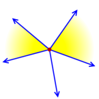
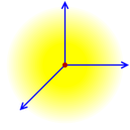
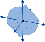
Figure 8. Three fans.

The second is complete, and the third is complete, if we include the eight implied open cones.

Given a polytope $P$ in ${\mathbb{R}}^{n}$, define an equivalence relation on the dual ${\mathbb{R}}^{n}$ by $v\sim w$ if and only if $P_{v}=P_{w}$, so that $v$ and $w$ expose the same face of $P$. The closure of each equivalence class is a cone in ${\mathbb{R}}^{n}$, and these cones together form the (outer) normal fan to the polytope $P$, which is a complete fan. The rays of the normal fan expose facets of $P$.

Example 3.4.

The third fan in Figure 8 is the outer normal fan to the lattice cube (2.3). Indeed, the standard unit vectors $\bigl{(}\mbox{\tiny$\begin{smallmatrix}1\\ 0\\ 0\end{smallmatrix}$}\bigr{)}$, $\bigl{(}\mbox{\tiny$\begin{smallmatrix}0\\ 1\\ 0\end{smallmatrix}$}\bigr{)}$, and $\bigl{(}\mbox{\tiny$\begin{smallmatrix}0\\ 0\\ 1\end{smallmatrix}$}\bigr{)}$, together with their negatives, $\bigl{(}\mbox{\tiny$\begin{smallmatrix}-1\\ 0\\ 0\end{smallmatrix}$}\bigr{)}$, $\bigl{(}\mbox{\tiny$\begin{smallmatrix}0\\ -1\\ 0\end{smallmatrix}$}\bigr{)}$, and $\bigl{(}\mbox{\tiny$\begin{smallmatrix}0\\ 0\\ -1\end{smallmatrix}$}\bigr{)}$, expose the six facets of the cube. An edge between two facets exposed by vectors $v$ and $w$ is exposed by any vector $\lambda v+\mu w$ where $\lambda,\mu>0$, and all vectors in the interior of each orthant expose the same vertex.

For more examples, we display a regular heptagon and a lattice hexagon, together with their normal fans.

                        

Here are two views of the same polytope in ${\mathbb{R}}^{3}$, together with its normal fan having the same orientation.

                        

The magenta ray in the normal fan is normal to the magenta facet, the green ray exposes the green edge, and the cyan ray exposes the cyan edge.

3.2. Toric Varieties From Fans

We give a construction of a toric variety by gluing affine toric varieties together along common open subsets. This is the original construction/definition of a toric variety from [6]. As in Sections 1 and 2, we work with the torus $({\mathbb{C}}^{*})^{n}$, its group $N=\mbox{\rm Hom}({\mathbb{C}}^{*},({\mathbb{C}}^{*})^{n})\simeq{\mathbb{Z}}^{n}$ of cocharacters, and its group $M=\mbox{\rm Hom}(({\mathbb{C}}^{*})^{n},{\mathbb{C}}^{*})\simeq{\mathbb{Z}}^{n}$ of characters. Let ${N_{\mathbb{R}}}:={\mathbb{R}}\otimes_{\mathbb{Z}}N\simeq{\mathbb{R}}^{n}$ be the real vector space spanned by the cocharacters and ${M_{\mathbb{R}}}:={\mathbb{R}}\otimes_{\mathbb{Z}}M\simeq{\mathbb{R}}^{n}$ be the real vector space spanned by the characters. Note that $N\subset N_{\mathbb{R}}$ and $M\subset M_{\mathbb{R}}$ in the same way as ${\mathbb{Z}}^{n}\subset{\mathbb{R}}^{n}$. We write $\langle\bullet,\bullet\rangle\colon N_{\mathbb{R}}\times M_{\mathbb{R}}\to{\mathbb{R}}$ for the pairing between $N_{\mathbb{R}}$ and $M_{\mathbb{R}}$, extending that between $N$ and $M$.

A (rational) fan $\Sigma\subset N_{\mathbb{R}}$ is a fan in $N_{\mathbb{R}}$ in which every cone is defined by inequalities coming from elements $a$ of $M$. The half spaces defining the cones all have the form

$$\{w\in N_{\mathbb{R}}\mid\langle w,a\rangle\geq 0\}\qquad\mbox{ for some }\quad a\in M\,.$$

The linear span of a cone $\sigma$ in a rational fan $\Sigma$ is a rational linear space in that it is spanned by its intersection with $N$. The notions of rational fan and rational linear subspace also make sense in $M_{\mathbb{R}}$. We will assume that all cones in $\Sigma$ are pointed, as this simplifies the exposition. In general, all cones in a rational fan have the same lineality space, $L_{\mathbb{R}}$, which contains a full rank sublattice $L=N\cap L_{\mathbb{R}}$. Replacing $N$ by $N/L$, $M$ by $L^{\perp}$, and every cone $\sigma$ of $\Sigma$ by its image in $N_{\mathbb{R}}/L_{\mathbb{R}}$, we obtain a rational fan $\Sigma/L_{\mathbb{R}}$ that is pointed. The price we pay for this is that the torus for the resulting toric varieties is identified with its dense orbit, which leads to a loss of flexibility in our notion of toric variety: E.g. the closure of a torus orbit in such a toric variety is a subvariety that is a toric variety—but for a different torus.

Given a rational cone $\sigma\subset N_{\mathbb{R}}$, its dual cone is

$${\sigma^{\vee}}\ :=\ \{x\in M_{\mathbb{R}}\,\mid\,\langle w,x\rangle\geq 0\mbox{ for }w\in\sigma\}\,.$$

This rational cone has full dimension in $M_{\mathbb{R}}$. Its lineality space is $\sigma^{\perp}$, the annihilator of $\sigma$, which has dimension $n{-}\dim\sigma$. This is the set of $x\in M_{\mathbb{R}}$ such that $\langle w,x\rangle=0$ for all $w\in\sigma$.

Example 3.5.

The cone ${\mathbb{R}}_{\geq}(\mbox{\tiny$\begin{smallmatrix}1\\ 0\end{smallmatrix}$})+{\mathbb{R}}_{\geq}(\mbox{\tiny$\begin{smallmatrix}0\\ 1\end{smallmatrix}$})$ (the first quadrant in ${\mathbb{R}}^{2}$) has dual cone ${\mathbb{R}}_{\geq}(\mbox{\tiny$\begin{smallmatrix}1\\ 0\end{smallmatrix}$})+{\mathbb{R}}_{\geq}(\mbox{\tiny$\begin{smallmatrix}0\\ 1\end{smallmatrix}$})$, the first quadrant in the dual ${\mathbb{R}}^{2}$. More interesting is the cone $\sigma={\mathbb{R}}_{\geq}(\mbox{\tiny$\begin{smallmatrix}1\\ 2\end{smallmatrix}$})+{\mathbb{R}}_{\geq}(\mbox{\tiny$\begin{smallmatrix}2\\ 1\end{smallmatrix}$})$, whose dual cone is $\sigma^{\vee}={\mathbb{R}}_{\geq}(\mbox{\tiny$\begin{smallmatrix}2\\ -1\end{smallmatrix}$})+{\mathbb{R}}_{\geq}(\mbox{\tiny$\begin{smallmatrix}-1\\ 2\end{smallmatrix}$})$. We display all three cones below.

(3.2)         

We give an example in ${\mathbb{R}}^{3}$. The two-dimensional cone $\sigma={\mathbb{R}}_{\geq}\bigl{(}\mbox{\tiny$\begin{smallmatrix}1\\ 0\\ 0\end{smallmatrix}$}\bigr{)}+{\mathbb{R}}_{\geq}\bigl{(}\mbox{\tiny$\begin{smallmatrix}0\\ 1\\ 0\end{smallmatrix}$}\bigr{)}$ has dual cone $\sigma^{\vee}={\mathbb{R}}_{\geq}\bigl{(}\mbox{\tiny$\begin{smallmatrix}1\\ 0\\ 0\end{smallmatrix}$}\bigr{)}+{\mathbb{R}}_{\geq}\bigl{(}\mbox{\tiny$\begin{smallmatrix}0\\ 1\\ 0\end{smallmatrix}$}\bigr{)}+{\mathbb{R}}\bigl{(}\mbox{\tiny$\begin{smallmatrix}0\\ 0\\ 1\end{smallmatrix}$}\bigr{)}$, whose lineality space is the vertical axis.

    

Given a pointed rational cone $\sigma\subset N_{\mathbb{R}}$, set

$${S_{\sigma}}\ :=\ \sigma^{\vee}\cap M\ =\ \{a\in M\,\mid\,\langle w,a\rangle\geq 0\mbox{ for }w\in\sigma\}\,,$$

which is a submonoid of $M$. Its group of invertible elements is the free abelian group $\sigma^{\perp}\cap M$ which has rank $n-\dim\sigma$, the dimension of the lineality space $\sigma^{\perp}$ of $\sigma^{\vee}$. Finally, let ${V_{\sigma}}:=\mbox{\rm Hom}_{m}(S_{\sigma},{\mathbb{C}})$, the set of monoid homomorphisms from $S_{\sigma}$ to ${\mathbb{C}}$. As we saw in Section 1, this is equal to the spectrum of the monoid algebra ${\mathbb{C}}[S_{\sigma}]$ and so $V_{\sigma}$ is an affine toric variety. (This requires a theorem of Hilbert that such a monoid is finitely generated.) However, it is not naturally embedded in an affine space ${\mathbb{C}}^{\mathcal{A}}$. For this, we need to choose a set ${\mathcal{A}}\subset S_{\sigma}$ that generates $S_{\sigma}$ as a monoid, so that $S_{\sigma}={\mathbb{N}}{\mathcal{A}}$. This is this is equivalent to the surjectivity of the map ${\mathbb{N}}^{\mathcal{A}}\rightarrow S_{\sigma}$ given by $(n_{a}\mid a\in{\mathcal{A}})\mapsto\sum_{a}an_{a}$.

Example 3.6.

For the cone $\sigma={\mathbb{R}}_{\geq}(\mbox{\tiny$\begin{smallmatrix}1\\ 2\end{smallmatrix}$})+{\mathbb{R}}_{\geq}(\mbox{\tiny$\begin{smallmatrix}2\\ 1\end{smallmatrix}$})$, a generating set for $S_{\sigma}$ is ${\mathcal{A}}=(\mbox{\tiny$\begin{smallmatrix}2&1&0&-1\\ -1&0&1&2\end{smallmatrix}$})$, which is highlighted in (3.2). The map

$$\mbox{\rm Hom}_{m}(S_{\sigma},{\mathbb{C}})\ \ni\ f\ \longmapsto\ \bigl{(}f(\mbox{\tiny$\begin{smallmatrix}2\\ -1\end{smallmatrix}$}),f(\mbox{\tiny$\begin{smallmatrix}1\\ 0\end{smallmatrix}$}),f(\mbox{\tiny$\begin{smallmatrix}0\\ 1\end{smallmatrix}$}),f(\mbox{\tiny$\begin{smallmatrix}-1\\ 2\end{smallmatrix}$})\bigr{)}\ \in\ {\mathbb{C}}^{\mathcal{A}}$$

is an embedding of $V_{\sigma}$ into ${\mathbb{C}}^{\mathcal{A}}$. The image satisfies the equations

$$z_{(\mbox{\tiny$\begin{smallmatrix}2\\ -1\end{smallmatrix}$})}z_{(\mbox{\tiny$\begin{smallmatrix}0\\ 1\end{smallmatrix}$})}-z_{(\mbox{\tiny$\begin{smallmatrix}1\\ 0\end{smallmatrix}$})}^{2}\,,\ \ z_{(\mbox{\tiny$\begin{smallmatrix}2\\ -1\end{smallmatrix}$})}z_{(\mbox{\tiny$\begin{smallmatrix}-1\\ 2\end{smallmatrix}$})}-z_{(\mbox{\tiny$\begin{smallmatrix}1\\ 0\end{smallmatrix}$})}z_{(\mbox{\tiny$\begin{smallmatrix}0\\ 1\end{smallmatrix}$})}\,,\ \mbox{ and }\ z_{(\mbox{\tiny$\begin{smallmatrix}1\\ 0\end{smallmatrix}$})}z_{(\mbox{\tiny$\begin{smallmatrix}-1\\ 2\end{smallmatrix}$})}-z_{(\mbox{\tiny$\begin{smallmatrix}0\\ 1\end{smallmatrix}$})}^{2}\,,$$

which are given by the relations in $S_{\sigma}$ satisfied by elements of ${\mathcal{A}}$. These are the same equations as (2.1), and so this affine toric variety is the affine cone over the rational normal curve.

Suppose that $\tau$ is a face of a rational cone $\sigma\subset N_{\mathbb{R}}$. Then $\sigma^{\vee}\subset\tau^{\vee}$, as $\tau^{\vee}$ involves fewer inequalities. This gives an inclusion $S_{\sigma}\subset S_{\tau}$ of monoids, and that in turn gives an inclusion of affine toric varieties associated to these cones,

$$V_{\tau}\ =\ \mbox{\rm Hom}_{m}(S_{\tau},{\mathbb{C}})\ \subset\ \mbox{\rm Hom}_{m}(S_{\sigma},{\mathbb{C}})\ =\ V_{\sigma}\,.$$

Here, the inclusion is given by restricting a monoid homomorphism $g\colon S_{\tau}\to{\mathbb{C}}$ to the submonoid $S_{\sigma}$.

Definition 3.7.

Let $\Sigma\subset N_{\mathbb{R}}$ be a rational fan. The toric variety $X_{\Sigma}$ associated to $\Sigma$ is obtained from the collection $\{V_{\sigma}\mid\sigma\in\Sigma\}$ of affine toric varieties associated to cones in the fan $\Sigma$ by gluing along the natural inclusions $V_{\tau}\subset V_{\sigma}$ whenever $\tau,\sigma$ are cones in $\Sigma$ with $\tau$ a face of $\sigma$. As the minimal cone in $\Sigma$ is the origin ${\mathbf{0}}$ and ${\mathbf{0}}^{\perp}=M_{\mathbb{R}}$ so that $S_{{\mathbf{0}}}=M$. Thus $V_{\mathbf{0}}$ is the torus $\mbox{\rm Hom}_{m}(M,{\mathbb{C}})=\mbox{\rm Hom}_{g}(M,{\mathbb{C}}^{*})$. This lies in every affine toric patch $V_{\sigma}$ and the gluing is torus-equivariant. This shows that the toric variety $X_{\sigma}$ has an action of this torus.

Example 3.8.

Example 3.1 constructs the projective line ${\mathbb{P}}^{1}$ from the fan $\Sigma\subset{\mathbb{R}}$ whose cones are $\sigma={\mathbb{R}}_{\geq}$, the nonnegative real numbers, $\rho={\mathbb{R}}_{\leq}$, the nonpositive real numbers, and $\tau=\{0\}$, the origin.

Then $V_{\sigma}=\mbox{\rm Hom}_{m}({\mathbb{N}},{\mathbb{C}})$, $V_{\rho}=\mbox{\rm Hom}_{m}(-{\mathbb{N}},{\mathbb{C}})$, and $V_{\tau}=\mbox{\rm Hom}_{m}({\mathbb{Z}},{\mathbb{C}})$, which are the sets ${\mathbb{C}}_{0}$, ${\mathbb{C}}_{\infty}$, and ${\mathbb{C}}^{*}$ of Example 3.1, and the gluing is the same as in Example 3.1.

We give a detailed construction of a less trivial toric variety $X_{\Sigma}$ in Section 3.3.

We connect abstract toric varieties to the projective toric varieties of Section 2. For this, let $P\subset M_{\mathbb{R}}$ be a polytope with vertices in $M$ and set ${\mathcal{A}}:=P\cap M$. Write $X_{P}$ for the projective toric variety $X_{{\mathcal{A}}^{+}}$. Let ${\Sigma_{P}}\subset N_{\mathbb{R}}$ be the outer normal fan of $P$. Each cone $\sigma\in\Sigma_{P}$ corresponds to a unique face $P_{\sigma}$ of $P$. (Recall that each cone $\sigma\in\Sigma_{P}$ is the closure of the set of points of $N_{\mathbb{R}}$ that expose a given face of $P$.) More specifically, let $\sigma^{\circ}$ be the relative interior of $\sigma$, the set-theoretic difference of $\sigma$ with the union of its proper faces. Then $P_{\sigma}$ is the face of $P$ exposed by any point $w\in\sigma^{\circ}$. Also, the linear span of differences $b-a$ of points $a,b\in P_{\sigma}$ is the lineality space of $\sigma^{\vee}$.

For a cone $\sigma\in\Sigma_{P}$, we define a map $\phi_{\sigma}\colon V_{\sigma}\to{\mathbb{P}}^{\mathcal{A}}$ whose image lies in the projective toric variety $X_{P}$. Choose any point $b\in P_{\sigma}\cap M$. By the definition of $P_{\sigma}$, if $w\in\sigma$ and $a\in{\mathcal{A}}(=P\cap M)$, then $\langle w,b\rangle\geq\langle w,a\rangle$, so that $\langle w,b-a\rangle\geq 0$. Since this inequality holds for all $w\in\sigma$, we have that $b-a\in\sigma^{\vee}\cap M=S_{\sigma}$. For an element $f\in V_{\sigma}=\mbox{\rm Hom}_{m}(S_{\sigma},{\mathbb{C}})$, define ${\varphi_{b,\sigma}(f)}\in{\mathbb{P}}^{\mathcal{A}}$ to be the point $[f(b-a)\mid a\in{\mathcal{A}}]$. We note that the sign here, $b-a$ for $a\in{\mathcal{A}}$, is to conform with our use of the outer normal fan. For the inner normal fan, use $a-b$ for $a\in{\mathcal{A}}$.

Lemma 3.9.

For any two elements $b,b^{\prime}\in P_{\sigma}\cap M$ and $f\in V_{\sigma}$, we have that $\varphi_{b,\sigma}(f)=\varphi_{b^{\prime},\sigma}(f)$ as points in ${\mathbb{P}}^{\mathcal{A}}$. For any $f\in V_{\sigma}$, $\varphi_{b,\sigma}(f)\in X_{P}$. For any point $x\in X_{P}$ with $x_{c}\neq 0$ for $c\in P_{\sigma}\cap M$, there is a point $f\in V_{\sigma}$ with $x=\varphi_{b,\sigma}(f)$.

Proof.

For $b,b^{\prime}\in P_{\sigma}\cap M$, $b-b^{\prime}\in\sigma^{\perp}$ so that if $f\in V_{\sigma}$, then $f(b-b^{\prime})$ is a nonzero scalar. For any $a\in{\mathcal{A}}$, we have

$$f(b^{\prime}-a)\ =\ f(b^{\prime}-b+b-a)\ =\ f(b^{\prime}-b)\cdot f(b-a)\,,$$

as $f\in\mbox{\rm Hom}_{m}(S_{\sigma},{\mathbb{C}})$. Thus as points of ${\mathbb{C}}^{\mathcal{A}}$, $\varphi_{b^{\prime},\sigma}(f)=f(b^{\prime}-b)\varphi_{b,\sigma}(f)$, so they give the same point in ${\mathbb{P}}^{\mathcal{A}}$.

To see that $\varphi_{b,\sigma}(f)\in X_{P}=X_{{\mathcal{A}}^{+}}$, we show that $\varphi_{b,\sigma}(f)\in{\mathcal{V}}(I_{{\mathcal{A}}^{+}})$. By Theorem 1.2, it suffices to check that each binomial $z^{u}-z^{v}$ in $I_{{\mathcal{A}}^{+}}$ vanishes at $\varphi_{b,\sigma}(f)$. Suppose that $u,v\in{\mathbb{N}}^{\mathcal{A}}$ satisfies ${\mathcal{A}}^{+}u={\mathcal{A}}^{+}v$. Then ${\mathcal{A}}u={\mathcal{A}}v$ and $|u|=|v|$. We compute

$$\qquad\bigl{(}\varphi_{b,\sigma}(f)\bigr{)}^{u}\ =\ f\Bigl{(}\sum_{a\in{\mathcal{A}}}u_{a}(b-a)\Bigr{)}\ =\ f(|u|b-{\mathcal{A}}u)\\ =\ f(|v|b-{\mathcal{A}}v)\ =\ f\Bigl{(}\sum_{a\in{\mathcal{A}}}v_{a}(b-a)\Bigr{)}\ =\ \bigl{(}\varphi_{b,\sigma}(f)\bigr{)}^{v}\,,\qquad$$

and so $z^{u}-z^{v}$ vanishes at $\varphi_{b,\sigma}(f)$. Thus $\varphi_{b,\sigma}(f)\in{\mathcal{V}}(I_{{\mathcal{A}}^{+}})$. But this equals $X_{{\mathcal{A}}^{+}}$ as $I_{{\mathcal{A}}^{+}}$ is prime and hence radical, by Theorem 1.2.

Finally, suppose that $x=[x_{a}\mid a\in{\mathcal{A}}]\in X_{{\mathcal{A}}^{+}}$ is a point with $x_{c}\neq 0$ for some $c\in P_{\sigma}\cap M$. Choose any $b\in P_{\sigma}\cap M$ and define the monoid homomorphism $f\colon{\mathbb{N}}\{b-a\mid a\in{\mathcal{A}}\}\to{\mathbb{C}}$ by $f(b-a)=x_{a}x_{b}^{-1}$, and extend linearly. This is well-defined as $x\in X_{{\mathcal{A}}^{+}}$ and so $x^{u}=x^{v}$ and whenever ${\mathcal{A}}^{+}u={\mathcal{A}}^{+}v$. If $S_{\sigma}={\mathbb{N}}\{b-a\mid a\in{\mathcal{A}}\}$, this completes the proof. Otherwise, as $S_{\sigma}=M\cap{\mathbb{Q}}\{b-a\mid a\in{\mathcal{A}}\}$ and ${\mathbb{C}}$ is algebraically closed, we may extend $f$ to a monoid homomorphism of $S_{\sigma}$.

Thus we obtain a well-defined map ${\varphi_{\sigma}}\colon V_{\sigma}\to X_{P}\subset{\mathbb{P}}^{\mathcal{A}}$ whose image is the set of points of $X_{P}$ whose coordinates indexed by elements of $P_{\sigma}\cap M$ are nonzero.

Lemma 3.10.

Let $\sigma,\tau\in\Sigma$ be cones with $\tau\subset\sigma$. For any element $f\in V_{\tau}$, we have $\varphi_{\tau}(f)=\varphi_{\sigma}(f)$, where we apply $\varphi_{\sigma}$ to the image of $f$ under the natural inclusion $V_{\tau}\subset V_{\sigma}$.

Proof.

This is tautological. If $f\in V_{\tau}$, then its image in $V_{\sigma}$ is obtained by restricting $f$ from $S_{\tau}$ to the points of $S_{\sigma}$. Choosing $b\in P_{\tau}\cap M\subset P_{\sigma}\cap M$, we have that $\{b-a\mid a\in{\mathcal{A}}\}\subset S_{\sigma}\subset S_{\tau}$, so that $\varphi_{b,\tau}(f)=\varphi_{b,\sigma}(f)$, which completes the proof.

By Lemma 3.10, the map from the disjoint union of the $V_{\sigma}$ for $\sigma\in\Sigma$ to $X_{P}$ given by the collection of maps $\{\varphi_{\sigma}\mid\sigma\in\Sigma\}$ agrees on the inclusions $V_{\tau}\subset V_{\sigma}$ given by inclusions $\tau\subset\sigma$ of cones in $\Sigma$. Thus it induces a (surjective) map $\varphi_{P}\colon X_{\Sigma}\to X_{P}$. This map is in fact an isomorphism of algebraic varieties.

Remark 3.11.

A map similar to the map $\varphi_{P}\colon X_{\Sigma}\to X_{P}$ may also be defined for any set ${\mathcal{A}}\subset P\cap M$ such that $\operatorname{\rm conv}({\mathcal{A}})=P$. Its image will be the projective toric variety $X_{{\mathcal{A}}^{+}}$.

3.3. The Double Pillow

We illustrate the construction of toric varieties for the normal fan $\Sigma\subset{\mathbb{R}}^{2}$ of the diamond, , which is the convex hull of the column vectors of the matrix $(\begin{smallmatrix}0&-1&0&1&0\\ -1&0&0&0&1\end{smallmatrix})$. We display this lattice polygon and its normal fan $\Sigma$.

(3.3)             

The fan $\Sigma$ has four rays ${\mathbb{R}}_{\geq}(\begin{smallmatrix}\pm 1\\ \pm 1\end{smallmatrix})$ one for each of four choices of signs, and four two-dimensional cones spanned by adjacent rays.

Each two-dimensional cone $\sigma$ is self-dual and all are isomorphic. Thus $X_{\Sigma}$ is obtained by gluing together four isomorphic affine toric varieties $V_{\sigma}$, as $\sigma$ ranges over the two-dimensional cones in $\Sigma$. A complete picture of the gluing involves the affine varieties $V_{\tau}$, where $\tau$ a ray of $\Sigma$. We next describe these two toric varieties $V_{\sigma}$ and $V_{\tau}$, for $\sigma$ a two-dimensional cone of $\Sigma$ and $\tau$ a ray of $\Sigma$.

Let $\sigma$ be the shaded cone in (3.3). Since $\sigma=\sigma^{\vee}$, we see that $\sigma^{\vee}\cap\mathbb{Z}^{2}$ is minimally generated by the column vectors ${\mathcal{A}}$ of the matrix $(\begin{smallmatrix}1&1&1\\ -1&1&0\end{smallmatrix})$ highlighted in (3.3) and so $V_{\sigma}$ is isomorphic to the affine toric variety $X_{\mathcal{A}}$, which is the closure in ${\mathbb{C}}^{3}$ of the image of the map

$$\varphi\ \colon\ (s,t)\ \longmapsto\ (st^{-1},st,s)\,,$$

and is defined by the equation $z_{(\mbox{\tiny$\begin{smallmatrix}1\\ -1\end{smallmatrix}$})}z_{(\mbox{\tiny$\begin{smallmatrix}1\\ 1\end{smallmatrix}$})}=z_{(\mbox{\tiny$\begin{smallmatrix}1\\ 0\end{smallmatrix}$})}^{2}$. This is a cone in ${\mathbb{C}}^{3}$. We display its real points (a right circular cone) in ${\mathbb{R}}^{3}$ below at left.

(3.4)     

Let $\tau$ be the ray generated by $(\mbox{\tiny$\begin{smallmatrix}1\\ 1\end{smallmatrix}$})$, which is a face of $\sigma$. Then $\tau^{\vee}$ is the half-space $\{(u,v)\in{\mathbb{R}}^{2}\mid u+v\geq 0\}$, which is the union of both two-dimensional cones in $\Sigma$ containing $\tau$. Since $\tau^{\vee}\cap\mathbb{Z}^{2}$ has generators the column vectors ${\mathcal{B}}$ of the matrix $(\mbox{\tiny$\begin{smallmatrix}1&-1&1\\ -1&1&0\end{smallmatrix}$})$, $V_{\tau}$ is isomorphic to the affine toric variety $X_{\mathcal{B}}$, which is the closure in ${\mathbb{C}}^{3}$ of the image of the map

$$\varphi\ \colon\ (s,t)\ \longmapsto\ (st^{-1},s^{-1}t,s)\,,$$

and has equation $z_{(\mbox{\tiny$\begin{smallmatrix}1\\ -1\end{smallmatrix}$})}z_{(\mbox{\tiny$\begin{smallmatrix}-1\\ 1\end{smallmatrix}$})}=1$. This is the cylinder with base the hyperbola $z_{(\mbox{\tiny$\begin{smallmatrix}1\\ -1\end{smallmatrix}$})}z_{(\mbox{\tiny$\begin{smallmatrix}-1\\ 1\end{smallmatrix}$})}=1$ in the $z_{(\mbox{\tiny$\begin{smallmatrix}1\\ -1\end{smallmatrix}$})},z_{(\mbox{\tiny$\begin{smallmatrix}-1\\ 1\end{smallmatrix}$})}$-plane, which is shown in (3.4) (in ${\mathbb{R}}^{3}$) at right.

We describe the gluing. We have that $V_{\tau}\subset V_{\sigma}$ and they both contain the torus $({\mathbb{C}}^{*})^{2}$. In each, this common torus is its intersection with the complement of the coordinate planes in the given embedding, and the boundary of the torus is its intersection with the coordinate planes. The boundary of $({\mathbb{C}}^{*})^{2}$ in the cylinder $V_{\tau}$ is the curve $z_{(\mbox{\tiny$\begin{smallmatrix}1\\ 0\end{smallmatrix}$})}=0$ and $z_{(\mbox{\tiny$\begin{smallmatrix}1\\ -1\end{smallmatrix}$})}z_{(\mbox{\tiny$\begin{smallmatrix}-1\\ 1\end{smallmatrix}$})}=1$, which is displayed in (3.4) on the picture of $V_{\tau}$. Also, $t\neq 0$ on this cylinder. The boundary of $({\mathbb{C}}^{*})^{2}$ in the cone is the union of the $z_{(\mbox{\tiny$\begin{smallmatrix}1\\ -1\end{smallmatrix}$})}$- and $z_{(\mbox{\tiny$\begin{smallmatrix}1\\ 1\end{smallmatrix}$})}$-axes. Since $t=z_{(\mbox{\tiny$\begin{smallmatrix}1\\ 1\end{smallmatrix}$})}/z_{(\mbox{\tiny$\begin{smallmatrix}1\\ 0\end{smallmatrix}$})}$ on the cone, the locus where $t=0$ is the $z_{(\mbox{\tiny$\begin{smallmatrix}1\\ 1\end{smallmatrix}$})}$-axis. Thus $V_{\tau}$ is naturally identified with the complement of the $z_{(\mbox{\tiny$\begin{smallmatrix}1\\ 1\end{smallmatrix}$})}$-axis in $V_{\sigma}$ while the curve $z_{(\mbox{\tiny$\begin{smallmatrix}1\\ 0\end{smallmatrix}$})}=0$ and $z_{(\mbox{\tiny$\begin{smallmatrix}1\\ -1\end{smallmatrix}$})}z_{(\mbox{\tiny$\begin{smallmatrix}-1\\ 1\end{smallmatrix}$})}=1$ in $V_{\tau}$ is identified with the $z_{(\mbox{\tiny$\begin{smallmatrix}1\\ -1\end{smallmatrix}$})}$-axis in $V_{\sigma}$.

If $\tau^{\prime}$ is the other ray of $\sigma$, then $V_{\tau^{\prime}}$ ($\simeq V_{\tau}$) is identified with the complement of the $z_{(\mbox{\tiny$\begin{smallmatrix}1\\ -1\end{smallmatrix}$})}$-axis in $V_{\sigma}$. A convincing understanding of this gluing procedure may be obtained by considering an image of the real points of the toric variety $X_{\includegraphics[height=6.0pt]{figures/Diamond.eps}}$ in a projection to ${\mathbb{P}}^{3}$. (Recall that $X_{\Sigma}$ has a map to the projective toric variety $X_{\includegraphics[height=6.0pt]{figures/Diamond.eps}}\subset{\mathbb{P}}^{\mathcal{A}}={\mathbb{P}}^{4}$ which is an isomorphism.) The map ${\mathbb{P}}^{\mathcal{A}}\to{\mathbb{P}}^{3}$ is given by the points $[1:\pm 1:0:0]$ and $[1:0:\pm 1:0]$ associated to the vertices $(\pm 1,0)$ and $(0,\pm 1)$ of , and the vertical point at infinity $[0:0:0:1]$ associated to its center. (Here, the plane at infinity is $[0:x:y:z]$.) The image of the toric variety $X_{\includegraphics[height=6.0pt]{figures/Diamond.eps}}$ under this projection map ${\mathbb{P}}^{\mathcal{A}}\to{\mathbb{P}}^{3}$ is a rational surface in ${\mathbb{P}}^{3}$. An affine part of the real points of this surface is shown in Figure 9.

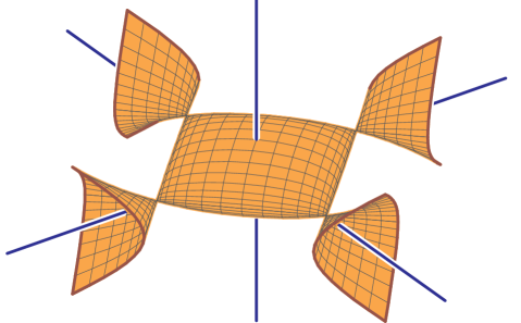
Figure 9. The double pillow.

In the coordinates $[w:x:y:z]$ for ${\mathbb{P}}^{3}$ this surface has the implicit equation

$$(x^{2}-y^{2})^{2}-2x^{2}w^{2}-2y^{2}w^{2}-16z^{2}w^{2}+w^{4}\ =\ 0\,.$$

and its dense torus has parametrization

$$[w:x:y:z]\ =\ [{\textstyle s+t+\frac{1}{s}+\frac{1}{t}\,:\ s-\frac{1}{s}\,:\ t-\frac{1}{t}\,:\ 1}]\,.$$

It has curves of self-intersection along the lines $x=\pm y$ in the plane at infinity ($w=0$). As the self-intersection is at infinity, this affine surface is a good illustration of the real points of the toric variety $X_{\includegraphics[height=6.0pt]{figures/Diamond.eps}}$, and so we refer to this picture to describe $X_{\includegraphics[height=6.0pt]{figures/Diamond.eps}}$.

This surface contains four lines $x\pm y=\pm 1$ and their complement is the dense torus in $X_{\includegraphics[height=6.0pt]{figures/Diamond.eps}}$. The complement of any three lines is the piece $V_{\tau}$ corresponding to a ray $\tau$. Each of the four singular points is a singular point of one cone $V_{\sigma}$, which is obtained by removing the two lines not meeting that singular point. Finally, the action of the group $\{(\pm 1,\pm 1)\}\subset({\mathbb{C}}^{*})^{2}$ on the real points $X_{\includegraphics[height=6.0pt]{figures/Diamond.eps}}({\mathbb{R}})$ may also be seen from this picture. Each singular point is fixed by this group. The element $(-1,-1)$ sends $z\mapsto-z$, interchanging the top and bottom halves of each piece, while the elements $(1,-1)$ and $(-1,1)$ interchange the central ‘pillow’ with the rest of $X_{\includegraphics[height=6.0pt]{figures/Diamond.eps}}({\mathbb{R}})$. In this way, we see that $X_{\includegraphics[height=6.0pt]{figures/Diamond.eps}}({\mathbb{R}})$ is a ‘double pillow’.

The nonnegative part $X_{\includegraphics[height=6.0pt]{figures/Diamond.eps}}({\mathbb{R}}_{\geq})$ of $X_{\includegraphics[height=6.0pt]{figures/Diamond.eps}}({\mathbb{R}})$ is also seen in Figure 9. The upper part of the middle pillow is the part of $X_{\includegraphics[height=6.0pt]{figures/Diamond.eps}}({\mathbb{R}})$ parameterized by ${\mathbb{R}}_{>}^{2}$, and so its closure is just a square, but with singular corners obtained by cutting a cone into two pieces along a plane of symmetry. This is $X_{\includegraphics[height=6.0pt]{figures/Diamond.eps}}({\mathbb{R}}_{\geq})$. In fact, the orthogonal projection to the $x,y$-plane identifies $X_{\includegraphics[height=6.0pt]{figures/Diamond.eps}}({\mathbb{R}}_{\geq})$ with the polygon . This is also a consequence of Lemma 2.7. The composition of the projection ${\mathbb{P}}^{\mathcal{A}}\to{\mathbb{P}}^{3}\to{\mathbb{P}}^{2}$, where the last is the orthogonal projection to the $x,y$-plane, is the projection map $\mu_{{\mathcal{A}}}$, at least on $X_{\includegraphics[height=6.0pt]{figures/Diamond.eps}}({\mathbb{R}}_{\geq})$. From the symmetry of this surface, we see that $X_{\includegraphics[height=6.0pt]{figures/Diamond.eps}}({\mathbb{R}})$ is obtained by gluing four copies of the polygon together along their edges to form two pillows attached at their corners. (The four ‘antennae’ are actually the truncated corners of the second pillow—projective geometry can play tricks on our affine intuition.)

Exercises

1. Show that the lattice octahedron (2.3) is the intersection of the eight half spaces, $\{(x,y,z)\in{\mathbb{R}}^{3}\mid\pm x\pm y\pm z\leq 1\}$, one for each choice of the three signs $\pm$.

2. Let ${\mathcal{A}}\subset{\mathbb{R}}^{n}$ be a finite set, and let $P=\operatorname{\rm conv}({\mathcal{A}})$ be its convex hull, a polytope. For $w\in{\mathbb{R}}^{n}$, recall that

   $${\mathcal{A}}_{w}\ =\ \{a\in{\mathcal{A}}\ |\ w\cdot a=h_{p}(w)\}\,.$$

   Let $P_{w}$ be the face of $P$ exposed by $w$. Show that

   $${\mathcal{A}}_{w}\ =\ {\mathcal{A}}\cap P_{w},.$$

3. Using the notation from the previous exercise, prove that $P_{w}=\operatorname{\rm conv}({\mathcal{A}}_{w})$.

4. Prove that a vertex (face of dimension zero) in a polyhedron $P$ is extreme in that it does not lie in the convex hull of other points of $P$. Deduce that a polytope is the convex hull of its vertices.

5. Show that every face of a cone is a cone, and that the minimal face is its lineality space.

6. Let $P\subset{\mathbb{R}}^{n}$ be a polytope. Show that for $v,w\in{\mathbb{R}}^{n}$, the relation

   $$v\ \sim\ w\ \Longleftrightarrow\ P_{v}=P_{w}$$

   is an equivalence relation. Show that the closure of an equivalence class is a cone, and if $P$ is in integer polytope, the cone is rational. (Hint: express an equivalence class in terms of the vertices of $P$.)

7. Determine the cones of the normal fan to the lattice cube, which you may take to be the convex hull of the vectors $\bigl{(}\mbox{\tiny$\begin{smallmatrix}\pm 1\\ \pm 1\\ \pm 1\end{smallmatrix}$}\bigr{)}$, for all eight choices of $\pm$.

8. Prove that the linear span of a cone $\sigma$ in a rational fan $\Sigma\subset{\mathbb{N}}_{\mathbb{R}}$ is spanned by its intersection with $N$.

9. The final paragraph in the proof of Lemma 3.9 is a bit dense. Fill in the details.

10. For each rational fan in ${\mathbb{R}}^{2}$ below, carry out the construction of the toric variety associated to the fan.

             

    Do you recognize either of these varieties?

4. Bernstein’s Theorem and Mixed Volumes

Bernstein [3] gave a formula for the number of solutions to a system of polynomials where different polynomials may have different supports, generalizing Kushnirenko’s Theorem. Bernstein’s formula is in terms of Minkowski’s mixed volume. We first review mixed volume, and then give a proof of Bernstein’s theorem, adapted from his paper, but using some elementary notions from tropical geometry. The discussion of mixed volumes is based on the pages 116–118 in [9].

4.1. Mixed Volumes

Recall that for a polytope $P\subset{\mathbb{R}}^{n}$, $\mbox{\rm Vol}(P)$ is its volume with respect to the standard Euclidean metric on ${\mathbb{R}}^{n}$. Write $\mbox{\rm Vol}_{n}(P)$ if we need to emphasize the ambient space of $P$. In particular, if $\dim P<n$, then $\mbox{\rm Vol}_{n}(P)=0$. If $\dim P=m$, then $\mbox{\rm Vol}_{m}(P)$ is taken to be its volume in its $m$-dimensional affine span. (This is used in the proof of Theorem 4.3.)

We consider two constructions involving polytopes. Let $P,Q\subset{\mathbb{R}}^{n}$ be polytopes and $\lambda\geq 0$ a real number. Then we may scale $P$ to obtain another polytope,

$${\lambda P}\ :=\ \{\lambda x\mid x\in P\}\,.$$

The Minkowski sum of $P$ and $Q$ is

$${P+Q}\ :=\ \{x+y\mid x\in P,y\in Q\}\,.$$

Note that $P+P=2P$.

Example 4.1.

Suppose that ${\mathcal{A}}$ is represented by the matrix $(\begin{smallmatrix}0&1&1&2&2\\ 1&0&2&0&1\end{smallmatrix})$ and ${\mathcal{B}}$ is represented by the matrix $(\begin{smallmatrix}0&1&1&2\\ 0&1&2&1\end{smallmatrix})$, and set $P:=\operatorname{\rm conv}({\mathcal{A}})$ and $Q:=\operatorname{\rm conv}({\mathcal{B}})$. Then $P+Q=\operatorname{\rm conv}({\mathcal{A}}+{\mathcal{B}})=\operatorname{\rm conv}({\mathcal{C}})$, where ${\mathcal{C}}$ is represented by the matrix $(\begin{smallmatrix}0&1&1&2&2&4&4\\ 1&0&3&0&4&1&2\end{smallmatrix})$. We display these polytopes and their Minkowski sum in Figure 10.

$$P\ =\ \raisebox{-20.0pt}{\includegraphics{figures/LatticeP.eps}}\qquad\quad Q\ =\ \raisebox{-20.0pt}{\includegraphics{figures/LatticeQ.eps}}\qquad\quad P+Q\ =\ \raisebox{-40.0pt}{\includegraphics{figures/LatticeP+Q.eps}}$$

Figure 10. Minkowski sum of two polygons.

Given polytopes $P_{1},\dotsc,P_{r}\subset{\mathbb{R}}^{n}$ and nonnegative real numbers $\lambda_{1},\dotsc,\lambda_{r}$, define

(4.1) $${P(\lambda)}\ :=\ \lambda_{1}P_{1}+\dotsb+\lambda_{r}P_{r}\,.$$

The following lemma is left for you to prove in Exercise 2.

Lemma 4.2.

For any vector $w\in{\mathbb{R}}^{n}$, the support function $h_{P(\lambda)}(w)$ is the linear function $\lambda_{1}h_{P_{1}}(w)+\dotsb+\lambda_{r}h_{P_{r}}(w)$, and

$$P(\lambda)_{w}\ =\ \lambda_{1}P_{1,w}+\dotsb+\lambda_{r}P_{r,w}\,.$$

If $P(\lambda)_{w}$ is a facet of $P(\lambda)$ for one choice of $\lambda_{1},\dotsc,\lambda_{r}$ with all $\lambda_{i}>0$, then $P(\lambda)_{w}$ is a facet of $P(\lambda)$ for any $\lambda_{1},\dotsc,\lambda_{r}$ with all $\lambda_{i}>0$.

We prove the main result about the volume of the scaled Minkowski sum (4.1).

Theorem 4.3 (Minkowski).

Let $P_{1},\dotsc,P_{r}\subset{\mathbb{R}}^{n}$ be polytopes. For nonnegative $\lambda_{1},\dotsc,\lambda_{r}$, $\mbox{\rm Vol}_{n}(P(\lambda))$ is a homogeneous polynomial of degree $n$ in $\lambda_{1},\dotsc,\lambda_{r}$.

Proof.

Suppose first that $n=1$. Then each $P_{i}$ is an interval $[a_{i},b_{i}]$ with $a_{i}\leq b_{i}$ so that $P(\lambda)=[\lambda_{1}a_{1}+\dotsb+\lambda_{r}a_{r},\lambda_{1}b_{1}+\dotsb+\lambda_{r}b_{r}]$, and we have

$$\mbox{\rm Vol}_{1}(P(\lambda))\ =\ \sum_{i=1}^{r}\lambda_{i}b_{i}-\sum_{i=1}^{r}\lambda_{i}a_{i}\ =\ \sum_{i=1}^{r}\lambda_{i}(b_{i}-a_{i})\ =\ \sum_{i=1}^{r}\lambda_{i}\mbox{\rm Vol}_{1}(P_{i})\ ,$$

which is homogeneous of degree 1 in $\lambda_{1},\dotsc,\lambda_{r}$.

Now suppose that $n>1$. As volume is invariant under translation, we will make some assumptions for the purpose of computation. For a given $w\in{\mathbb{R}}^{n}$ and all $i$, we may assume that $0$ lies in the face $P_{i,w}$ of $P_{i}$ exposed by $w$. Then each $P_{i,w}$ as well as $P(\lambda)_{w}$ lies in the hyperplane annihilated by $w$, which is isomorphic to ${\mathbb{R}}^{n-1}$. By induction on dimension, we may assume that $\mbox{\rm Vol}_{n-1}(P(\lambda)_{w})=\mbox{\rm Vol}_{n-1}(\lambda_{1}P_{1,w}+\dotsb+\lambda_{r}P_{r,w})$ is a homogeneous polynomial of degree $n{-}1$ in $\lambda_{1},\dotsc,\lambda_{r}$. This conclusion about $\mbox{\rm Vol}_{n-1}(P(\lambda)_{w})$ remains true even if $0$ does not lie in any face $P_{i,w}$.

Again translating $P(\lambda)$ if necessary, we may assume that $h_{P(\lambda)}(w)>0$. Then the pyramid $C_{w}$ with apex $0\in{\mathbb{R}}^{n}$ over the facet $P(\lambda)_{w}$ of $P(\lambda)$ has height $h_{P(\lambda)}(w)$ and therefore has volume

$$\frac{1}{n}\cdot\frac{1}{\|w\|}h_{P(\lambda)}(w)\cdot\mbox{\rm Vol}_{n-1}(P(\lambda)_{w})\,$$

which is a homogeneous polynomial of degree $n$ in $\lambda_{1},\dotsc,\lambda_{r}$, as $h_{P(\lambda)}(w)$ is linear in $\lambda_{1},\dotsc,\lambda_{r}$. Again using that volume is invariant under translation, now suppose that $0\in P(\lambda)$, and thus the support function of $P(\lambda)$ is nonnegative for all $w\in{\mathbb{R}}^{n}$. Then the pyramids over facets of $P(\lambda)$ form a polyhedral subdivision of $P(\lambda)$, so that $\mbox{\rm Vol}(P(\lambda))$ is the sum of the volumes of these pyramids. This completes the proof.

Let us write the polynomial $\mbox{\rm Vol}(P(\lambda))$ as a tensor (nonsymmetric in $\lambda_{1},\dotsc,\lambda_{r}$),

(4.2) $$\mbox{\rm Vol}(P(\lambda))\ =\ \sum_{a_{1},\dotsc,a_{n}=1}^{r}\mbox{\it MV}(P_{a_{1}},P_{a_{2}},\dotsc,P_{a_{n}})\lambda_{a_{1}}\lambda_{a_{2}}\dotsb\lambda_{a_{n}}\,,$$

where the coefficients are chosen to be symmetric—for any permutation $\pi\in S_{n}$, we have

$$\mbox{\it MV}(P_{a_{1}},P_{a_{2}},\dotsc,P_{a_{n}})\ =\ \mbox{\it MV}(P_{\pi(a_{1})},P_{\pi(a_{2})},\dotsc,P_{\pi(a_{n})})\,.$$

The coefficient $\mbox{\it MV}(P_{a_{1}}\dotsc,P_{a_{n}})$ is the mixed volume of the polytopes $P_{a_{1}},\dotsc,P_{a_{n}}$.

Lemma 4.4.

Mixed volumes satisfy the following properties. Let $P,Q,P_{1},\dotsc,P_{n}\subset{\mathbb{R}}^{n}$ be polytopes.

1. Symmetry. $\mbox{\it MV}(P_{a_{1}},\dotsc,P_{a_{n}})=\mbox{\it MV}(P_{\pi(a_{1})},\dotsc,P_{\pi(a_{n})})$ for any permutation $\pi\in S_{n}$.

2. Multilinearity. For any nonnegative $\lambda,\mu$, we have

   $$\mbox{\it MV}(\lambda P+\mu Q,P_{2},\dotsc,P_{n})\ =\ \lambda\mbox{\it MV}(P,P_{2},\dotsc,P_{n})\ +\ \mu\mbox{\it MV}(Q,P_{2},\dotsc,P_{n})\,.$$

3. Normalization. $\mbox{\it MV}(P,\dotsc,P)=\mbox{\rm Vol}_{n}(P)$.

The notion of (multi-)linearity in statement (2) is weaker than the usual notion. Usually, a function $f(x)$ is linear in an argument $x$ if $f(\lambda x+\mu y)=\lambda f(x)+\mu f(y)$ for arguments $x$ and $y$ and any numbers $\lambda$ and $\mu$. For mixed volume, the coefficients $\lambda$ and $\mu$ are nonnegative real numbers.

Proof.

Symmetry follows from the definition of mixed volume. For multilinearity, equate the coefficient of $\lambda_{1}\dotsb\lambda_{n}$ in the nonsymmetric expansions (4.2) of

$$\mbox{\rm Vol}(\lambda_{1}(\lambda P+\mu Q)+P_{2}+\dotsb+P_{n})\ =\ \mbox{\rm Vol}(\lambda_{1}\lambda P+\lambda_{1}\mu Q+P_{2}+\dotsb+P_{n})\,.$$

(For the first, $r=n$ and for the second, $r=n{+}1$ in (4.2).) Finally, for normalization, note that for $\lambda\geq 0$, $\lambda^{n}\mbox{\rm Vol}(P)=\mbox{\rm Vol}(\lambda P)=\lambda^{n}\mbox{\it MV}(P,\dotsc,P)$, with the first equality coming from the definition of volume and the second from the expansion (4.2) defining mixed volume.

These three properties characterize mixed volumes.

Corollary 4.5.

Mixed volume is the unique function of $n$-tuples of polytopes in ${\mathbb{R}}^{n}$ that satisfies the three properties of symmetry, multilinearity, and normalization of Lemma 4.4.

Proof.

Let $L$ be a function of $n$-tuples of polytopes in ${\mathbb{R}}^{n}$ that satisfies the three properties of symmetry, multilinearity, and normalization of Lemma 4.4. For any polytopes $P_{1},\dotsc,P_{n}\subset{\mathbb{R}}^{n}$ and nonnegative $\lambda_{1},\dotsc,\lambda_{n}$, we have $\mbox{\rm Vol}(P(\lambda))=L(P(\lambda),\dotsc,P(\lambda))$ by normalization. Expanding this using (4.1) and the multilinearity of $L$, we obtain

$$L(P(\lambda),\dotsc,P(\lambda))\ =\ \sum_{a_{1},\dotsc,a_{n}=1}^{n}L(P_{a_{1}},P_{a_{2}},\dotsc,P_{a_{n}})\lambda_{a_{1}}\lambda_{a_{2}}\dotsb\lambda_{a_{n}}\,.$$

The equality of this sum with the sum (4.2) and the symmetry of both $L$ and MV in their arguments completes the proof.

We give another formula for mixed volume and prove a stronger version of Corollary 4.5. This involves a weaker condition than multilinearity, that of multiadditivity in which the nonnegative coefficients $\lambda$ and $\mu$ are both taken to be 1. Given polytopes $P_{1},\dotsc,P_{n}$ and $\emptyset\neq A\subset[n]$ write $P(A)$ for the Minkowski sum $\sum_{i\in A}P_{i}$.

Theorem 4.6.

Let ${\mathcal{P}}$ be a collection of polytopes in ${\mathbb{R}}^{n}$ that is closed under Minkowski sum. Suppose that $L$ is a function of $n$-tuples of polytopes in ${\mathcal{P}}$ that is symmetric in its arguments and normalized (as in Lemma 4.4), and that $L$ is multiadditive under Minkowski sum ($\lambda=\mu=1$ in Lemma 4.4). Then for any polytopes $P_{1},\dotsc,P_{n}\in{\mathcal{P}}$, we have

(4.3) $$n!L(P_{1},\dotsc,P_{n})\ =\ \sum_{\emptyset\neq A\subset[n]}(-1)^{n-|A|}\,\mbox{\rm Vol}(P(A))\,.$$

In particular, $L$ equals mixed volume, $L(P_{1},\dotsc,P_{n})=\mbox{\it MV}(P_{1},\dotsc,P_{n})$.

Example 4.7.

If $P,Q,R$ are polytopes in ${\mathbb{R}}^{3}$, then $6\mbox{\it MV}(P,Q,R)$ equals

$$\mbox{\rm Vol}(P+Q+R)-\mbox{\rm Vol}(P+Q)-\mbox{\rm Vol}(P+R)-\mbox{\rm Vol}(Q+R)+\mbox{\rm Vol}(P)+\mbox{\rm Vol}(Q)+\mbox{\rm Vol}(R)\,.$$

For polygons $P,Q$, we have $2\mbox{\it MV}(P,Q)=\mbox{\rm Vol}(P+Q)-\mbox{\rm Vol}(P)-\mbox{\rm Vol}(Q)$. For the polygons in Figure 10, if we subdivide $P+Q$ as shown,

then $2\mbox{\it MV}(P,Q)$ equals the combined areas of the four parallelograms, which is six.

Proof of Theorem 4.6.

Let $\emptyset\neq A\subset[n]$. Since $L$ is normalized, $L(P(A),\dotsc,P(A))$ equals $\mbox{\rm Vol}(P(A))$. Expand $L(P(A),\dotsc,P(A))$ using the multiadditivity of $L$ to obtain

(4.4) $$\mbox{\rm Vol}(P(A))\ =\ \sum_{a_{1},\dotsc,a_{n}\in A}L(P_{a_{1}},\dotsc,P_{a_{n}})\,.$$

Let $b_{1},\dotsc,b_{n}$ be any sequence with $b_{i}\in[n]$ and set $B:=\{b_{1},\dotsc,b_{n}\}$. Then $L(P_{b_{1}},\dotsc,P_{b_{n}})$ occurs in the sum (4.4) if and only if $B\subset A$, and in that case, it appears with coefficient 1.

Expand the right hand side of (4.3) in terms of the function $L$ using (4.4). Then for $b_{1},\dotsc,b_{n}\in[n]$ the term $L(P_{b_{1}},\dotsc,P_{b_{n}})$ occurs with coefficient

$$\sum_{B\subset A\subset[n]}(-1)^{n-|A|}\ =\ (1-1)^{n-|B|}\ =\ \begin{cases}0&\mbox{if }B\neq[n]\\ 1&\mbox{if }B=[n]\end{cases}\ .$$

Thus the right hand side of (4.3) reduces to the sum of $L(P_{b_{1}},\dotsc,P_{b_{n}})$ for $b_{1},\dotsc,b_{n}$ distinct. Each of these $n!$ terms are equal by symmetry, which completes the proof.

4.2. Bernstein’s Theorem

We begin with an example.

Example 4.8.

The system $f=g=0$ of cubic sparse polynomials on $({\mathbb{C}}^{*})^{2}$, where

(4.5) $$f\ :=\ {x+2y+3xy+5x^{2}y+7y^{2}+11xy^{2}}\quad\mbox{ and }\quad g:=\ {1+3xy+9x^{2}y+27xy^{2}}\,,$$

has six solutions

$$(-0.21013,-0.44087)\,,\ (0.94037,-0.13693)\,,\ (-0.62796,0.29688)\,,\ (-1.1747,0.36649)\,,$$

$$(0.85566\mp 0.55260\sqrt{-1},-0.36620\pm 0.25941\sqrt{-1})\,,$$

and not $9=3\cdot 3$, which is the number predicted by Bézout’s Theorem. Figure 11 shows the curves defined by $f$ and $g$ in ${\mathbb{R}}^{2}$.

Figure 11. Curves of the polynomial system (4.5).

The Newton polytopes for $f$ and $g$ are the lattice polygons $P$ and $Q$ in Figure 10, respectively. Observe that the number of solutions is $2\mbox{\it MV}(P,Q)$. Exercise 4 asks you to compute the number of solutions for different pairs of polynomials with the same support as $f$ and $g$ (4.5).

Bernstein’s Theorem generalizes this observation. As in Subsection 2.2, for a finite set ${\mathcal{A}}\subset M$, we identify the set of polynomials whose support is a subset of ${\mathcal{A}}$ with the vector space ${\mathbb{C}}^{\mathcal{A}}$ of the possible coefficients of such polynomials. We identify ${\mathbb{C}}^{{\mathcal{A}}_{1}}\times\dotsb\times{\mathbb{C}}^{{\mathcal{A}}_{n}}$ with the set of systems of polynomials with support $({\mathcal{A}}_{1},\dotsc,{\mathcal{A}}_{n})$, and ${\mathbb{C}}^{P_{1}}\times\dotsb\times{\mathbb{C}}^{P_{n}}$ the set of systems of polynomials with Newton polytopes $P_{1},\dotsc,P_{n}$.

Theorem 4.9 (Bernstein).

The number of isolated solutions in $({\mathbb{C}}^{*})^{n}$, counted with multiplicity, of a system

$$f_{1}(x)\ =\ f_{2}(x)\ =\ \dotsb\ =\ f_{n}(x)\ =\ 0$$

of $n$ polynomials is at most $n!\mbox{\it MV}(P_{1},\dotsc,P_{n})$, where $P_{i}$ is the Newton polytope of $f_{i}$. There is a dense open subset of ${\mathbb{C}}^{P_{1}}\times\dotsb\times{\mathbb{C}}^{P_{n}}$ consisting of systems with Newton polytopes $P_{1},\dotsc,P_{n}$ having exactly $n!\mbox{\it MV}(P_{1},\dotsc,P_{n})$ solutions in $({\mathbb{C}}^{*})^{n}$, each isolated and occurring with multiplicity one.

Given the results in Subsection 4.1, particularly Theorem 4.6, our strategy for proving Bernstein’s Theorem will be to show that the number of solutions to a generic system with given supports depends only on the convex hull of the supports, is symmetric, is multiadditive under Minkowski sum, and is normalized. We first prove a lemma about this number for a generic system.

Lemma 4.10.

Let ${\mathcal{A}}_{1},\dotsc,{\mathcal{A}}_{n}$ be finite subsets of ${\mathbb{Z}}^{n}$. Then there is a nonnegative integer $d$ and a nonempty open subset $U$ of ${\mathbb{C}}^{{\mathcal{A}}_{1}}\times\dotsb\times{\mathbb{C}}^{{\mathcal{A}}_{n}}$ consisting of polynomial systems such that if $(f_{1},\dotsc,f_{n})\in U$ then ${\mathcal{V}}(f_{1},\dotsc,f_{n})$ has exactly $d$ points and all are reduced.

When $d=0$, if ${\mathcal{V}}(f_{1},\dotsc,f_{n})\neq\emptyset$, then it has dimension at least one.

Write $d({\mathcal{A}}_{1},\dotsc,{\mathcal{A}}_{n})$ for the number $d$ from the lemma. Lemma 4.10 applies also to the unmixed systems of Kushnirenko’s Theorem 2.8.

Proof.

Consider the incidence variety of solutions to systems of polynomials with supports ${\mathcal{A}}_{1},\dotsc,{\mathcal{A}}_{n}$,

$${\Gamma}\ :=\ \{(x,f_{1},\dotsc,f_{n})\in({\mathbb{C}}^{*})^{n}\times{\mathbb{C}}^{{\mathcal{A}}_{1}}\times\dotsb\times{\mathbb{C}}^{{\mathcal{A}}_{n}}\mid f_{1}(x)=\dotsb=f_{n}(x)\}\,.$$

For $x\in({\mathbb{C}}^{*})^{n}$, the set $\{f_{i}\in{\mathbb{C}}^{{\mathcal{A}}_{i}}\mid f_{i}(x)=0\}$ is a hyperplane in ${\mathbb{C}}^{{\mathcal{A}}_{i}}$, as $f_{i}(x)=0$ is a nonzero linear form on the coefficients of $f_{i}$. Thus the fiber of the map $\Gamma\to({\mathbb{C}}^{*})^{n}$ is the product of these $n$ hyperplanes and is thus a linear space of dimension $\sum_{i=1}^{n}|{\mathcal{A}}_{i}|\ -n$. This implies that $\Gamma$ is irreducible of dimension $\sum_{i=1}^{n}|{\mathcal{A}}_{i}|$.

The projection of $\Gamma$ to the other factor ${\mathbb{C}}^{{\mathcal{A}}_{1}}\times\dotsb\times{\mathbb{C}}^{{\mathcal{A}}_{n}}$ has fiber over a point $(f_{1},\dotsc,f_{n})$ equal to the set of solutions ${\mathcal{V}}(f_{1},\dotsc,f_{n})$. If this projection is surjective, then there is a positive integer $d$ and an open subset $U$ of the image consisting of points with exactly $d$ preimages—these are regular values of the projection. (This is a consequence of Sard’s Theorem and algebricity.) These are sparse systems with exactly $d$ solutions in $({\mathbb{C}}^{*})^{n}$, and each is reduced as the projection is regular over $U$.

If the map fails to be surjective, then the complement of its image contains an open subset $U$. Polynomial systems $(f_{1},\dotsc,f_{n})\in U$ have no solutions, ${\mathcal{V}}(f_{1},\dotsc,f_{n})=\emptyset$, and so $d=0$. This completes the proof of the first statement. Since the image of $\Gamma$ has dimension less than that of $\Gamma$, every fiber has positive dimension, proving the second statement.

Consider an unmixed system, where each polynomial $f_{i}$ has the same support, ${\mathcal{A}}$. Then Kushnirenko’s Theorem 2.8 implies that $d({\mathcal{A}},\dotsc,{\mathcal{A}})=n!\mbox{\rm Vol}_{n}(\operatorname{\rm conv}({\mathcal{A}}))$. Note also that the function $d$ is symmetric in its arguments. To prove Bernstein’s Theorem, we show that $d({\mathcal{A}}_{1},\dotsc,{\mathcal{A}}_{n})$ depends only upon the convex hulls $\operatorname{\rm conv}({\mathcal{A}}_{1}),\dotsc,\operatorname{\rm conv}({\mathcal{A}}_{n})$ and that it is multiadditive under Minkowski sum.

To understand multiadditivity, for a system $(f_{1},\dotsc,f_{n})$ of polynomials, write $d(f_{1},\dotsc,f_{n})$ for the number of isolated points in ${\mathcal{V}}(f_{1},\dotsc,f_{n})$ in the torus $({\mathbb{C}}^{*})^{n}$, counted with multiplicity. It is clear that

(4.6) $$d(f\cdot g,f_{2},\dotsc,f_{n})\ \leq\ d(f,f_{2},\dotsc,f_{n})\ +\ d(g,f_{2},\dotsc,f_{n})\,,$$

with equality when the system $(f\cdot g,f_{2},\dotsc,f_{n})$ has only isolated points. More precisely, the inequality is strict when an isolated solution to one of the systems on the right hand side lies on a positive-dimensional component defined by the other system. Multiadditivity of $d({\mathcal{A}}_{1},\dotsc,{\mathcal{A}}_{n})$ would follow from this observation (4.6), if we could show that

$$d(f,f_{2},\dotsc,f_{n})\ =\ d({\mathcal{A}},{\mathcal{A}}_{2},\dotsc,{\mathcal{A}}_{n})\quad\mbox{and}\quad d(g,f_{2},\dotsc,f_{n})\ =\ d({\mathcal{B}},{\mathcal{A}}_{2},\dotsc,{\mathcal{A}}_{n})\,,$$

where $f$ has support ${\mathcal{A}}$ and $g$ has support ${\mathcal{B}}$, together imply that

(4.7) $$d(f\cdot g,f_{2},\dotsc,f_{n})\ =\ d({\mathcal{A}}+{\mathcal{B}},{\mathcal{A}}_{2},\dotsc,{\mathcal{A}}_{n})\,.$$

This will follow by our next theorem, which characterizes the discriminant condition when $d(f_{1},f_{2},\dotsc,f_{n})<d({\mathcal{A}}_{1},{\mathcal{A}}_{2},\dotsc,{\mathcal{A}}_{n})$, where ${\mathcal{A}}_{i}=\operatorname{\rm supp}(f_{i})$ for $i=1,\dotsc,n$.

For a cocharacter $w\in N\simeq{\mathbb{Z}}^{n}$ and a Laurent polynomial $f$, write $f_{w}$ for the initial form $\mbox{\rm in}_{w}(f)$ of $f$ in the partial term order $\prec_{w}$. Given a system $(f_{1},\dotsc,f_{n})$ of Laurent polynomials, consider the system of initial forms, $(f_{1,w},\dotsc,f_{n,w})$. Since $(t^{w}x)^{a}=t^{w\cdot a}x^{a}$, we have that $f_{i,w}(t^{w}x)=t^{h_{{\mathcal{A}}_{i}}(w)}f_{i,w}(x)$ for each $i=1,\dotsc,n$. Thus the variety ${\mathcal{V}}(f_{1,w},\dotsc,f_{n,w})$ consists of orbits of ${\mathbb{C}}^{*}$ under its action on $({\mathbb{C}}^{*})^{n}$ given by the cocharacter $t^{w}$ and is therefore either empty or of dimension at least one, by Lemma 4.10. In particular, translating each $f_{i,w}$ by an appropriate monomial, $(f_{1,w},\dotsc,f_{n,w})$ becomes a system of $n$ polynomials on the quotient $({\mathbb{C}}^{*})^{n}/{\mathbb{C}}^{*}_{w}\simeq({\mathbb{C}}^{*})^{n-1}$, where ${\mathbb{C}}^{*}_{w}\subset({\mathbb{C}}^{*})^{n}$ is the image of the cocharacter $t^{w}$. We therefore expect that for general polynomials $f_{1},\dotsc,f_{n}$ (given their support), ${\mathcal{V}}(f_{1,w},\dotsc,f_{n,w})=\emptyset$, by Lemma 4.10.

Theorem 4.11.

Let $(f_{1},\dotsc,f_{n})$ be a system of Laurent polynomials and set ${\mathcal{A}}_{i}:=\operatorname{\rm supp}(f_{i})$.

1. If ${\mathcal{V}}(f_{1,w},\dotsc,f_{n,w})=\emptyset$ for all $w\in{\mathbb{Z}}^{n}\smallsetminus\{0\}$, then all points of ${\mathcal{V}}(F)$ are isolated and we have $d(f_{1},\dotsc,f_{n})=d({\mathcal{A}}_{1},\dotsc,{\mathcal{A}}_{n})$.

2. If for some $w\in{\mathbb{Z}}^{n}\smallsetminus\{0\}$, ${\mathcal{V}}(f_{1,w},\dotsc,f_{n,w})\neq\emptyset$, then $d(f_{1},\dotsc,f_{n})<d({\mathcal{A}}_{1},\dotsc,{\mathcal{A}}_{n})$ when we have $d({\mathcal{A}}_{1},\dotsc,{\mathcal{A}}_{n})\neq 0$ and $d(f_{1},\dotsc,f_{n})=0$ when $d({\mathcal{A}}_{1},\dotsc,{\mathcal{A}}_{n})=0$.

A facial form $f_{w}$ of a polynomial corresponds to the subset ${\mathcal{A}}_{w}$ of its support ${\mathcal{A}}$. As ${\mathcal{A}}$ is finite, it has only finitely many subsets, so $f$ has only finitely many facial forms. Consequently, there are only finitely many facial systems $(f_{1,w},\dotsc,f_{n,w})$ for a given system $(f_{1},\dotsc,f_{n})$. Thus among a priori infinite set of conditions that ${\mathcal{V}}(f_{1,w},\dotsc,f_{n,w})=\emptyset$ for all $w\in{\mathbb{Z}}^{n}\smallsetminus\{0\}$, there are only finitely many irredundant conditions (one for each facial system). Each of these is an algebraic condition on the coefficients of the system. Thus general systems have $d({\mathcal{A}}_{1},\dotsc,{\mathcal{A}}_{n})$ solutions, counted with multiplicity.

In fact, facial forms $f_{w}$ of a polynomial $f$ correspond to faces of the Newton polytope $\operatorname{\rm conv}({\mathcal{A}})$ of $f$ and thus to cones in its normal fan. More precisely, any two weights $w$ and $w^{\prime}$ lying in the relative interior of the same cone $\sigma$ in the normal fan to $\operatorname{\rm conv}({\mathcal{A}})$ give the same facial system, $f_{w}=f_{w^{\prime}}$. It follows that a facial system $(f_{1,w},\dotsc,f_{n,w})$ depends on which cone in the common refinement of the normal fans of the polytopes $\operatorname{\rm conv}({\mathcal{A}}_{i})$ contains $w$ in its relative interior.

These observation imply the following.

Corollary 4.12.

We have that $d({\mathcal{A}}_{1},\dotsc,{\mathcal{A}}_{n})$ is equal to $d(\overline{{\mathcal{A}}_{1}},\dotsc,\overline{{\mathcal{A}}_{n}})$, and so the number $d({\mathcal{A}}_{1},\dotsc,{\mathcal{A}}_{n})$ depends only upon the convex hulls of the supports.

Theorem 4.11 also implies the multiadditivity of $d({\mathcal{A}}_{1},\dotsc,{\mathcal{A}}_{n})$, and thus Bernstein’s Theorem: Let us call a system of polynomials $(f_{1},\dotsc,f_{n})$ Bernstein-general if $d(f_{1},\dotsc,f_{n})=d({\mathcal{A}}_{1},\dotsc,{\mathcal{A}}_{n})$, where ${\mathcal{A}}_{i}=\operatorname{\rm supp}(f_{i})$, for each $i=1,..,n$. By our discussion, Bernstein-general systems are dense in ${\mathbb{C}}^{{\mathcal{A}}_{1}}\times\dotsb\times{\mathbb{C}}^{{\mathcal{A}}_{n}}$. Projecting to the last $n-1$ factors shows that there exist an open subset $U$ of ${\mathbb{C}}^{{\mathcal{A}}_{2}}\times\dotsb\times{\mathbb{C}}^{{\mathcal{A}}_{n}}$ such that for $(f_{2},\dotsc,f_{n})\in U$, there exist $f_{1}\in{\mathbb{C}}^{{\mathcal{A}}_{1}}$ such that $(f_{1},\dotsc,f_{n})$ is Bernstein-general.

Thus given supports ${\mathcal{A}},{\mathcal{B}},{\mathcal{A}}_{2},\dotsc,{\mathcal{A}}_{n}$, there exist polynomials $f\in{\mathbb{C}}^{\mathcal{A}}$, $g\in{\mathbb{C}}^{\mathcal{B}}$, and $f_{i}\in{\mathbb{C}}^{{\mathcal{A}}_{i}}$ for $i=2,\dotsc,n$ such that both $(f,f_{2},\dotsc,f_{n})$ and $(g,f_{2},\dotsc,f_{n})$ are Bernstein-general. By Theorem 4.11, no the facial system of either system has solutions. As $(f\cdot g)_{w}=f_{w}\cdot g_{w}$, the inequality (4.6) implies that $(f\cdot g,f_{2},\dotsc,f_{n})$ is Bernstein-general, which then implies multiadditivity (4.7). Thus the function $d({\mathcal{A}}_{1},\dotsc,{\mathcal{A}}_{n})$, which only depends upon the convex hulls $P_{i}$ of the ${\mathcal{A}}_{i}$, by Corollary 4.12, satisfies the same properties as mixed volume of these convex hulls. By Corollary 4.5, $d({\mathcal{A}}_{1},\dotsc,{\mathcal{A}}_{n})=\mbox{\it MV}(P_{1},\dotsc,P_{n})$, which is Bernstein’s Theorem.

Proof of Theorem 4.11..

Suppose first that $\dim({\mathcal{V}}(f_{1},\dotsc,f_{n}))>0$, so that ${\mathcal{V}}(f_{1},\dotsc,f_{n})$ has nonisolated solutions and thus $\dim{\mathcal{V}}(f_{1},\dotsc,f_{n})\geq 1$. It follows that the tropical variety $\operatorname{\rm Trop}({\mathcal{V}}(f_{1},\dotsc,f_{n}))$ of ${\mathcal{V}}(f_{1},\dotsc,f_{n})$ has dimension at least one. As $\operatorname{\rm Trop}({\mathcal{V}}(f_{1},\dotsc,f_{n}))$ is a rational cone, this implies that it contains a nonzero integer point $w\in\operatorname{\rm Trop}({\mathcal{V}}(f_{1},\dotsc,f_{n}))\cap{\mathbb{Z}}^{n}$ with $w\neq 0$. But then the initial scheme $\mbox{\rm in}_{w}({\mathcal{V}}(f_{1},\dotsc,f_{n}))$ is nonempty, and therefore ${\mathcal{V}}(f_{1,w},\dotsc,f_{n,w})\neq\emptyset$. Thus if ${\mathcal{V}}(f_{1,w},\dotsc,f_{n,w})=\emptyset$ for all $w\in{\mathbb{Z}}^{n}\smallsetminus\{0\}$, then all points of ${\mathcal{V}}(f_{1},\dotsc,f_{n})$ are isolated.

Now suppose that all points of ${\mathcal{V}}(f_{1},\dotsc,f_{n})$ are isolated. First suppose that $d({\mathcal{A}}_{1},\dotsc,{\mathcal{A}}_{n})$ is nonzero and let $(g_{1},\dotsc,g_{n})$ be a system with support ${\mathcal{A}}_{1},\dotsc,{\mathcal{A}}_{n}$ that has $d({\mathcal{A}}_{1},\dotsc,{\mathcal{A}}_{n})$ isolated solutions (and in fact exactly this number of solutions). Consider the family of systems

$${F_{t}}\ :=\ (f_{1},\dotsc,f_{n})\ +\ t(g_{1},\dotsc,g_{n})\,,$$

for $t\in{\mathbb{C}}^{*}$. For all $t$ with $|t|$ sufficiently large, this has $d({\mathcal{A}}_{1},\dotsc,{\mathcal{A}}_{n})$ distinct solutions, and so ${\mathcal{V}}(F_{t})$ defines a curve $C\subset{\mathbb{C}}^{*}\times({\mathbb{C}}^{*})^{n}$ whose fiber over a general point $t\in{\mathbb{C}}^{*}$ consists of $d({\mathcal{A}}_{1},\dotsc,{\mathcal{A}}_{n})$ points, and the difference ${\mathcal{V}}(F_{t})\smallsetminus C$ is contained in finitely many fibers over points of ${\mathbb{C}}^{*}$.

Let us consider the tropical variety $\operatorname{\rm Trop}(C)\subset{\mathbb{R}}\times{\mathbb{R}}^{n}$ of $C$, which differs from $\operatorname{\rm Trop}({\mathcal{V}}(F_{t}))$ only in some components with finite image in ${\mathbb{R}}=\operatorname{\rm Trop}({\mathbb{C}}^{*})$.

As $\mbox{\rm in}_{(1,{\mathbf{0}})}F_{t}=t(g_{1},\dotsc,g_{n})$, and $\mbox{\rm in}_{(-1,{\mathbf{0}})}F_{t}=(f_{1},\dotsc,f_{n})$, we see that $\operatorname{\rm Trop}(C)$ has a ray of weight $d({\mathcal{A}}_{1},\dotsc,{\mathcal{A}}_{n})$ in the direction $(1,{\mathbf{0}})$ and a ray of weight $d(f_{1},\dotsc,f_{n})$ in the direction $(-1,{\mathbf{0}})$. Furthermore, the only ray with positive first coordinate is the ray with direction $(1,{\mathbf{0}})$ as the fiber of $C$ over $t\gg 0$ consists of $d({\mathcal{A}}_{1},\dotsc,{\mathcal{A}}_{n})$ points. By the balancing condition, $d({\mathcal{A}}_{1},\dotsc,{\mathcal{A}}_{n})$ equals the sum of the weights of all rays with negative first coordinate. Thus $d({\mathcal{A}}_{1},\dotsc,{\mathcal{A}}_{n})=d(f_{1},\dotsc,f_{n})$ if and only if there are no other rays $(-1,w)$ with negative first coordinate, which is equivalent to ${\mathcal{V}}(f_{1,w},\dotsc,f_{n,w})=\emptyset$ for all nonzero $w\in{\mathbb{Z}}^{n}$. This completes the proof in the case that $d({\mathcal{A}}_{1},\dotsc,{\mathcal{A}}_{n})\neq 0$

To complete the proof, suppose that $d({\mathcal{A}}_{1},\dotsc,{\mathcal{A}}_{n})=0$. By Lemma 4.10, ${\mathcal{V}}(f_{1},\dotsc,f_{n})$ is either empty or it has no isolated solutions, so that $d(f_{1},\dotsc,f_{n})=0$.

The invocation of tropical geometry in the proof may be avoided by appealing to asymptotic Puiseaux expansion of algebraic curves as in Bernstein’s original paper [3].

Exercises

1. Show that for any sets ${\mathcal{A}},{\mathcal{B}}\subset{\mathbb{R}}^{n}$, we have $\operatorname{\rm conv}({\mathcal{A}})+\operatorname{\rm conv}({\mathcal{B}})=\operatorname{\rm conv}({\mathcal{A}}+{\mathcal{B}})$.

2. Give a proof of Lemma 4.2, including that the support function of $P(\lambda)$ is linear, as well as that its faces are Minkowski sums of faces of its constituent polytopes.

3. Let $f$ and $g$ be sparse polynomials. Prove that $\operatorname{\rm New}(f\cdot g)=\operatorname{\rm New}(f)+\operatorname{\rm New}(g)$. Note that if $f$ and $g$ have support ${\mathcal{A}}$ and ${\mathcal{B}}$, respectively, then we only have $\operatorname{\rm supp}(f\cdot g)\subset{\mathcal{A}}+{\mathcal{B}}$, as there may be cancellation. (Suppose that $f=1+x$ and $g=1-x$.) However, there is no cancellation in the extreme points of ${\mathcal{A}}$ and ${\mathcal{B}}$, and this equality can be shown by considering the support functions.

4. Generate other pairs of polynomials with the same support as the polynomials in (4.5). For each pair, compute the degree of the ideal they generate. Can you prove this degree is six for generic coefficients?

5. Determine the Newton polytope of each polynomial, and the mixed volume of the Newton polytopes of each polynomial system. Check the conclusion of Bernstein’s Theorem using a computer algebra system such as Macaulay2 or Singular.

   1. ${\displaystyle 1+2x+3y+4xy\ =\ 1-2xy+3x^{2}y-5xy^{2}\ =\ 0}$.

   2. ${\displaystyle\begin{array}[]{rcl}1+2x+3y-5xy+7x^{2}y^{2}&=&0\\ 1-2xy+4x^{2}y+8xy^{2}-16x^{3}y+32xy^{3}-64x^{2}y^{2}&=&0\end{array}}$.

   3. ${\displaystyle\begin{array}[]{rcl}2+5xy-x^{2}y-6xy^{2}+4xy^{3}&=&0\\ 2x-y-2y^{2}-xy^{2}+2x^{2}y+x^{2}-5xy&=&0\end{array}}$.

   4. ${\displaystyle\begin{array}[]{rcl}1+x+y+z+xy+xz+yz+xyz&=&0\\ xy+2xyz+3xyz^{2}+5xz+7xy^{2}z+11yz+13x^{2}yz&=&0\\ 4-x^{2}y+2x^{2}z-xz^{2}+2yz^{2}-y^{2}z+2y^{2}x-8xyz&=&0\end{array}}$.

6. Compute the mixed volume of the following pairs of lattice polygons.

   $$(a)\quad\raisebox{-20.0pt}{\includegraphics{figures/LatticeDiamond.eps}}\hskip 10.0pt\raisebox{-20.0pt}{\includegraphics{figures/LatticeHexagon.eps}}\qquad(b)\quad\raisebox{-20.0pt}{\includegraphics{figures/LatticeV.eps}}\hskip 10.0pt\raisebox{-20.0pt}{\includegraphics{figures/LatticerT.eps}}\qquad(c)\quad\raisebox{-20.0pt}{\includegraphics{figures/LatticeV.eps}}\hskip 10.0pt\raisebox{-30.0pt}{\includegraphics{figures/Lattice3T.eps}}$$

7. Compute the mixed volume in ${\mathbb{R}}^{3}$ for the following three lattice polygons in the $xy$-, $yz$-, and $xz$-planes, respectively.

               

8. Compute the mixed volume in ${\mathbb{R}}^{3}$ of the following three lattice polytopes.

               

9. Use Lemma 4.2 to prove that the facial system $(f_{1,w},\dotsc,f_{n,w})$ depends on the cone containing $w$ in the common refinement of the normal fans of the polytopes $\operatorname{\rm conv}({\mathcal{A}}_{i})$.

10. Work out the details in the proof of Lemma 4.4 that were omitted in the proof sketch given.

11. Use Bernstein’s Theorem to deduce Bézout’s Theorem: if $f_{1},\dotsc,f_{n}$ are general polynomials of degree $n$ with $\deg(f_{i})=d_{i}$ for $i=1,\dotsc,n$, then $d(f_{1},\dotsc,f_{n})=d_{1}d_{2}\dotsc d_{n}$. Hint: Determine ${P_{i}}=\operatorname{\rm conv}(\operatorname{\rm supp}(f_{i}))$ for each $i$ and use the properties of mixed volume to compute $MV(P_{1},\dotsc,P_{n})$.

References

- [1] 2016 Leroy P. Steele Prizes, Notices of American Mathematical Soceity (April 2016), 417–421.
- [2] Matthias Beck and Sinai Robins, Computing the continuous discretely, Undergraduate Texts in Mathematics, Springer, New York, 2007.
- [3] David N. Bernstein, The number of roots of a system of equations, Functional Anal. Appl. 9 (1975), no. 3, 183–185.
- [4] David A. Cox, John B. Little, and Donal O’Shea, Ideals, varieties, and algorithms, third ed., Undergraduate Texts in Mathematics, Springer, New York, 2007.
- [5] David A. Cox, John B. Little, and Henry K. Schenck, Toric varieties, Graduate Studies in Mathematics, vol. 124, American Mathematical Society, Providence, RI, 2011.
- [6] Michel Demazure, Sous-groupes algébriques de rang maximum du groupe de Cremona, Ann. Sci. École Norm. Sup. (4) 3 (1970), 507–588.
- [7] Eugène Ehrhart, Sur les polyèdres rationnels homothétiques à dimensions, C. R. Acad. Sci. Paris 254 (1962), 616–618.
- [8] E. Javier Elizondo, Paulo Lima-Filho, Frank Sottile, and Zach Teitler, Arithmetic toric varieties, Math. Nachr. 287 (2014), no. 2-3, 216–241.
- [9] Günter Ewald, Combinatorial convexity and algebraic geometry, Graduate Texts in Mathematics, vol. 168, Springer-Verlag, New York, 1996.
- [10] William Fulton, Introduction to toric varieties, Annals of Mathematics Studies, vol. 131, Princeton University Press, Princeton, NJ, 1993.
- [11] Askold G. Khovanskii, Sums of finite sets, orbits of commutative semigroups and Hilbert functions, Funktsional. Anal. i Prilozhen. 29 (1995), no. 2, 36–50, 95.
- [12] Anatoli G. Kouchnirenko, Polyèdres de Newton et nombres de Milnor, Invent. Math. 32 (1976), no. 1, 1–31.
- [13] Frank Sottile, Toric ideals, real toric varieties, and the moment map, Topics in algebraic geometry and geometric modeling, Contemp. Math., vol. 334, Amer. Math. Soc., Providence, RI, 2003, pp. 225–240.
- [14] by same author, Real solutions to equations from geometry, University Lecture Series, vol. 57, Amer. Math. Soc., Providence, RI, 2011.
- [15] Günter M. Ziegler, Lectures on polytopes, Graduate Texts in Mathematics, vol. 152, Springer-Verlag, New York, 1995.