Dynamics on networks

1 Introduction

. Recently an extensive and detailed graph theoretical analysis of networks with applications to neurobiology, climate and power grids has been performed, and has been particularly discussed in Chapters II and III. A particular example of a complex system is the Earth evolution which cannot be described without a ”human factor” anymore [Sch98, MRS⁺16]. Such a system needs to be considered in coexistence with other components. Recently the concept of planetary boundaries [SBD⁺15] has been introduced, where different components of the Earth system are considered together in co-called co-evolution. Co-evolutionary modeling approaches aim at incorporating the complex dynamics of society into the description of natural systems in order to obtain a more holistic picture of the world-earth system. As our world becomes increasingly connected through the use of communication and transportation systems, an understanding of how these connecting networks evolve in time plays an important role.
As an attempt to understand some mechanisms of the complex systems, models on networks with dynamically changing parameters (graph dynamical systems or dynamical network models) have been mathematically described in [MM15] and later on further designed in [ADGK⁺08, LSD⁺10]. The nodes of a dynamical network (DN) are individual dynamical systems which are coupled through static links. Moreover the network topology can evolve dynamically in time. As the result, combination of dynamics on networks and dynamics of networks yields a particular class of the dynamical networks, so-called adaptive network models [GS09]. Another class of dynamical networks are discrete state network models, where a state of each node is defined by a discrete function evolving in time. 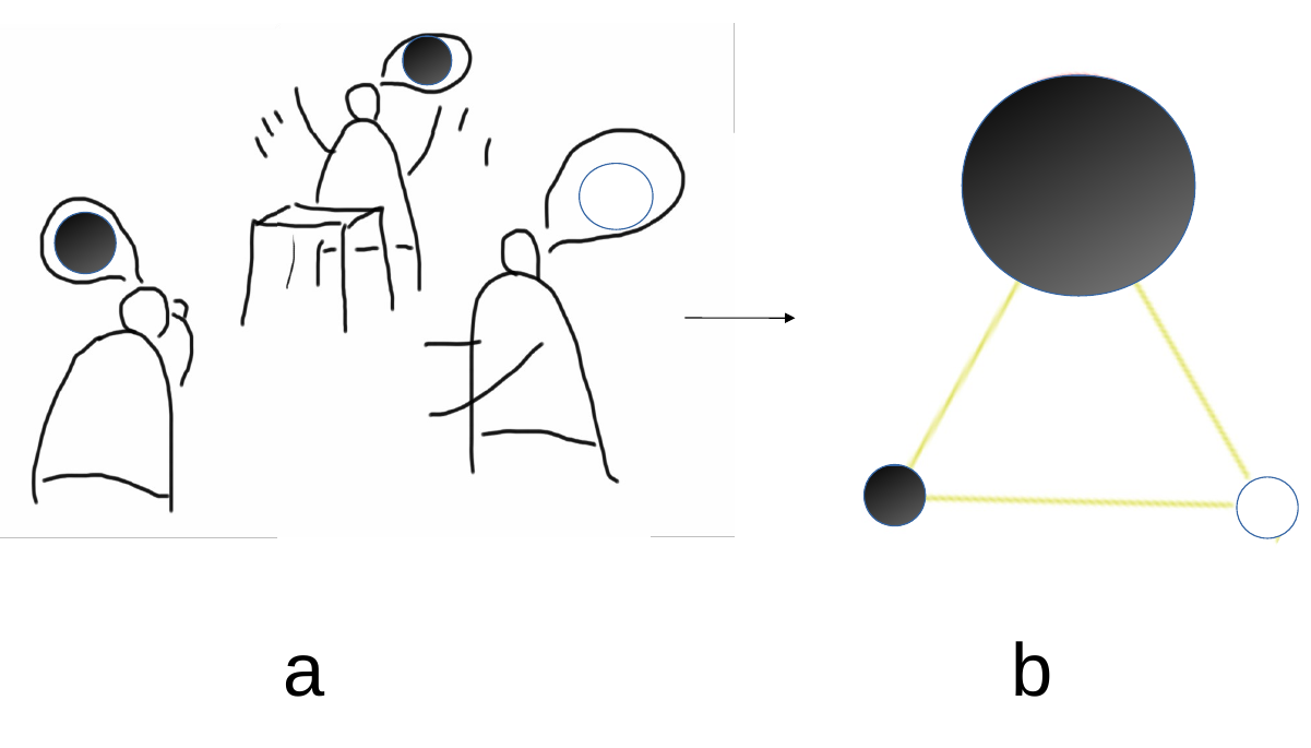An illustrative example of such a model, where each node has a discrete state, is shown in Fig. 1. Studies of analytical and numerical solutions for DN models become a topical issue in natural science [SS14, AHK⁺15b]. DN models have been successfully studied using graph theoretical approaches, algebraic groups properties of graphs, probability theory and Markov chains [Har69, Web12]. One such approach was explicitly demonstrated in [FW13], where a network is defined by the transformation matrix of a Markov chain. In particular, directed graphs can be interpreted in the sense that events are represented by nodes of the graph, and a directed line from one node to another indicates a positive probability of direct succession of these two events. Several of the concepts listed above have been successfully applied to describe a broad spectrum of various types of DN. However it is hard to develop a general theoretical framework for investigation of analytical solutions for DN models since they have structural differences.

Figure 1: Illustrative example of a dynamical network model: nodes represent humans (or separate communities). Links between nodes correspond to connections between humans, nodes size represents status of a human (or his/her importance in society) in the HOpS model. Links and states of the nodes can evolve in time.

Here I developed a new conceptual, stochastic Heterogeneous Opinion-Status model (HOpS model), presented in details in Section 2. The HOpS model admits to identify the main attributes of dynamics on networks and to study analytically the relation between topological network properties and processes taking place on a network. Another key point of the HOpS model is the possibility to study network dynamics via the novel parameter of heterogeneity. I show that not only clear topological network properties, such as node degree, but also the nodes’ status distribution play an important role in so-called opinion spreading and information diffusion on a network, Subsection 2.2. Furthermore, in Section 3 I propose an analytical method to study DN models demonstrating it on the HOpS model on networks with regular topologies. The analytic solutions are also extended by the numerical results from Subsection 3.4.

1.1 Motivation

The process of ”spreading out” of a substance is widely used in physics (particle diffusion), chemistry, sociology and others [Sok12, MJCB14]. Diffusion is a fundamental transport mechanism with countless examples in nature [GDGGG⁺12, TSIG14, BCC⁺13], which leave many open fundamental questions [BGM12, CL06]. The molecular nature of homogeneous diffusion was understood using new approach of Einstein to a random walk [Ein05]. The study of random walks on different structures such as regular lattices or, for instance, Cayley graphs [KB90], allows to understand how certain dynamical processes on networks take place, for instance, energy transfer, chemical reactions and transport problems. Moreover a variety of interesting mathematical problems arise from these studies [Shi12]. Spatial aspects of diffusion and advection processes were recently studied using the flow-networks approach presented in [RSGLHG14, TMM⁺16, KMT⁺16], and were discussed in details in Chapter III. Flow-networks are constructed from a discretisation of the advection-diffusion equation on regular grids, which helps to bridge the gap between the dynamics of the system and the topology of the corresponding correlation network. While the purpose of functional correlation networks (FCN) is to study data time-series or a dynamical systems from obtained topological properties of FCN, the purpose of so-called dynamical networks is to study processes on networks with a ”prescribed” topology, which can be in addition coupled with dynamics on a network [HZDG11]. It is clear that the combination (or in other words, adaptation) of non-trivial network topologies and dynamical processes on a network can produce rich dynamics. In many recent works on opinion and coalition formation [GK07, SS14, AHK⁺15b] dynamical adaptive networks were used as a prominent tool to analyze complex systems. One can define a variety of DN models on less regular networks, such as small-world networks and many others. Several statistical physics concepts were introduced to describe adaptive dynamics [CMPS09], which can also be applied to study social collective behavior. It is not necessary to justify that opinion formation processes play an important role in many aspects of our life [HLZ11, HK02a]. The last years have seen a clear rise of interest in collective phenomena emerging from the interactions between individuals in social structures. 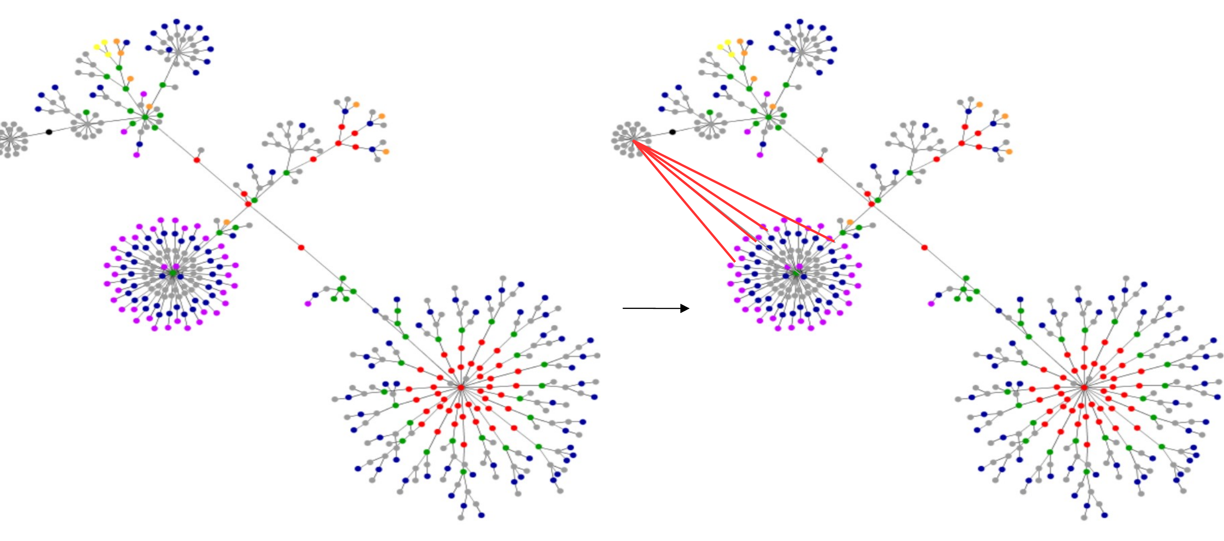Typically, society structure is represented as a network in mathematical approaches to this problem, where a link determines the connection between nodes, see Fig. 3. The ubiquitous real-world examples demonstrate, why it is important to model the information spread processes using DN models defined on networks:
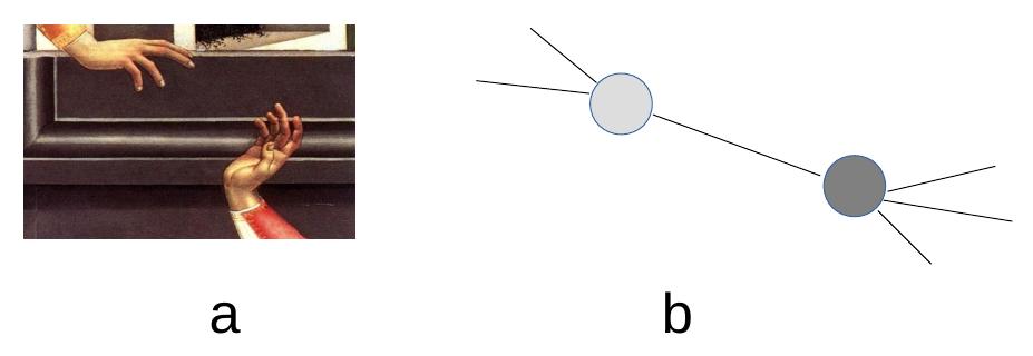
Example 1. Person $T$ lives in country $A$. $T$ is interacting every day with many people, but only from country $A$. After some time person $T$ gets a letter from another person from country $B$ with some information about himself (about person $T$). How is this possible? The reason is that some friend of person $T$, living in country $A$, traveled to country $B$ and spread the information about person $T$ to people from country $B$.
Example 2. One user with a few connections in some internet network wrote some news which were highlighted (”liked”) by some ”big hub” user in this social network. As a consequence, the news from this ”small user” are started to be spread by many other users, Fig. 2.
Nowadays thanks to the advantage of telecommunications, huge amount of data opens great opportunity to understand processes in society and estimate models of them, which was not possible before. But even before the accessibility of such data it was possible analytically to estimate cognitive properties of society. For instance, the sociologists P.Killworth and R.Dunbar defined and estimated a limit to the number of people with whom one can maintain stable social relationships, the so-called, Dunbar’s number [Dun92]. Development of social models including accessible applications to studies of ”flows” of opinion in society, riot behavior, innovation, strikes, voting and migration, have been extensively deliberated during the last decades [Gra78, GBBHM13, HS12]. From the series of seminal works it became clear that opinion ”flows” are mainly governed by the ”network hubs”, yet in [KGH⁺10] it was found that node degree is not the only characteristic of the ”node importance”. Instead, the most efficient spreaders are those located within the core of the network [Sei83]. There is a number of examples demonstrating that information propagation can be represented as ”flows” or ”opinion waves”. An illustrative example of such flows is the circulation of ideas among articles through citation network [KPH14, LG10].

Figure 2: Evolving twitter-network is shown in consequent time steps: at time step $t$ (a), and at time step $t+1$ (b), when several new connections are emerged in the network, highlighted in red.

Let us assume that each person is represented as a node in a network (toy representation of society). Before to come to the main research questions of this chapter, let us first compare the information spread model with a disease contagion model [LSS13], since the opinion spread could also be understood as a special type of contagion. In a recent work [RTH⁺15] the issue on difference between complex and simple contagion models has been addressed: in simple contagion models (SIR models) the most influential nodes are typically nodes with high degree and low clustering, while in complex contagion models the most influential nodes are typically characterized by low degree and high clustering. The main aspects, which differentiate various types of contagion spread mechanisms, can be conditionally separated into:
The mechanism of spreading, which is determined by properties of spreading, the stochastic or deterministic character of the information spreading, etc.
The mechanism of node state change, which determines how each node changes its state with dynamics on the network, including for example, resistance to change its current state.
In the series of recent works [SS14, GL14] it has been found that disease spread is more likely to be homogeneous among groups and depends mostly on the properties of the nodes, i.e. on mechanism of node state change. But on the other hand, the speed of opinion circulation strongly depends on the social group properties, society structure and the mechanism of spreading [ZG06, AHK⁺15a, BGB11, LGTR15]. Ties strength is important for social contagion which can be modeled as the status difference of the nodes [Gra78], one of possible examples is a weighted voter model [KSOM10]. This gave motivation to design a particular novel type of DN model, the HOpS model where a heterogeneity parameter plays an important role in dynamics of the model. The HOpS model I define in Subsection 2.2 after formulating types of dynamical network models and the research questions.

1.2 Research questions: graph dynamical models

Ultimately, in this chapter we shall deal with the following research questions to study DN models:
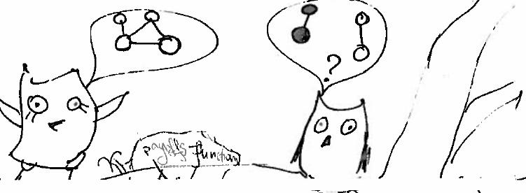
1. What are the conditions for a dynamical network model to come to a consensus state (defined further)? What is the speed of convergence towards the consensus? Is the consensus state unique, Fig. 4? How to characterise properties of phase space of dynamical network model analytically?
2. Is it possible to estimate the model evolution on a certain network topology without numerical simulations, for instance, using the transformation operator approach?
3. How is the underlying network topology reflected in the model’s dynamics? Are there any network topologies for which the model can be completely analysed? What are the effects of heterogeneous spread of opinion on the network?
All in all, I examine behavior of the HOpS model looking at these questions. Further I formulate a brief classification of DN models, Section 2, and methods overview to the existing methods in Subsection 2.1.

Figure 3: Connections between people have been topic of discussions besides artists and scientists since the ancient times. The fragment from Botticelli’s painting (a) illustrates a human interaction (b).

2 Dynamical network models classification

Any decent classification allows to find out, what has been done in a field and what remains undiscovered, however, recently new DN models on networks have not be structurally classified. Social, economic and biological networks can be modeled as dynamical network models or agent-based models [BPSDGA04, BR00, BCC⁺13, HN06, BMI⁺11], where each node has the possibility to change its state. Looking into real-world complex networks one can find many instances of networks whose states and topologies coevolve, i.e. they interact with each other and keep changing often over the same time scales, due to the system dynamics [SPS⁺13, HKDM16]. Depending on a type of a process being modeled, nodes of the dynamical network can have discrete and/or continuous evolving states, adaptive and/or non-adaptive strategies of evolution, and simultaneous switch of states of all nodes or a switch in a randomly picked node. Following such an approach divides properties of DN models of into classes, shown in Fig. 5.

Figure 4: Illustration of dynamical network model with different types of consensus states: total consensus (on the left) or separation into smaller groups (on the right), and in each of them consensus is reached.

2.0.1 Graph theoretical notations for dynamical network models

Let us describe the classification of DN models using graph theoretical notations, as it has been done in Chapter II for evolving networks. Let us denote a dynamical network model on an underlying graph $G=G(V,E)$ as $G(V,C(t),E)$, or simply as $G(t)$, where sets $V$ and $E$ are sets of nodes and edges correspondingly, number of nodes $|V|=N$, $C(t)$ is a set of nodes’ states at time step $t$, where a state of node $i$ is denoted by $c_{i}(t),i\in[1,N]$, where $c_{i}(t)$ takes values from a fixed set $Q$. For simplicity we fix sets $V$, $E$ and consider only finite subsets of integer numbers, which can have possible values. Let us denote a function $F$, acting on a set of nodes’ states. In fact, this can be also written in matrix notations. Let us denote $C(t)$ as a vector state of enumerated nodes’s states at time $t$ and $F$ is a matrix, defining transformations of nodes’ states (the exact form of this is given in Subsection 3.1). Then the evolution of dynamical network can be written according to a formula $F(C(t))=C(t+1)$, or in other words the evolution of a whole DN model on a static network topology can be written as:

$$F(G(V,C(t),E))=G(V,F(C(t)),E)=G(V,C(t+1),E).$$ (1)

Generally, each node of a DN model $G(t)$ may have several types of characteristics, instead of only one type $c_{i}(t)$. This can be encoded using additional set of nodes’ states $\{C^{1},...C^{k}\}$, each set $C^{j}$ for $j^{th}$ type of nodes’ characteristics, so that then a DN model would be denoted as $G(t)=G(V,C^{1}(t),...C^{k}(t),E)$.
As an example, let us consider an evolving DN model $G(t)=G(V,C(t),E)$ with fixed set of nodes, set of edges and boolean set of nodes’ states $Q=\{0,1\}$. Let a deterministic rule of $G(t)$ be: at each time step $t$ a state of each node $c_{i}(t),i\in[1,N]$ is changing its value to opposite value: $0\rightarrow 1,1\rightarrow 0$. If a node is changing its state to an opposite one a function $F$ can be written as $F(c_{i}(t+1))=(c_{i}(t)+1)mod2$.
Let us consider properties of functions, acting on set of nodes’ states. Let us assume that function $F_{i}$ acts on some subnetwork $G_{i}\subseteq G$. Assume, that a function $F$ is a composition of functions: $F=F_{1}F_{2}...F_{n}$. Notably, function $F_{i}$ does not necessarily commutate with function $F_{j}$, acting on another subnetwork $G_{j}\subseteq G$. Therefore, it is essential to distinguish the order in which functions are applied, $F_{i}F_{j}(G)$ or $F_{j}F_{i}(G)$.
Hence, characteristics of function $F$, such as in Eq. (1), typify the evolution of DN models. In particular, $F$ may act on a set of nodes’ states depending on edges evolution or independently on edges evolution (adaptive/non-adaptive networks); values of $C(t)$ may evolve in discrete or continuous time; $F$ may act on the whole network, or be applied to separate subgraphs of a network using synchronous or asynchronous update mechanism.
The model is evolving until a DN model reaches a final configuration, which can be either a consensus for the whole network or consensus, reached in disconnected small subnetworks, Fig. 4. Furthermore, in Subsection 3.1 I look at problems of DN models from another perspective of so-called sequential dynamical systems (SDSs) [BMR00, MM15], which helps to describe a discrete phase space of DN models.

Figure 5: Properties of dynamical networks models are divided into several classes depending on characteristics of functions, acting on node states, type of coevolution between nodes states and network topology.

2.1 Techniques to describe dynamical networks models

There exist various methods to study DN models, such as transfer operators approach, numerical approach to run models on ensembles of random topological graphs. Various random network models provide an efficient laboratory for testing various collective phenomena in statistical physics of complex systems, and are, on the other hand, tightly linked to statistical, topological properties of random matrices, for instance, vertex degree distribution, clustering coefficients, ”small world” structure and spectra of adjacency matrices [AGNV15, KK08, BBM08].
In order to illustrate one quite famous approach for studying dynamical system with discrete phase space let us consider the discrete transfer operators approach to study Moran model [Mor58]. At each time step a random individual of one of two types $A$ or $B$ is chosen for reproduction and a random individual is chosen for death; thus ensuring that the population size remains the same (the number of individuals is conserved). Here Moran process can be used to analyze variety-increasing processes such as mutation, as well as variety-reducing effects such as natural selection. This process describes the probabilistic dynamics in a population of finite constant size when two species $A$ and $B$ are competing for dominance. Now let us come to the transition matrix method to describe such systems.
The main idea of the transition matrix method is as follows. Let us consider system with discrete number of states, numerated by finite numbers $0s<i<N+1$. A phase space (or state space) is one-dimensional and discrete set $\{1,...,N\}$, where $N$ is the number of possible states (in other words, the cardinality of the phase space). The so-called transfer operator is thus represented by an $N\times N$ transition matrix $P$ acting on a vector in $\{0,1\}^{N}.$ Each entry $P_{i,j}$ of a transition matrix $P$ denotes the probability to go from state $i$ to state $j$. To understand the formulas for the transition probabilities one has to look at the definition of the process which states that always one individual will be chosen for reproduction and one is chosen for death, i.e. $P_{i,j}\in[0,1]$. Once all $A$ individuals have died out, they will never be reintroduced into the population since the process does not model mutations and thus $P_{1,1}=1$. For the same reason the population of $A$ individuals will always stay $N$ once they have reached that number and taken over the population and thus $P_{N,N}=1$. Then states $1$ and $N$ are called absorbing while the states $2,...,N-1$ are called transient. Analysing properties of transformation matrices, one can study possible states of the system.
Further I introduce the method based on analysis of transformation matrices, illustrating it on the Heterogeneous Opinion Status model (HOpS), Subsection 2.2.

2.2 Heterogeneous Opinion Status (HOpS) model setup

A novel dynamical network model, Heterogeneous Opinion Status (HOpS) model has the following properties, which allows to demonstrate analytical methods to characterise dynamics on networks.

Figure 6: Representation of the group of people with two possible opinions marked in black and white colors (a). Heterogeneous Opinion Status (HOpS) model representation of the group from three people (b), where the node status is represented by the node size.

The HOpS model setup

. Let us consider the network where each node $i$ has two variables: status and opinion. Status is fixed and is denoted by a finite number. Each node $i$ at time step $t$ has opinion $op_{i}(t)\in\{0,1\}$, $0$ is encoded as white color of the node and $1$ is black, Fig. 6, and $op_{i}(t)$ changes according to a stochastic rule representing the imitation of opinion.
Definition. Node $i$ is called an active node in the HOpS model, if node $i$ is randomly chosen at time-step $t$ with its random neighbor $j$ and then active node $i$ is changing its opinion $op_{i}(t)$ to opinion of its neighbor $op_{j}(t)$ with a fixed probability, dependent on the difference in statuses.
The algorithm of the HOpS model time step is given in Table 1. The dynamics is stochastic: at each time step a random individual $i$ chooses at random one of the neighbors, node $j$, and accepts the opinion of that neighbor with the probability $p=0.5\tanh(\sigma(st_{j}-st_{i}))+0.5$.

Table 1: Algorithm for the time step of the HOpS model

Phase of time step	Characteristics of each phase
1.	Randomly choose an active node $i$ from the network, Fig. 7.
2.	Randomly choose one neighbor of the active node $i$ - node $j$.
3.	Change the opinion of an active node $i$ to the opinion of
	node $j$ with probability $p=0.5\tanh(\sigma(st_{j}-st_{i}))+0.5$.
4.	Go to 1., iterating the whole time-step
	until a consensus state is reached.

Figure 7: Illustration of the time-step of the HOpS model: firstly, active node $i$ and its neighbor $j$ are randomly chosen; secondly, a state of an active node, opinion $op_{i}(t)$, is changed with probability $p$ depending on the status difference for nodes $i$ and $j$. A node status is encoded by a node size.

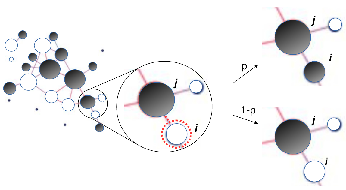
The opinion of an individual can evolve whenever some of the neighbors have opposite opinion. Consensus state, when all nodes have the same opinion of two equivalent opinion, either $0$ or $1$, is necessarily reached and is the absorbing state of this stochastic dynamics. Let us now formulate the HOpS model in notations from Subsection 2. The HOpS model is defined on a fixed graph $G(V,E)$ with a changing opinions of nodes, denoted by $Op(t)=(\{op_{i}(t)\}_{i\in[1,N]})$ and nodes statuses $St=(\{st_{i}\}_{i\in[1,N]})$. In other words, the HOpS model can be written as $G(V,Op(t),St,E)$.
The HOpS model input control parameters are:
1) a fixed set of nodes statuses $St$;
2) a distribution of initial nodes opinions at time step $t=0$ $Op(0)$, (this is discussed in details in Subsection 3.1, and moreover, this, on the first place, means that the system is non-ergodic);
3) a fixed underlying network topology $G(V,E)$. Moreover, a parameter $\sigma$ of a time step influences the HOpS dynamics, its role is discussed separately.
Note that a probability function of an opinion change was chosen to be a sigmoid function $0.5\tanh(\sigma(st_{j}-st_{i}))+0.5$, since a sigmoid function represents the increasing likelihood of imitation processes to take place with an increase in the status difference [TCH06, BCE⁺15, WDHL15]. By using a status difference, which can be either negative or positive, inside $\tanh$-function, we allow asymmetric relations between connected nodes: a node with a big status is influenced by the small node less than a node with a small status by a big node.
It is important to explain a meaning of a novel heterogeneity parameter of the HOpS model. The reason for introducing a new system’s ”heterogeneity” parameter can be seen from the following observation. Let us consider a group with one strong leader-dictator with a very high status, where the information transmission is directed from the group leader to others, in contrary to a homogeneous group. By the same token, it has been noticed in [Van99] that a hierarchy in society induces information spread from the leader to others more efficiently, than in structures where the hierarchical structure is less ”pronounced”. 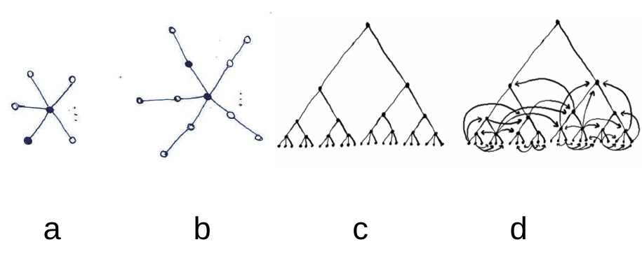Indeed, a tree-like hierarchical structure without loops Fig. 8 (a, b, c) admits smaller speed of convergence towards the consensus state than a network with loops, Fig. 8 (d), which is also linked to so-called geometrical frustration [MR06]. Note that in the HOpS model it is also assumed that when all statuses are the same, an active node changes its opinion to an opinion of its random neighboring node with probability $0.5$, and with equal probability opinion of an active node stays the same.
To summarize, the HOpS model is a particular kind of DN model with two prominent characteristics:
1. Each node $i$ has status $st_{i}$, which is as a characteristic of a so-called social influence. A distribution of nodes’ statuses introduces heterogeneity to the structure of a DN model and to a mechanism of a node state change.
2. Opinion change of each node $i$ is introduced by a threshold function and induces heterogeneity to a mechanism of an opinion spreading.
In Section 3 I present a new methodological framework for a class of dynamical network models. This methodics reveals analytic solutions for the HOpS model on symmetric networks. As the next step, I consider the HOpS model dynamics on random Erdős-Renyi networks [ER59], Subsection 3.4.

3 Results for Heterogeneous Opinion Status (HOpS) model

The analytical solutions for the Heterogeneous Opinion Status model for particular networks topologies are introduced in Subsection 3.2. The numerical results for the HOpS dynamics are described in Subsection 3.4.

Figure 8: Star-like networks: simple star $k=5$ (a), complex star (b). Hierarchical networks of different types: symmetric tree (c) tree with additional links between different hierarchal layers (d).

3.1 Analytic results for the HOpS model

There has been a variety of numerical studies on dynamics on networks, while analytic approaches to DN models analysis always have been lacking. Here I introduce a novel approach to study DN models using notations from theory of generalized cellular automata, Markov chains, and illustrating this approach on the HOpS model. The main idea of this technique is that for some model configurations, it is possible to calculate analytic solutions due to topological properties of these configurations. Let us call such configurations basic configurations. Which are these configurations? It is natural, first to consider basic network structures, particularly, a class of symmetric networks. Then further one can generalize model solutions for more complex underlying networks. The intuitive notion of a graph symmetry can be detected by graph measures [Hol06] and is characterized by features of group of graph automorphisms [Har69]. For symmetric networks this group is non-trivial [Gui15]. A formal definition for symmetric graphs is as follows (here the property of symmetry is defined for $G(V,E)$).

Definition. Two nodes $u$ and $v$ of a graph $G$ are similar, if for some automorphism $\alpha$ of $G$, $\alpha(u)=v$. A fixed point is not similar to any other point. Two lines $x_{1}=u_{1}v_{1}$ and $x_{2}=u_{2}v_{2}$ are called similar if there is an automorphism $\alpha$ of $G$ such that $\alpha(\{u_{1},v_{1}\})=\{u_{2},u_{2}\}$. Only graphs without isolated points are considered. A graph is point-symmetric, if every pair of points are similar; it is line-symmetric if every pair of lines are similar; and it is symmetric if it is both point-symmetric and line-symmetric [Har69].

Coming back to notations in Section 2, a state of the HOpS model at time step $t$ is denoted as $G(V,Op(t),St,E)$ and is determined by set of nodes’ states $Op(t)$. The opinion distribution $Op(t)=\{op_{i}(t),i\in[1,N]\}$ are components of a state vector at each time step. The state vector $Op(t)$ depends on a fixed statuses distribution $St$, a network topology $G(V,E)$, the initial opinions at $t=0$ time step $\{op_{i}(0),i\in[1,N]\}$ and on the time-step characteristics. The function $F$ describes a change of state-vector $F:G(V,Op(t),St,E)\rightarrow G(V,Op(t+1),St,E)$. Important to notice that function $F$ is contingent on the network topology.
It has been noticed that evolution of the processes on symmetric network topologies without loops has peculiar properties [KB90]. At the same time, topological properties of networks, such as symmetry, influence the main parameters, quantitatively characterize random walk on networks. These characteristics are, for instance, hitting time, cover time, mixing rate [Lov93]. The classical theory of random walks deals with random walks on simple, but infinite graphs, like grids, and usually studies their qualitative behavior: does the random walk return to its starting point with probability one or if it returns infinitely often? Or how structural or topological properties of networks are related to properties of transformation matrices of random walks [DGMS03, BLM⁺06]? An example of random walk properties is the mean quadratic derivation [KS08, TSGS12], the characteristic time, i.e. time after which the random walk has passed through all the nodes, defined for finite networks [BNL14].
With this in mind, first, I consider the HOpS model dynamics on symmetric networks without loops, for which I use the random walk theory [NV03, NR04, Sok12] and demonstrate the HOpS model results, conducted using picture of discrete-time random walk, Subsections 3.2 and 3.3.

3.2 The HOpS model dynamics on linear networks

As a starting point, I reveal analytic solutions for the HOpS model for particular kinds of symmetric networks: linear and star-like networks.

3.2.1 Analytic solution for the HOpS model on linear networks

Here I consider the HOpS model on linear networks, explained in two following propositions. Further term ”model” is meant to be the HOpS model if not stated otherwise.

Figure 9: The HOpS model on a linear network for $L=5$ nodes. A position of a border $x(t)$ between black and white nodes ($0<x(t)<L+1$) is considered as a random walker. The special initial condition: node statuses decrease linearly, nodes with different opinions are separated by a border. The HOpS model, starting from such initial condition, reaches one of two final stable states: all nodes have the same color.

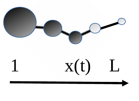
Let us consider the HOpS model on a linear network of length $L$. A space of all possible states of the HOpS model is denoted by $\mathbf{S}$, where each model state is fully described by opinion state vector is $Op(t)=(op_{1}(t),...,op_{N}(t))$, where $op_{i}(t)$ is opinion of a node $i$. Starting from random initial conditions a phase space $\mathbf{S}$ has $2^{L}$ possible distinguishable states.
Definition. A state of the DN model at time step $t$ is a state vector of opinions $Op(t)=(op_{1}(t),...op_{N}(t))$, when other model characteristics are fixed, such as status distribution $St=(st_{1},...st_{N})$ or network topology.
Let us now assume, that the model starts from a special initial model configuration: $Op(0)=(op_{1}(0),...op_{N}(0))=(0,0,...,0,1,...1)$ such that $x(t)$ left nodes are black, $L-x(t)$ right nodes are white. Moreover we assume, that nodes’ statuses are linearly decreasing from black to white nodes, Fig. 9, such that $\forall i\in[1,L-1]$ a status difference is fixed $(st_{i}-st_{i+1})=\Delta_{st}$.

Proposition I.
Starting from a special initial model configuration, all model states belong to a subspace $S^{\prime}$ of a phase space $\mathbf{S}$: $S^{\prime}\subset\mathbf{S}.$ Such a subspace is called an invariant subspace, since it fulfills the condition, that for any vector-state $Op(t)\in S^{\prime}:$ $Op(t+1)\in S^{\prime}$ $\forall t$. The number of states in this subspace $|S^{\prime}|=L$.
Proof: The number of states for the invariant subspace $S^{\prime}$ equals the number of all possible positions of the border $x(t)$ between black and white nodes. Starting from the special initial condition, the model is able to reach only a subspace of all system states, which belong to so-called invariant subspace. Hence, finding an invariant subspace of the system allows to describe all possible model states, or in other words, full phase space.

Proposition II.
The HOpS model dynamics with the special initial condition is equivalent to dynamics of an asymmetric bounded random walk $x(t)$ on a linear network.
Proof: Let us consider the probability of any black node to be converted into a white node is equivalent to $(0.5\tanh\sigma\Delta_{st}+0.5)$, where $\Delta_{st}=st_{i}-st_{j}$ is a fixed status difference. Then a state of the whole system is described just by position of a random walker $x(t)$. A probability of a random walk to drift to the right is denoted by $a=0.5\tanh(\sigma\Delta_{st})+0.5$ and probability of a random walk drift to the left is denoted by $b=1-a$. The model has two consensus states: when all nodes are either all black or all white. A probability of a random walker to reach the right border is equal to a probability of the HOpS model to come to a consensus when all nodes are black.

Here I refer back to the research questions on DN models behavior, Subsection 1.1, which are translated to the language of the random walk theory.

Bounded asymmetric random walk on a linear network
As it has been previously shown, the HOpS model dynamics on a linear network with a special initial configuration, as in Fig. 9, is described by a random walker $x(t)$. The probability of a random walker $x(t)$ to be shifted to the right equals $a$, and the probability of a random walker $x(t)$ to be shifted to the left equals $b$, as in Proposition II. Then probability $p(x(t+1)=i)$ for an asymmetric random walk $x(t)$ to be in position $i$ at time step $t+1$ can be written as:

$$p(x(t+1)=i)=\left\{\begin{matrix}0:|x(t+1)-x(t)|>1\\ a:x(t+1)-x(t)=1\\ b:x(t+1)-x(t)=-1\\ 1-a-b:x(t+1)-x(t)=0\end{matrix}\right\}$$ (2)

For convenience let us set $a+b=1$, which corresponds to a case when a random walker cannot stay on the same node. All together, this defines a transformation matrix $P$ with size $|P|=|S^{\prime}|\times|S^{\prime}|=L\times L$. The non-zero entries of a matrix $P$ are values on diagonals parallel to the main diagonal. Then an evolution equation for state vectors is defined by a tridiagonal right-stochastic matrix $P$:

$$Op(t+1)=Op(t)\cdot P$$ (3)

where $Op(t)$ is a state vector of opinions at time step $t$, and $P$ is a transformation matrix (column-stochastic) of a corresponding Markov chain. Hence, estimating asymptotics of the HOpS model is equivalent to Gambler’s ruin problem [Web12], which describes an asymmetric random walk on the integers $(1,...,L)$, with absorption at $1$ and $L$ nodes. Solving the Gambler’s ruin problem, we find solutions for the HOpS model on linear networks, as described below.

Proposition III.
Let us consider a bounded random walker on $[1,L]$ interval, starting from position $x_{0}$ with probability $a$ to walk to the right and probability $b$ to walk to the left. Then an asymptotic solution for an asymmetric bounded random walk on a linear network is given by a probability to hit the right border:

$$p(x_{0},a)=\frac{(a^{x_{0}}(1-a)^{L-x_{0}}-a^{L})}{((1-a)^{L}-a^{L})}.$$ (4)

Proof: Let a random walker be initially in position $x_{0}$. $p_{i}(j)$ defines a probability starting from $i$ to hit $j$. It is easy to see, that $p_{0}(0)=1,p_{0}(L)=0$ and correspondingly $p_{i}(0)=ap_{i-1}(0)+bp_{i+1}(0)$. Then a characteristic equation is

$$ax^{2}-x+b=(x-1)(ax-b)$$

which has roots $\{1,b/a\}$. For $a=b$ a random walker becomes symmetric. For $a\neq b$ a general solution $p(x_{0},a)$ is sum of the roots with the coefficients defined by the absorbing states at $1$ and $L$. Thus the probability of a random walker to hit one of the borders is:

$$p(x_{0},a)=\frac{(a^{x_{0}}(1-a)^{L-x_{0}}-a^{L})}{((1-a)^{L}-a^{L})}.$$ (5)

Moreover the Gambler’s ruin problem can be viewed as a special case of a first passage time problem, which asks to compute the probability that a Markov chain, initially in state, hits one fixed state before another.

Figure 10: Dynamics of the HOpS model on a linear network. $x_{0}\in[0,100]$ (horisontal axis) is initial number of black nodes and $a=0.5\tanh(\sigma\Delta_{st})+0.5$ (vertical axis). Colorbar corresponds to the probability $p(x_{0},a)$ for the system to come to one certain consensus, when all nodes are black, starting from $x_{0}$.

To sum up, the analytical results for the HOpS model on a linear network are:
(i) The HOpS model dynamics on a linear network is described by Propositions I, II, III. The quantitative characteristics of a phase space of the model are given in Proposition I. The formula (5) estimates the probability to reach a stable states of the model. From the formula (5) it is clear that $a=0.5\tanh(\sigma\Delta_{st})+0.5$ characterizes a speed of the model convergence towards a consensus state and $\sigma$ denotes scaling of a spreading process on a network.
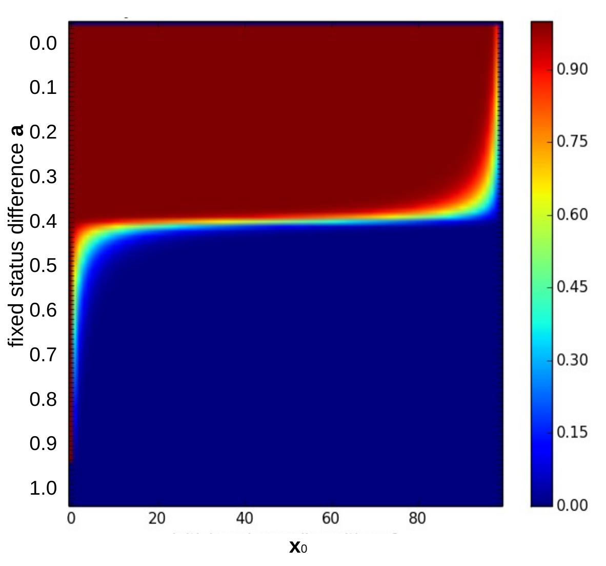
(ii) The analytic result of Proposition III is illustrated by the numerical result, Fig. 10. Each model simulation is made for values of $x_{0}$ and $a$. $x_{0}\in[0,100]$ corresponds to initial number of black nodes. $a=0.5\tanh(\sigma\Delta_{st})+0.5\in[0,1]$ characterizes the status difference between nodes. Then a probability to find the model in one certain stable state numerically corresponds to a ratio between a number of model simulations, which reach one certain possible consensus state to a number of total model simulations. The probability to find the model in its final state is marked by the color of each point $(x_{0},a)$, Fig. 10. Red region above the yellow curve on Fig. 10 corresponds to model simulations when the model converges towards a consensus, or in other words, a random walker reaches the right border. The curve separating red and blue regions is implicitly defined via relation $p(x_{0},a)=0.5$, Eq.(5), which gives the formula for the curve: $a^{x_{0}}(1-a)^{L-x_{0}}=2(1-a)^{L}-a^{L}$. Blue region below the curve corresponds to another absorbing state when the model reaches another stable state and, hence, a random walker with the characteristics from that region never reaches the right border.
(iii) The schematic diagram of a discrete phase space of the HOpS model on linear networks is presented in Fig. 11. The arrows on the diagram correspond to transitions between different model states. Topology of a diagram of the model on a linear underlying network is trivial, yet it illustrates how one can represent a part of a phase space of DN models. For more convoluted underlying network topologies the model phase space has more complex structure, as it is shown in Subsection 3.3.

Figure 11: Schematic diagram characterizes a phase space of the HOpS model on a linear network for a special initial condition. The phase space is presented as a sequence of states and transitions between them, shown by arrows. Here the phase space is shown only for the HOpS model with a special initial state: $L-x(0)$ nodes from the left border are black, and $x(0)$ nodes from the right border are white at time step $t=0$.

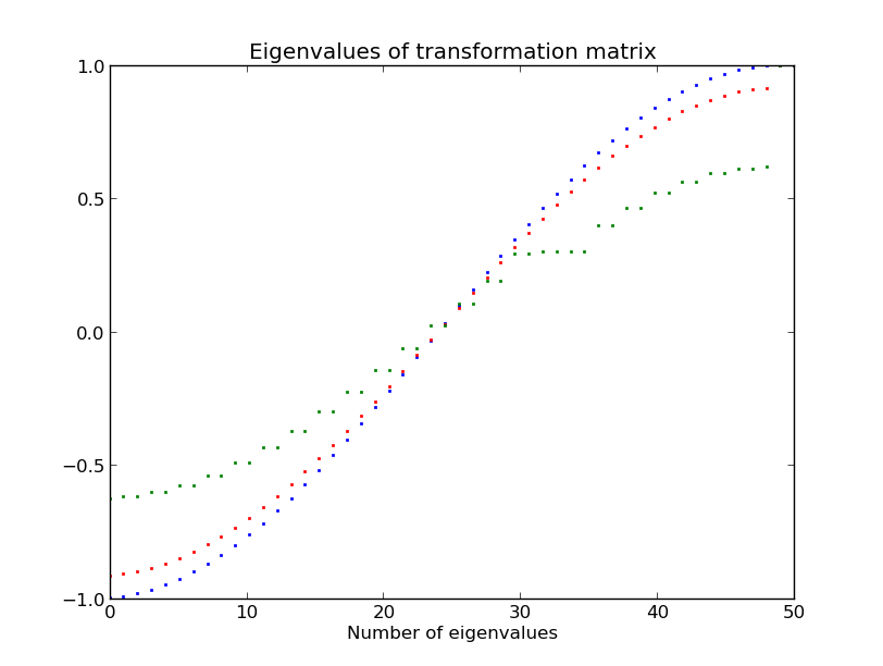
Additionally to the analytical results, spectra of transformation matrices $P$ for various values of parameter $a=0.5\tanh(\sigma\Delta_{st})+0.5$ are calculated in Fig. 12. Interestingly, spectral properties of a transformation matrix and mixing properties of the system, described by this transformation matrix, are related. The spectral gap, by definition, is a gap between the largest and the second largest eigenvalues of a matrix. As can be observed from Fig. 12, the spectral gap is smaller for larger $a$ values ($a>0.5$), which means that larger values of parameter $a$ correspond faster mixing times of the system [CNK⁺14] and forces faster reaching the consensus than for smaller $a$ values. Translating this to the language of the HOpS model, the bigger the status difference $\Delta_{st}$, the faster the equilibrium state is reached. This property is also related to the mixing time of the corresponding Markov chain and it is also known as Cheeger Inequality [Lov93].

Figure 12: Spectrum of a transformation matrix for the HOpS model on a linear network for $L=50$. Larger spectral gaps are observed for larger parameter values $a=0.5\tanh(\sigma\Delta_{st})+0.5$ values, as the result, this gives faster convergence towards the consensus. Spectra for $a=0.5$ is blue dashed line, for $a=0.7$ - red dashed line, for $a=0.9$ - green dashed line.

3.3 The HOpS model on star-like networks

After demonstrating analytical solutions for the HOpS model dynamics on a linear network, the next step is to consider the HOpS model on more general symmetric structures, such as star-like networks, Fig. 8 (a,b). First I consider particular types of star-like networks.
Definition. A simple star is a network with one central node and $k$ ”leaves” i.e. one-node edges, attached to a central node, Fig. 8 (a). A simple star is a tree-like network with tree depth $1$.
It is important to emphasize, that the definition of a star-like network highlights two main differences in comparison with a linear network: (1) We have to cope with a more complex network topology. Any type of dynamics on the star-like graph is obviously not equivalent to dynamics in the case of linear network [KSGN15]. (2) As the consequence, the over-all complexity of the model dynamics on star-like network is larger. However, as it is found below, the analytic techniques to describe the model dynamics on simple star-like networks are originated from the framework for the linear network case, Subsection 3.2.

Figure 13: Equal states of the HOpS model on a simple star with $k=3$ leaves: two states are equivalent iff in both states the central node has the same color and the number of nodes-leaves with identical color is the same.

3.3.1 The model dynamics on a simple star network

Let us first consider a simple star network with $k$ one-node ”leaves” and one central node. The number of the system’s states for random initial conditions is $|\mathbf{S}|=2^{k+1}.$ Now assume, that all ”leaves” of a simple star network have some fixed statuses $st_{i}=s$, $i=\{1,...k\}$, and a central node has a higher status $st_{k+1}=s+\Delta s$ where $\Delta s$ is a parameter of status difference. As we saw, the HOpS model on a linear network, the existence of the invariant subspace simplifies the description of the whole discrete phase space $\mathbf{S}$ of the system. Remarkably, there is no non-trivial invariant subspace inside space $\mathbf{S}$, for simple star-like networks. If there existed such an invariant subspace $S^{\prime}$, then there would be a special initial condition, i.e. a vector-state $Op(t)$ from a subspace $Op(t)\in{S}^{\prime}$ such that for $\forall t$ a transformation $P$ results in: $Op(t)P\in{S}^{\prime}$. But using finite enumeration method [HP67] it is easy to see that there is no such initial conditions, in contrary to the case for the HOpS model on a linear network. Simply speaking, the reason for this is that a structure of a group of symmetries for a star-like network is more complex than a group of symmetries for a linear network. Nevertheless, it is possible to ”simplify” a space $\mathbf{S}$ using a natural algebraic technique to induce the parametrization on a space $\mathbf{S}$ [Vin01]. The main advantage of the parametrization is that it allows to change the structure of the space $\mathbf{S}$, so that the parametrized space ${S^{*}}$ has an invariant subspace, while the corresponding ”initial” space $\mathbf{S}$ doesn’t. Note also that nodes-leaves of a star network do not interact with each other. This means that the probability of transition between a state with $n$ black leaves and a state with $(n-1)$ black leaves is independent from $n$. Let us first consider elements of the space $\mathbf{S}$, the states of the model at time steps $t_{i}$ and $t_{j}$ with corresponding state vectors $Op(t_{i})$ and $Op(t_{j})$. In order to parameterize a full space of states $\mathbf{S}$ I introduce a natural equivalence relation between states.

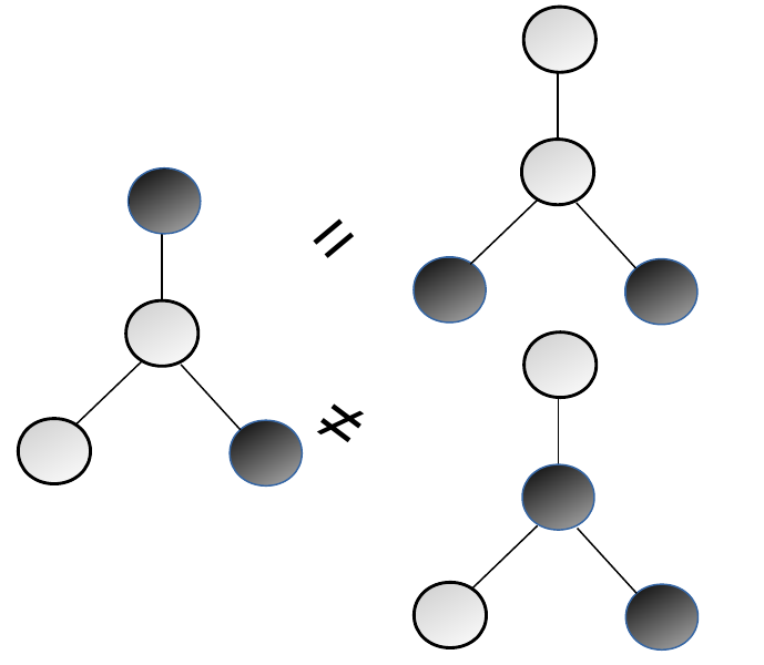
Definition. I call two states of the HOpS model on the star-like network equivalent, as in Fig. 13, $Op(t_{i})\sim Op(t_{j})$ iff:
in both states the central node has the same color;
in both states the number of nodes-leaves with white color is the same.

Using such an equivalence relation, we are now ready to parametrize the space of states $\mathbf{S}$. Later on I come back to this issue, discussing equivalence of DN models. Parameterized space $S^{*}$ is then defined as $S^{*}=\mathbf{S}/\sim$. Notably, a group of equal states of the space $\mathbf{S}$ corresponds to a state of the space $S^{*}$. Let us call states of space $S^{*}$ macro-states, in order to distinguish them from states of ”initial” phase space $\mathbf{S}$. In the following proposition I describe equivalent macrostates of the HOpS model from the algebraic point of view.

Proposition IV.
All equivalent macro-states of the model on a star-like network form a group $\Pi^{\prime}$ in respect to the operation of a permutation.
Proof. Let us consider equivalent states $Op(t_{i})$ and $Op(t_{j})$ from the whole discrete phase space $\mathbf{S}$ of the model on a star-network. Each node has a Boolean value $op_{i}\in\{0,1\}$. Then the proposition follows from the fact that vector states $Op(t_{j})$ and $Op(t_{j})$ belong the same macro-state in the parametrized space $S^{*}$. In another words, two states $(op^{1}_{1}(t_{i}),...op^{1}_{k+1}(t_{i}))$ and $(op^{2}_{1}(t_{i}),...op^{2}_{k+1}(t_{i}))$ of space $\mathbf{S}$ belong to the same macro-state of space $S^{*}$, iff there exists such a permutation $\pi$:

$$\exists\pi\in\Pi^{\prime}:(op^{1}_{1}(t_{i}),...op^{1}_{k+1}(t_{i}))=(\pi(op^{2}_{1}(t_{i}),...op^{2}_{k+1}(t_{i}))).$$ (6)

Without loss of generality, let us enumerate a central node as the $1^{st}$ node with opinion, denoted by $op_{1}(t)$. Then a permutation on states of nodes $\pi\in\Pi^{\prime}$, which transforms two equal states between each other, has a property:
$\pi(op_{1}(t_{i}),op_{2}(t_{i}),...op_{k+1}(t_{i}))=(op_{1}(t_{i}),\pi(op_{2}(t_{i})),...,\pi(op_{k+1}(t_{i})))$,
so that opinion of a central node stays the same. In other words, the group $\Pi^{\prime}$ consists of such permutations for which a value of a central node is preserved.
Interestingly, a subgroup $\Pi^{\prime}$ of a group $\Pi$ of all permutations of a set of $(k+1)$ numbers is isomorphic to a subgroup of symmetric group. This follows from the Caley theorem [Bab95], which states that every finite group $\Phi$ is isomorphic to a subgroup of a symmetric group $Sym(\Phi)$. This property of a group of permutations gives intuition behind structure of permutations.
Furthermore, an opinion of a randomly chosen active node $i$ evolves in time as: $op_{i}(t+1)=(op_{i}(t)+1)mod2$.
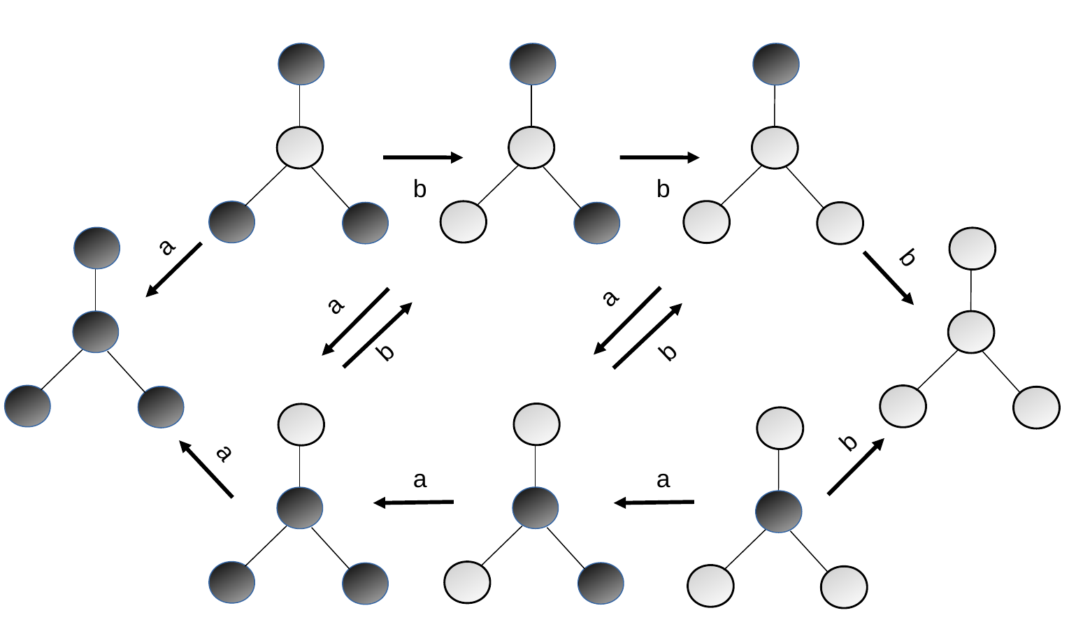
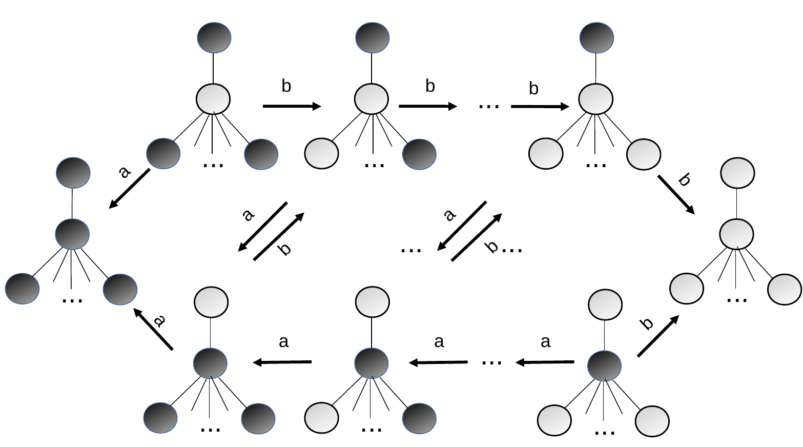
The discrete phase space of the model on a star-like network is shown in a schematic way in Fig. 14, where each model configuration can be transported to another configurations with probabilities $a=0.5\tanh(\sigma\Delta_{st})+0.5$ or $b=1-a$. In fact, the structure of such graphical diagram is not occasional, and is connected to algebra of processes [BH01] and sequential dynamical networks [BMR00].

3.3.2 Sequential dynamical systems

Definition. Sequential dynamical systems (SDSs) are constructed from the following components: (1) A finite underlying graph $G$ with vertex set $V=\{1,2,...,N\}$. Depending on the context the graph can be directed or undirected. (2) A state $x_{w}$ for each vertex $i$ of $G$ taken from a finite set of values $K$. The system state is the $N$-tuple $x=(x_{1},x_{2},...,x_{N})$, and $x[i]$ is the tuple consisting of the states associated to the vertices in the 1-neighborhood of $i$ in $G$ (in some fixed order). (3) A vertex function $f_{i}$ for each vertex $i$. The vertex function maps the state of vertex $i$ at time $t$ to the vertex state at time $t+1$ based on the states associated to the 1-neighborhood of $i$ in $G$. Stochastic Sequential dynamical system (SSDS) has the same components as SDS accept that the update rule has stochastic component [MM15].
Sequential dynamical systems may be thought of as generalized cellular automata, the main difference between SDS and the DN model is that SDS has a deterministic update rule. Similarly to the case of the HOpS model a structure of a phase space of SDS is governed by topological properties of an underlying graph $G$, vertices’ states $\{f_{i}\}_{i\in[1,N]}$, and the so-called update sequence $\omega$ defining the transformation of vertices’ states. Note that for deterministic SDSs, each state in its phase space can be transformed only to one state, while for stochastic SDSs (SSDS) each state does not necessarily have only one possible state, where it can be transformed. In the definition of DN model, a transformation $F$ is defined on a set of all possible states $\Gamma=\{G(V,Op(t),St,E),t\in[0,\infty)\}$ so that $F:\Gamma\rightarrow\Gamma$. Note, that a transformation matrix of a function $F$ is denoted by $P$.Another useful notion from theory of SDSs is a digraph of SDS, a graph, where each link of digraph is associated with a transition between model states in discrete phase space of SDS. In the following proposition I explain the connection between SDSs and the HOpS model.

Proposition V.
A phase space of the HOpS model is associated with a digraph of some stochastic SDS.
Proof of this short proposition follows from the definition of a stochastic SDS.

A phase space of stochastic SDS can be understood as a weighted underlying graph, where weights denote probabilities of transformations between states of the system.

Definition. The basin of attraction of an attractor in a discrete phase space of SDS is the set of all states that eventually end up on this attractor, including the attractor states themselves. The size of the basin of attraction is the number of states belonging to it.

In case of the HOpS model on a finite networks a basin of attractor consists of states, which can be transformed to absorbing states (consensus states). The HOpS model on a linear network or on a star graph has two possible absorbing states. Which of these states will be reached depends on the initial condition of the model.

Definition. The state space $\Omega$ of the HOpS model (or of any finite DN model) is the finite directed graph (digraph), where an edge exists between states, if they can be transformed from one to another.
The following proposition describes the HOpS model from the point of view of discrete finite dynamical systems [MR01].

Proposition VI.
Since the set of states of the HOpS model (in principle, of any finite DN model) on a finite underlying network is finite, any directed path must eventually enter a directed cycle, called a limit cycle.
Proof: Directed paths in full space of the HOpS states $\Gamma$ correspond to iterations of a function $F$ on the model’s states or to state, at the beginning of the path. Then because there is a finite number of possibilities of paths, at some point path of states comes back to the state, where it started. In other words, because we deal with the map between the set of all states $\{0,1\}^{N}\rightarrow\{0,1\}^{N}$ and the sets of possible states are finite, for any given initial condition it must have either a unique fixed-point or a limit cycle, otherwise the set would have to be non-finite.

Definition. Two SDSs are called isomorphic if there exists a digraph isomorphism between the phase spaces of these SDSs. These SDSs are stably isomorphic if there exists a digraph isomorphism between their limit cycle graphs.

Finally, let us come back to the HOpS dynamics. We call two DN network models equivalent in terms of the HOpS model, if their digraphs of phase spaces of these models are isomorphic. Then Propositions I-VI can be extended to describe the HOpS model dynamics on a broader class of underlying networks, than just on linear and star-like networks, but also on underlying networks, for which the HOpS model phase space has non-trivial invariant subspace. The digraph of the HOpS model phase space, Fig. 14, has a symmetric structure, which, in fact, is connected to symmetric properties of underlying networks. In particular, the diagram in Fig. 14 exposes two absorbing states, transient states and moreover contains a limit cycle. Hence, SDSs theory provides a promising tool to describe DN models. In the following subsection I analyze the HOpS model in terms of transformation matrices.

3.3.3 Transformation matrix approach for the HOpS model on star-like networks

Let us now consider a transformation matrix $P_{k}$ for the macro-states of the HOpS where $k$ is the number of leaves of the simple star-like network. The size of matrix $P_{k}$ is defined by the parametrized space $S^{*}$, as I showed in the case of the model on linear networks. Therefore a size of the transformation matrix $|P_{k}|$ for a star-like network is $(2k+2)\times(2k+2)$, where $2k+2$ is the total number of states for the model on a star-network with $k$ leaves. This can be easily seen from the diagram Fig. 14. As an example, I consider the HOpS model on a simple star network for $k=3$ leaves. which has a transformation matrix $|P_{3}|=8\times 8$. The structure of $P_{3}$ can be reordered in such a way that the first and the last matrix rows correspond to absorbing states of the system and rows $i\in[2,2k+1]$ of the matrix $P_{k}$ correspond to transient states. The elements of $P_{3}$ are rearranged in such a way that the nonzero matrix elements $a,b$ are parallel to the main diagonal. Then the matrix has a form:

$$P_{3}=\begin{pmatrix}1&0&0&0&0&0&0&0\\ a&0&0&0&0&b&0&0\\ 0&a&0&0&0&0&b&0\\ 0&0&a&0&0&0&0&b\\ a&0&0&0&0&b&0&0\\ 0&a&0&0&0&0&b&0\\ 0&0&a&0&0&0&0&b\\ 0&0&0&0&0&0&0&1\\ \end{pmatrix}$$ (7)

In general, if the simple star-like network has $k$ leaves, the transformation matrix $P_{k}$ can be transformed to a Toeplitz matrix. This Toeplitz matrix has nonzero elements on four diagonals parallel to the main diagonal, which correspond to transition probabilities $a,b$ between states of the model:

$$P_{k}=\begin{pmatrix}1&0&0&0&...&0&0&...&0&0\\ a&0&0&0&...&b&0&...&0&0\\ 0&a&0&0&...&0&b&...&0&0\\ &&&&...&&&\\ a&0&0&0&...&b&0&...&0&0\\ 0&a&0&0&...&0&b&...&0&0\\ &&&&...&&&\\ 0&0&0&0&...&0&0&...&0&1\\ \end{pmatrix}$$ (8)

where the distance between nonzero elements $a$ and $b$ elements in each row equals $k+1$. In analogy with the case of the HOpS model on a linear network knowing the transformation matrix $P_{k}$ of the system allows to find a stationary solution, an absorbing state of the model. It can be found as a vector state $Op(t\rightarrow\infty)$ for $t\rightarrow\infty$ for the HOpS model on a star-like network by the evolution equation, Eq. (3): $Op(t+1)=Op(t)P_{k}$. Then using geometric series we find

$$Op(t\rightarrow\infty)=Op(0)(I-P_{k})^{-1}$$

where $Op(0)$ is an initial state of the parameterized space $S^{*}$, $I$ is an identity matrix.

Figure 14: Phase space of the HOpS model on a simple star with $k=3$ leaves (top), arbitrary number of leaves (bottom). The arrows between each two states of the HOpS model represent transition probabilities, which equal $a$ and $b$ correspondingly, Subsection 3.1.

Symmetric networks have nontrivial group of automorphisms, i.e. it consists of more than from one element by the definition). This fact also causes that the invariant subspace of the full space of states is nontrivial, therefore a symmetry is emerged in the structure of the phase space. As a result, it is possible to describe network state using schematic diagrams, such as in Fig. 14. Although in this section I considered linear and star-like networks, some analytical results from Subsection 3.1 are generalizable for solutions on the HOpS model dynamics on more general topologies. One example of such topology is a complex star network with $k$ ”long leaves”, chains formed by $l$ nodes attached to a central node, Fig. 8 (b). Ultimately, presented methodological framework gives possibility to perform analysis of other DN models for network’s topologies such as linear combination of star-networks trees, circular networks, fully connected graphs and others, which is discussed in the Outlook Section.

3.3.4 Consensus state for the HOpS model on a star networks

Let us investigate the probability to reach the consensus state for the HOpS model on a star graph from the arbitrary initial condition. The HOpS model dynamics is described by the recursion formulas:

$$W_{n}=\frac{1}{N+1}\,\frac{N-n}{N}\,B_{n}+\frac{N-n}{N+1}\,W_{n+1},\\ B_{n}=\frac{1}{N+1}\,\frac{n}{N}\,W_{n}+\frac{n}{N+1}\,B_{n-1}$$ (9)

where $W_{n}$ denotes the probability for a model to be in a state with a white center, i.e. central node has opinion $0$, being surrounded by $n$ black nodes, while $B_{n}$ the probability for a model to be in a state with the black center, i.e. central opinion has opinion $1$, being surrounded by $n$ black nodes. Eqs. (9) are obtained by analogical observations to [KR03], where the consensus time is estimated from the master equation for the majority rule model. Here we note that equations 9 have asymmetry, which leads to the asymmetric property of solutions. Eqs. (9) can be easily solved for small $N$. I i.e. for $N=2$ we get $W_{0}=\tfrac{8}{35},W_{1}=\tfrac{12}{35},W_{2}=1,B_{0}=0,B_{1}=\tfrac{2}{35},B_{2}=\tfrac{13}{35}$. For bigger $N$ the transformation matrix method is needed.

3.3.5 Analytical findings for the HOpS model on a star-like network

To summarize, the main analytical findings for the HOpS model on a star-like network are:
(i) The HOpS model dynamics on star-like networks is described by Propositions IV and V, the discrete phase space of the model is demonstrated in the schematic diagram, Fig. 14. As it can be seen from this digraph, transient states of the HOpS model form cycles. Moreover, since some random regular graphs are locally approximated as trees, then solution for the HOpS model dynamics on trees (or particularly, on star-like graphs) can give intuition for model solution on the whole graph.
(ii) The evolution of the HOpS model can be described using the transformation matrix framework. An example of a transformation matrix equations for the HOpS model on a star network is illustrated in Eq. (7).
(iii) The general framework for studying a dynamical model on networks can be formulated as the following. Firstly, one needs to find possible symmetries of the underlying network itself and to identify the invariant subspace of the full space of model states, as it has been demonstrated for a particular cases of networks in Proposition I. Then a phase space (or a part of a phase space) of a model can be represented as a digraph of SDSs, see Propositions V and VI. This would give qualitative characteristic of a model evolution. Secondly, one needs to estimate the transformation matrix as it was shown in Subsection 3.3, which gives quantitative characteristic of a model evolution.

3.4 Numerical results for the HOpS model on random networks

The analytic solutions for DN models on special networks topologies were discussed in details in Section 3. Further step is to get an intuition for the numerical results of the HOpS model on random network topologies. Apart from inherent topological properties of random networks, these networks usually have a self-induced structure, which influences the flow of transport [HK02b]. This gives additional motivation to investigate random network models in the context of the HOpS model.

3.4.1 The HOpS model dynamics on random Erdős-Renyi networks

The random network type of the interest is random Erdős-Renyi (ER) network $G_{N,p}$ on $N$ nodes [ER59]. As it was already defined in Chapter II, each possible edge between two vertices is present in ER network with independent probability $p$, and absent with probability $1-p$. It is important to mention that each realisation of ER network with particular $p$ value is only a particular member of the entire statistical ensemble of random ER graphs. Hence, studying such model dynamics one needs to consider statistical ensemble of random networks instead of one particular random network realisation. Up till now in this chapter the space of model states of the HOpS model was mostly analyzed analytically. Underlying structure of ER networks is more complex than in ”deterministic” symmetric networks, which leads to more intricate organisation of a phase space. I numerically examine behavior of the HOpS model by changing the model control parameters, specifically, the ER network randomization parameter $p$. Then for each specific value of a control parameter $p$ I calculate the number of time steps till consensus is reached, hence I estimate so-called waiting or relaxation time. Notably, relaxation times for the HOpS model on symmetric deterministic networks with analytically estimated transformation matrix $P$ can be estimated as a spectral gap of a matrix $P$, while waiting time for ER networks here is estimated numerically.

The waiting time for the HOpS model on ER networks. The waiting time as the function of an ER parameter $p$ for random configurations of network is shown in Fig. 15. The HOpS model dynamics is simulated on each realisation of $300$ ER networks $G(N,p)$ for $N=90$ nodes for each value $p$. The initial opinion distribution is randomized at each model run. The numerical simulations are performed until the HOpS model reaches a consensus. The waiting time in Fig. 15 reaches the plateau for a value $p\approx 0.15$. In order to discuss the properties of the waiting time it is useful in parallel to examine the characteristics of ER networks.
Interestingly, ER networks have rich geometric properties, while being constructed by quite a simple rule. Let us consider the process of slow increase of ER parameter $p$. First, for low $p$ values ER network $G_{N,p}$ consists from disconnected small components. Note that in each of such small component the consensus state of the HOpS in average is reached faster than on the whole fully connected network $G_{N,p}$ [KRBN13]. Then if $p$ increases a newly introduced links start to appear more often between two disjoint clusters rather than between two nodes in the same cluster, and at some point the giant component will be formed. For larger $p$ disconnected components of $G_{N,p}$ will form a bigger predominantly tree-like network, which still has a low link density, but spans more nodes than ER network for smaller $p$. Therefore the waiting time for the HOpS model on such tree-like network is expected to increase in comparison to the waiting time for the HOpS model on a tree-like component with lower link density. When $p$ continues to increase at some point ER network forms a fully connected component. A fully connected component has high connectivity, hence the waiting time starts to decrease in comparison to the waiting time for smaller $p$ values. To summarize, for $p$ values larger than $p_{c}=1/N$, clusters in $G_{N,p}$ are small and tree-like [New03]. For $p>p_{c}$, a ”giant” cluster is emerged, with all other components having size $O(\log N)$ [KS12]. Geometrically the percolation phenomenon in ER networks looks as the following: first for small $p$ there are just ”seeds”, (small disconnected clusters of ER network $G(N,p)$). Then for larger $p$ these ”seeds” emerge into a ”forest” (a giant component), which is formed from cycles and trees linked together. The waiting time is affected by such reformation of components size distribution, which is discussed in the following remark.

Figure 15: The waiting time for the HOpS model on random Erdős-Renyi networks depending on the probability of link creation $p$ is shown in subplot (a). Random realisations of the model are made for fixed parameters: $N=90$ nodes, $T_{max}=100000$, $\sigma=1$, with random statuses distribution for each model realisation. The waiting time (vertical axis) is calculated for each parameter $p$ (horisontal axis). Log-log plot for the standard deviation/mean values of the waiting time is shown in subplot (b). A peak for a parameter of ER network $p\approx 0.15$ indicates the transition.

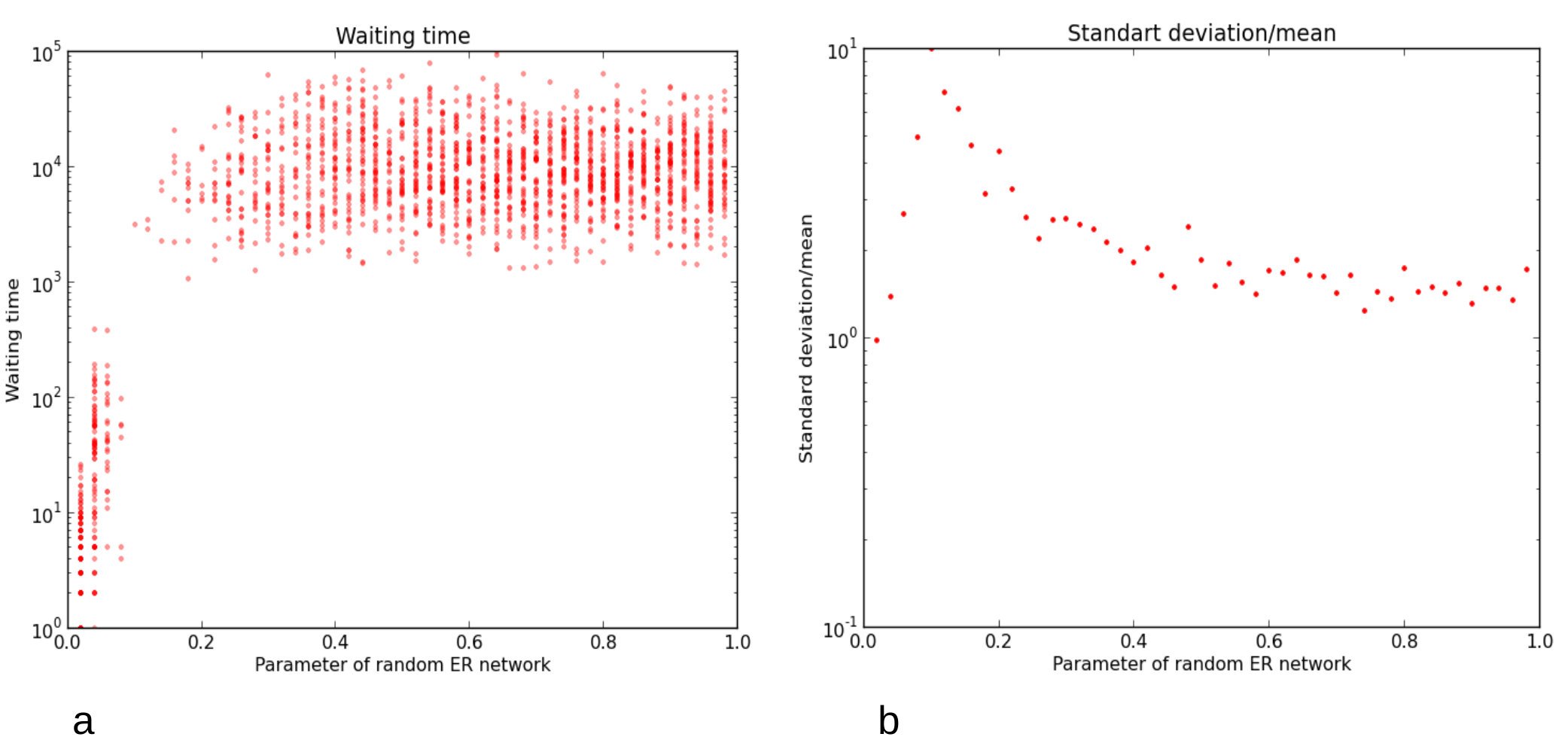
Remark. The waiting time for the HOpS model dynamics on ER networks exhibits a transition in respect to the value of the ER parameter $p$. As it has been found numerically in Fig. 15, the transition of the waiting time is observed for value $p\approx 0.15$. Some intuition for the analytical explanation to this observation is the following. Let us consider an ordinary diffusion process on a densely connected network [GLS⁺11]. Let $T_{d}$ denote the waiting time till complete spreading through all nodes. Now let us compare $T_{d}$ with the waiting time $T_{c}$, which is the time of a complete spreading for a less densely connected network, which still forms a joined component, on the same set of nodes. Intuitively it is clear that the density of network connections influences the characteristics of dynamic process on networks, giving $T_{d}<T_{c}$, if other parameters, such as number of nodes in a network or network connectivity, are kept the same for both networks. In general, dynamics of DN models on arbitrary underlying structures is a challenging question, which is discussed further in the Conclusions and the Outlook Section.

4 Conclusions and further directions

The main conclusions of this chapter are enumerated below:

• 1. A novel Heterogeneous OPinion-Status Model (HOpS) is introduced in this chapter. The model dynamics on specific network topologies is described by Propositions I-VI.

• 2. The HOpS model serves as a revealing test case for the new theoretical framework to describe a phase space of a discrete state model on networks, Section 3. The model setting links problems of discrete DN models with theory random walks [KS11]. For symmetric networks a phase space of the model is regular, Figs. 11 and 14. The approach to analyze a phase space of the HOpS model can be extended for more complex underlying network topologies using theory of sequential dynamical systems and the master equation approach [Mor13, KRBN13].

• 3. A theory of SDSs suggests a possible approach to study dynamics of DN models. This can be significant both theoretically and practically for a case of more general underlying graph structures. The novel approach to study DN models has its drawbacks, for instance, growing entanglement of a phase space with increasing complexity of a topological structure of the underlying network.

• 4. The numerical results for the model on Erdős-Renyi (ER) random graphs are given in Subsection 3.4. The transition for a waiting time is observed for ER networks for an approximate value of ER randomization parameter $p\approx 0.15$, Fig. 15.

• 5. The effects of heterogeneous spread of opinion on a network in the HOpS model were studied: particularly, it has been found that the speed of convergence towards the consensus state for the HOpS model on star-like graphs is affected by the heterogeneity parameter, introduced by a status distribution of nodes. The network topology and the heterogeneity parameter are reflected in the HOpS model dynamics. As the result, the speed of convergence for the HOpS model on linear and star-like networks depends on the status difference parameter $\Delta_{st}$, Fig. 12.
  Since HOpS model is a model of evolving opinion in heterogeneously distributed environment of statuses, one may ask, whether the results of the model dynamics are relevant for the real processes in society? The HOpS model dynamics can be an approximation of some complex systems, however the main motivation to study it was to deal with new types of dynamics and analysis methods. Most of the real world systems can be represented as complex DN models, therefore development of general techniques to study such models is a topical issue in physics.

Figure 16: Change of nodes states in the HOpS model on a tree-like network can be presented as ”random walkers”, traveling on the network: at each time step one node has a probability to change its state.

4.0.1 Outlook

The outlook includes open questions and generalizations of ideas from IV chapter:
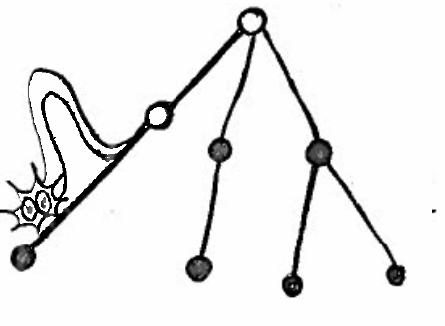
1. What is the general method to find analytical solutions for the HOpS model on networks with arbitrary topology? A method to analyze DN models, Section 3.1, has one particular limitation - the requirement of a regular or acyclic structure of an underlying network, like a tree-like structure on Fig. 16. However, the analytical solutions for the HOpS model can be extended in a quite straightforward way further for networks with more complex topologies. Also, in order to find the HOpS model solutions on asymmetric networks, adjacency matrices of asymmetric networks can be tackled as perturbed adjacency matrices of symmetric networks. It seems potentially interesting, to relate schematic diagrams, Fig. 14, with theory of group-reduced distributions [Gui15] and the algebraic Galois theory for SDSs [LP01]. Additionally theory of Coxeter and Sylow’s groups could serve as promising instrument for theoretical description of SDSs [Mor13, Mac07], and also for analytical description of DN models.

2. Which are further directions to study the HOpS model? One potential generalization of the model is to introduce the co-evolution of network topology and nodes’ states. One of the possible model modification: let us call node $i$ an active node, if the random walk on the network is traveling on the network through this node. Additionally to this, some problems, such as to find analytical solutions for DN dynamics are closely interrelated to problems from the random walks theory [NV03, Sin82, KS11], particularly, random walks on weighted directed networks and on circular networks with randomly added short-cuts. Moreover, a novel heterogeneity parameter of the HOpS model can be introduced to any DN model, it induces an interesting complex dynamics, as it has been illustrated for linear and star-like networks.

3. How the HOpS and voter models are interrelated? From the schematic diagram of the phase space of the model states of the HOpS model, Fig.14, it can be seen that in the HOpS model a node can change color from white to black even even if most of the nodes in its surrounding are white (this is not possible in the voter model, where the mean opinion of the surrounding nodes defines the change of the opinion). These models can be described using general framework [KS11, Gle13, IIBH05, Red02].

4. Which are possible applications of kinetic approach to the HOpS model? There is a link between the HOpS model on a linear network from random initial conditions and the domain walls dynamics. The analytic solutions for the domain walls dynamics are known as a sum of Bessel functions [KRBN13]. A domain wall is simply a border between nodes with different opinions in the HOpS model. For instance, in Fig. 10 there is one domain wall on a linear network, since there is only one edge between two sets of nodes with different opinions. In the language of domain walls it is clear that the HOpS model on a linear network with several domain walls has more complex dynamics rather than the HOpS model with only one domain wall. The homogeneous case, when a domain wall can move symmetrically with equal probabilities on a linear network, is also known as Sinai’s random walk, or ”quenched disorder” phenomenon [KB97, Sin82].
Furthermore, the methods, developed in Chapters II, III for evolving networks and flow-networks, can be applied in order to quantify changes in generalizations of DN models on coevolving networks.

References

- [ADGK+08] Alex Arenas, Albert Diaz-Guilera, Jurgen Kurths, Yamir Moreno, and Changsong Zhou. Synchronization in complex networks. Physics Reports, 469(3):93–153, 2008.
- [AGNV15] Vladik Avetisov, Alexander Gorsky, Sergei Nechaev, and Olga Valba. Spontaneous Symmetry Breaking and Phase Coexistence in Two-Color Networks. Arxiv, pages 1–9, 2015.
- [AHK+15a] Ashton Anderson, Daniel Huttenlocher, Jon Kleinberg, Jure Leskovec, and Mitul Tiwari. Global Diffusion via Cascading Invitations: Structure, Growth, and Homophily. Proceedings of the 24th International Conference on World Wide Web, 2015.
- [AHK+15b] Sabine Auer, Jobst Heitzig, Ulrike Kornek, E Scholl, and Jürgen Kurths. The Dynamics of Coalition Formation on Complex Networks. Scientific reports, 5(13386), 2015.
- [Bab95] Laszlo Babai. Automorphism groups, isomorphism, reconstruction. Handbook of Combinatorics, pages 1447–1540, 1995.
- [BBM08] Gerrit Baxter, R A Blythe, and A.J McKane. Fixation and consensus times on a network: a unified approach. Physical review letters, 101(25):258701, 2008.
- [BCC+13] A. Barrat, C. Cattuto, V. Colizza, F. Gesualdo, L. Isella, E. Pandolfi, J. F. Pinton, L. Ravà, C. Rizzo, M. Romano, J. Stehlé, a. E. Tozzi, and W. Van den Broeck. Empirical temporal networks of face-to-face human interactions. European Physical Journal: Special Topics, 222(6):1295–1309, 2013.
- [BCE+15] Felix Brandt, Vincent Conitzer, Ulle Endriss, Jerome Lang, and Ariel D. Procaccia. Introduction to Computational Social Choice. Handbook of Computational Social Choice, pages 1–29, 2015.
- [BGB11] Vitaly Belik, Theo Geisel, and Dirk Brockmann. Natural Human Mobility Patterns and Spatial Spread of Infectious Diseases. Physical Review X, 1(1):1–5, 2011.
- [BGM12] Eli Barkai, Yuval Garini, and Ralf Metzler. Strange kinetics of single molecules in living cells. Physics Today, 65(8):29–35, 2012.
- [BH01] Ed Brinksma and Holger Hermanns. Process Algebra and Markov Chains. Euro Summer School on Trends in Computer Science, 2090:183–231, 2001.
- [BLM+06] Stefano Boccaletti, Vito Latora, Yamir Moreno, Mario Chavez, and D. Hwang. Complex networks: Structure and dynamics. Physics Reports, 424(4-5):175–308, 2006.
- [BMI+11] Nicola Botta, A. Mandel, C. Ionescu, M. Hofmann, D. Lincke, S. Schupp, and C. Jaeger. A functional framework for agent-based models of exchange. Applied Mathematics and Computation, 218:4025–4040, 2011.
- [BMR00] C.L. Barrett, H.S. Mortveit, and C.M. Reidys. Elements of a theory of simulation II: sequential dynamical systems. Applied Mathematics and Computation, 107(2-3):121–136, 2000.
- [BNL14] Moreno Bonaventura, Vincenzo Nicosia, and Vito Latora. Characteristic times of biased random walks on complex networks. Phys Rev E Stat Nonlin Soft Matter Phys, 89(1):012803, 2014.
- [BPSDGA04] Marián Boguñá, Romualdo Pastor-Satorras, Albert Díaz-Guilera, and Alex Arenas. Models of social networks based on social distance attachment. Physical Review E - Statistical, Nonlinear, and Soft Matter Physics, 70(5 2):1–8, 2004.
- [BR00] Stefan Bornholdt and Thimo Rohlf. Topological Evolution of Dynamical Networks: Global Criticality from Local Dynamics. Physical Review Letters, 84(26):6114–6117, 2000.
- [CL06] Ronald R. Coifman and Stéphane Lafon. Diffusion maps. Applied and Computational Harmonic Analysis, 21(1):5–30, 2006.
- [CMPS09] Claudio Castellano, Miguel Munoz, and Romualdo Pastor-Satorras. The non-linear q-voter model. Physical Review E, 80:041129–1–8, jul 2009.
- [CNK+14] Mickaël David Chekroun, J David Neelin, Dmitri Kondrashov, James C McWilliams, and Michael Ghil. Rough parameter dependence in climate models and the role of Ruelle-Pollicott resonances. Proceedings of the National Academy of Sciences of the United States of America, 111(5):1684–90, mar 2014.
- [DGMS03] Sergei N. Dorogovtsev, Alexander Goltsev, Jose F. F. Mendes, and A N Samukhin. Spectra of complex networks. Physical review. E, Statistical, nonlinear, and soft matter physics, 68(4 Pt 2):046109, 2003.
- [Dun92] Robin Dunbar. Neocortex Size as a Constraint on Group-Size in Primates. Journal of Human Evolution, 22(6):469–493, 1992.
- [Ein05] Albert Einstein. On the Motion of Small Particles Suspended in a Stationary Liquid, as Required by the Molecular Kinetic Theory of Heat. Annalen der Physik, 322(8):549–560, 1905.
- [ER59] Paul Erdös and Alfred Rényi. On random graphs I. Publ. Math. Debrecen, 6:290–297, 1959.
- [FW13] Mark Freidlin and Alexander Wentzell. Mathematics Subject Classification. Number 3. Springer, 2013.
- [GBBHM13] Sandra González-Bailón, Javier Borge-Holthoefer, and Yamir Moreno. Broadcasters and Hidden Influentials in Online Protest Diffusion. American Behavioral Scientist, 57(0):943–965, 2013.
- [GDGGG+12] Sergio Gomez, Albert Diaz-Guilera, J. Gomez-Gardenes, Yamir Moreno, C.J. Perez-Vicente, and Alex Arenas. Diffusion dynamics on multiplex networks. Physical review letters, 110 (2):1–6, 2012.
- [GK07] Thilo Gross and Ioannis G. Kevrekidis. Robust oscillations in SIS epidemics on adaptive networks: Coarse-graining by automated moment closure. page 6, feb 2007.
- [GL14] Rumi Ghosh and Kristina Lerman. The Impact of Network Flows on Community Formation in Models of Opinion Dynamics. Arxiv, pages 1–13, jul 2014.
- [Gle13] James P. Gleeson. Binary-state dynamics on complex networks: Pair approximation and beyond. Physical Review X, 3(2):1–20, 2013.
- [GLS+11] Rumi Ghosh, Kristina Lerman, Tawan Surachawala, Konstantin Voevodski, and Shang-Hua Teng. Non-Conservative Diffusion and its Application to Social Network Analysis. arXiv preprint, feb 2011.
- [Gra78] Mark Granoventer. Threshold models of collective behavior. American Journal of Sociology, 83(6):1420–1443, 1978.
- [GS09] Thilo Gross and Hiroki Sayama. Adaptive Networks. Springer Berlin Heidelberg, 2009.
- [Gui15] David Guichard. An Introduction to Combinatorics and Graph, 2015.
- [Har69] Frank Harary. Graph theory. Perseus Books, Michigan, 1969.
- [HK02a] Rainer Hegselmann and Ulrich Krause. Opinion Dynamics and Bounded Confidence. Simulation, 5(3):2, 2002.
- [HK02b] Petter Holme and Beom Jun Kim. Vertex overload breakdown in evolving network. Physical Review E, 65:1–8, 2002.
- [HKDM16] Jobst Heitzig, Tim Kittel, Jonathan F. Donges, and Nora Molkenthin. Topology of sustainable management of dynamical systems with desirable states: from defining planetary boundaries to safe operating spaces in the Earth system. Earth System Dynamics, 7(1):21–50, 2016.
- [HLZ11] Jobst Heitzig, K. Lessmann, and Yong Zou. From the Cover: Self-enforcing strategies to deter free-riding in the climate change mitigation game and other repeated public good games. Proceedings of the National Academy of Sciences, 108(38):15739–15744, 2011.
- [HN06] Petter Holme and M. Newman. Nonequilibrium phase transition in the coevolution of networks and opinions. Physical Review E, 74(5):056108, nov 2006.
- [Hol06] Petter Holme. Detecting degree symmetries in networks. Physical Review E - Statistical, Nonlinear, and Soft Matter Physics, 74(3), 2006.
- [HP67] Frank Harary and Ed Palmer. Enumeration of finite automata. Information and Control, 10(5):499–508, 1967.
- [HS12] Jobst Heitzig and Forest W. Simmons. Some chance for consensus: Voting methods for which consensus is an equilibrium. Social Choice and Welfare, 38(1):43–57, 2012.
- [HZDG11] C Huepe, G Zschaler, Do Anne, and Thilo Gross. Adaptive network models of swarm dynamics. New Journal of Physics, 13(073022), 2011.
- [IIBH05] Dmytro Ivaneyko, J Ilnytskyi, Bertrand Berche, and Yu Holovatch. Criticality of the random-site Ising model : Metropolis , Swendsen-Wang and Wolff Monte Carlo algorithms. Arxiv, 8(1):149–162, 2005.
- [KB90] G. Kohler and Alexander Blumen. Variance of random walks on Cayley trees : application to the trapping problem. Journal of physics A, 5611, 1990.
- [KB97] Paul Krapivsky and Eli BenNaim. Domain statistics in coarsening systems. Physical Review E, 56(4):3788–3798, 1997.
- [KGH+10] Maksim Kitsak, Lazaros K. Gallos, Shlomo Havlin, Fredrik Liljeros, Lev Muchnik, H. Eugene Stanley, and Hernan a. Makse. Identifying influential spreaders in complex networks. Nature Physics, 6(11):36, 2010.
- [KK08] Paul Krapivsky and Dmitri Krioukov. Scale-free networks as preasymptotic regimes of superlinear preferential attachment. Physical Review E - Statistical, Nonlinear, and Soft Matter Physics, 78:1–11, 2008.
- [KMT+16] Hannes Kutza, Nora Molkenthin, Liubov Tupikina, Norbert Marwan, Jonathan F Donges, Jurgen Kurths, and Reik V Donner. Edge anisotropy and the geometric perspective on flow networks. Chaos, 2016.
- [KPH14] Tobias Kuhn, Matja Perc, and Dirk Helbing. Inheritance Patterns in Citation Networks Reveal Scientific Memes. Physical Review X, 4:041036 1–9, 2014.
- [KR03] P L Krapivsky and Sid Redner. Dynamics of Majority Rule in Two-State Interacting Spin Systems. Physical Review Letters, 90(23):238701, 2003.
- [KRBN13] Pavel L. Krapivsky, Sid Redner, and Eli Ben-Naim. Kinetic view on statistical physics, volume 53. Cambridge University Press, 2013.
- [KS08] Joseph Klafter and Igor M Sokolov. Anomalous diffusion spreads its wings. Physics world, 18(8), 2008.
- [KS11] Jossi Klafter and Igor M. Sokolov. First Steps in Random Walks. From Tools to Applications. Oxford University Press, 2011.
- [KS12] Michael Krivelevich and Benny Sudakov. The phase transition in random graphs: A simple proof. Random Structures & Algorithms, pages 1–9, 2012.
- [KSGN15] Justus A. Kromer, Lutz Schimansky-Geier, and Alexander B. Neiman. Emergence and coherence of oscillations in star networks of stochastic excitable elements. Physical Review E, 042406, 2015.
- [KSOM10] Masahiro Kimura, Kazumi Saito, Kouzou Ohara, and Hiroshi Motoda. Learning to Predict Opinion Share in Social Networks. Proceedings of the 23rd AAAI Conference on Artificial Intelligence, 2010.
- [LG10] Kristina Lerman and Rumi Ghosh. Information Contagion: an Empirical Study of the Spread of News on Digg and Twitter Social Networks. ACM Transactions on Embedded Computing System, 2010.
- [LGTR15] Maxime Lenormand, Bruno Gonçalves, Antònia Tugores, and José J. Ramasco. Human diffusion and city influence. Journal of The Royal Society Interface, 12(109):20150473, 2015.
- [Lov93] Laslo Lovasz. Random Walks on Graphs : A Survey. Royal Society Mathematical Studies, 2(Volume 2), 1993.
- [LP01] Reinhard Laubenbacher and Bodo Pareigis. Equivalence Relations on Finite Dynamical Systems. Advances in Applied Mathematics, 251:237–251, 2001.
- [LSD+10] Renaud Lambiotte, Roberta Sinatra, J. C. Delvenne, Tim S. Evans, M. Barahona, and Vito Latora. Flow graphs: interweaving dynamics and structure. Physical Review E, 84:4, dec 2010.
- [LSS13] Hartmut H. K. Lentz, Thomas Selhorst, and Igor M Sokolov. Unfolding accessibility provides a macroscopic approach to temporal networks. Phys. Rev. Lett., 110, 2013.
- [Mac07] Matthew Macauley. On Enumeration of Conjugacy Classes of Coxeter Elements, 2007.
- [MJCB14] Ralf Metzler, Jae-Hyung Jeon, Andrey G. Cherstvy, and Eli Barkai. Anomalous diffusion models and their properties: non-stationarity, non-ergodicity, and ageing at the centenary of single particle tracking. Phys. Chem. Chem. Phys., 16(44):24128–24164, 2014.
- [MM15] Matthew Macauley and Henning S Mortveit. Cycle Equivalence of Finite Dynamical Systems Containing Symmetries. Cellular Automata and Discrete Complex Systems, 8996:70–82, 2015.
- [Mor58] Patrick A P Moran. Random processes in genetics. Mathematical Proceedings of the Cambridge Philosophical Society, 54(01):60–71, 1958.
- [Mor13] Henning S. Mortveit. Introduction to sequential dynamical systems, volume 53. 2013.
- [MR01] Henning S Mortveit and Christian M Reidys. Discrete, sequential dynamical systems. Discrete Mathematics, 226(2001):281–295, 2001.
- [MR06] Roderich Moessner and Arthur P. Ramirez. Geometrical frustration. Physics Today, 59(2):24–29, 2006.
- [MRS+16] Michael E. Mann, Stefan Rahmstorf, Byron A. Steinman, Martin Tingley, and Sonya K. Miller. The Likelihood of Recent Record Warmth. Scientific Reports, 6:19831, 2016.
- [New03] Mark E. J. Newman. The structure and function of complex networks. SIAM Review, 45(2):167–256, 2003.
- [NR04] Jae Dong Noh and Heiko Rieger. Random Walks on Complex Networks. Physical Review Letters, 92(11):118701–1, 2004.
- [NV03] Sergei Nechaev and Raphael Voituriez. Random walks on three-strand braids and on related hyperbolic groups. Journal of Physics a-Mathematical and General, 36(1):43–66, 2003.
- [Red02] Sid Redner. A Guide to First-Passage Processes, volume 70. 2002.
- [RSGLHG14] Vincent Rossi, Enrico Ser-Giacomi, Cristóbal López, and Emilio Hernández-García. Hydrodynamic provinces and oceanic connectivity from a transport network help designing marine reserves. Geophysical Research Letters, 41(8), 2014.
- [RTH+15] Sara Brin Rosenthal, Colin R Twomey, Andrew T Hartnett, Hai Shan Wu, and Iain D Couzin. Revealing the hidden networks of interaction in mobile animal groups allows prediction of complex behavioral contagion. Proceedings of the National Academy of Sciences, 112(15):4690–4695, 2015.
- [SBD+15] Will Steffen, Wendy Broadgate, Lisa Deutsch, Owen Gaffney, and Cornelia Ludwig. The trajectory of the Anthropocene : The Great Acceleration. The Anthropocene Review, 2015.
- [Sch98] Hans-Joachim Schellnhuber. Discourse: Earth System Analysis – The Scope of the Challenge. Springer-Verlag, Berlin, earth syst edition, 1998.
- [Sei83] Stephen B. Seidman. Network structure and minimum degree. Social Networks, 5(3):269–287, 1983.
- [Shi12] Shiryaev Albert N. Probability, volume XXXIII. Springer, 2012.
- [Sin82] Yakov Sinai. The limiting behavior of a one-dimensional random walk in a random medium. Theory of probability and its applications, 27(2):256–268, 1982.
- [Sok12] Igor M. Sokolov. Models of anomalous diffusion in crowded environments. Soft Matter, 8(35):9043, 2012.
- [SPS+13] Hiroki Sayama, Irene Pestov, Jeffrey Schmidt, Benjamin James Bush, Chun Wong, Junichi Yamanoi, and Thilo Gross. Modeling complex systems with adaptive networks. jan 2013.
- [SS14] Hiroki Sayama and Roberta Sinatra. Social Diffusion and Global Drift in Adaptive Social Networks. Physical Review E, 91(032809):1–4, 2014.
- [TCH06] Arne Traulsen, Jens Christian Claussen, and Christoph Hauert. Coevolutionary dynamics in large, but finite populations. Physical Review E, 74(1):011901, jul 2006.
- [TMM+16] Liubov Tupikina, Nora Molkenthin, Norbert Marwan, P O Box, and Palma De Mallorca. Correlation networks from flows. The case of forced and time-dependent advection-diffusion dynamics. PLoS ONE, pages 0153703–1–11, 2016.
- [TSGS12] Felix Thiel, Lutz Schimansky-Geier, and Igor M. Sokolov. Anomalous diffusion in run-and-tumble motion. Physical Review E - Statistical, Nonlinear, and Soft Matter Physics, 86(2):1–4, 2012.
- [TSIG14] Michael V. Tamm, V. I. Stadnichuk, A. M. Ilyina, and Denis S. Grebenkov. Overlap of two Brownian trajectories: Exact results for scaling functions. Physical Review E, 89(4):042137, 2014.
- [Van99] Piet Van Mieghem. Topology information condensation in hierarchical networks. Computer Networks, 31(20):2115–2137, 1999.
- [Vin01] Vinberg Ernest Borisovich. Algebra. Graduate Studies in Mathematics, 2001.
- [WDHL15] Marc Wiedermann, Jonathan F Donges, Jobst Heitzig, and Wolfgang Lucht. Macroscopic description of complex adaptive networks co-evolving with dynamic node states. Physical Review E, 91(052801), 2015.
- [Web12] Richard Weber. Markov Chains: lecture notes, 2012.
- [ZG06] Damián H. Zanette and Santiago Gil. Opinion spreading and agent segregation on evolving networks. Physica D: Nonlinear Phenomena, 224(1-2):156–165, dec 2006.