h KA-TP-27-2017
Gauge-independent Renormalization of the
N2HDM

Abstract

The Next-to-Minimal 2-Higgs-Doublet Model (N2HDM) is an interesting benchmark model for a Higgs sector consisting of two complex doublet and one real singlet fields. Like the Next-to-Minimal Supersymmetric extension (NMSSM) it features light Higgs bosons that could have escaped discovery due to their singlet admixture. Thereby, the model allows for various different Higgs-to-Higgs decay modes. Contrary to the NMSSM, however, the model is not subject to supersymmetric relations restraining its allowed parameter space and its phenomenology. For the correct determination of the allowed parameter space, the correct interpretation of the LHC Higgs data and the possible distinction of beyond-the-Standard Model Higgs sectors higher order corrections to the Higgs boson observables are crucial. This requires not only their computation but also the development of a suitable renormalization scheme. In this paper we have worked out the renormalization of the complete N2HDM and provide a scheme for the gauge-independent renormalization of the mixing angles. We discuss the renormalization of the $\mathbb{Z}_{2}$ soft breaking parameter $m_{12}^{2}$ and the singlet vacuum expectation value $v_{S}$. Both enter the Higgs self-couplings relevant for Higgs-to-Higgs decays. We apply our renormalization scheme to different sample processes such as Higgs decays into $Z$ bosons and decays into a lighter Higgs pair. Our results show that the corrections may be sizeable and have to be taken into account for reliable predictions.

1 Introduction

Even after the discovery of the Higgs boson by the LHC experiments ATLAS [1] and CMS [2] there remain many open questions that cannot be solved within the Standard Model (SM). This calls for New Physics (NP) extensions, which feature predominantly extended Higgs sectors. The precise investigation of the Higgs sector has become an important tool in the search for NP, in particular since its direct manifestation through the discovery of new non-SM particles remains elusive. Among the beyond-the-SM (BSM) Higgs sectors those with singlet and doublet extensions are particularly attractive as they are at the same time rather simple and compatible with custodial symmetry. The 2-Higgs-doublet model (2HDM) [3, 4, 5] is interesting due to its relation to supersymmetry and has been extensively studied and considered as a possible benchmark model in experimental analyses. It features 5 physical Higgs bosons, 2 CP-even and 1 CP-odd neutral states and a charged Higgs pair. The next-to-minimal 2HDM (N2HDM) is obtained upon extension of the 2HDM by a real singlet field with a $\mathbb{Z}_{2}$ parity symmetry. It contains in its symmetric phase a viable Dark Matter (DM) candidate. The N2HDM has been the subject of numerous investigations, both in its symmetric [6, 7, 8, 9, 10, 11, 12, 13, 14, 15, 16, 17, 18, 19] and in its broken phase [20, 21, 22]. The Higgs sector of the latter consists after electroweak symmetry breaking (EWSB) of 3 neutral CP-even scalars, 1 pseudoscalar and a charged Higgs pair. With the Higgs mass eigenstates being superpositions of the singlet and doublet fields the N2HDM entails an interesting phenomenology, namely the possibility of a light Higgs boson, which is not in conflict with the experimental Higgs data in case of a sufficiently large singlet admixture so that its couplings to SM particles are suppressed. The enlarged Higgs sector together with the possibility of light Higgs states allows for cascade Higgs-to-Higgs decays that provide alternative production channels for the heavier Higgs bosons and also give access to the trilinear Higgs self-couplings. Their measurement provides important insights in the understanding of the Higgs mechanism [23, 24, 25].

Obviously, any NP extension has to comply with the relevant theoretical and experimental constraints. Thus, also the N2HDM has to provide at least one Higgs boson with a mass of 125 GeV compatible with the LHC data on the discovered Higgs resonance [26]. The additional Higgs bosons must not violate the LHC exclusion limits. The compatibility with the electroweak (EW) precision data has to be guaranteed as well as the compatibility with $B$-physics and low-energy constraints. The symmetric N2HDM furthermore has to provide a DM candidate that complies with the DM observables. From the theoretical point of view, the N2HDM Higgs potential has to be bounded from below, its vacuum has to be the global minimum and perturbative unitarity has to be respected. In [21], part of our group investigated the N2HDM in great detail with respect to these constraints. The allowed parameter space was determined and the phenomenological implications were investigated. In the course of this work the model was implemented in HDECAY [27, 28]. The generated code, N2HDECAY [29], computes the N2HDM Higgs decay widths and branching ratios including the state-of-the-art higher order QCD corrections and off-shell decays. The model was furthermore included in ScannerS [30, 31] along with the theoretical conditions and the available experimental constraints, which then allowed to perform extensive parameter scans for the model. In [22], the work was extended and we compared the N2HDM to other NP extensions with the aim to work out observables that can be used to distinguish between various well-motivated BSM Higgs sectors by using collider data.

Since the discovered Higgs bosons behaves very SM-like [32, 33, 34, 35], the search for NP in the Higgs sector requires on the theoretical side precise predictions for parameters and observables including higher-order (HO) corrections. In the framework of the 2HDM, some of the authors of this work provided an important basis for the computation of HO corrections in the 2HDM by working out a manifestly gauge-independent renormalization of the two 2HDM mixing angles $\alpha$ and $\beta$, which is also numerically stable and process independent [36]. These angles, which diagonalise the neutral CP-even and the neutral CP-odd or charged Higgs sectors, respectively, enter all Higgs couplings so that they are relevant for Higgs boson phenomenology. We completed the renormalization of the 2HDM Higgs sector in [37] by investigating Higgs-to-Higgs decays at EW next-to-leading order (NLO). Subsequent works [38, 39, 40] on the 2HDM renormalization applied different approaches and renormalization conditions, confirming our findings where they overlapped. The renormalization of the N2HDM is more involved due to the additional mixing angles and the additional vacuum expectation value related to the singlet field in the broken phase. One of our authors worked on the renormalization of the SM extended by a real singlet field, cf. [42]. In this paper, we combine our expertise gained in the renormalization of the 2HDM and the singlet-extended SM and provide the complete renormalization of the N2HDM. The renormalization of the mixing angles $\alpha_{i}$ ($i=1,2,3$) of the neutral sector and the angle $\beta$ of the CP-odd/charged sector is manifestly gauge independent as well as process independent. Where not parametrically enhanced, it is furthermore numerically stable with respect to missing higher order corrections. We will demonstrate this in the numerical analysis where we explicitly compute the NLO EW corrections to sample Higgs decays. We also use the occasion and clarify in this paper the notion of the alternative tadpole approach with regard to the renormalization framework applied to achieve a manifestly gauge-independent renormalization of the mixing angles. With this paper we provide another important step in the program of precise predictions for BSM Higgs sector parameters and observables including higher order corrections, an indispensable requisite for the correct interpretation of the experimental results.

The paper is organised as follows: In Sec. 2 we introduce our model, set our notation and provide the relevant couplings. Starting with Sec. 3, we describe the renormalization of the model. In Sec. 4 we explain the way we treat the tadpoles in our renormalization procedure, before we give in Sec. 5 the renormalization conditions. Section 6 is dedicated to the computation of the one-loop EW sample decay widths. In Sec. 7 we present our numerical analysis before we conclude in Sec. 8. The paper is accompanied by an extensive appendix presenting the details of the computation of the pinched self-energies in the N2HDM.

2 Model setup

The N2HDM is obtained from the CP-conserving (or real) 2HDM with a softly broken $\mathbb{Z}_{2}$ symmetry upon extension by a real singlet field $\Phi_{S}$ with a discrete symmetry, under which $\Phi_{S}\to-\Phi_{S}$. The kinetic term of the two $SU(2)_{L}$ Higgs doublets $\Phi_{1}$ and $\Phi_{2}$ and the singlet field $\Phi_{S}$ is given by

$${\cal L}_{\text{kin}}=(D_{\mu}\Phi_{1})^{\dagger}(D^{\mu}\Phi_{1})+(D_{\mu}\Phi_{2})^{\dagger}(D^{\mu}\Phi_{2})+\cfrac{1}{2}\,(\partial_{\mu}\Phi_{S})^{2}\;,$$ (2.1)

in terms of the covariant derivative

$$D_{\mu}=\partial_{\mu}+\frac{i}{2}g\sum_{a=1}^{3}\tau^{a}W_{\mu}^{a}+\frac{i}{2}g^{\prime}B_{\mu}\;,$$ (2.2)

where $\tau^{a}$ denote the Pauli matrices, $W_{\mu}^{a}$ and $B_{\mu}$ the $SU(2)_{L}$ and $U(1)_{Y}$ gauge bosons, respectively, and $g$ and $g^{\prime}$ the corresponding gauge couplings. The scalar potential built from the two $SU(2)_{L}$ Higgs doublets and the scalar singlet can be written as

$$V = m_{11}^{2}|\Phi_{1}|^{2}+m_{22}^{2}|\Phi_{2}|^{2}-m_{12}^{2}(\Phi_{1}^{\dagger}\Phi_{2}+h.c.)+\frac{\lambda_{1}}{2}(\Phi_{1}^{\dagger}\Phi_{1})^{2}+\frac{\lambda_{2}}{2}(\Phi_{2}^{\dagger}\Phi_{2})^{2}$$ (2.3)

$$+\lambda_{3}(\Phi_{1}^{\dagger}\Phi_{1})(\Phi_{2}^{\dagger}\Phi_{2})+\lambda_{4}(\Phi_{1}^{\dagger}\Phi_{2})(\Phi_{2}^{\dagger}\Phi_{1})+\frac{\lambda_{5}}{2}[(\Phi_{1}^{\dagger}\Phi_{2})^{2}+h.c.]$$

$$+\frac{1}{2}m_{S}^{2}\Phi_{S}^{2}+\frac{\lambda_{6}}{8}\Phi_{S}^{4}+\frac{\lambda_{7}}{2}(\Phi_{1}^{\dagger}\Phi_{1})\Phi_{S}^{2}+\frac{\lambda_{8}}{2}(\Phi_{2}^{\dagger}\Phi_{2})\Phi_{S}^{2}\;.$$

The first two lines correspond to the 2HDM part of the N2HDM, and the last line contains the contribution of the singlet field $\Phi_{S}$. The potential is based on two $\mathbb{Z}_{2}$ symmetries, where the first one is the trivial generalization of the usual 2HDM $\mathbb{Z}_{2}$ symmetry to the N2HDM,

$$\Phi_{1}\to\Phi_{1}\;,\quad\Phi_{2}\to-\Phi_{2}\;,\quad\Phi_{S}\to\Phi_{S}\;.$$ (2.4)

It is softly broken by the term involving $m_{12}^{2}$. Its extension to the Yukawa sector ensures the absence of tree-level Flavour Changing Neutral Currents (FCNC). The second $\mathbb{Z}_{2}$ symmetry on the other hand, under which

$$\Phi_{1}\to\Phi_{1}\;,\quad\Phi_{2}\to\Phi_{2}\;,\quad\Phi_{S}\to-\Phi_{S}\;,$$ (2.5)

is not explicitly broken. After EWSB the neutral components of the Higgs fields develop vacuum expectation values (VEVs), which are real in the CP-conserving case. Expanding the elementary field excitations around the doublet VEVs $v_{1}$ and $v_{2}$ and the singlet VEV $v_{S}$, we may write

$$\Phi_{1}=\left(\begin{array}[]{c}\phi_{1}^{+}\\ \frac{1}{\sqrt{2}}(v_{1}+\rho_{1}+i\eta_{1})\end{array}\right)\;,\quad\Phi_{2}=\left(\begin{array}[]{c}\phi_{2}^{+}\\ \frac{1}{\sqrt{2}}(v_{2}+\rho_{2}+i\eta_{2})\end{array}\right)\;,\quad\Phi_{S}=v_{S}+\rho_{S}\;,$$ (2.10)

where the field content of the model is parametrised in terms of the charged complex fields $\phi_{i}^{+}$ ($i=1,2$), the real neutral CP-even fields $\rho_{1},\rho_{2},\rho_{3}\equiv\rho_{S}$ and the CP-odd fields $\eta_{i}$. The minimisation conditions of the Higgs potential,

$$\left\langle\frac{\partial V}{\partial\Phi_{1}}\right\rangle=\left\langle\frac{\partial V}{\partial\Phi_{2}}\right\rangle=\left\langle\frac{\partial V}{\partial\Phi_{S}}\right\rangle=0\;,$$ (2.11)

where the brackets denote the vacuum state, require the terms linear in the Higgs fields, the tree-level Higgs tadpole parameters $T_{i}$ ($i=1,2,3$), to vanish in the vacuum. Equation (2.11) leads to the three minimum conditions

$$\left\langle\frac{\partial V}{\partial\Phi_{1}}\right\rangle\equiv\cfrac{T_{1}}{v_{1}} = -\frac{v_{2}}{v_{1}}m_{12}^{2}+m_{11}^{2}+\frac{1}{2}(v_{1}^{2}\lambda_{1}+v_{2}^{2}\lambda_{345}+v_{S}^{2}\lambda_{7})=0$$ (2.12)

$$\left\langle\frac{\partial V}{\partial\Phi_{2}}\right\rangle\equiv\cfrac{T_{2}}{v_{2}} = -\frac{v_{1}}{v_{2}}m_{12}^{2}+m_{22}^{2}+\frac{1}{2}(v_{1}^{2}\lambda_{345}+v_{2}^{2}\lambda_{2}+v_{S}^{2}\lambda_{8})=0$$ (2.13)

$$\left\langle\frac{\partial V}{\partial\Phi_{S}}\right\rangle\equiv\cfrac{T_{3}}{v_{S}} = m_{S}^{2}+\frac{1}{2}(v_{1}^{2}\lambda_{7}+v_{2}^{2}\lambda_{8}+v_{S}^{2}\lambda_{6})=0\;,$$ (2.14)

with

$$\lambda_{345}\equiv\lambda_{3}+\lambda_{4}+\lambda_{5}\;.$$ (2.15)

At lowest order, the three tadpole conditions can be used to trade the mass terms $m^{2}_{11},\,m^{2}_{22}$ and $m_{S}^{2}$ in favor of the other parameters of the potential. However, non-vanishing tadpole contributions are relevant at higher orders and must be included in the renormalization procedure, this being the reason why we shall retain them in our notation. The mass matrices of the Higgs fields in the gauge basis are obtained from the second derivatives with respect to these fields after replacing the doublet and singlet fields in the Higgs potential by the parametrisations (2.10). Due to charge and CP conservation the $7\times 7$ mass matrix decomposes into three blocks. These are given by $2\times 2$ matrices for the charged and the CP-odd fields, respectively, and a $3\times 3$ matrix for the CP-even states. The former two are identical to the 2HDM case and read

$$M_{\eta}^{2} = \left(\frac{m_{12}^{2}}{v_{1}v_{2}}-\lambda_{5}\right)\begin{pmatrix}v_{2}^{2}&&-v_{1}v_{2}\\ -v_{1}v_{2}&&v_{1}^{2}\end{pmatrix}+\begin{pmatrix}\frac{T_{1}}{v_{1}}&&0\\ 0&&\frac{T_{2}}{v_{2}}\end{pmatrix}$$ (2.16)

$$M_{\phi^{\pm}}^{2} = \left(\frac{m_{12}^{2}}{v_{1}v_{2}}-\frac{\lambda_{4}+\lambda_{5}}{2}\right)\begin{pmatrix}v_{2}^{2}&&-v_{1}v_{2}\\ -v_{1}v_{2}&&v_{1}^{2}\end{pmatrix}+\begin{pmatrix}\frac{T_{1}}{v_{1}}&&0\\ 0&&\frac{T_{2}}{v_{2}}\end{pmatrix}\;,$$ (2.17)

where we have kept explicitly the dependence on the tadpole parameters. They can be diagonalised as

$$D_{\eta}^{2} = R(\beta)M_{\eta}^{2}R^{T}(\beta)$$ (2.18)

$$D_{\phi^{\pm}}^{2} = R(\beta)M_{\phi^{\pm}}^{2}R^{T}(\beta)\;,$$ (2.19)

with the rotation matrix

$$R(\beta)=\left(\begin{array}[]{cc}c_{\beta}&s_{\beta}\\ -s_{\beta}&c_{\beta}\end{array}\right)\;,$$ (2.22)

where we have introduced the abbreviations $\sin x\equiv s_{x}$ and $\cos x\equiv c_{x}$. This yields the neutral CP-odd mass eigenstates, $G^{0}$ and $A$, and the charged mass eigenstates, $G^{\pm}$ and $H^{\pm}$, respectively. The would-be Goldstone bosons $G^{0}$ and $G^{\pm}$ are massless. Due to the additional real singlet field, the CP-even neutral sector differs from the 2HDM, now featuring a $3\times 3$ mass matrix. In the basis $(\rho_{1},\rho_{2},\rho_{3})$ it can be cast into the form

$$M_{\rho}^{2}=\left(\begin{array}[]{ccc}\lambda_{1}c_{\beta}^{2}v^{2}+t_{\beta}m_{12}^{2}&\lambda_{345}c_{\beta}s_{\beta}v^{2}-m_{12}^{2}&\lambda_{7}c_{\beta}vv_{S}\\ \lambda_{345}c_{\beta}s_{\beta}v^{2}-m_{12}^{2}&\lambda_{2}s_{\beta}^{2}v^{2}+m_{12}^{2}/t_{\beta}&\lambda_{8}s_{\beta}vv_{S}\\ \lambda_{7}c_{\beta}vv_{S}&\lambda_{8}s_{\beta}vv_{S}&\lambda_{6}v_{S}^{2}\end{array}\right)+\left(\begin{array}[]{ccc}\frac{T_{1}}{v_{1}}&0&0\\ 0&\frac{T_{2}}{v_{2}}&0\\ 0&0&\frac{T_{3}}{v_{S}}\end{array}\right)\;,$$ (2.23)

where $t_{\beta}$ stands for the ratio

$$t_{\beta}=\frac{v_{2}}{v_{1}}$$ (2.24)

and $v$ is defined as

$$v^{2}=v_{1}^{2}+v_{2}^{2}\;,$$ (2.25)

with $v\approx 246$ GeV denoting the SM VEV. We have furthermore used Eqs. (2.12)-(2.14) to trade the mass parameters $m_{11}^{2}$, $m_{22}^{2}$ and $m_{S}^{2}$ for $v$, $t_{\beta}$ and $v_{S}$. It is diagonalised by the rotation matrix $R(\alpha_{i})$, which can be parametrised in terms of three mixing angles $\alpha_{1}$ to $\alpha_{3}$ as

$$R(\alpha_{i}) =\left(\begin{array}[]{ccc}c_{\alpha_{1}}c_{\alpha_{2}}&s_{\alpha_{1}}c_{\alpha_{2}}&s_{\alpha_{2}}\\ -(c_{\alpha_{1}}s_{\alpha_{2}}s_{\alpha_{3}}+s_{\alpha_{1}}c_{\alpha_{3}})&c_{\alpha_{1}}c_{\alpha_{3}}-s_{\alpha_{1}}s_{\alpha_{2}}s_{\alpha_{3}}&c_{\alpha_{2}}s_{\alpha_{3}}\\ -c_{\alpha_{1}}s_{\alpha_{2}}c_{\alpha_{3}}+s_{\alpha_{1}}s_{\alpha_{3}}&-(c_{\alpha_{1}}s_{\alpha_{3}}+s_{\alpha_{1}}s_{\alpha_{2}}c_{\alpha_{3}})&c_{\alpha_{2}}c_{\alpha_{3}}\end{array}\right)\;.$$ (2.29)

Without loss of generality the angles can be chosen in the range

$$-\frac{\pi}{2}\leq\alpha_{1,2,3}<\frac{\pi}{2}\;.$$ (2.30)

The mass eigenstates $H_{1}$, $H_{2}$ and $H_{3}$ are obtained from the gauge basis $(\rho_{1},\rho_{2},\rho_{3})$ as

$$\left(\begin{array}[]{c}H_{1}\\ H_{2}\\ H_{3}\end{array}\right)=R\left(\begin{array}[]{c}\rho_{1}\\ \rho_{2}\\ \rho_{3}\end{array}\right)\;,$$ (2.37)

and the diagonal mass matrix $D^{2}_{\rho}$ is given by

$$D_{\rho}^{2}=R(\alpha_{i})M_{\rho}^{2}R^{T}(\alpha_{i})\equiv\mbox{diag}(m_{H_{1}}^{2},m_{H_{2}}^{2},m_{H_{3}}^{2})\;.$$ (2.38)

We use the convention where the mass eigenstates are ordered by ascending mass as

$$m_{H_{1}}<m_{H_{2}}<m_{H_{3}}\;.$$ (2.39)

The full set of the N2HDM parameters is given by the parameters of the N2HDM potential Eq. (2.3), the VEVs and the free parameters of the SM. We hence have the following set of free parameters in the gauge basis of the N2HDM

$$\lambda_{1},...,\lambda_{8}\;,\quad m_{11}^{2}\;,\quad m_{22}^{2}\;,\quad m_{S}^{2}\;,\quad m_{12}^{2}\;,\quad v_{1}\;,\quad v_{2}\;,\quad v_{S}\;,\quad g\;,\quad g^{\prime}\;,\quad y_{\Psi}\;,$$ (2.40)

where $y_{\Psi}$ denotes the Yukawa couplings. For the renormalization of the model it is convenient to relate as many parameters as possible to physical parameters, like for example masses and the electric charge. This allows then to apply physical conditions in the renormalization of the respective parameters. Furthermore, the minimum conditions can be used to trade $m_{11}^{2}$, $m_{22}^{2}$ and $m_{S}^{2}$ for the tadpole parameters $T_{1,2,3}$. Denoting by $m_{\Psi}$ the fermion masses, by $m_{W}$ and $m_{Z}$ the $W$ and $Z$ boson masses, respectively, and by $e$ the electric charge, the ’physical’ set of N2HDM parameters is given by

$$m_{H_{1,2,3}}\;,\;m_{A}\;,\;m_{H^{\pm}}\;,\;\alpha_{1}\;,\;\alpha_{2}\;,\;\alpha_{3}\;,\;T_{1}\;,\;T_{2}\;,\;T_{3}\;,\;m_{12}^{2}\;,\;v_{S}\;,\;t_{\beta}\;,\;e\;,\;m_{W},\;m_{Z},\;m_{\Psi}\;.$$ (2.41)

We will specify in the following sections how these parameters get renormalized in our way of treating the tadpoles. Note also that later in our renormalization procedure we will express $v_{S}$ through a physical quantity that depends on it, given by a Higgs-to-Higgs decay width.

For the computation of the electroweak corrections to the Higgs decays we need the Higgs couplings, which we briefly summarise here.

$\kappa_{H_{i}VV}$
$H_{1}$	$c_{\alpha_{2}}c_{\beta-\alpha_{1}}$
$H_{2}$	$-c_{\beta-\alpha_{1}}s_{\alpha_{2}}s_{\alpha_{3}}+c_{\alpha_{3}}s_{\beta-\alpha_{1}}$
$H_{3}$	$-c_{\alpha_{3}}c_{\beta-\alpha_{1}}s_{\alpha_{2}}-s_{\alpha_{3}}s_{\beta-\alpha_{1}}$

Table 1: Neutral CP-even Higgs $H_{i}$ couplings to the massive gauge bosons $V=W,Z$.

Since the singlet field $\rho_{3}$ does not couple directly to the SM particles, any change in the tree-level Higgs couplings with respect to the 2HDM is due to the mixing of the three neutral fields $\rho_{i}$ ($i=1,2,3$). This means that any coupling not involving the CP-even neutral Higgs bosons remains unchanged compared to the 2HDM and can be found e.g. in [5]. Introducing the Feynman rules for the coupling of the Higgs fields $H_{i}$ to the massive gauge bosons $V\equiv W,Z$ via

$$i\,g_{\mu\nu}\,\kappa_{H_{i}VV}\,g_{H^{\text{SM}}VV}\,H_{i}\,V^{\mu}\,V^{\nu}\;,$$ (2.42)

where $g_{H^{\text{S}M}VV}$ denotes the SM Higgs coupling factor, we obtain the effective couplings

$$\kappa_{H_{i}VV}=c_{\beta}R_{i1}+s_{\beta}R_{i2}\;.$$ (2.43)

The SM coupling in terms of the gauge boson masses $m_{W}$ and $m_{Z}$, the $SU(2)_{L}$ gauge coupling $g$ and the Weinberg angle $\theta_{W}$, is given by

$$g^{\text{S}M}_{HVV}=\left\{\begin{array}[]{ll}gm_{W}&\quad\mbox{for }V=W\\ gm_{Z}/\cos\theta_{W}&\quad\mbox{for }V=Z\end{array}\right.\;.$$ (2.46)

In Table 1 we list the effective couplings after replacing the $R_{ij}$ by their parametrisation in terms of the mixing angles.

	$u$-type	$d$-type	leptons
type I	$\Phi_{2}$	$\Phi_{2}$	$\Phi_{2}$
type II	$\Phi_{2}$	$\Phi_{1}$	$\Phi_{1}$
lepton-specific	$\Phi_{2}$	$\Phi_{2}$	$\Phi_{1}$
flipped	$\Phi_{2}$	$\Phi_{1}$	$\Phi_{2}$

Table 2: The four Yukawa types of the $\mathbb{Z}_{2}$-symmetric 2HDM defined by the Higgs doublet that couples to each kind of fermion.

In the Yukawa sector there exist four types of coupling structures after extending the $\mathbb{Z}_{2}$ symmetry (2.4) to the Yukawa sector to avoid tree-level FCNCs. They are the same as in the 2HDM and summarised in Table 2.

	$u$-type	$d$-type	leptons
type I	$\frac{R_{i2}}{s_{\beta}}$	$\frac{R_{i2}}{s_{\beta}}$	$\frac{R_{i2}}{s_{\beta}}$
type II	$\frac{R_{i2}}{s_{\beta}}$	$\frac{R_{i1}}{c_{\beta}}$	$\frac{R_{i1}}{c_{\beta}}$
lepton-specific	$\frac{R_{i2}}{s_{\beta}}$	$\frac{R_{i2}}{s_{\beta}}$	$\frac{R_{i1}}{c_{\beta}}$
flipped	$\frac{R_{i2}}{s_{\beta}}$	$\frac{R_{i1}}{c_{\beta}}$	$\frac{R_{i2}}{s_{\beta}}$

Table 3: Coupling coefficients $\kappa_{H_{i}ff}$ of the Yukawa couplings of the N2HDM Higgs bosons $H_{i}$ as defined in Eq. (2.47).

The CP-even $H_{i}$ Yukawa couplings can be derived from the N2HDM Yukawa Lagrangian

$${\cal L}_{Y}=-\sum_{i=1}^{3}\frac{m_{f}}{v}\kappa_{H_{i}ff}\bar{\psi}_{f}\psi_{f}H_{i}\>.$$ (2.47)

The effective coupling factors $\kappa_{H_{i}ff}$ in terms of the mixing matrix elements $R_{ij}$ and the mixing angle $\beta$ are provided in Table 3. Replacing the $R_{ij}$ by their parametrisation in terms of the $\alpha_{i}$ results in the effective coupling expressions given for type I and II in Table 4.

Type I
$\kappa_{H_{i}ff}$	$u$	$d$	$l$
$H_{1}$	$(c_{\alpha_{2}}s_{\alpha_{1}})/s_{\beta}$	$(c_{\alpha_{2}}s_{\alpha_{1}})/s_{\beta}$	$(c_{\alpha_{2}}s_{\alpha_{1}})/s_{\beta}$
$H_{2}$	$(c_{\alpha_{1}}c_{\alpha_{3}}-s_{\alpha_{1}}s_{\alpha_{2}}s_{\alpha_{3}})/s_{\beta}$	$(c_{\alpha_{1}}c_{\alpha_{3}}-s_{\alpha_{1}}s_{\alpha_{2}}s_{\alpha_{3}})/s_{\beta}$	$(c_{\alpha_{1}}c_{\alpha_{3}}-s_{\alpha_{1}}s_{\alpha_{2}}s_{\alpha_{3}})/s_{\beta}$
$H_{3}$	$-(c_{\alpha_{1}}s_{\alpha_{3}}+c_{\alpha_{3}}s_{\alpha_{1}}s_{\alpha_{2}})/s_{\beta}$	$-(c_{\alpha_{1}}s_{\alpha_{3}}+c_{\alpha_{3}}s_{\alpha_{1}}s_{\alpha_{2}})/s_{\beta}$	$-(c_{\alpha_{1}}s_{\alpha_{3}}+c_{\alpha_{3}}s_{\alpha_{1}}s_{\alpha_{2}})/s_{\beta}$
Type II
$\kappa_{H_{i}ff}$	$u$	$d$	$l$
$H_{1}$	$(c_{\alpha_{2}}s_{\alpha_{1}})/s_{\beta}$	$(c_{\alpha_{1}}c_{\alpha_{2}})/c_{\beta}$	$(c_{\alpha_{1}}c_{\alpha_{2}})/c_{\beta}$
$H_{2}$	$(c_{\alpha_{1}}c_{\alpha_{3}}-s_{\alpha_{1}}s_{\alpha_{2}}s_{\alpha_{3}})/s_{\beta}$	$-(c_{\alpha_{3}}s_{\alpha_{1}}+c_{\alpha_{1}}s_{\alpha_{2}}s_{\alpha_{3}})/c_{\beta}$	$-(c_{\alpha_{3}}s_{\alpha_{1}}+c_{\alpha_{1}}s_{\alpha_{2}}s_{\alpha_{3}})/c_{\beta}$
$H_{3}$	$-(c_{\alpha_{1}}s_{\alpha_{3}}+c_{\alpha_{3}}s_{\alpha_{1}}s_{\alpha_{2}})/s_{\beta}$	$(s_{\alpha_{1}}s_{\alpha_{3}}-c_{\alpha_{1}}c_{\alpha_{3}}s_{\alpha_{2}})/c_{\beta}$	$(s_{\alpha_{1}}s_{\alpha_{3}}-c_{\alpha_{1}}c_{\alpha_{3}}s_{\alpha_{2}})/c_{\beta}$

Table 4: The effective Yukawa couplings $\kappa_{H_{i}ff}$ of the N2HDM Higgs bosons $H_{i}$, as defined in Eq. (2.47), in type I and type II.

For the $H_{i}$ couplings to the $Z$ boson and the pseudoscalar $A$ or the Goldstone $G^{0}$ the Feynman rules read

$$\lambda_{\mu}(H_{i}ZA) =\frac{\sqrt{g^{2}+g^{\prime 2}}}{2}(p_{H_{i}}-p_{A})_{\mu}\tilde{\kappa}_{H_{i}VH}\;,$$ (2.48)

$$\lambda_{\mu}(H_{i}ZG^{0}) =\frac{\sqrt{g^{2}+g^{\prime 2}}}{2}(p_{H_{i}}-p_{G^{0}})_{\mu}\kappa_{H_{i}VV}\;,$$ (2.49)

where $p_{A}$, $p_{G^{0}}$ and $p_{H_{i}}$ are the incoming four-momenta of the pseudoscalar, the Goldstone boson and the $H_{i}$, respectively. The tilde over the coupling factor for the pseudoscalar indicates that it is not an effective coupling in the sense introduced above, as it is not normalized to a corresponding SM coupling, since there is no SM counterpart. The Feynman rules for the $H_{i}$ couplings to the charged pairs $W^{\mp}$ and $H^{\pm}$ or $G^{\pm}$ read

$$\lambda_{\mu}(H_{i}W^{\mp}H^{\pm}) =\pm\frac{ig}{2}(p_{H_{i}}-p_{H^{\pm}})_{\mu}\tilde{\kappa}_{H_{i}VH}\,\;,$$ (2.50)

$$\lambda_{\mu}(H_{i}W^{\mp}G^{\pm}) =\pm\frac{ig}{2}(p_{H_{i}}-p_{G^{\pm}})_{\mu}\kappa_{H_{i}VV}\,\;,$$ (2.51)

where $p_{H^{\pm}}$ and $p_{G^{\pm}}$ denote the four-momenta of $H^{\pm}$ and $G^{\pm}$ and again all momenta are taken as incoming. The coupling factors $\tilde{\kappa}_{H_{i}VH}$ are listed in Table 5.

	$\tilde{\kappa}_{H_{i}VH}$
$H_{1}$	$-c_{\alpha_{2}}s_{\beta-\alpha_{1}}$
$H_{2}$	$s_{\beta-\alpha_{1}}s_{\alpha_{2}}s_{\alpha_{3}}+c_{\alpha_{3}}c_{\beta-\alpha_{1}}$
$H_{3}$	$c_{\alpha_{3}}s_{\beta-\alpha_{1}}s_{\alpha_{2}}-s_{\alpha_{3}}c_{\beta-\alpha_{1}}$

Table 5: The coupling factors $\tilde{\kappa}_{H_{i}VH}$ as defined in the Feynman rules Eqs. (2.48) and (2.50) for the $H_{i}$ couplings to a pair of Higgs and gauge bosons.

The trilinear Higgs self-couplings needed for the Higgs decays into a pair of lighter Higgs bosons are quite lengthy. For their explicit form, we refer the reader to the appendix of Ref. [21].

Note finally, that by letting $\alpha_{1}\to\alpha+\pi/2$ and $\alpha_{2,3}\to 0$, we obtain the limit of a 2HDM with an additional decoupled singlet. By the shift $\pi/2$ the usual 2HDM convention is matched, and $\alpha$ diagonalises the $2\times 2$ mass matrix in the CP-even Higgs sector yielding the two CP-even mass eigenstates $h$ and $H$, respectively, with $m_{h}\leq m_{H}$ by convention. Hence,

$$\mbox{N2HDM }\rightarrow\mbox{ 2HDM }\;\Longleftrightarrow\;\left\{\begin{array}[]{lcl}\alpha_{1}&\to&\alpha+\frac{\pi}{2}\\ \alpha_{2}&\to&0\\ \alpha_{3}&\to&0\end{array}\right.\;.$$ (2.55)

3 Renormalization

The computation of the EW corrections to the Higgs decays involves ultraviolet (UV) divergences. Decays with external charged particles additionally induce infrared (IR) divergences. The UV divergences are canceled by the renormalization of the parameters and wave functions involved in the process. In the following we will present the renormalization of the N2HDM Higgs sector. For the purpose of this work we must deal with the renormalization of the electroweak and the Higgs sectors. With the main focus being on the renormalization of the N2HDM Higgs sector, in the sample decays presented in the numerical analysis we do not include processes that require the treatment of IR divergences or the renormalization of the fermion sector. Note also that we do not need to renormalize the gauge-fixing Lagrangian since we choose to write it already in terms of renormalized fields and parameters [43, 44, 45]. In the renormalization of the N2HDM Higgs sector we closely follow the procedure applied in the 2HDM renormalization of Refs. [36, 37]. There, for the first time, a gauge-independent renormalization has been worked out for the 2HDM mixing angles by applying the treatment of the tadpoles of Ref. [46], which we call the alternative tadpole scheme, in combination with the pinch technique. The pinch technique allows to unambiguously extract the gauge-parameter independent parts of the decay amplitude and in particular of the angular counterterms. The N2HDM encounters four mixing angles instead of only two in the 2HDM. This leads to more complicated renormalization conditions compared to the 2HDM, as will be shown below. Additionally, the pinched self-energies needed in this renormalization program have to be worked out explicitly for the N2HDM. This has been done here for the first time. Since the formulae are quite lengthy, we defer them to App. A.2, which is part of App. A that is dedicated to the detailed presentation of the pinch technique in the N2HDM. We hope our results to be useful for further works on this subject in the future.

For the renormalization we replace the bare parameters $p_{0}$, that are involved in the process and participate in the EW interactions, by the renormalized ones, $p$, and the corresponding counterterms $\delta p$,

$$p_{0}=p+\delta p\;.$$ (3.1)

Denoting generically scalar and vector fields by $\Psi$, the fields are renormalized through their field renormalization constants $Z_{\Psi}$ as

$$\Psi_{0}=\sqrt{Z_{\Psi}}\Psi\;.$$ (3.2)

Note that in case the different field components mix $Z_{\Psi}$ is a matrix.

Gauge sector: The counterterms to be introduced in the gauge sector are independent of the Higgs sector under investigation. For convenience of the reader and to set our notation, we still repeat the necessary replacements here. The massive gauge boson masses and the electric charge are replaced by

$$m_{W}^{2} \to m_{W}^{2}+\delta m_{W}^{2}$$ (3.3)

$$m_{Z}^{2} \to m_{Z}^{2}+\delta m_{Z}^{2}$$ (3.4)

$$e \to (1+\delta Z_{e})\,e\;.$$ (3.5)

The gauge boson fields are renormalized by their field renormalization constants $\delta Z$,

$$W^{\pm} \to \left(1+\frac{1}{2}\delta Z_{WW}\right)W^{\pm}$$ (3.6)

$$\left(\begin{array}[]{c}Z\\ \gamma\end{array}\right) \to \left(\begin{array}[]{cc}1+\frac{1}{2}\delta Z_{ZZ}&\frac{1}{2}\delta Z_{Z\gamma}\\ \frac{1}{2}\delta Z_{\gamma Z}&1+\frac{1}{2}\delta Z_{\gamma\gamma}\end{array}\right)\left(\begin{array}[]{c}Z\\ \gamma\end{array}\right)\;.$$ (3.13)

Fermion sector: Although not needed in the computation of our sample decay widths in the numerical analysis, for completeness we also include the renormalization of the fermion sector. The counterterms of the fermion masses $m_{f}$ are defined through

$$m_{f}\to m_{f}+\delta m_{f}\;.$$ (3.14)

And the bare left- and right-handed fermion fields

$$f_{L/R}\equiv P_{L/R}f\quad\;,\quad\mbox{ with }\quad P_{L/R}=(1\mp\gamma_{5})/2\;,$$ (3.15)

are replaced by their corresponding renormalized fields according to

$$f_{L/R}\to\left(1+\frac{1}{2}\delta Z^{L/R}_{f}\right)f_{L/R}\;.$$ (3.16)

Higgs sector: The renormalization is performed in the mass basis and the mass counterterms are defined through

$$m_{\Phi}^{2}\to m_{\Phi}^{2}+\delta m_{\Phi}^{2}\;.$$ (3.17)

The field $\Phi$ stands generically for the N2HDM Higgs mass eigenstates, $\Phi\equiv H_{1},H_{2},H_{3},A,H^{\pm}$. The replacement of the fields by the renormalized ones and their counterterms differs from the 2HDM case only by the fact that the wave function counterterm matrix in the CP-even neutral Higgs sector is now a $3\times 3$ instead of a $2\times 2$ matrix. Hence,

$$\left(\begin{array}[]{c}H_{1}\\ H_{2}\\ H_{3}\end{array}\right) \to \left(\begin{array}[]{ccc}1+\frac{1}{2}\delta Z_{H_{1}H_{1}}&\frac{1}{2}\delta Z_{H_{1}H_{2}}&\frac{1}{2}\delta Z_{H_{1}H_{3}}\\ \frac{1}{2}\delta Z_{H_{2}H_{1}}&1+\frac{1}{2}\delta Z_{H_{2}H_{2}}&\frac{1}{2}\delta Z_{H_{2}H_{3}}\\ \frac{1}{2}\,\delta Z_{H_{3}H_{1}}&\frac{1}{2}\,\delta Z_{H_{3}H_{2}}&1+\frac{1}{2}\,\delta Z_{H_{3}H_{3}}\end{array}\right)\left(\begin{array}[]{c}H_{1}\\ H_{2}\\ H_{3}\end{array}\right)$$ (3.27)

$$\left(\begin{array}[]{c}G^{0}\\ A\end{array}\right) \to \left(\begin{array}[]{cc}1+\frac{1}{2}\delta Z_{G^{0}G^{0}}&\frac{1}{2}\delta Z_{G^{0}A}\\ \frac{1}{2}\delta Z_{AG^{0}}&1+\frac{1}{2}\delta Z_{AA}\end{array}\right)\left(\begin{array}[]{c}G^{0}\\ A\end{array}\right)$$ (3.34)

$$\left(\begin{array}[]{c}G^{\pm}\\ H^{\pm}\end{array}\right) \to \left(\begin{array}[]{cc}1+\frac{1}{2}\delta Z_{G^{\pm}G^{\pm}}&\frac{1}{2}\delta Z_{G^{\pm}H^{\pm}}\\ \frac{1}{2}\delta Z_{H^{\pm}G^{\pm}}&1+\frac{1}{2}\delta Z_{H^{\pm}H^{\pm}}\end{array}\right)\left(\begin{array}[]{c}G^{\pm}\\ H^{\pm}\end{array}\right)\;.$$ (3.41)

And for the mixing angles we make the replacements

$$\alpha_{i} \to \alpha_{i}+\delta\alpha_{i}\>,\quad i=1,2,3$$ (3.42)

$$\beta \to \beta+\delta\beta\;.$$ (3.43)

For the soft $\mathbb{Z}_{2}$-breaking mass parameter $m_{12}^{2}$, finally, we replace

$$m_{12}^{2}\to m_{12}^{2}+\delta m_{12}^{2}\;.$$ (3.44)

The tadpoles vanish at leading order, but the terms linear in the Higgs fields get loop contributions at higher orders. It must therefore be ensured that the correct vacuum is reproduced also at higher orders. As outlined in the following, there are two different approaches, depending on whether one chooses the tadpoles or the VEVs to be renormalized. The tadpole parameters $T_{i}$ ($i=1,2,3$) and the VEVs $v_{1,2,S}$ are correspondingly replaced by

$$T_{i}\to T_{i}+\delta T_{i}\;,$$ (3.45)

or alternatively by

$$v_{1,2,S}\to v_{1,2,S}+\delta v_{1,2,S}\;.$$ (3.46)

4 Treatment of the tadpoles

The renormalization conditions fix the finite parts of the counterterms. Throughout this paper we will fix the renormalization constants for the masses and fields through on-shell (OS) conditions. Using an OS scheme provides an unambiguous interpretation of the bare parameters in the classical Lagrangian in terms of physically measurable quantities. In Ref. [36] it has been shown that the renormalization of the 2HDM mixing angles requires special care. Schemes used in the literature before, which are based on the definition of the counterterms through off-diagonal wave function renormalization constants and a naive treatment of the tadpoles, were shown to lead to gauge-dependent quantities. In order to cure this problem, in [36] for the first time a renormalization scheme has been worked out in which the angular counterterms are explicitly gauge independent. This guarantees the gauge independence of the decay amplitudes also in case the angular counterterms are not defined via a physical scheme as given e.g. by the renormalization through a physical process. The renormalization scheme developed in [36] is based on the combination of the alternative tadpole scheme with the pinch technique. The pinch technique allows for the extraction of the truly gauge-independent parts of the angular counterterms and requires the use of the alternative tadpole scheme.

As alluded to above, we treat the tadpoles in the alternative tadpole scheme in order to be able to define the angular (and also mass) counterterm in a gauge-independent way. While this procedure has been introduced in [36], we take here the occasion to explicitly pin down the differences between the standard and the alternative tadpole scheme. This, in particular, also reveals how these differences reflect in the renormalization of the singlet VEV.

The basic difference between the two schemes is the fact that in the alternative scheme as introduced by Fleischer and Jegerlehner in [46], also referred to by ’FJ’ in the following, the VEVs are renormalized, while in the standard scheme the tadpole parameters are renormalized. We call the proper VEV the all-order Higgs vacuum expectation value $\langle\Phi\rangle=v/\sqrt{2}$. It represents the true ground state of the theory and is connected to the particle masses and electroweak couplings. At tree level the proper VEV and the bare VEV coincide while at arbitrary loop orders the proper VEV corresponds to the renormalized VEV. In the alternative tadpole scheme the proper VEV coincides with the tree-level VEV and hence is gauge-parameter independent. In this scheme one renormalizes the VEV explicitly and its counterterm $\delta v$ is fixed by ensuring the proper VEV to be $v/\sqrt{2}=v^{\text{tree}}/\sqrt{2}$ to all orders. This renormalization condition yields $\delta v=T^{\text{loop}}/m_{H}^{2}$, where $T^{\text{loop}}$ denotes the tadpole parameter at loop level. The condition generalises to multi-Higgs sectors, and we will show below in the example of the N2HDM, how the renormalization condition for the VEV counterterm is obtained. In practice, this scheme is equivalent to inserting tadpole graphs explicitly in the calculations.

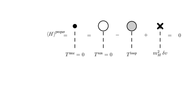
Figure 1: Renormalization condition in the alternative tadpole scheme: With the neutral component $\Phi^{0}$ of the Higgs doublet $\Phi$ defined as $\Phi^{0}=(v+H)/\sqrt{2}$, the requirement for the VEV to represent the true minimum of the Higgs potential translates into $\langle H\rangle^{\text{proper}}=0$ or, equivalently, the renormalized tadpole graph (white blob) to vanish. The proper VEV coincides with the tree-level VEV (fixed by the condition $T^{\text{tree}}=0$). Together with the renormalization condition $T^{\text{ren}}=0$, this relates the tadpole loop diagram (grey blob) at a given loop order to the VEV counterterm.

Since at loop level the proper VEV is given by the renormalized one, and in the FJ scheme coincides with the tree-level VEV, we have

$$\left.v^{\text{ren}}\right|_{\text{FJ}}=v^{\text{tree}}=\left.\frac{2m_{W}}{g}\right|^{\text{tree}}\;.$$ (4.47)

When a given $v$-dependent Lagrangian is used at higher orders these tree-level parameters $\{g,m_{W}\}^{\text{tree}}$ still have to be renormalized, and they are then replaced by their corresponding renormalized parameters as

$$\left.\frac{2m_{W}}{g}\right|^{\text{tree}}\to\left.\frac{2m_{W}}{g}\right|^{\text{ren}}_{\text{FJ}}+\underbrace{\left.\frac{2m_{W}}{g}\left(\frac{\delta m_{W}^{2}}{2m_{W}^{2}}-\frac{\delta g}{g}\right)\right|_{\text{FJ}}}_{\equiv\Delta v}\;.$$ (4.48)

It is important to note that $\Delta v$ is a mere label and not a VEV counterterm as such. This makes obvious that $\delta v$ and $\Delta v$ are completely unrelated. In particular, they feature a totally different divergence structure. Figure 1 depicts the renormalization condition for the alternative tadpole scheme. In the standard scheme, on the other hand, the proper VEV is obtained from the minimisation of the gauge-dependent loop-corrected potential and hence is in principle gauge dependent. An equivalent condition to the FJ scheme requires the renormalized tadpole to vanish. Together with the requirement of the tree-level tadpole to be zero, this fixes the tadpole counterterm, which features here explicitly, as the tadpole is an input parameter in the standard scheme, cf. Fig. 2.

Figure 2: Renormalization condition in the standard tadpole scheme: The requirement of the renormalized tadpole graph (white blob) to vanish together with the tree-level tadpole being zero fixes the tadpole counterterm.

For the singlet VEV $v_{S}$ a similar distinction, i.e. $\delta v_{S}$ versus $\Delta v_{S}$ has to be made. When $v_{S}$ is related to measurable parameters the NLO VEV shift $\Delta v_{s}$ denotes the corresponding combination of parameter counterterms, similarly to  Eq. (4.48). In Ref. [47] it was shown that, in an $R_{\xi}$ gauge, a divergent part for $\Delta v_{S}$ in the standard scheme is precluded at one loop if the scalar field obeys a rigid invariance. This is the case for typical singlet-extended Higgs sectors, e.g. the real singlet model [42], and thereby the N2HDM singlet scalar. In all these cases the singlet field is disconnected from the gauge sector and hence invariant under global gauge transformations. The conclusion of Ref. [47] relies on the use of the standard scheme, where the renormalized VEV coincides with the loop-corrected one as the renormalized tadpoles are set to zero. However, this no longer applies if the VEVs are renormalized in the alternative tadpole scheme. In this case $\Delta v^{\text{FJ}}_{S}$ becomes indeed a UV-divergent quantity. We can prove it to cancel part of the UV poles that genuinely appear if one-loop amplitudes are computed in the FJ-scheme, when the corresponding tree-level amplitudes are directly sensitive to the singlet VEV $v_{S}$. Salient examples are the Higgs-to-Higgs decays, which we discuss in detail in Section 6.

4.1 Alternative tadpole scheme for the N2HDM

In the following, we elaborate in detail the implications of the alternative tadpole scheme. We derive the necessary relations for the N2HDM, highlighting the differences with respect to the 2HDM case, derived in [36]. At tree level the minimum conditions of the N2HDM potential lead to the three relations Eqs. (2.12)-(2.14) for the tadpole parameters, or alternatively

$$T_{1}^{\text{tree}}=0\;,\quad T_{2}^{\text{tree}}=0\quad\mbox{and}\quad T_{3}^{\text{tree}}=0\;.$$ (4.50)

These can be used to replace the parameters $m_{11}^{2}$, $m_{22}^{2}$ and $m_{S}^{2}$ by the VEVs $v_{1}$, $v_{2}$ and $v_{S}$. Note, however, that at arbitrary loop order, this may only be done after the proper VEVs are taken into account in the Higgs potential. More precisely, at NLO the VEVs are modified in order to take into account the NLO effects, as

$$v_{i}^{\text{bare}}=v_{i}^{\text{ren}}+\delta v_{i}\stackrel{{\scriptstyle\text{FJ}}}{{=}}v_{i}^{\text{tree}}+\delta v_{i}\,,\quad i=1,2,S\;.$$ (4.51)

In the alternative tadpole scheme, $\delta v_{1}$, $\delta v_{2}$ and $\delta v_{S}$ correspond to the proper doublet and singlet VEV counterterms in the gauge basis. In turn, $v_{i}^{\text{ren}}$ are the proper VEVs, i.e. in the FJ scheme the renormalized VEVs (coinciding with the tree-level VEVs), and hence the VEVs that generate the necessary mass relations for the gauge bosons, fermions and the scalars. The VEVs are called the proper VEVs if the gauge-invariant relations presented in Fig. 1 (for the SM case) are fulfilled at all orders, which means that the VEVs represent the true vacuum state of the theory at all orders in perturbation theory. At NLO, we insert the relations Eq. (4.51) into the tadpole relations Eqs. (2.12)-(2.14). At NLO, the left-hand side of the equations is given by

$$T_{i}^{\text{bare}}=\underbrace{T_{i}^{\text{tree}}}_{=0}+T_{i}^{\text{loop}}=T_{i}^{\text{loop}}\;,\quad i\equiv 1,2,3\;.$$ (4.52)

We then get the NLO expressions for Eqs. (2.12)-(2.14),

$$T_{1}^{\text{loop}} = T_{1}^{\text{tree}}+\bigg{(}m_{12}^{2}\frac{v_{2}^{\text{tree}}}{v_{1}^{\text{tree}}}+\lambda_{1}(v_{1}^{\text{tree}})^{2}\bigg{)}\delta v_{1}+\bigg{(}-m_{12}^{2}+\lambda_{345}v_{1}^{\text{tree}}v_{2}^{\text{tree}}\bigg{)}\delta v_{2}+\lambda_{7}v_{1}^{\text{tree}}v_{S}^{\text{tree}}\,\delta v_{S}$$

$$T_{2}^{\text{loop}} = T_{2}^{\text{tree}}+\bigg{(}-m_{12}^{2}+\lambda_{345}v_{1}^{\text{tree}}v_{2}^{\text{tree}}\bigg{)}\delta v_{1}+\bigg{(}m_{12}^{2}\frac{v_{1}^{\text{tree}}}{v_{2}^{\text{tree}}}+\lambda_{2}(v_{2}^{\text{tree}})^{2}\bigg{)}\delta v_{2}+\lambda_{8}v_{2}^{\text{tree}}v_{S}^{\text{tree}}\,\delta v_{S}$$

(4.54)

$$T_{3}^{\text{loop}} = T_{3}^{\text{tree}}+\lambda_{6}(v_{S}^{\text{tree}})^{2}\delta v_{S}+\lambda_{7}v_{1}^{\text{tree}}v_{S}^{\text{tree}}\delta v_{1}+\lambda_{8}v_{2}^{\text{tree}}v_{S}^{\text{tree}}\delta v_{2}~{}.$$ (4.55)

Since the NLO effects for the VEVs have been taken into account in form of the counterterms in Eq. (4.51), the FJ-renormalized VEVs $v_{i}^{\text{tree}}=v_{i}^{\text{ren}}$ now represent the true ground states of the theory, namely those for which $\langle\rho_{i}\rangle=0$. The tree-level relations in Eq. (4.50) can therefore be applied, and, in so doing, the VEV counterterms $\delta v_{1},$ $\delta v_{2}$ and $\delta v_{S}$ are given in terms of the tadpole loops $T_{1}^{\text{loop}}$, $T_{2}^{\text{loop}}$ and $T_{3}^{\text{loop}}$. By comparing with the squared mass matrix $M_{\rho}^{2}$ of Eq. (2.23) we find analytically

$$\left(\begin{array}[]{c}T_{1}^{\text{loop}}\\ T_{2}^{\text{loop}}\\ T_{3}^{\text{loop}}\end{array}\right) = \left(\begin{array}[]{ccc}m_{12}^{2}t_{\beta}+\lambda_{1}\,(v^{\text{tree}})^{2}\,c_{\beta}^{2}&-m_{12}^{2}+\lambda_{345}\,(v^{\text{tree}})^{2}\,s_{\beta}c_{\beta}&\lambda_{7}c_{\beta}\,v^{\text{tree}}\,v^{\text{tree}}_{S}\\ -m_{12}^{2}+\lambda_{345}\,(v^{\text{tree}})^{2}\,s_{\beta}c_{\beta}&m_{12}^{2}/t_{\beta}+\lambda_{2}\,(v^{\text{tree}})^{2}\,s_{\beta}^{2}&\lambda_{8}s_{\beta}\,v^{\text{tree}}\,v^{\text{tree}}_{S}\\ \lambda_{7}c_{\beta}\,v^{\text{tree}}\,v^{\text{tree}}_{S}&\lambda_{8}s_{\beta}\,v^{\text{tree}}\,v^{\text{tree}}_{S}&\lambda_{6}\,(v^{\text{tree}}_{S})^{2}\end{array}\right)\left(\begin{array}[]{c}\delta v_{1}\\ \delta v_{2}\\ \delta v_{S}\end{array}\right)$$ (4.65)

$$= \mathcal{M}^{2}_{\rho}\Big{\lvert}_{T_{i}=0}\,\left(\begin{array}[]{c}\delta v_{1}\\ \delta v_{2}\\ \delta v_{S}\end{array}\right)\,.$$ (4.69)

Rotation to the mass basis yields

$$\left(\begin{array}[]{c}\delta v_{H_{1}}\\ \delta v_{H_{2}}\\ \delta v_{H_{3}}\end{array}\right)\,=\left(\begin{array}[]{c}\frac{T_{H_{1}}^{\text{loop}}}{m^{2}_{H_{1}}}\\ \frac{T_{H_{2}}^{\text{loop}}}{m^{2}_{H_{2}}}\\ \frac{T_{H_{3}}^{\text{loop}}}{m^{2}_{H_{3}}}\end{array}\right)\;,$$ (4.70)

where $T_{H_{i}}^{\text{loop}}=R(\alpha_{i})T_{i}^{\text{loop}}$, and hence

$$\left(\begin{array}[]{c}\delta v_{1}\\ \delta v_{2}\\ \delta v_{S}\end{array}\right)=R(\alpha_{i})^{T}\,\left(\begin{array}[]{c}\frac{T_{H_{1}}^{\text{loop}}}{m^{2}_{H_{1}}}\\ \frac{T_{H_{2}}^{\text{loop}}}{m^{2}_{H_{2}}}\\ \frac{T_{H_{3}}^{\text{loop}}}{m^{2}_{H_{3}}}\end{array}\right)\,.$$ (4.71)

The latter identity is helpful in practice, as the calculation of the tadpole diagrams is usually performed in the mass basis, but the VEV shifts are introduced most conveniently in the gauge basis. Rewriting Eq. (4.70), the quantities $\delta v_{H_{i}}$ can be interpreted as connected tadpole diagrams, containing the Higgs tadpole and its propagator at zero momentum transfer,

$$\delta v_{H_{i}}=\frac{-i}{m_{H_{i}}^{2}}iT_{H_{i}}^{\text{loop}}=\frac{-i}{m_{H_{i}}^{2}}~{}\mathord{\left(\rule{0.0pt}{30.11249pt}\right.\vbox{ \hbox{ \includegraphics[height=57.21375pt,trim=51.21495pt 34.1433pt 48.36967pt 28.45274pt,clip]{TadpoleDiagramHiggsBasis.pdf} } }\left.\rule{0.0pt}{30.11249pt}\right)=\left(\rule{0.0pt}{30.11249pt}\right.\vbox{ \hbox{ \includegraphics[height=57.21375pt,trim=49.79231pt 34.1433pt 41.54103pt 28.45274pt,clip]{TadpoleDiagramHiggsBasisWithVertex.pdf} } }\left.\rule{0.0pt}{30.11249pt}\right)}~{}.$$ (4.72)

We want to emphasize again that in the alternative tadpole scheme Eq. (4.72) defines the counterterms of the vacuum expectation values. In contrast to the standard scheme, no tadpole counterterms are introduced. Tadpole graphs appear through the gauge-invariant condition in Fig. 1.

Once the leading-order VEVs are promoted to higher orders, namely by inserting Eq. (4.51) into a generic VEV-dependent Lagrangian ${\cal L}(v_{1},v_{2},v_{S})$, the contribution of the VEV counterterms $\delta v_{1}$, $\delta v_{2}$ and $\delta v_{S}$, as given by Eq. (4.71), is equivalent to introducing explicit tadpole graphs in all loop amplitudes. Moreover, all tree-level relations between the VEVs and the weak sector parameters (masses, coupling constants) hold again. In particular, for the doublet VEVs this means with ($v_{1}^{2}+v_{2}^{2}=v^{2}$)

$$\left.v^{\text{ren}}\right|_{\text{FJ}}=v^{\text{tree}}=\cfrac{2m_{W}}{g}\Big{\lvert}^{\text{tree}}\,$$ (4.73)

then

$$\left.v_{1}^{\text{ren}}\right|_{\text{FJ}}=v_{1}^{\text{tree}}=\cfrac{2m_{W}c_{\beta}}{g}\Big{\lvert}^{\text{tree}}\qquad\mbox{and}\qquad\left.v_{2}^{\text{ren}}\right|_{\text{FJ}}=v_{2}^{\text{tree}}=\cfrac{2m_{W}s_{\beta}}{g}\Big{\lvert}^{\text{tree}}\;.$$ (4.74)

By applying the renormalization conditions for the VEVs, the tree-level VEVs ensure the true ground state of the potential. Since they are not directly related to a physical observable, we express the FJ-renormalized doublet VEVs in terms of physical tree-level parameters, here $m_{W}$, $g$ and the mixing angle $\beta$. In higher order calculations, these parameters are then renormalized by choosing physical renormalization conditions. To better illustrate the implications of the alternative tadpole scheme, we consider the scalar-vector-vector vertex between the physical $H_{1}$ and a $W$ boson pair. We first define the Feynman rules, needed in the following, by

$$H_{1}W^{\mu}W^{\nu} : ig_{H_{1}WW}\,g^{\mu\nu}$$ (4.75)

$$H_{1}H_{j}W^{\mu}W^{\nu} : ig_{H_{1}H_{j}WW}\,g^{\mu\nu}\>,\quad j=1,2,3\;.$$ (4.76)

The coupling constants for the triple vertex in terms of the mixing angles and the VEVs $v_{1}$ and $v_{2}$ are

$$g_{H_{1}WW} \equiv g_{HWW}^{\text{SM}}\,\kappa_{H_{1}WW}$$ (4.77)

$$= gm_{W}c_{\alpha_{2}}c_{\beta-\alpha_{1}}=\frac{g^{2}vc_{\alpha_{2}}c_{\beta-\alpha_{1}}}{2}=\frac{g^{2}c_{\alpha_{2}}}{2}(c_{\alpha_{1}}v_{1}+s_{\alpha_{1}}v_{2})\;,$$

and for the quartic vertices

$$g_{H_{1}H_{1}WW} \equiv \kappa_{H_{1}H_{1}ZZ}\,g_{HWW}^{\text{SM}}=\frac{g^{2}\,c_{\alpha_{2}}^{2}}{2}$$

$$g_{H_{1}H_{2}WW} \equiv \kappa_{H_{1}H_{2}ZZ}\,g_{HWW}^{\text{SM}}=-\frac{g^{2}\,c_{\alpha_{2}}s_{\alpha_{2}}s_{\alpha_{3}}}{2}$$

$$g_{H_{1}H_{3}WW} \equiv \kappa_{H_{1}H_{3}ZZ}\,g_{HWW}^{\text{SM}}=-\frac{g^{2}\,c_{\alpha_{2}}s_{\alpha_{2}}c_{\alpha_{3}}}{2}\;.$$ (4.78)

When expressing the couplings in terms of the VEVs, care has to be taken to differentiate between the angle $\beta$ in the sense of a mixing angle and $\beta$ in the sense of the ratio of the VEVs. Only the latter is to be replaced by the VEVs that are to be renormalized. The same distinction must be applied for the $\alpha_{i}$. Note that in all couplings but the trilinear and quartic Higgs self-couplings the angles $\alpha_{i}$ have the roles of mixing angles. Only in the Higgs self-couplings, the $\alpha_{i}$ partly appear in the sense of the ratio of N2HDM potential parameters. Bearing these considerations in mind, we see that the quartic couplings do not receive any $\delta v_{i}$, whereas $g_{H_{1}WW}$ contains $\beta$ as ratio of the VEVs. Instead, the angles $\alpha_{1}$ and $\alpha_{2}$ are mixing angles here. At NLO, we therefore have to make the replacement

$$\begin{split}ig_{H_{1}WW}~{}&=~{}\frac{ig^{2}c_{\alpha_{2}}}{2}(c_{\alpha_{1}}v_{1}^{\text{tree}}+s_{\alpha_{1}}v_{2}^{\text{tree}})+\frac{ig^{2}c_{\alpha_{2}}}{2}(c_{\alpha_{1}}\delta v_{1}+s_{\alpha_{1}}\delta v_{2})\\ &\stackrel{{\scriptstyle(\ref{eq:vevshift-tadpole-mass})}}{{=}}ig_{H_{1}WW}+\frac{ig^{2}c_{\alpha_{2}}}{2}\left[c_{\alpha_{2}}\,\cfrac{T_{H_{1}}^{\text{loop}}}{m^{2}_{H_{1}}}-s_{\alpha_{2}}s_{\alpha_{3}}\,\cfrac{T_{H_{2}}^{\text{loop}}}{m^{2}_{H_{2}}}-s_{\alpha_{2}}c_{\alpha_{3}}\,\cfrac{T_{H_{3}}^{\text{loop}}}{m^{2}_{H_{3}}}\right]\\ &=ig_{H_{1}WW}\\ &+ig_{H_{1}H_{1}WW}\,\left(\frac{-i}{m_{H_{1}}^{2}}\right)\,iT_{H_{1}}^{\text{loop}}+ig_{H_{1}H_{2}WW}\,\left(\frac{-i}{m_{H_{2}}^{2}}\right)\,iT_{H_{2}}^{\text{loop}}+ig_{H_{1}H_{3}WW}\,\left(\frac{-i}{m_{H_{3}}^{2}}\right)\,iT_{H_{3}}^{\text{loop}}\\ &=ig_{H_{1}WW}+\mathord{\left(\rule{0.0pt}{40.15pt}\right.\vbox{ \hbox{ \includegraphics[height=80.29999pt,clip]{VEVShiftResultVertexH1.pdf} } }+\vbox{ \hbox{ \includegraphics[height=80.29999pt,clip]{VEVShiftResultVertexH2.pdf} } }+\vbox{ \hbox{ \includegraphics[height=80.29999pt,clip]{VEVShiftResultVertexH3.pdf} } }\left.\rule{0.0pt}{40.15pt}\right)_{\textrm{trunc}}}\\ &\equiv ig_{H_{1}WW}^{\textrm{tad}}\;.\end{split}$$ (4.79)

The subscript ’trunc’ means that all Lorentz structure of the vector bosons as well as the Lorentz structure of the coupling has been suppressed here for simplicity. The second term in the second line generates, through the VEV counterterms $\delta v_{i}$, the tadpole diagrams contributing to the scalar-vector-vector vertex. On the other hand, as the VEVs in this expression have already been expanded to NLO through $v_{i}\to v_{i}^{\text{tree}}+\delta v_{i}$, we use all tree-level relations, in particular Eq. (4.74), to fix the (FJ-renormalized) VEVs $v_{i}^{\text{tree}}$ in terms of the tree-level weak sector parameters and the angle $\beta$. At loop level the EW parameters and mixing angles that enter the coupling, here $g$, $m_{W}$, $\beta$, $\alpha_{1}$ and $\alpha_{2}$ have to be renormalized, i.e. we replace them by their renormalized values plus the corresponding counterterms, cf. Eq. (3.1). We then get for the vertex of Eq. (4.79)

$$ig_{H_{1}WW}^{\text{tad}}+igm_{W}c_{\alpha_{2}}c_{\beta-\alpha_{1}}\left[\frac{\delta g}{g}+\frac{\delta m_{W}^{2}}{2m_{W}^{2}}-t_{\alpha_{2}}\delta\alpha_{2}-t_{\beta-\alpha_{1}}(\delta\beta-\delta\alpha_{1})\right]\;.$$ (4.80)

The exact form of these counterterms depends on the renormalization conditions, which will be given in the next section.

Our derivation also shows the difference with respect to the 2HDM, namely the last two terms in Eq. (4.79) do not arise in the 2HDM. They are due to the additional singlet-doublet mixing and have no counterpart in a pure 2HDM structure (cf. Eq. (A.61) of [36]).

As a final remark, let us summarise the key differences with respect to the standard tadpole scheme. In the latter case, VEV counterterms of the form of Eq. (4.72) are strictly speaking not introduced. Instead, one introduces renormalized tadpoles and tadpole counterterms, fulfilling the same condition as in Fig. 1 - that is, $T_{i}^{\text{ren}}=0$ with $T_{i}^{\text{ren}}=T_{i}^{\text{loop}}-\delta T_{i}$. In doing so, the VEVs correspond to the ground state of the loop-corrected scalar potential, and the corresponding VEV relations to weak sector parameters hold order-by-order. Due to the fact that in the standard tadpole scheme one considers the VEVs from the one-loop corrected potential (in contrast to the alternative scheme, where one considers the tree-level VEVs), VEV diagrams in the self-energies and vertices explicitly vanish and thus need not be taken into account, at the expense of defining mass counterterms which become manifestly gauge dependent.

In practice, the rigorous introduction of the VEV counterterms in the alternative tadpole scheme yields the following rules for its application in the renormalization of a generic process within the N2HDM:

Figure 3: Modified self-energy $i\Sigma^{\textrm{tad}}(p^{2})$ in the alternative tadpole scheme, consisting of all 1 particle-irreducible (PI) self-energy diagrams together with the one-loop tadpole diagrams, indicated by a gray blob.

1. Include explicit tadpole contributions in all self-energies used to define the (off-diagonal) wave function renormalization constants and wherever the self-energies appear in the counterterms, such that now $\Sigma^{\text{tad}}(p^{2})$ contains the additional tadpole contributions, cf. Fig. 3.

2. Include explicit tadpole contributions in the virtual vertex corrections, if the tadpole insertions are connected to an existing coupling. This is applicable e.g. to all triple Higgs self-interactions as well as to the Higgs couplings to gauge bosons.

In the alternative tadpole scheme not only the angular counterterms but also the mass counterterms become gauge independent. This has been shown for the electroweak sector in [48]. All counterterms of the electroweak sector have exactly the same structure as in the standard scheme. Only the self-energies $\Sigma$ have to be replaced by the self-energies $\Sigma^{\text{tad}}$ containing the tadpole contributions. Note however, that there are no tadpole contributions to the transverse photon-$Z$ self-energy $\Sigma_{\gamma Z}^{T}$ nor to the transverse photon self-energy $\Sigma_{\gamma\gamma}^{T}$ so that

$$\Sigma_{\gamma Z/\gamma\gamma}^{\text{tad},T}=\Sigma_{\gamma Z/\gamma\gamma}^{T}\;.$$ (4.81)

Having introduced the tadpole scheme, we now list explicitly the counterterms needed in the computation of the electroweak corrections. In particular, we illustrate the renormalization of the N2HDM Higgs sector.

5 Renormalization conditions

With the previous section we are now able to specify the counterterms needed in the renormalization of the N2HDM. Those of the EW and Yukawa sector correspond to the ones of the SM, while differences obviously arise in the Higgs sector itself. For completeness, all counterterms of the model will be listed, although not all of them will be necessary to study the sample processes discussed in Section 7.

5.1 Counterterms of the gauge sector

The gauge bosons are renormalized through OS conditions implying the mass counterterms

$$\delta m_{W}^{2}=\mbox{Re}\Sigma^{\text{tad},T}_{WW}(m_{W}^{2})\quad\mbox{and}\quad\delta m_{Z}^{2}=\mbox{Re}\Sigma^{\text{tad},T}_{ZZ}(m_{Z}^{2})\;,$$ (5.82)

where $T$ denotes the transverse part of the self-energy including the tadpole contributions. The wave function renormalization constants that guarantee the correct OS properties are given by

$$\delta Z_{WW} = -\mbox{Re}\left.\frac{\partial\Sigma^{T}_{WW}(p^{2})}{\partial p^{2}}\right|_{p^{2}=m_{W}^{2}}$$ (5.83)

$$\left(\begin{array}[]{cc}\delta Z_{ZZ}&\delta Z_{Z\gamma}\\ \delta Z_{\gamma Z}&\delta Z_{\gamma\gamma}\end{array}\right) = \left(\begin{array}[]{cc}-\mbox{Re}\left.\frac{\partial\Sigma^{T}_{ZZ}(p^{2})}{\partial p^{2}}\right|_{p^{2}=m_{Z}^{2}}&2\frac{\Sigma^{T}_{Z\gamma}(0)}{m_{Z}^{2}}\\ -2\mbox{Re}\frac{\Sigma^{T}_{Z\gamma}(m_{Z}^{2})}{m_{Z}^{2}}&-\left.\frac{\partial\Sigma^{T}_{\gamma\gamma}(p^{2})}{\partial p^{2}}\right|_{p^{2}=0}\end{array}\right)\;.$$ (5.88)

Note that in Eqs. (5.83) and (5.88) they are the same in the standard and in the alternative tadpole scheme introduced above. The reason is that the tadpoles are independent of the external momentum so that the derivatives of the self-energies do not change. Furthermore, $\Sigma_{\gamma Z}^{T}$ is identical in both schemes, as alluded to above. For better readability we therefore drop the superscript ’tad’ here and wherever possible. For the same reasons the counterterm for the electric charge is invariant with respect to the choice of the tadpole scheme. The electric charge is renormalized to be the full electron-positron photon coupling for OS external particles in the Thomson limit. This implies that all corrections to this vertex vanish OS and for zero momentum transfer. The counterterm for the electric charge in terms of the transverse photon-photon and photon-Z self-energies reads [49]

$$\delta Z_{e}^{\alpha(0)} = \frac{1}{2}\left.\frac{\partial\Sigma^{T}_{\gamma\gamma}(k^{2})}{\partial k^{2}}\right|_{k^{2}=0}+\frac{s_{W}}{c_{W}}\frac{\Sigma_{\gamma Z}^{T}(0)}{m_{Z}^{2}}\;.$$ (5.89)

The sign in the second term of Eq. (5.89) differs from the one in [49] because we have adopted different sign conventions in the covariant derivative of Eq. (2.2). In our computation we will use the fine structure constant at the $Z$ boson mass $\alpha(m_{Z}^{2})$ as input. This way the results are independent of large logarithms due to light fermions $f\neq t$. The counterterm $\delta Z_{e}$ is therefore modified as [49]

$$\delta Z_{e}^{\alpha(m_{Z}^{2})} = \delta Z_{e}^{\alpha(0)}-\frac{1}{2}\Delta\alpha(m_{Z}^{2})$$ (5.90)

$$\Delta\alpha(m_{Z}^{2}) = \left.\frac{\partial\Sigma^{T}_{\gamma\gamma}(k^{2})}{\partial k^{2}}\right|_{k^{2}=0}-\frac{\Sigma^{T}_{\gamma\gamma}(m_{Z}^{2})}{m_{Z}^{2}}\;,$$ (5.91)

where the transverse part of the photon self-energy $\Sigma^{T}_{\gamma\gamma}$ in Eq. (5.91) includes only the light fermion contributions. The calculation of the EW one-loop corrected Higgs decay widths also requires the renormalization of the weak coupling $g$, which can be related to $e$ and the gauge boson masses as

$$g = \frac{em_{Z}}{\sqrt{m_{Z}^{2}-m_{W}^{2}}}\;.$$ (5.92)

Its counterterm can therefore be expressed in terms of the electric charge and gauge boson mass counterterms through

$$\frac{\delta g}{g}=\delta Z_{e}-\frac{1}{2(1-m_{Z}^{2}/m_{W}^{2})}\left(\frac{\delta m_{W}^{2}}{m_{W}^{2}}-\frac{\delta m_{Z}^{2}}{m_{Z}^{2}}\right)\;.$$ (5.93)

5.2 Counterterms of the fermion sector

Defining the following structure for the fermion self-energies

$$\Sigma_{f}(p^{2})=/{\!\!\!p}\Sigma^{L}_{f}(p^{2})P_{L}+/{\!\!\!p}\Sigma^{R}_{f}(p^{2})P_{R}+m_{f}\Sigma^{Ls}_{f}(p^{2})P_{L}+m_{f}\Sigma^{Rs}_{f}(p^{2})P_{R}$$ (5.94)

the fermion mass counterterms applying OS conditions are given by

$$\frac{\delta m_{f}}{m_{f}}=\frac{1}{2}\mbox{Re}\left[\Sigma^{\text{tad},L}_{f}(m_{f}^{2})+\Sigma^{\text{tad},R}_{f}(m_{f}^{2})+\Sigma^{\text{tad},Ls}_{f}(m_{f}^{2})+\Sigma^{\text{tad},Rs}_{f}(m_{f}^{2})\right]\;.$$ (5.95)

The fermion wave function renormalization constants are determined from

$$\delta Z^{L/R}_{f} = -\mbox{Re}\Sigma^{\text{tad},L/R}_{f}(m_{f}^{2})$$

$$-m_{f}^{2}\frac{\partial}{\partial p^{2}}\mbox{Re}\left.\left(\Sigma^{L/R}_{f}(p^{2})+\Sigma^{R/L}_{f}(p^{2})+\Sigma^{L/Rs}_{f}(p^{2})+\Sigma^{R/Ls}_{f}(p^{2})\right)\right|_{p^{2}=m_{f}^{2}}\,.$$

5.3 Higgs field and mass counterterms

The OS conditions for the physical Higgs bosons yield the mass counterterms ($i=1,2,3$)

$$\delta m_{H_{i}}^{2} = \mbox{Re}[\Sigma^{\text{tad}}_{H_{i}H_{i}}(m_{H_{i}}^{2})]$$ (5.97)

$$\delta m_{A}^{2} = \mbox{Re}[\Sigma^{\text{tad}}_{AA}(m_{A}^{2})]$$ (5.98)

$$\delta m_{H^{\pm}}^{2} = \mbox{Re}[\Sigma^{\text{tad}}_{H^{\pm}H^{\pm}}(m_{H^{\pm}}^{2})]\;.$$ (5.99)

Having absorbed the tadpoles into the self-energies, no tadpole counterterms appear explicitly in the mass counterterms any more, in contrast to the corresponding expressions in the standard tadpole scheme. The OS conditions for the Higgs bosons yield the following wave function renormalization counterterm $3\times 3$ matrix for the CP-even neutral N2HDM scalars,

$$\delta Z_{H_{i}H_{j}}=\left(\begin{array}[]{ccc}-\mbox{Re}\left.\frac{\partial\Sigma_{H_{1}H_{1}}(k^{2})}{\partial k^{2}}\right|_{k^{2}=m_{H_{1}}^{2}}&2\frac{\mbox{Re}\left[\Sigma^{\text{tad}}_{H_{1}H_{2}}(m_{H_{2}}^{2})\right]}{m_{H_{1}}^{2}-m_{H_{2}}^{2}}&2\frac{\mbox{Re}\left[\Sigma^{\text{tad}}_{H_{1}H_{3}}(m_{H_{3}}^{2})\right]}{m_{H_{1}}^{2}-m_{H_{3}}^{2}}\\[8.5359pt] 2\frac{\mbox{Re}\left[\Sigma^{\text{tad}}_{H_{2}H_{1}}(m_{H_{1}}^{2})\right]}{m_{H_{2}}^{2}-m_{H_{1}}^{2}}&-\mbox{Re}\left.\frac{\partial\Sigma_{H_{2}H_{2}}(k^{2})}{\partial k^{2}}\right|_{k^{2}=m_{H_{2}}^{2}}&2\frac{\mbox{Re}\left[\Sigma^{\text{tad}}_{H_{2}H_{3}}(m_{H_{3}}^{2})\right]}{m_{H_{2}}^{2}-m_{H_{3}}^{2}}\\ 2\frac{\mbox{Re}\left[\Sigma^{\text{tad}}_{H_{3}H_{1}}(m_{H_{1}}^{2})\right]}{m_{H_{3}}^{2}-m_{H_{1}}^{2}}&2\frac{\mbox{Re}\left[\Sigma^{\text{tad}}_{H_{3}H_{2}}(m_{H_{2}}^{2})\right]}{m_{H_{3}}^{2}-m_{H_{2}}^{2}}&-\mbox{Re}\left.\frac{\partial\Sigma_{H_{3}H_{3}}(k^{2})}{\partial k^{2}}\right|_{k^{2}=m_{H_{3}}^{2}}\end{array}\right)$$ (5.102)

And in the CP-odd and charged sector we have the $2\times 2$ matrices

$$\left(\begin{array}[]{cc}\delta Z_{G^{0}G^{0}}&\delta Z_{G^{0}A}\\ \delta Z_{AG^{0}}&\delta Z_{AA}\end{array}\right) = \left(\begin{array}[]{cc}-\mbox{Re}\left.\frac{\partial\Sigma_{G^{0}G^{0}}(k^{2})}{\partial k^{2}}\right|_{k^{2}=0}&-2\frac{\mbox{Re}\left[\Sigma^{\text{tad}}_{G^{0}A}(m_{A}^{2})\right]}{m_{A}^{2}}\\[8.5359pt] 2\frac{\mbox{Re}\left[\Sigma^{\text{tad}}_{G^{0}A}(0)\right]}{m_{A}^{2}}&-\mbox{Re}\left.\frac{\partial\Sigma_{AA}(k^{2})}{\partial k^{2}}\right|_{k^{2}=m_{A}^{2}}\end{array}\right)$$ (5.108)

$$\left(\begin{array}[]{cc}\delta Z_{G^{\pm}G^{\pm}}&\delta Z_{G^{\pm}H^{\pm}}\\ \delta Z_{H^{\pm}G^{\pm}}&\delta Z_{H^{\pm}H^{\pm}}\end{array}\right) = \left(\begin{array}[]{cc}-\mbox{Re}\left.\frac{\partial\Sigma_{G^{\pm}G^{\pm}}(k^{2})}{\partial k^{2}}\right|_{k^{2}=0}&-2\frac{\mbox{Re}\left[\Sigma^{\text{tad}}_{G^{\pm}H^{\pm}}(m_{H^{\pm}}^{2})\right]}{m_{H^{\pm}}^{2}}\\[8.5359pt] 2\frac{\mbox{Re}\left[\Sigma^{\text{tad}}_{G^{\pm}H^{\pm}}(0)\right]}{m_{H^{\pm}}^{2}}&-\mbox{Re}\left.\frac{\partial\Sigma_{H^{\pm}H^{\pm}}(k^{2})}{\partial k^{2}}\right|_{k^{2}=m_{H^{\pm}}^{2}}\end{array}\right)$$ (5.113)

5.4 Angular counterterms

As in the 2HDM, we renormalize the mixing angles based on the definition of the counterterms through off-diagonal wave function renormalization constants and combine this with the alternative tadpole approach together with the application of the pinch technique in order to arrive at an unambiguous gauge-independent definition of the mixing angle counterterms. Let us note that a process-dependent renormalization of the mixing angles would also lead to a gauge-independent renormalization, as shown in [36] for the 2HDM case. In the N2HDM the situation becomes more involved as four different processes need to be identified to fix all mixing angle counterterms $\delta\alpha_{i}$ and $\delta\beta$. Moreover, the construction of such a process-dependent scheme is complicated by the fact that the different Higgs decay modes typically rely on more than one mixing angle, implying that the different angular counterterms appear as linear combinations in each individual vertex counterterm. It is therefore imperative to choose a set of processes where the angular counterterm dependences enter as a linearly independent combination, such that they can be fixed unambiguously through linear combinations of the different decay widths. Moreover, all these processes have to be phenomenologically accessible. The process-dependent renormalization of the N2HDM mixing angles is hence rather unpractical from a physical point of view, and we will therefore not consider it any further.

While the expression for the counterterm in the charged and CP-odd sector, $\delta\beta$, in terms of the off-diagonal wave function renormalization constants does not change with respect to the 2HDM, this is not the case for the mixing angle counterterms $\delta\alpha_{i}$ in the CP-even sector. We therefore present their derivation here. It is based on the idea of making the counterterms $\delta\alpha_{i}$ (and also $\delta\beta$) appear in the inverse propagator matrix and thereby in the wave function renormalization constants in a way that is consistent with the internal relations of the N2HDM. This can be achieved by performing the renormalization in the physical basis $(H_{1},H_{2},H_{3})$, but temporarily switching to the gauge basis $(\rho_{1},\rho_{2},\rho_{3})$, and back again. For the CP-even sector of the N2HDM this means,

$$\left(\begin{array}[]{c}H_{1}\\ H_{2}\\ H_{3}\end{array}\right)_{\text{bare}} = R(\alpha_{i})\,\Bigg{\lvert}_{\text{bare}}\left(\begin{array}[]{c}\rho_{1}\\ \rho_{2}\\ \rho_{3}\end{array}\right)_{\text{bare}}\quad\rightarrow\qquad R(\alpha_{i}+\delta\,\alpha_{i})\,\sqrt{Z_{\rho_{i}}}\,\left(\begin{array}[]{c}\rho_{1}\\ \rho_{2}\\ \rho_{3}\end{array}\right)$$ (5.123)

$$= \underbrace{R(\delta\alpha_{i})\,R(\alpha_{i})\,\sqrt{Z_{\rho_{i}}}\,R(\alpha_{i})^{T}}_{\sqrt{Z_{H_{i}}}}\,R(\alpha_{i})\,\left(\begin{array}[]{c}\rho_{1}\\ \rho_{2}\\ \rho_{3}\end{array}\right)=\sqrt{Z_{H_{i}}}\,\left(\begin{array}[]{c}H_{1}\\ H_{2}\\ H_{3}\end{array}\right)\,.$$ (5.130)

The field renormalization matrix in the mass basis can be parametrised as

$$\sqrt{Z_{H_{i}}} = R(\delta\alpha_{i})\left(\begin{array}[]{ccc}1+\frac{\delta Z_{H_{1}H_{1}}}{2}&\delta C_{12}&\delta C_{13}\\ \delta C_{21}&1+\frac{\delta Z_{H_{2}H_{2}}}{2}&\delta C_{23}\\ \delta C_{31}&\delta C_{32}&1+\frac{\delta Z_{H_{3}H_{3}}}{2}\end{array}\right)=$$ (5.139)

$$\left(\begin{array}[]{ccc}1+\cfrac{\delta Z_{H_{1}H_{1}}}{2}&c_{\alpha_{1}}c_{\alpha_{3}}\delta\alpha_{1}+s_{\alpha_{3}}\delta\alpha_{2}+\delta C_{12}&c_{\alpha_{3}}\delta\alpha_{2}-s_{\alpha_{3}}c_{\alpha_{2}}\delta\alpha_{1}+\delta C_{13}\\ -c_{\alpha_{2}}c_{\alpha_{3}}\delta\alpha_{1}-s_{\alpha_{3}}\delta\alpha_{2}+\delta C_{21}&1+\cfrac{\delta Z_{H_{2}H_{2}}}{2}&\delta\alpha_{3}+s_{\alpha_{2}}\delta\alpha_{1}+\delta C_{23}\\ -c_{\alpha_{3}}\delta\alpha_{2}+s_{\alpha_{3}}c_{\alpha_{2}}\delta\alpha_{1}+\delta C_{31}&-\delta\alpha_{3}-s_{\alpha_{2}}\delta\alpha_{1}+\delta C_{32}&1+\cfrac{\delta Z_{H_{3}H_{3}}}{2}\end{array}\right)$$

By identifying the off-diagonal elements with the off-diagonal wave function renormalization constants $\delta Z_{H_{i}H_{j}}$ ($i\neq j$), the three neutral CP-even angular counterterms are obtained as

$$\delta\alpha_{1} =\cfrac{c_{\alpha_{3}}}{4\,c_{\alpha_{2}}}\,(\delta Z_{H_{1}H_{2}}-\delta Z_{H_{2}H_{1}})-\cfrac{s_{\alpha_{3}}\,}{4\,c_{\alpha_{2}}}\,(\delta Z_{H_{1}H_{3}}-\delta Z_{H_{3}H_{1}})$$

$$\delta\alpha_{2} =\cfrac{c_{\alpha_{3}}}{4}\,(\delta Z_{H_{1}H_{3}}-\delta Z_{H_{3}H_{1}})+\cfrac{s_{\alpha_{3}}\,}{4}\,(\delta Z_{H_{1}H_{2}}-\delta Z_{H_{2}H_{1}})$$ (5.141)

$$\delta\alpha_{3} =\cfrac{1}{4}\,(\delta Z_{H_{2}H_{3}}-\delta Z_{H_{3}H_{2}})+\cfrac{s_{\alpha_{2}}}{4c_{\alpha_{2}}}\,\left[s_{\alpha_{3}}\left(\delta Z_{H_{1}H_{3}}-\delta Z_{H_{3}H_{1}}\right)-c_{\alpha_{3}}\left(\delta Z_{H_{1}H_{2}}-\delta Z_{H_{2}H_{1}}\right)\right]\,,$$

while the auxiliary counterterms $\delta C_{ij}$ do not play a role in the remainder of the discussion.

The definition of the counterterm $\delta\beta$ can be taken over from the 2HDM. It is derived analogously to the $\delta\alpha_{i}$, but from the charged and CP-odd Higgs sectors. In this case, there are altogether four off-diagonal wave function constants, while only three free parameters to be fixed. For details, we refer to Ref. [36]. There we proposed two different possible counterterm choices for $\beta$, one based on the charged and the other on the CP-odd sector. Also here we will apply these two possible choices, given by

$$\delta\beta^{(1)}=\frac{1}{4}(\delta Z_{G^{\pm}H^{\pm}}-\delta Z_{H^{\pm}G^{\pm}})$$ (5.142)

and

$$\delta\beta^{(2)} = \frac{1}{4}(\delta Z_{G^{0}A}-\delta Z_{AG^{0}})\;.$$ (5.143)

All wave function renormalization constants appearing in the counterterms Eqs. (5.141), (5.142) and (5.143) are renormalized in the OS scheme and given by the corresponding entries in the wave function counterterm matrices Eqs. (5.102), (5.108) and (5.113). While the use of the alternative tadpole scheme ensures that the angular counterterms can be expressed in a gauge-independent way, at this stage they still contain a dependence on the gauge-fixing parameter. We therefore combine the virtues of the alternative tadpole scheme with the pinch technique [51, 52, 53, 54, 55, 56, 57, 58]. The pinch technique allows us to extract the truly gauge-independent parts of the angular counterterms.

5.4.1 Gauge-independent pinch technique-based angular counterterm schemes

By the application of the pinch technique it possible to define pinched self-energies $\overline{\Sigma}$ which are truly gauge independent. They are built up by the tadpole self-energies evaluated in the Feynman gauge and extra pinched components $\Sigma^{\text{add}}$, i.e.

$$\overline{\Sigma}(p^{2})=\left.\Sigma^{\text{tad}}(p^{2})\right|_{\xi_{V}=1}+\Sigma^{\text{add}}(p^{2})\;,$$ (5.144)

where $\xi_{V}$ stands for the gauge fixing parameters $\xi_{Z}$, $\xi_{W}$ and $\xi_{\gamma}$ of the $R_{\xi}$ gauge. By $\Sigma^{\text{add}}$ we dub the additional (explicitly $\xi_{V}$-independent) self-energy contributions obtained via the pinch technique. It is important to notice that, in order to apply the pinch technique, it is necessary to explicitly include all tadpole topologies, i.e. to use the alternative tadpole scheme. In App. A we present the basic idea of the pinch technique (see also Refs. [51, 52, 53, 54, 55, 56, 57, 58] for a detailed exposition). We exemplarily show, for the CP-even sector, how to proceed in the derivation of the pinched self-energy. Additionally, we give useful formulae on the gauge dependences of the scalar self-energies and for the application of the pinch technique in the N2HDM.

On-shell tadpole-pinched scheme

The self-energy $\Sigma^{\text{add}}$ in Eq. (5.144) is explicitly independent of the gauge fixing parameter $\xi_{V}$. By replacing the wave function renormalization constants in the counterterms Eqs. (5.141), (5.142) and (5.143) with their OS renormalization definitions given by the corresponding entries in the wave function counterterm matrices Eqs. (5.102), (5.108) and (5.113) we arrive, upon expressing these in terms of the pinched self-energies, at the following expressions for the angular counterterms $\delta\alpha_{i}$,

$$\delta_{\alpha_{1}} =\cfrac{c_{\alpha_{3}}}{2c_{\alpha_{2}}}\,\cfrac{\mbox{Re}\,\left(\left[\Sigma^{\text{tad}}_{H_{1}H_{2}}(m^{2}_{H_{2}})+\Sigma^{\text{tad}}_{H_{2}H_{1}}(m^{2}_{H_{1}})\right]_{\xi_{V}=1}+\Sigma^{\text{add}}_{H_{1}H_{2}}(m^{2}_{H_{2}})+\Sigma^{\text{add}}_{H_{2}H_{1}}(m^{2}_{H_{1}})\right)}{m^{2}_{H_{1}}-m^{2}_{H_{2}}}$$

$$-\cfrac{s_{\alpha_{3}}}{2c_{\alpha_{2}}}\,\cfrac{\mbox{Re}\,\left(\left[\Sigma^{\text{tad}}_{H_{1}H_{3}}(m^{2}_{H_{3}})+\Sigma^{\text{tad}}_{H_{3}H_{1}}(m^{2}_{H_{1}})\right]_{\xi_{V}=1}+\Sigma^{\text{add}}_{H_{1}H_{3}}(m^{2}_{H_{3}})+\Sigma^{\text{add}}_{H_{3}H_{1}}(m^{2}_{H_{1}})\right)}{m^{2}_{H_{1}}-m^{2}_{H_{3}}}$$

$$\delta_{\alpha_{2}} =\cfrac{c_{\alpha_{3}}}{2}\,\cfrac{\mbox{Re}\,\left(\left[\Sigma^{\text{tad}}_{H_{1}H_{3}}(m^{2}_{H_{3}})+\Sigma^{\text{tad}}_{H_{3}H_{1}}(m^{2}_{H_{1}})\right]_{\xi_{V}=1}+\Sigma^{\text{add}}_{H_{1}H_{3}}(m^{2}_{H_{3}})+\Sigma^{\text{add}}_{H_{3}H_{1}}(m^{2}_{H_{1}})\right)}{m^{2}_{H_{1}}-m^{2}_{H_{3}}}$$

$$+\cfrac{s_{\alpha_{3}}}{2}\,\cfrac{\mbox{Re}\,\left(\left[\Sigma^{\text{tad}}_{H_{1}H_{2}}(m^{2}_{H_{2}})+\Sigma^{\text{tad}}_{H_{2}H_{1}}(m^{2}_{H_{1}})\right]_{\xi_{V}=1}+\Sigma^{\text{add}}_{H_{1}H_{2}}(m^{2}_{H_{2}})+\Sigma^{\text{add}}_{H_{2}H_{1}}(m^{2}_{H_{1}})\right)}{m^{2}_{H_{1}}-m^{2}_{H_{2}}}$$

$$\delta_{\alpha_{3}} =\cfrac{1}{2}\,\cfrac{\mbox{Re}\,\left[\Sigma^{\text{tad}}_{H_{2}H_{3}}(m^{2}_{H_{3}})+\Sigma^{\text{tad}}_{H_{3}H_{2}}(m^{2}_{H_{2}})\right]_{\xi_{V}=1}+\Sigma^{\text{add}}_{H_{2}H_{3}}(m^{2}_{H_{3}})+\Sigma^{\text{add}}_{H_{3}H_{2}}(m^{2}_{H_{2}})}{m^{2}_{H_{2}}-m^{2}_{H_{3}}}$$

$$+\cfrac{s_{\alpha_{2}}}{2c_{\alpha_{2}}}\,\Bigg{\{}\cfrac{s_{\alpha_{3}}\,\mbox{Re}\,\left(\left[\Sigma^{\text{tad}}_{H_{1}H_{3}}(m^{2}_{H_{3}})+\Sigma^{\text{tad}}_{H_{3}H_{1}}(m^{2}_{H_{1}})\right]_{\xi_{V}=1}+\Sigma^{\text{add}}_{H_{1}H_{3}}(m^{2}_{H_{3}})+\Sigma^{\text{add}}_{H_{3}H_{1}}(m^{2}_{H_{1}})\right)}{m^{2}_{H_{1}}-m^{2}_{H_{3}}}$$

$$-\cfrac{c_{\alpha_{3}}\,\mbox{Re}\,\left(\left[\Sigma^{\text{tad}}_{H_{1}H_{2}}(m^{2}_{H_{2}})+\Sigma^{\text{tad}}_{H_{2}H_{1}}(m^{2}_{H_{1}})\right]_{\xi_{V}=1}+\Sigma^{\text{add}}_{H_{1}H_{2}}(m^{2}_{H_{2}})+\Sigma^{\text{add}}_{H_{2}H_{1}}(m^{2}_{H_{1}})\right)}{m^{2}_{H_{1}}-m^{2}_{H_{2}}}\Bigg{\}}\;.$$ (5.145)

And for the two chosen renormalization prescriptions of $\delta\beta$ we get

$$\delta\beta^{(1)} = -\frac{\mbox{Re}\left(\left[\Sigma_{G^{\pm}H^{\pm}}^{\text{tad}}(0)+\Sigma^{\text{tad}}_{G^{\pm}H^{\pm}}(m_{H^{\pm}}^{2})\right]_{\xi_{V}=1}+\Sigma^{\text{add}}_{G^{\pm}H^{\pm}}(0)+\Sigma^{\text{add}}_{G^{\pm}H^{\pm}}(m_{H^{\pm}}^{2})\right)}{2m_{H^{\pm}}^{2}}$$ (5.146)

$$\delta\beta^{(2)} = -\frac{\mbox{Re}\left(\left[\Sigma_{G^{0}A}^{\text{tad}}(0)+\Sigma^{\text{tad}}_{G^{0}A}(m_{A}^{2})\right]_{\xi_{V}=1}+\Sigma^{\text{add}}_{G^{0}A}(0)+\Sigma^{\text{add}}_{G^{0}A}(m_{A}^{2})\right)}{2m_{A}^{2}}\;.$$ (5.147)

With this procedure we have now obtained angular counterterms that are explicitly gauge independent.

The additional contribution $\Sigma^{\text{add}}_{Hh}$ has been given for the MSSM in [59], and the ones for the 2HDM in [36, 40, 60]. We have derived the contributions necessary in the N2HDM, given here for the first time ($i,j=1,2,3$),

$$\Sigma^{\text{add}}_{H_{i}H_{j}}(p^{2}) = -\frac{g^{2}}{32\pi^{2}c_{W}^{2}}\left(p^{2}-\frac{m_{H_{i}}^{2}+m_{H_{j}}^{2}}{2}\right)\Big{\{}\mathcal{O}^{(1)}_{H_{i}H_{j}}\,B_{0}(p^{2};m_{Z}^{2},m_{A}^{2})+\mathcal{O}^{(2)}_{H_{i}H_{j}}\,B_{0}(p^{2};m_{Z}^{2},m_{Z}^{2})$$ (5.148)

$$+2c_{W}^{2}\left[\mathcal{O}^{(1)}_{H_{i}H_{j}}\,B_{0}(p^{2};m_{W}^{2},m_{H^{\pm}}^{2})+\mathcal{O}^{(2)}_{H_{i}H_{j}}\,B_{0}(p^{2};m_{W}^{2},m_{W}^{2})\right]\Big{\}}$$

$$\Sigma^{\text{add}}_{G^{0}A}(p^{2}) = \frac{-g^{2}}{32\pi^{2}c_{W}^{2}}\left(p^{2}-\frac{m_{A}^{2}}{2}\right)\,\sum_{i=1}^{3}\,\mathcal{O}^{(3)}_{H_{i}H_{i}}\,B_{0}(p^{2};m_{Z}^{2},m_{H_{i}}^{2})$$ (5.149)

$$\Sigma^{\text{add}}_{G^{\pm}H^{\pm}}(p^{2}) = \frac{-g^{2}}{16\pi^{2}}\left(p^{2}-\frac{m_{H^{\pm}}^{2}}{2}\right)\,\sum_{i=1}^{3}\,\mathcal{O}^{(3)}_{H_{i}H_{i}}\,B_{0}(p^{2};m_{W}^{2},m_{H_{i}}^{2})\;,$$ (5.150)

where $B_{0}$ is the scalar two-point function [61, 62], while the shorthand notation $\mathcal{O}^{(x)}_{H_{i}H_{j}}$ ($x=1,...,4$) stands for different coupling combinations in the Higgs-gauge sector,

$$\mathcal{O}^{(1)}_{H_{i}H_{j}} =\tilde{\kappa}_{H_{i}VH}\times\tilde{\kappa}_{H_{j}VH}$$

$$\mathcal{O}^{(2)}_{H_{i}H_{j}} =\kappa_{H_{i}VV}\times\kappa_{H_{j}VV}\,$$

$$\mathcal{O}^{(3)}_{H_{i}H_{j}} =\kappa_{H_{i}VV}\times\tilde{\kappa}_{H_{j}VH}$$

$$\mathcal{O}^{(4)}_{H_{i}H_{j}} =R_{i1}R_{j1}+R_{i2}R_{j2}\,.$$ (5.151)

We note that in the N2HDM the following sum rules hold,

$$\mathcal{O}^{(1)}_{H_{i}H_{j}}+\mathcal{O}^{(2)}_{H_{i}H_{j}}=\mathcal{O}^{(4)}_{H_{i}H_{j}}~{}, ~{}~{}~{}~{}\sum_{i=1}^{3}\,\mathcal{O}^{(1)}_{H_{i}H_{i}}=\sum_{i=1}^{3}\,\mathcal{O}^{(2)}_{H_{i}H_{i}}=1~{},$$

$$\sum_{i=1}^{3}\,\mathcal{O}^{(3)}_{H_{i}H_{i}}=0~{}, ~{}~{}~{}~{}\sum_{i=1}^{3}\kappa_{H_{i}VV}\kappa_{H_{i}ff}=1\;.$$ (5.152)

Due to the second sum rule, the additional pinched contributions in Eqs. (5.149,5.150) are UV-finite in the N2HDM. In the 2HDM limit ($\alpha_{2,3}=0$), the combination $\mathcal{O}^{(4)}_{H_{i}H_{j}}$ becomes the Kronecker delta $\delta_{H_{i}H_{j}}$ and hence, for $i\neq j$, the additional pinched contributions in Eq. (5.148) become UV-finite by themselves as well.

In the general N2HDM case instead, $\Sigma^{\text{add}}_{H_{1}H_{2}},$ $\Sigma^{\text{add}}_{H_{2}H_{1}},$ $\Sigma^{\text{add}}_{H_{1}H_{3}},$ $\Sigma^{\text{add}}_{H_{3}H_{1}},$ $\Sigma^{\text{add}}_{H_{2}H_{3}},$ $\Sigma^{\text{add}}_{H_{3}H_{2}}$ contain UV-divergent poles, which nevertheless cancel as they enter the mixing angle counterterms Eq. (5.145) via the additive structure $\Sigma^{\text{add}}_{H_{i}H_{j}}(m_{i}^{2})+\Sigma^{\text{add}}_{H_{j}H_{i}}(m_{j}^{2})$, which is UV-finite.

$p_{\star}$ tadpole-pinched scheme

Along the same lines followed for the 2HDM in Ref. [36], we now generalise the $p_{\star}$ tadpole-pinched scheme to the N2HDM Higgs sector. Again, we replace the scalar self-energies within the mixing angle counterterms with the corresponding pinched self-energies, $\overline{\Sigma}$, Eq. (5.144), which we evaluate this time at the average of the particle momenta squared [63],

$$p_{\star,ij}^{2}=\frac{m_{\Phi_{i}}^{2}+m_{\Phi_{j}}^{2}}{2}\;,$$ (5.153)

where $(\Phi_{i},\Phi_{j})=(H_{i},H_{j})$, $(G^{\pm},H^{\pm})$ and $(G^{0},A)$, respectively. In this way the additional self-energies $\Sigma^{\text{add}}$ vanish, and the pinched self-energies are given by the tadpole self-energies $\Sigma^{\text{tad}}$ computed in the Feynman gauge, i.e.

$$\overline{\Sigma}(p_{\star}^{2})=\left.\Sigma^{\text{tad}}(p_{\star}^{2})\right|_{\xi_{V}=1}\;.$$ (5.154)

The angular counterterms $\delta\alpha_{i}$ in Eq. (5.141) then read

$$\delta_{\alpha_{1}} =\cfrac{c_{\alpha_{3}}\,\Sigma^{\text{tad}}_{H_{1}H_{2}}(p^{2}_{\star,12})}{c_{\alpha_{2}}(m_{H_{1}}^{2}-m_{H_{2}}^{2})}-\cfrac{s_{\alpha_{3}}\,\Sigma^{\text{tad}}_{H_{1}H_{3}}(p^{2}_{\star,13})}{c_{\alpha_{2}}(m_{H_{1}}^{2}-m_{H_{3}}^{2})}$$

$$\delta_{\alpha_{2}} =\cfrac{c_{\alpha_{3}}\mbox{Re}\,\Sigma^{\text{tad}}_{H_{1}H_{3}}(p^{2}_{\star,13})}{m^{2}_{H_{1}}-m^{2}_{H_{3}}}+\cfrac{s_{\alpha_{3}}\mbox{Re}\,\Sigma^{\text{tad}}_{H_{1}H_{2}}(p^{2}_{\star,12})}{m^{2}_{H_{1}}-m^{2}_{H_{2}}}$$

$$\delta_{\alpha_{3}} =\cfrac{\mbox{Re}\,\Sigma^{\text{tad}}_{H_{2}H_{3}}(p^{2}_{\star,23})}{m^{2}_{H_{3}}-m^{2}_{H_{2}}}+\cfrac{s_{\alpha_{2}}}{c_{\alpha_{2}}}\,\Bigg{\{}\cfrac{s_{\alpha_{3}}\,\mbox{Re}\,\Sigma^{\text{tad}}_{H_{1}H_{3}}(p^{2}_{\star,13})}{m^{2}_{H_{1}}-m^{2}_{H_{3}}}-\cfrac{c_{\alpha_{3}}\,\mbox{Re}\,\Sigma^{\text{tad}}_{H_{1}H_{2}}(p^{2}_{\star,12})}{m^{2}_{H_{1}}-m^{2}_{H_{2}}}\Bigg{\}}\;,$$ (5.155)

with the different $p_{\star}$ scales being

$$p_{\star,12}^{2}=\cfrac{m^{2}_{H_{1}}+m^{2}_{H_{2}}}{2}\;,\qquad p_{\star,13}^{2}=\cfrac{m^{2}_{H_{1}}+m^{2}_{H_{3}}}{2}\;,\qquad p_{\star,23}^{2}=\cfrac{m^{2}_{H_{2}}+m^{2}_{H_{3}}}{2}\;.$$ (5.156)

For the counterterm $\delta\beta$ we get

$$\delta\beta^{(1)}=-\frac{\mbox{Re}\left[\overline{\Sigma}_{G^{\pm}H^{\pm}}\left(\frac{m_{H^{\pm}}^{2}}{2}\right)\right]}{m_{H^{\pm}}^{2}}$$ (5.157)

or alternatively

$$\delta\beta^{(2)}=-\frac{\mbox{Re}\left[\overline{\Sigma}_{G^{0}A}\left(\frac{m_{A}^{2}}{2}\right)\right]}{m_{A}^{2}}\;.$$ (5.158)

5.5 Renormalization of $m^{2}_{12}$

The soft $\mathbb{Z}_{2}$ breaking parameter $m_{12}^{2}$ enters the Higgs self-couplings. For the computation of higher-order corrections to Higgs-to-Higgs decays it therefore has to be renormalized as well. We may consider two different renormalization schemes.

Modified Minimal Substraction Scheme: One possibility is to use a modified $\overline{\text{MS}}$ scheme, cf. [37], where the counterterm $\delta m_{12}^{2}$ is chosen such that it cancels all residual terms of the amplitude that are proportional to

$$\Delta=\frac{1}{\epsilon}-\gamma_{E}+\ln(4\pi)\;,$$ (5.159)

where $\gamma_{E}$ denotes the Euler-Mascheroni constant. These terms obviously contain the remaining UV divergences given as poles in $\epsilon$ together with additional finite constants that appear universally in all loop integrals. The renormalization of $\delta m_{12}^{2}$ in this scheme is thereby given by

$$\delta m_{12}^{2}=\delta m_{12}^{2}(\Delta)|_{\overline{\text{MS}}}\;.$$ (5.160)

The right-hand side of the equation symbolically denotes all terms proportional to $\Delta$ that are necessary to cancel the $\Delta$ dependence of the remainder of the amplitude.

Process-dependent renormalization: Alternatively, one could resort to a process-dependent scheme, in which case the divergent parts of $\delta m_{12}^{2}$, along with additional finite remainders, are related to a physical on-shell Higgs-to-Higgs decay. While this method provides a physical definition for the counterterm, it relies on having at least one kinematically accessible on-shell Higgs-to-Higgs decay. For a generic Higgs-to-Higgs decay process $H_{i}\to H_{j}H_{k}$, where the final state pair $H_{j}H_{k}$ can also be a pair of pseudoscalars, if kinematically allowed, the counterterm $\delta m_{12}^{2}$ is then fixed by imposing as renormalization condition

$$\Gamma^{\text{LO}}(H_{i}\to H_{j}H_{k})\stackrel{{\scriptstyle!}}{{=}}\Gamma^{\text{NLO}}(H_{i}\to H_{j}H_{k})\;.$$ (5.161)

Note that $\delta m_{12}^{2}$ is gauge independent in either of the proposed schemes, and also independently on how the tadpole topologies are treated. The key reason is that $m^{2}_{12}$ is indeed a genuine parameter of the original N2HDM Higgs potential before EWSB, and hence unlinked to the VEV, this being the source for the potential gauge-parameter dependences that arise at higher orders in certain schemes. In this paper we will apply the $\overline{\text{MS}}$ renormalization scheme.

6 One-Loop EW Corrected Decay Widths

Having elaborated in detail the renormalization scheme for the N2HDM, we compute the NLO EW corrections to a selected set of decay widths, in order to illustrate their impact. The chosen decays widths are

$$H_{2/3} \to ZZ$$ (6.162)

$$H_{2/3} \to AA$$ (6.163)

$$H_{3} \to H_{2}H_{2}\quad\mbox{and}\qquad H_{2}\to H_{1}H_{1}\;.$$ (6.164)

All processes require the renormalization of the mixing angles. The Higgs-to-Higgs decays demand in addition the renormalization of $m_{12}^{2}$. And the Higgs decays into CP-even pairs, Eq. (6.164), additionally involve the renormalization of $v_{S}$. The chosen processes are structurally different and involve the various mixing angles in different more or less complicated combinations, allowing us to study the impact of our renormalization scheme in different situations, and enabling us to study the renormalization of the Higgs potential parameter $m_{12}^{2}$ as well as of the singlet VEV $v_{S}$. Note finally that all these decays only involve electrically neutral particles, so that we do not encounter any IR divergences in the EW corrections.

6.1 The NLO EW corrected decay $H_{i}\to ZZ$

The LO decay width for the decay of a CP-even Higgs boson $H_{i}$ into a pair of $Z$ bosons,

$$H_{i}\to ZZ\;,$$ (6.165)

is given by

$$\Gamma^{\text{LO}}(H_{i}\to ZZ)=\frac{\alpha\kappa_{H_{i}VV}^{2}}{32s^{2}_{W}m_{W}^{2}m_{H_{i}}}(m_{H_{i}}^{4}-4m_{H_{i}}^{2}m_{Z}^{2}+12m_{Z}^{4})\sqrt{1-\frac{4m_{Z}^{2}}{m_{H_{i}}^{2}}}$$ (6.166)

and depends on the mixing angles through the coupling factors

$$\kappa_{H_{1}VV} =R_{11}\,c_{\beta}+R_{12}\,s_{\beta}=c_{\alpha_{2}}c_{\beta-\alpha_{1}}$$

$$\kappa_{H_{2}VV} =R_{21}\,c_{\beta}+R_{22}\,s_{\beta}=-c_{\beta-\alpha_{1}}s_{\alpha_{2}}s_{\alpha_{3}}+c_{\alpha_{3}}s_{\beta-\alpha_{1}}$$

$$\kappa_{H_{3}VV} =R_{31}\,c_{\beta}+R_{32}\,s_{\beta}=-c_{\alpha_{3}}\,c_{\beta-\alpha_{1}}\,s_{\alpha_{2}}-s_{\alpha_{3}}\,s_{\beta-\alpha_{1}}\,.$$ (6.167)

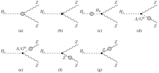
Figure 4: Generic diagrams contributing to the virtual corrections of the decay $H_{i}\to ZZ$: vertex corrections (a) and corrections to the external legs (c)-(g), where $k=1,2,3$. Diagram (b) displays the vertex counterterm.

The generic diagrams describing the virtual corrections contributing to the NLO decay width together with the counterterm diagram introduced to cancel the UV divergences are displayed in Fig. 4. With the decay width involving only neutral particles there are neither IR divergences nor real corrections. The corrections to the external legs in Fig. 4 (c), (f) and (g) vanish due to the OS renormalization of $H_{i}$ and $Z$, respectively, and the mixing contributions (d) and (e) are zero because of the Ward identity satisfied by the OS $Z$ boson. The one-particle irreducible (1PI) diagrams contributing to the vertex corrections originate from the triangle diagrams with scalars, fermions, massive gauge bosons and ghost particles in the loops, depicted in the first three rows of Fig. 5, and from the diagrams involving four-particle vertices, as given by the last four diagrams of Fig. 5.

Figure 5: Generic diagrams contributing to the vertex corrections in $H_{i}\to ZZ$ with fermions $F$, scalar bosons $S$, gauge bosons $V$ and ghost particles $U$ in the loops.

To work out the vertex counterterms, the relations

$$s_{\varphi}\to s_{\varphi}+c_{\varphi}\,\delta\varphi\qquad\mbox{and}\qquad c_{\varphi}\to c_{\varphi}-s_{\varphi}\,\delta\varphi$$ (6.168)

are helpful for the derivation of the entries in the rotation matrix counterterm $\delta R$ obtained from Eq. (2.29),

$$\delta R_{11} =-c_{\alpha_{1}}\,s_{\alpha_{2}}\delta_{\alpha_{2}}-s_{\alpha_{1}}c_{\alpha_{2}}\delta_{\alpha_{1}}$$

$$\delta R_{12} =-s_{\alpha_{1}}s_{\alpha_{2}}\delta_{\alpha_{2}}+c_{\alpha_{2}}c_{\alpha_{1}}\delta_{\alpha_{1}}$$

$$\delta R_{13} =c_{\alpha_{2}}\delta_{\alpha_{2}}$$

$$\delta R_{21} =-c_{\alpha_{1}}c_{\alpha_{3}}\delta_{\alpha_{1}}+s_{\alpha_{1}}s_{\alpha_{3}}\delta_{\alpha_{3}}-c_{\alpha_{1}}(s_{\alpha_{2}}c_{\alpha_{3}}\delta_{\alpha_{3}}+s_{\alpha_{3}}c_{\alpha_{2}}\delta_{\alpha_{2}})+s_{\alpha_{2}}s_{\alpha_{3}}s_{\alpha_{1}}\delta_{\alpha_{1}}$$

$$\delta R_{22} =-c_{\alpha_{1}}s_{\alpha_{3}}\delta_{\alpha_{3}}-s_{\alpha_{1}}c_{\alpha_{3}}\delta_{\alpha_{3}}-s_{\alpha_{1}}(s_{\alpha_{2}}c_{\alpha_{3}}\delta_{\alpha_{3}}+s_{\alpha_{3}}c_{\alpha_{2}}\delta_{\alpha_{2}})-c_{\alpha_{1}}s_{\alpha_{2}}s_{\alpha_{3}}\delta_{\alpha_{1}}$$

$$\delta R_{23} =-s_{\alpha_{2}}s_{\alpha_{3}}\delta_{\alpha_{2}}+c_{\alpha_{2}}c_{\alpha_{3}}\delta_{\alpha_{3}}$$

$$\delta R_{31} =s_{\alpha_{1}}c_{\alpha_{3}}\delta_{\alpha_{3}}+c_{\alpha_{1}}s_{\alpha_{3}}\delta_{\alpha_{1}}-c_{\alpha_{1}}(c_{\alpha_{2}}c_{\alpha_{3}}\delta_{\alpha_{2}}-s_{\alpha_{2}}s_{\alpha_{3}}\delta_{\alpha_{3}})+s_{\alpha_{1}}s_{\alpha_{2}}c_{\alpha_{3}}\delta_{\alpha_{1}}$$

$$\delta R_{32} =s_{\alpha_{1}}s_{\alpha_{3}}\delta_{\alpha_{1}}-c_{\alpha_{1}}s_{\alpha_{3}}\delta_{\alpha_{3}}+s_{\alpha_{1}}s_{\alpha_{2}}s_{\alpha_{3}}\delta_{\alpha_{3}}-c_{\alpha_{3}}(s_{\alpha_{1}}c_{\alpha_{2}}\delta_{\alpha_{2}}+c_{\alpha_{1}}s_{\alpha_{2}}\delta_{\alpha_{1}})$$

$$\delta R_{33} =-s_{\alpha_{2}}c_{\alpha_{3}}\delta_{\alpha_{2}}-c_{\alpha_{2}}s_{\alpha_{3}}\delta_{\alpha_{3}}\,.$$ (6.169)

The $H_{i}ZZ$ vertex counterterm in terms of the different parameter counterterms and wave function renormalization constants is obtained from the corresponding counterterm Lagrangian

$${\cal L}^{\text{ct}}_{H_{i}ZZ} =\left(\cfrac{gm_{Z}^{2}\,\kappa_{H_{i}ff}}{m_{W}}\,\left[\cfrac{\delta m_{Z}^{2}}{m_{Z}^{2}}\,-\left(\frac{\delta m_{W}^{2}}{2m_{W}^{2}}-\frac{\delta g}{g}\right)+\delta Z_{ZZ}+\cfrac{1}{2}\,\delta Z_{H_{i}H_{i}}+\cfrac{1}{2}\,\sum_{j\neq i}\cfrac{\kappa_{H_{j}VV}}{\kappa_{H_{i}VV}}\,\delta Z_{H_{j}H_{i}}\,\right]\right.$$

$$\left.\quad+\cfrac{gm_{Z}^{2}}{m_{W}}\,\left[\delta R_{i1}\,c_{\beta}+\delta R_{i2}\,s_{\beta}-(R_{i1}\,s_{\beta}-R_{i2}\,c_{\beta})\delta\beta\right]\right)g^{\mu\nu}H_{i}Z_{\mu}Z_{\nu}\,,$$ (6.170)

with the various counterterms given in Section 3 and the $\delta R_{ij}$ defined in Eq. (6.169). Since we apply the alternative tadpole scheme, tadpole contributions to the $H_{i}ZZ$ vertex have to be taken into account explicitly in the computation of the decay width. They are shown in Fig. 6. The formulae for the vertex corrections and counterterms in terms of the scalar one-, two- and three-point functions are quite lengthy so that we do not display them explicitly here.

Figure 6: Tadpole contributions to the vertex diagrams to be included in the decay $H_{i}\to ZZ$ in the alternative tadpole scheme.

6.2 The decay $H_{i}\to AA$ at NLO EW

The LO decay width of the CP-even $H_{i}$ decay into a pair of CP-odd scalars,

$$H_{i}\to AA\;,$$ (6.171)

reads

$$\Gamma^{\text{LO}}(H_{i}\to AA)=\frac{\alpha\,\left|\lambda_{H_{i}AA}\right|^{2}}{8s^{2}_{W}\,\,m_{H_{i}}}\sqrt{1-\frac{4m_{A}^{2}}{m_{H_{i}}^{2}}}\;.$$ (6.172)

It is governed by the trilinear coupling

$$g_{H_{i}AA}=-i\,\cdot\,\lambda_{H_{i}AA}\, =g\,\cfrac{1}{2m_{W}}\Bigg{\{}-M^{2}\left[\frac{R_{i1}}{c_{\beta}}+\frac{R_{i2}}{s_{\beta}}\right]+m_{H_{i}}^{2}\,\left[\frac{R_{i1}s_{\beta}^{2}}{c_{\beta}}+\frac{R_{i2}\,c_{\beta}^{2}}{s_{\beta}}\right]$$

$$\qquad+2\,m_{A}^{2}\,\left[R_{i1}c_{\beta}+R_{i2}s_{\beta}\right]\Bigg{\}}\;,$$ (6.173)

where $M^{2}\equiv m^{2}_{12}/(s_{\beta}c_{\beta})$.

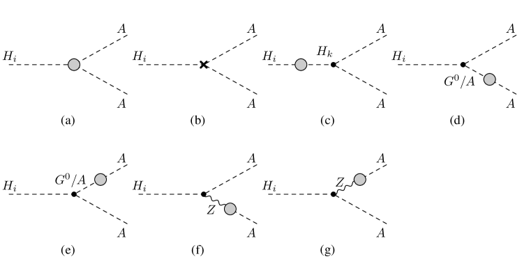
Figure 7: Generic diagrams contributing to the virtual corrections of the decay $H_{i}\to AA$: vertex corrections (a) and corrections to the external legs (c)-(g). Diagram (b) displays the corresponding vertex counterterm.

Figure 8: Generic diagrams contributing to the vertex corrections in $H_{i}\to AA$.

Figure 9: Tadpole contributions to the vertex diagrams to be included in the decay $H_{i}\to AA$ in the alternative tadpole scheme.

The EW one-loop corrections consist of the virtual corrections and the counterterm contributions ensuring the UV-finiteness of the decay amplitude. Again we do not have to deal with IR divergences nor real corrections. The virtual corrections, consisting of the corrections to the external legs and the pure vertex corrections, are shown in Fig. 7. The corrections to the external legs in Fig. 7 (c), (d) and (e) are zero because of the OS renormalization of the external fields, while diagrams (f) and (g) vanish due to a Slavnov-Taylor identity [64]. The 1PI diagrams of the vertex corrections are depicted in Fig. 8. They are given by the triangle diagrams with fermions, scalars and gauge bosons in the loops and by the diagrams containing four-particle vertices. The counterterm contributions consist of the genuine vertex counterterm $\delta g_{H_{i}AA}^{\text{vertex}}$ and the counterterm insertions on the external legs $\delta g_{H_{i}AA}^{\text{field}}$,

$$\delta g_{H_{i}AA} =\delta\,g^{\text{field}}_{H_{i}AA}+\delta\,g^{\text{vertex}}_{H_{i}AA}\,,$$ (6.174)

with

$$\delta\,g^{\text{field}}_{H_{i}AA} =g_{H_{i}AA}\,\left[\delta Z_{AA}+\frac{1}{2}\,\delta Z_{H_{i}H_{i}}+\frac{1}{2}\,\sum_{i\neq j}\,\cfrac{g_{H_{j}AA}}{g_{H_{i}AA}}\,\delta Z_{H_{j}H_{i}}+\cfrac{g_{H_{i}AG}}{g_{H_{i}AA}}\,\delta Z_{G^{0}A}\right]$$ (6.175)

and

$$\delta\,g^{\text{vertex}}_{H_{i}AA}= -g_{H_{i}AA}\,\left(\frac{\delta m_{W}^{2}}{2m_{W}^{2}}-\frac{\delta g}{g}\right)+\cfrac{g}{2m_{W}}\Bigg{\{}\left(R_{i1}\cfrac{s^{2}_{\beta}}{c_{\beta}}+R_{i2}\cfrac{c^{2}_{\beta}}{s_{\beta}}\right)\,\delta m^{2}_{H_{i}}-\left(\cfrac{R_{i1}}{c_{\beta}}+\cfrac{R_{i2}}{s_{\beta}}\right)\,\delta M^{2}$$

$$+2\,\left[R_{i1}c_{\beta}+R_{i2}s_{\beta}\right]\,\delta m_{A}^{2}-M^{2}\,\left(\cfrac{\delta R_{i1}}{c_{\beta}}+\cfrac{\delta R_{i2}}{s_{\beta}}\right)+m^{2}_{H_{i}}\,\left(\cfrac{s^{2}_{\beta}}{c_{\beta}}\,\delta R_{i1}+\cfrac{c^{2}_{\beta}}{s_{\beta}}\,\delta R_{i2}\right)\,$$

$$+2\,m_{A}^{2}\,\left[c_{\beta}\delta R_{i1}+s_{\beta}\delta R_{i2}\right]+M^{2}\,\left(R_{i1}\cfrac{\delta c_{\beta}}{c_{\beta}^{2}}+R_{i2}\cfrac{\delta s_{\beta}}{s_{\beta}^{2}}\right)+2\,m_{A}^{2}\,\left[R_{i1}\delta c_{\beta}+R_{i2}\,\delta s_{\beta}\right]$$

$$+m_{H_{i}}^{2}\,\left[R_{i1}\,\cfrac{s^{2}_{\beta}}{c_{\beta}}\left(2\cfrac{\delta s_{\beta}}{s_{\beta}}-\cfrac{\delta c_{\beta}}{c_{\beta}}\right)+R_{i2}\,\cfrac{c^{2}_{\beta}}{s_{\beta}}\left(2\cfrac{\delta c_{\beta}}{c_{\beta}}-\cfrac{\delta s_{\beta}}{s_{\beta}}\right)\right]\Bigg{\}}\,,$$ (6.176)

with the $\delta R_{ij}$ given in Eq. (6.169). Working in the alternative tadpole scheme, we additionally have to take into account the vertices dressed with the tadpoles, displayed in Fig. 9.

The one-loop correction to the decay is obtained from the interference of the loop-corrected decay amplitude ${\cal M}_{H_{i}AA}^{\text{1loop}}$ with the LO amplitude ${\cal M}_{H_{i}AA}^{\text{LO}}$. The one-loop amplitude combines the virtual corrections ${\cal M}_{H_{i}AA}^{\text{virt}}$, including external leg and pure vertex corrections, and the counterterm amplitude ${\cal M}_{H_{i}AA}^{\text{ct}}=\delta g_{H_{i}AA}+{\cal M}_{H_{i}AA}^{\text{tad}}$, with ${\cal M}_{H_{i}AA}^{\text{tad}}$ denoting the vertices with the tadpoles,

$${\cal M}_{H_{i}AA}^{\text{1loop}}={\cal M}_{H_{i}AA}^{\text{virt}}+{\cal M}^{\text{ct}}_{H_{i}AA}\;.$$ (6.177)

The NLO corrections factorise from the LO amplitude so that the loop-corrected partial width can be cast into the form

$$\Gamma^{\text{NLO}} =\Gamma^{\text{LO}}+\frac{m_{H_{i}}}{32\pi}\sqrt{1-\frac{4m_{A}^{2}}{m_{H_{i}}^{2}}}\,2\,\mbox{Re}\left[({\cal M}_{H_{i}AA}^{\text{LO}})^{*}{\cal M}_{H_{i}AA}^{\text{1loop}}\right]$$

$$=\Gamma^{\text{LO}}\,[1+\Delta^{\text{virt}}_{H_{i}AA}+\Delta^{\text{ct}}_{H_{i}AA}]\;,$$ (6.178)

with

$$\Delta^{\text{virt/ct}}_{H_{i}AA}\equiv\frac{2{\cal M}^{\text{virt/ct}}_{H_{i}AA}}{g_{H_{i}AA}}=\frac{2{\cal M}^{\text{virt/ct}}_{H_{i}AA}}{-i\cdot\lambda_{H_{i}AA}}\;.$$ (6.179)

Again we refrain from giving the explicit expressions for the various contributions to $\Gamma^{\text{NLO}}$ as they are quite lengthy.

6.3 Electroweak one-loop corrections to $H_{j}\to H_{i}H_{i}$

The LO decay width for the decay of a neutral CP-even Higgs boson into two identical CP-even scalars is given by ($i,j=1,2,3$ )

$$\Gamma^{\text{LO}}(H_{j}\to H_{i}H_{i})=\frac{\alpha\,\left|\lambda_{H_{i}H_{i}H_{j}}\right|^{2}}{8\,s^{2}_{W}\,m_{H_{j}}}\sqrt{1-\frac{4m_{H_{i}}^{2}}{m_{H_{j}}^{2}}}\;,$$ (6.180)

with the trilinear Higgs coupling

$$g_{H_{i}H_{i}H_{j}}\, =-i\cdot\lambda_{H_{i}H_{i}H_{j}}\,=\cfrac{g}{2m_{W}}\,\Bigg{\{}-\cfrac{1}{2}\,M^{2}\,\left[\left(\cfrac{R_{i2}}{s_{\beta}}-\cfrac{R_{i1}}{c_{\beta}}\right)\,\left(6R_{i2}R_{j2}\,c_{\beta}^{2}-6R_{i1}R_{j1}\,s_{\beta}^{2}\right.\right.$$

$$\left.\left.+\sum_{k}\,\epsilon_{ijk}\,R_{k3}\,s_{2\beta}\right)\right]+\cfrac{2m^{2}_{H_{i}}+m^{2}_{H_{j}}}{v_{S}}\,\left[R^{2}_{i3}\,R_{j3}\,v+R^{2}_{i2}\,R_{j2}\,\cfrac{v_{S}}{s_{\beta}}+R^{2}_{i1}\,R_{j1}\,\cfrac{v_{S}}{c_{\beta}}\right]\Bigg{\}}\;,$$ (6.181)

where $\epsilon_{ijk}$ denotes the totally antisymmetric tensor in three dimensions with $\epsilon_{123}=1$. At variance with the processes discussed so far, Higgs-to-Higgs decays in the CP-even sector are directly sensitive to the singlet VEV $v_{S}$ at tree level. As discussed in section 4.1, this explicit dependence must be handled with care when the NLO calculations are performed in the alternative tadpole scheme. Here, a non-vanishing UV-divergent singlet VEV shift $\Delta v_{S}$ cancels a subset of the UV poles in the NLO Higgs-to-Higgs decay amplitude which genuinely arise in this scheme. To fix $\Delta v_{S}$ we proceed along the same lines as for the doublet VEV. First, we identify the singlet VEV input value in this scheme with the (would-be) experimental input, to be extracted eventually through the measurement of an observable Higgs-to-Higgs decay width $\Gamma_{H_{i}\to H_{j}H_{j}}$. When promoted to higher orders, the tree-level relation $v^{\text{tree}}_{S}=f(\Gamma^{\text{tree}}_{H_{i}\to H_{j}H_{j}})$ becomes

$$\left.v^{\text{ren}}_{S}\right|_{\text{FJ}}=v_{S}^{\text{tree}}=f(\Gamma^{\text{tree}}_{H_{i}\to H_{j}H_{j}}) =f(\Gamma^{\text{ren}}_{H_{i}\to H_{j}H_{j}}+\Gamma^{\text{ct}}_{H_{i}\to H_{j}H_{j}})=\underbrace{\tilde{f}(\Gamma^{\text{ren}}_{H_{i}\to H_{j}H_{j}})}_{v_{S}^{\text{exp.}}}+\underbrace{\delta\tilde{f}(\Gamma^{\text{ct}}_{H_{i}\to H_{j}H_{j}})}_{\Delta v_{S}}\,,$$ (6.182)

in such a way that the (would-be) experimental value $v_{S}^{\text{exp}}$ is properly written in terms of the renormalized (physical) width from which it would be extracted. Notice that the quantity $\Delta v_{S}$ is simply a shorthand for the combination of counterterm contributions contained in $\Gamma^{\text{ct}}_{H_{i}\to H_{j}H_{j}}$ - the same role that $\Delta v$ plays in Eq. (4.48) for the doublet VEV case. For our sample processes $H_{3}\to H_{2}H_{2}$ and $H_{2}\to H_{1}H_{1}$ discussed in the numerical analysis we assume the $v_{S}$ input values to be extracted from the decay $H_{3}\to H_{1}H_{1}$. The choice of this process is of course not unique. Therefore, given that the finite parts included in $\Delta v_{S}$ are to some degree arbitrary, we could formally resort to $\overline{\text{MS}}$-like conditions to fix $\Delta v_{S}$ by retaining only the UV-divergent parts contained in $\Gamma^{\text{ct}}_{H_{i}\to H_{j}H_{j}}$. In this case the $v_{S}$ input values could not be extracted directly from the experimental data. The relation to the to be measured $v^{\text{exp}}_{S}$ would be given by a scheme-dependent finite shift. In the process-dependent framework $\Delta v_{S}$ can be fixed through the requirement

$$\Gamma^{\text{NLO}}_{H_{3}\to H_{1}H_{1}} \stackrel{{\scriptstyle!}}{{=}}\Gamma^{\text{LO}}_{H_{3}\to H_{1}H_{1}}\,.$$ (6.183)

Factorising the NLO decay width as

$$\Gamma^{\text{NLO}}_{H_{3}\to H_{1}H_{1}} =\Gamma^{\text{LO}}_{H_{3}\to H_{1}H_{1}}\Big{[}1+\Delta^{\text{virt}}+\Delta^{\text{ct}}(\Delta v_{S}=0)+\Delta^{\text{ct}}(\Delta v_{S})\Big{]}\stackrel{{\scriptstyle!}}{{=}}\Gamma^{\text{LO}}_{H_{3}\to H_{1}H_{1}}\,$$ (6.184)

and isolating the $v_{S}$-dependent part of the corresponding self-interaction Lagrangian,

$$\mathcal{L}_{H_{1}H_{1}H_{3}}\supset\cfrac{1}{v_{S}}\,(2m^{2}_{H_{1}}+m^{2}_{H_{3}})\,R^{2}_{13}\,R_{33}\;,\quad\text{whereby}$$

$$\delta\mathcal{L}_{H_{1}H_{1}H_{3}}\supset-\cfrac{1}{v_{S}}\,(2m^{2}_{H_{1}}+m^{2}_{H_{3}})\,R^{2}_{13}\,R_{33}\,\cfrac{\Delta\,v_{S}}{v_{S}}\,,$$ (6.185)

the condition Eq. (6.184) leads to

$$\cfrac{\Delta v_{S}}{v_{S}} =\cfrac{g_{H_{i}H_{i}H_{j}}\,v_{S}}{2}\Big{[}(2m_{H_{1}}^{2}+m_{H_{3}}^{2})R^{2}_{13}\,R_{33}\,\Big{]}^{-1}\,\left[\Delta^{\text{virt}}+\Delta^{\text{CT}}(\Delta v_{S}=0)\right]\,.$$ (6.186)

The diagrams contributing to the virtual corrections of our process $H_{j}\to H_{i}H_{i}$ are shown in Fig. 10. The 1PI diagrams contributing to the vertex corrections are depicted in Fig. 11 and the tadpole diagrams are shown in Fig. 12. They have to be included in the alternative tadpole scheme.

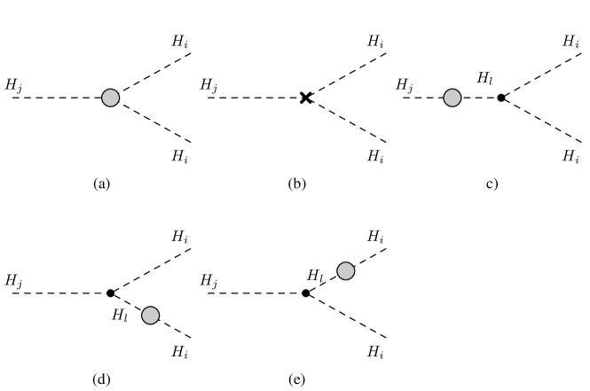
Figure 10: Generic diagrams contributing to the virtual corrections of the decay $H_{j}\to H_{i}H_{i}$: vertex corrections (a) and corrections to the external legs (c)-(e). Diagram (b) displays the corresponding vertex counterterm.

Figure 11: Generic diagrams contributing to the vertex corrections in $H_{j}\to H_{i}H_{i}$.

The counterterm is given by the genuine vertex counterterm and the counterterm insertions on the external legs,

$$\delta g_{H_{i}H_{j}H_{k}}=\delta\,g^{\text{field}}_{H_{i}H_{j}H_{k}}+\delta\,g^{\text{vertex}}_{H_{i}H_{j}H_{k}}\,,$$ (6.187)

with

$$\delta\,g^{\text{field}}_{H_{i}H_{j}H_{k}} = g_{H_{i}H_{j}H_{k}}\,\left[\frac{1}{2}\,\sum_{l=1}^{3}\,\cfrac{g_{H_{l}H_{j}H_{k}}}{g_{H_{i}H_{j}H_{k}}}\,\delta Z_{H_{l}H_{i}}+\frac{1}{2}\,\sum_{l=1}^{3}\,\cfrac{g_{H_{l}H_{i}H_{k}}}{g_{H_{i}H_{j}H_{k}}}\,\delta Z_{H_{l}H_{j}}\right.$$ (6.188)

$$\left.+\frac{1}{2}\,\sum_{l=1}^{3}\,\cfrac{g_{H_{l}H_{i}H_{j}}}{g_{H_{i}H_{j}H_{k}}}\,\delta Z_{H_{l}H_{k}}\right]\,,$$

and

$$\delta g_{H_{i}H_{j}H_{k}}^{\text{vertex}}= -g_{H_{i}H_{i}H_{j}}\,\left(\cfrac{\delta m_{W}^{2}}{2m_{W}^{2}}-\cfrac{\delta g}{g}\right)+\frac{1}{v}\,\Bigg{\{}-\cfrac{1}{2}\,\delta M^{2}\,\left[\left(\cfrac{R_{i2}}{s_{\beta}}-\cfrac{R_{i1}}{c_{\beta}}\right)\,\right.\times$$

$$\times\left.\left(6R_{i2}R_{j2}\,c_{\beta}^{2}-6R_{i1}R_{j1}\,s_{\beta}^{2}+\sum_{k}\,\epsilon_{ijk}\,R_{k3}\,s_{2\beta}\right)\right]$$

$$-\cfrac{1}{2}\,M^{2}\,\left[\left(\cfrac{\delta R_{i2}}{s_{\beta}}-\cfrac{\delta R_{i1}}{c_{\beta}}\right)\,\left(6R_{i2}R_{j2}\,c_{\beta}^{2}-6R_{i1}R_{j1}\,s_{\beta}^{2}+\sum_{k}\,\epsilon_{ijk}\,R_{k3}\,s_{2\beta}\right)\right]$$

$$-\cfrac{1}{2}\,M^{2}\,\left[\left(\cfrac{R_{i1}\,\delta c_{\beta}}{c^{2}_{\beta}}-\cfrac{R_{i2}\,\delta s_{\beta}}{s^{2}_{\beta}}\right)\,\left(6R_{i2}R_{j2}\,c_{\beta}^{2}-6R_{i1}R_{j1}\,s_{\beta}^{2}+\sum_{k}\,\epsilon_{ijk}\,R_{k3}\,s_{2\beta}\right)\right]$$

$$-\cfrac{1}{2}\,M^{2}\,\left(\cfrac{R_{i2}}{s_{\beta}}-\cfrac{R_{i1}}{c_{\beta}}\right)\,\Big{[}6R_{j2}c^{2}_{\beta}\delta R_{i2}+6R_{i2}c^{2}_{\beta}\delta R_{j2}+12R_{i2}R_{j2}c_{\beta}\delta c_{\beta}-6R_{i1}s^{2}_{\beta}\delta R_{j1}$$

$$-6R_{i1}s^{2}_{\beta}\delta R_{j1}-12R_{i1}R_{j1}s_{\beta}\delta s_{\beta}+\sum_{k}\,\epsilon_{ijk}\,(s_{\beta}\,\delta R_{k3}+2R_{k3}\,(c_{\beta}\delta s_{\beta}+s_{\beta}\delta c_{\beta})\Big{]}$$

$$+\cfrac{2\delta m^{2}_{H_{i}}+\delta m^{2}_{H_{j}}}{v_{S}}\,\left[R^{2}_{i3}\,R_{j3}\,v+R^{2}_{i2}\,R_{j2}\,\cfrac{v_{S}}{s_{\beta}}+R^{2}_{i1}\,R_{j1}\,\cfrac{v_{S}}{c_{\beta}}\right]$$

$$-\cfrac{v}{v_{S}}\,(2m^{2}_{H_{i}}+m^{2}_{H_{j}})\,R^{2}_{i3}\,R_{j3}\,\cfrac{\Delta\,v_{S}}{v_{S}}+\cfrac{2m^{2}_{H_{i}}+m^{2}_{H_{j}}}{v_{S}}\,\Big{[}2R_{i3}\,R_{j3}\,v\,\delta R_{i3}+R^{2}_{i3}\,v\,\delta R_{j3}$$

$$+R^{2}_{i3}\,R_{j3}\,\delta v+2R_{i2}\,R_{j2}\,\cfrac{v_{S}}{s_{\beta}}\delta R_{i2}+R^{2}_{i2}\,\cfrac{v_{S}}{s_{\beta}}\delta R_{j2}-R^{2}_{i2}\,R_{j2}\,\cfrac{v_{S}}{s^{2}_{\beta}}\delta s_{\beta}+2R_{i1}\,R_{j1}\,\cfrac{v_{S}}{c_{\beta}}\delta R_{i1}$$

$$+R^{2}_{i1}\,\cfrac{v_{S}}{c_{\beta}}\delta R_{j1}-R^{2}_{i1}\,R_{j1}\,\cfrac{v_{S}}{c^{2}_{\beta}}\,\delta c_{\beta}\Big{]}\Bigg{\}}\,.$$ (6.189)

The NLO corrections factorise so that the loop-corrected decay width can be cast into the form

$$\Gamma^{\text{NLO}} =\Gamma^{\text{LO}}\,[1+\Delta^{\text{virt}}_{H_{i}H_{j}H_{k}}+\Delta^{\text{ct}}_{H_{i}H_{j}H_{k}}]\;,$$ (6.190)

with

$$\Delta^{\text{virt/ct}}_{H_{i}H_{j}H_{k}}\equiv\frac{2{\cal M}^{\text{virt/ct}}_{H_{i}H_{j}H_{k}}}{g_{H_{i}H_{j}H_{k}}}=\frac{2{\cal M}^{\text{virt/ct}}_{H_{i}H_{j}H_{k}}}{-i\cdot\lambda_{H_{i}H_{j}H_{k}}}$$ (6.191)

in terms of the virtual corrections and counterterm amplitude ${\cal M}^{\text{virt}}_{H_{i}H_{j}H_{k}}$ and ${\cal M}^{\text{ct}}_{H_{i}H_{j}H_{k}}$, respectively, where we have included the vertices with the tadpoles in ${\cal M}^{\text{ct}}_{H_{i}H_{j}H_{k}}$. Due to rather lengthy expressions we refrain from giving the explicit expressions of the various contributions to $\Gamma^{\text{NLO}}$.

Figure 12: Tadpole contributions to the vertex diagrams to be included in the decay $H_{j}\to H_{i}H_{i}$ in the alternative tadpole scheme.

7 Numerical Analysis

For the computation of the NLO EW corrections to the Higgs decays presented in the following the tree-level and one-loop decay amplitudes have been generated with FeynArts [66, 67]. The necessary N2HDM Feynman rules have been obtained as UFO [68] and FeynArts [67] model files using FeynRules[69], while all renormalization counterterms have been derived analytically and implemented by hand. The amplitudes have been analytically processed via FormCalc [70]. The dimensionally regularised loop form factors have been evaluated in the ’t Hooft-Veltman scheme [71, 72] and written in terms of standard loop integrals. These have been further reduced through Passarino-Veltman decomposition and evaluated with the help of LoopTools [70].

In the following we give the input parameters for the numerical evaluation. As explained in section 5 we use the fine structure constant $\alpha$ at the $Z$ boson mass scale, given by [73]

$$\alpha(m_{Z}^{2})=\frac{1}{128.962}\;.$$ (7.192)

The massive gauge bosons are renormalized OS, and their input masses are chosen as [73, 74]

$$m_{W}=80.385\mbox{ GeV}\qquad\mbox{and}\qquad m_{Z}=91.1876\mbox{ GeV}\;.$$ (7.193)

For the lepton masses we take [73, 74]

$$m_{e}=0.510998928\mbox{ MeV}\;,\quad m_{\mu}=105.6583715\mbox{ MeV}\;,\quad m_{\tau}=1.77682\mbox{ GeV}\;.$$ (7.194)

These and the light quark masses, which we set [75]

$$m_{u}=100\mbox{ MeV}\;,\quad m_{d}=100\mbox{ MeV}\;,\quad m_{s}=100\mbox{ MeV}\;,$$ (7.195)

have only a small impact on our results. Following the recommendation of the LHC Higgs Cross Section Working Group (HXSWG) [74, 76], we use the following OS value for the top quark mass

$$m_{t}=172.5\mbox{ GeV}\;,$$ (7.196)

which is consistent with the ATLAS and CMS analyses. The charm and bottom quark OS masses are set to

$$m_{c}=1.51\mbox{ GeV}\qquad\mbox{and}\qquad m_{b}=4.92\mbox{ GeV}\;,$$ (7.197)

as recommended by [74]. We consider the CKM matrix to be unity. This approximation has negligible impact on our results. The SM-like Higgs mass value, denoted by $m_{h}$, has been set to [26]

$$m_{h}=125.09\mbox{ GeV}\;.$$ (7.198)

Note that, depending on the parameter set, in the N2HDM any of the three neutral CP-even Higgs bosons can be the SM-like Higgs boson.

In the subsequently presented analysis we only used N2HDM parameter sets compatible experimental and theoretical constraints. These data sets have been generated with the tool ScannerS [30, 31]. The applied theoretical constraints require that the vacuum state found by ScannerS is the global minimum, that the N2HDM potential is bounded from below and that tree-level unitarity holds. On the experimental side, compatibility with the EW precision constraints is guaranteed by requiring the oblique parameters $S$, $T$ and $U$ to be compatible with the SM fit [77] at $2\sigma$, including the full correlations. The constraints from $B$ physics observables [78, 79, 80, 81, 82] and the measurement of $R_{b}$ [79, 83] have been taken into account, as well as the most recent bound of $m_{H^{\pm}}\raisebox{-3.69899pt}{~{}\shortstack{$>$ \\ [-0.07cm] $\sim$}}~{}580$ GeV for the type II and flipped (N)2HDM [82]. For the compatibility with the LHC Higgs data we require one of the scalar states, denoted by $h_{125}$, to have a mass of 125.09 GeV and to match the observed LHC signal rates. Furthermore, the remaining Higgs bosons have to be consistent with the exclusion bounds from the collider searches at Tevatron, LEP and LHC. For further details on these checks and the scan, we refer to [21, 22].

Note that in all scenarios presented in the following we stick to the N2HDM type I, with the type II scenarios leading to the same overall results. The only difference between the models comes from the fermion loops. The Yukawa couplings are, in all Yukawa types, well-behaved functions of the $\alpha_{i}$ and $\beta$ because extreme values of $\beta$ are already disallowed by all the constraints imposed on the model. Therefore, this is sufficient for our analysis to illustrate the effects of the EW corrections, without aiming at a full phenomenological analysis of N2HDM Higgs decays.

7.1 Results for $H_{2/3}\to ZZ$

In this section we investigate the relative size of the NLO EW corrections as well as the impact of the different renormalization schemes for the mixing angles on the decay $H_{i}\to ZZ$. We base our numerical analysis upon a set of representative N2HDM scenarios of phenomenological interest. To this aim we select among the generated parameter points compatible with the theoretical and experimental constraints scenarios that either have a large or a small LO branching fraction (BR) into $ZZ$. Discarding the SM-like decay of the $H_{1}$ fixed to be the 125 GeV Higgs boson, we select hence four scenarios, two for $H_{2}$ and $H_{3}$, respectively, which we denote by ’BRH2/3high’ and ’BRH2/3low’ for high and low branching ratio scenarios. The corresponding input parameters are listed in Table 6. Note that, if not stated otherwise, the mixing angles are understood to be the angles defined in the OS tadpole pinched scheme (pOS) with $\delta\beta$ defined via the charged sector, denoted by the superscript ’$c$’. The suppressed branching fractions in the BRlow scenarios are due to a small tree-level coupling to $ZZ$ of the decaying Higgs boson. The branching fractions given in this table have been obtained with the Fortran code N2HDECAY. We insured to consider purely OS decays into massive gauge bosons in N2HDECAY, as we do not include any gauge boson off-shell effects in the NLO computation.

	BRH2ZZhigh	BRH3ZZhigh	BRH2ZZlow	BRH3ZZlow
$m_{H_{1}}$	125.09	125.09	125.09	125.09
$m_{H_{2}}$	673.70	600.76	657.07	283.53
$m_{H_{3}}$	692.22	713.74	658.28	751.72
$m_{A}$	669.07	743.00	543.62	763.09
$m_{H^{\pm}}$	679.76	695.73	528.76	733.05
$t_{\beta}$ (pOSc)	6.12	8.39	4.79	3.53
$\alpha_{1}$ (pOS)	-1.513	-1.526	-1.489	1.318
$\alpha_{2}$ (pOS)	0.098	-0.308	0.225	0.0362
$\alpha_{3}$ (pOS)	-0.495	-1.421	-1.001	1.504
$m^{2}_{12}$	74518.4	60125.0	87240.8	143579.0
$v_{s}$	305.48	854.50	834.33	219.29
$\Gamma_{H}$	2.946	2.241	2.990	2.746
BR	0.327	0.329	0.010	0.010

Table 6: Input parameters for the N2HDM benchmark scenarios used in the numerical analysis of the decay processes $H_{2/3}\to ZZ$. In round brackets we specify the scheme in which $\alpha$ and $\beta$ are defined. All masses and $v_{S}$ are given in GeV. The LO total width (also given in GeV) and individual branching fractions in the last two rows correspond to the Higgs state and decay each benchmark is named after, and have been generated with N2HDECAY.

		pOSc	pOSo	p${}_{\star}^{c}$	p${}_{\star}^{o}$
BRH2ZZhigh	$\Gamma^{\text{LO}}(H_{2}\to ZZ)$	0.989	0.989	1.008	1.008
	$\Gamma^{\text{NLO}}(H_{2}\to ZZ)$	1.120	1.122	1.142	1.148
	$\Delta\Gamma^{H_{2}ZZ}$ [%]	13.2	13.4	13.3	14.0
BRH3ZZhigh	$\Gamma^{\text{LO}}(H_{3}\to ZZ)$	0.755	0.755	0.782	0.782
	$\Gamma^{\text{NLO}}(H_{3}\to ZZ)$	0.872	0.867	0.890	0.889
	$\Delta\Gamma^{H_{3}ZZ}$ [%]	15.6	14.9	13.9	13.7
BRH2ZZlow	$\Gamma^{\text{LO}}(H_{2}\to ZZ)$	3.130$\times 10^{-2}$	3.130$\times 10^{-2}$	2.529$\times 10^{-2}$	2.533$\times 10^{-2}$
	$\Gamma^{\text{NLO}}(H_{2}\to ZZ)$	3.042$\times 10^{-2}$	3.040$\times 10^{-2}$	2.840$\times 10^{-2}$	2.745$\times 10^{-2}$
	$\Delta\Gamma^{H_{2}ZZ}$ [%]	-2.8	-2.9	12.3	8.4
BRH3ZZlow	$\Gamma^{\text{LO}}(H_{3}\to ZZ)$	2.870$\times 10^{-2}$	2.869$\times 10^{-2}$	3.430$\times 10^{-2}$	3.418$\times 10^{-2}$
	$\Gamma^{\text{NLO}}(H_{3}\to ZZ)$	2.990$\times 10^{-2}$	3.011$\times 10^{-2}$	3.593$\times 10^{-2}$	3.738$\times 10^{-2}$
	$\Delta\Gamma^{H_{3}ZZ}$ [%]	4.2	5.0	4.8	9.3

Table 7: Higgs decay widths (in GeV) at LO and NLO EW accuracy as well as the relative corrections for the N2HDM benchmarks presented in Table 6 and four different renormalization schemes.

In Table 7 we present for all four benchmark scenarios the results for the LO and the NLO width as well as the relative corrections $\Delta\Gamma$. They are given for four different renormalization schemes. These consist of the p_⋆ and the pOS tadpole pinched schemes, which employ two different renormalization scales, and for these additionally the two possibilities to renormalize $\beta$, either via the charged sector (denoted by ’$c$’) or the CP-odd sector (denoted by ’$o$’). The relative corrections are defined as

$$\Delta\Gamma\equiv\frac{\Delta\Gamma^{\text{NLO}}}{\Gamma^{\text{LO}}}=\frac{\Gamma^{\text{NLO}}-\Gamma^{\text{LO}}}{\Gamma^{\text{LO}}}\;.$$ (7.199)

When computing the NLO EW corrected decay width $\Gamma^{\text{NLO}}$ in a different renormalization scheme $b$ than the one of the input parameters $p$, scheme $a$, these parameters first have to be converted to the scheme that is applied. We perform this conversion for the mixing angles $\alpha$ and $\beta$ through ($p=\alpha,\beta$)

$$p^{b}=p^{a}+\delta p^{a}-\delta p^{b}\;,$$ (7.200)

where $\delta p$ denotes the counterterm in either scheme $a$ or scheme $b$. With the thus obtained input parameters in scheme $b$ we compute the quantity $\Delta\Gamma^{\text{NLO}}$ and the LO width $\Gamma^{\text{LO}}$, to which we normalize the relative correction.

The relative corrections for the scenarios with relatively large branching ratios turn out to be of moderate size with values between 13.2 and 15.6%. The variation due to different renormalization schemes is at most 1.9%, indicating a relatively small theoretical error due to missing higher order corrections. For the low branching ratio scenarios on the other hand, the differences between the results for the various renormalization schemes are substantial. This points towards a large theoretical error due to missing higher order corrections. A reliable prediction in these cases would require the inclusion of corrections beyond one-loop order. This is to be expected as the tree-level widths are very small in these scenarios so that the one-loop correction effectively becomes the leading contribution to the width. When changing from the charged to the CP-odd based renormalization of $\beta$, the change in the relative corrections is rather mild for most of the scenarios. This is because the two different scales, $m_{H^{\pm}}$ or $m_{A}$, involved in these two renormalization schemes of $\beta$ are close in our scenarios.

7.2 Results for $H_{2/3}\to AA$

	BRH2AAhigh	BRH3AAhigh	BRH2AAlow	BRH3AAlow
$m_{H_{1}}$	125.09	125.09	125.09	125.09
$m_{H_{2}}$	130.48	137.15	294.92	243.70
$m_{H_{3}}$	347.65	146.22	503.44	903.07
$m_{A}$	58.14	70.27	74.28	429.82
$m_{H^{\pm}}$	146.93	166.83	278.19	426.18
$t_{\beta}$ (pOSc)	5.89	5.55	6.12	4.01
$\alpha_{1}$ (pOS)	-1.535	1.338	-1.457	1.409
$\alpha_{2}$ (pOS)	0.369	0.095	-0.117	-0.195
$\alpha_{3}$ (pOS)	0.029	-1.28	-0.118	-0.078
$m^{2}_{12}$ ($\mu_{R}=2m_{A}$)	864.2	982.9	13036.9	8300.6
$v_{s}$	538.37	638.95	1352.51	991.00
$\Gamma_{H}$	2.694	2.005	4.986 $\cdot 10^{-2}$	26.140 $\cdot 10^{-2}$
BR	0.999	0.999	0.997	0.992

Table 8: Input parameters for the N2HDM benchmarks used in the numerical analysis of the decay process $H_{2/3}\to AA$. All masses and $v_{S}$ are given in GeV. The LO total width (also given in GeV) and individual branching fractions in the last two rows correspond to the Higgs state and decay each benchmark is named after, and have been generated with N2HDECAY.

Here we study the decay into a pair of pseudoscalars and again concentrate on the decays of the heavier Higgs bosons $H_{2}$ and $H_{3}$ and choose scenarios where $H_{1}$ is the 125 GeV Higgs boson and with low and high branching ratios for $H_{2/3}\to AA$, respectively. The corresponding benchmark scenarios are called ’BRH2/3AAhigh’ and ’BRH2/3AAlow’, with the input values summarised in Tab. 8 together with the LO total widths and branching ratios computed with N2HDECAY. The input mixing angles are given in the pOS scheme and the $\beta$ renormalization is based on the charged sector. The parameter $m_{12}^{2}$ is assumed to be given at the scale $\mu_{R}=2m_{A}$. The suppressed decay widths in the BRlow scenarios are due to a small trilinear coupling $\lambda_{H_{2/3}AA}$. In the BRhigh scenarios, the $H_{2/3}\to AA$ decays are maximised because $(i)$ the $H_{2/3}AA$ trilinear couplings are enhanced, $(ii)$ the couplings to fermions are suppressed and $(iii)$ the decays into massive weak bosons are kinematically closed.

		pOSc	pOSo	p${}_{\star}^{c}$	p${}_{\star}^{o}$
BRH2AAhigh	$\Gamma^{\text{Born}}(H_{2}\to AA)$	2.761	2.759	2.761	2.760
	$\Gamma^{\text{NLO}}(H_{2}\to AA)$	2.454	2.500	2.459	2.500
	$\Delta\Gamma^{H_{2}AA}$ [%]	-11.1	-9.4	-10.9	-9.4
BRH3AAhigh	$\Gamma^{\text{Born}}(H_{3}\to AA)$	2.054	2.053	2.042	2.041
	$\Gamma^{\text{NLO}}(H_{3}\to AA)$	1.840	1.885	1.848	1.886
	$\Delta\Gamma^{H_{3}AA}$ [%]	-10.4	-8.1	-9.5	-7.6
BRH2AAlow	$\Gamma^{\text{Born}}(H_{2}\to AA)$	5.097$\times 10^{-2}$	5.266$\times 10^{-2}$	5.075$\times 10^{-2}$	5.208$\times 10^{-2}$
	$\Gamma^{\text{NLO}}(H_{2}\to AA)$	5.408$\times 10^{-2}$	-1.013$\times 10^{-2}$	4.071$\times 10^{-2}$	-9.986$\times 10^{-3}$
	$\Delta\Gamma^{H_{2}AA}$ [%]	6.1	-119.2	-19.8	-119.2
BRH3AAlow	$\Gamma^{\text{Born}}(H_{3}\to AA)$	0.266	0.266	0.286	0.286
	$\Gamma^{\text{NLO}}(H_{3}\to AA)$	0.277	0.272	0.270	0.277
	$\Delta\Gamma^{H_{3}AA}$ [%]	4.4	2.1	-5.5	-3.0

Table 9: Higgs decay widths (in GeV) at LO and NLO EW accuracy as well as the relative corrections for the N2HDM benchmarks presented in Table 8 and four different renormalization schemes. The renormalization scale of $m_{12}^{2}$ is set to $\mu_{R}=2m_{A}$.

In Table 9 we display for all four benchmark scenarios the LO and NLO widths as well as the relative corrections $\Delta\Gamma$. They are given for the four different renormalization schemes, p${}_{\star}^{c/o}$, pOS^c/o. As can be inferred from the table, for the BRhigh scenarios we obtain moderate corrections of $\mathcal{O}(10)\%$, i.e. of the same order as for $H_{2/3}\to ZZ$. The associated theoretical uncertainties are very mild, as indicated by the the rather small influence of the renormalization schemes of the mixing angles, which lead to a change of at most 2.8%, when considering all four schemes. The $H_{2/3}\to AA$ decays in the BRlow scenarios, on the contrary, are dominated by the loop effects. Here, the small trilinear Higgs coupling suppresses the tree-level width. At one loop, however, the Higgs decay is also sensitive to the additional trilinear Higgs couplings, some of which being very large as a result of the heavy Higgs masses and the large $m^{2}_{12}$ scale - yet in agreement with the unitarity constraints. This results in very large NLO effects, and also induces the strong dependence on the renormalization scheme and the renormalization scale. This reflects the fact that the $H_{2/3}\to AA$ decays in these benchmarks are effectively loop-induced and higher order corrections beyond the one-loop level need to be considered to make reliable predictions. These sizable higher-order effects are particularly apparent in the BRH2AAlow scenario, where some of the renormalization schemes even lead to negative and hence unphysical NLO widths. Note, furthermore, that the change when switching from the charged to the CP-odd based renormalization schemes for $\beta$ is now larger when compared to the results in Table 7, due to the now wider separation between the scales given by the charged and the CP-odd Higgs mass as compared to the scenarios studied for the decays into a $Z$ boson pair.

7.3 Results for $H_{3}\to H_{2}\,H_{2}$ and $H_{2}\to H_{1}H_{1}$

	HHHI	HHHII	HHHIII	HHHIV
$m_{H_{1}}$	125.09	125.09	125.09	125.09
$m_{H_{2}}$	304.18	425.61	351.65	298.42
$m_{H_{3}}$	630.94	857.27	717.32	743.18
$m_{A}$	325.07	547.48	487.07	362.40
$m_{H^{\pm}}$	265.81	383.85	386.42	306.19
$t_{\beta}$ (pOSc)	6.30	5.17	4.08	6.26
$\alpha_{1}$ (pOS)	-1.559	1.495	1.453	1.315
$\alpha_{2}$ (pOS)	-0.330	0.082	0.353	-0.148
$\alpha_{3}$ (pOS)	-0.077	-0.101	0.340	-0.098
$m^{2}_{12}$ ($\mu_{R}=2m_{H_{\text{final}}}$)	14312.1	32824.5	35765.3	12707.3
$v_{s}$	1327.57	1098.81	630.19	1425.0
$\Gamma_{H_{3}}$	24.160	25.190	43.590	18.750
BR($H_{3}\to H_{1}H_{1}$)	0.13	0.03	0.08	0.08
BR($H_{3}\to H_{2}H_{2}$)	0.05	0.10	0.15	0.15
$\Gamma_{H_{2}}$	0.393	0.723	1.558	0.234
BR($H_{2}\to H_{1}H_{1}$)	0.17	0.47	0.43	0.76

Table 10: Input parameters for the N2HDM benchmarks used in the numerical analysis of the decay processes $H_{j}\to H_{i}H_{i}$. All masses and $v_{S}$ are given in GeV. In the last five rows the total $H_{2}$ and $H_{3}$ widths are given in GeV as well as the branching fractions (generated with N2HDECAY) of the Higgs-to-Higgs decays $H_{3}\to H_{1}H_{1},H_{2}H_{2}$ and $H_{2}\to H_{1}H_{1}$.

		pOSc	pOSo	p${}_{\star}^{c}$	p${}_{\star}^{o}$
HHHI	$\Gamma(H_{3}\to H_{1}H_{1})$	3.206	3.206	3.197	3.197
	$\Gamma^{\text{LO}}(H_{3}\to H_{2}H_{2})$	1.229	1.229	1.242	1.242
	$\Gamma^{\text{NLO}}(H_{3}\to H_{2}H_{2})$	1.344	1.343	1.344	1.341
	$\Delta\Gamma^{H_{3}\to H_{2}H_{2}}$ [%]	9.4	9.3	8.2	8.0
	$\Gamma^{\text{LO}}(H_{2}\to H_{1}H_{1})$	$6.699\times 10^{-2}$	$6.699\times 10^{-2}$	$6.667\times 10^{-2}$	$6.667\times 10^{-2}$
	$\Gamma^{\text{NLO}}(H_{2}\to H_{1}H_{1})$	$7.433\times 10^{-2}$	$7.429\times 10^{-2}$	$7.429\times 10^{-2}$	$7.409\times 10^{-2}$
	$\Delta\Gamma^{H_{2}\to H_{1}H_{1}}$ [%]	11.0	10.9	11.4	11.1
HHHII	$\Gamma(H_{3}\to H_{1}H_{1})$	0.719	0.719	0.753	0.753
	$\Gamma^{\text{LO}}(H_{3}\to H_{2}H_{2})$	2.580	2.580	2.730	2.730
	$\Gamma^{\text{NLO}}(H_{3}\to H_{2}H_{2})$	2.453	2.454	2.493	2.492
	$\Delta\Gamma^{H_{3}\to H_{2}H_{2}}$ [%]	-4.9	-4.9	-8.7	-8.7
	$\Gamma^{\text{LO}}(H_{2}\to H_{1}H_{1})$	0.345	0.345	0.343	0.343
	$\Gamma^{\text{NLO}}(H_{2}\to H_{1}H_{1})$	0.398	0.398	0.397	0.397
	$\Delta\Gamma^{H_{2}\to H_{1}H_{1}}$ [%]	15.2	15.2	15.9	15.9
HHHIII	$\Gamma(H_{3}\to H_{1}H_{1})$	3.561	3.561	3.565	3.564
	$\Gamma^{\text{LO}}(H_{3}\to H_{2}H_{2})$	6.662	6.661	6.469	6.466
	$\Gamma^{\text{NLO}}(H_{3}\to H_{2}H_{2})$	6.071	6.094	6.208	6.264
	$\Delta\Gamma^{H_{3}\to H_{2}H_{2}}$ [%]	-8.883	-8.515	-4.027	-3.118
	$\Gamma^{\text{LO}}(H_{2}\to H_{1}H_{1})$	0.687	0.687	0.684	0.683
	$\Gamma^{\text{NLO}}(H_{2}\to H_{1}H_{1})$	0.678	0.679	0.675	0.676
	$\Delta\Gamma^{H_{2}\to H_{1}H_{1}}$ [%]	-1.3	-1.2	-1.3	-1.1
HHHIV	$\Gamma(H_{3}\to H_{1}H_{1})$	1.446	1.446	1.422	1.422
	$\Gamma^{\text{LO}}(H_{3}\to H_{2}H_{2})$	2.873	2.874	2.860	2.859
	$\Gamma^{\text{NLO}}(H_{3}\to H_{2}H_{2})$	2.793	2.780	2.799	2.820
	$\Delta\Gamma^{H_{3}\to H_{2}H_{2}}$ [%]	-2.8	-3.3	-2.1	-1.4
	$\Gamma^{\text{LO}}(H_{2}\to H_{1}H_{1})$	0.183	0.183	0.185	0.185
	$\Gamma^{\text{NLO}}(H_{2}\to H_{1}H_{1})$	0.151	0.144	0.147	0.158
	$\Delta\Gamma^{H_{2}\to H_{1}H_{1}}$ [%]	-17.4	-21.3	-20.6	-14.3

Table 11: Higgs decay width predictions (in GeV) at LO and NLO EW accuracy as well as the relative corrections for the N2HDM benchmarks presented in Table 10 and four different renormalization schemes.

Finally, we consider the decay of a heavy neutral CP-even Higgs boson into a pair of lighter CP-even Higgs bosons. We evaluate the NLO EW corrections for a number of illustrative scenarios, given in Table 10. The scenarios have been chosen such that their Higgs mass spectra allow simultaneously for the OS $H_{3}\to H_{2}H_{2}$ and $H_{2}\to H_{1}H_{1}$ decays. Furthermore, the chosen large $m^{2}_{12}$ parameter insures these heavy Higgs mass scenarios to be in agreement with the unitarity and vacuum stability constraints. All scenarios feature Higgs-to-Higgs decay branching ratios that are of moderate size. Only HHHIV features a $H_{2}$ branching ratio into $H_{1}H_{1}$ that is dominating. All input mixing angles are assumed to be given in the pOS scheme, with charged sector-based renormalization for the angle $\beta$, and $m_{12}^{2}$ is assumed to be defined at the renormalization scale given by the total final state mass, $\mu_{R}=2m_{H_{i}}$. The LO total widths and branching ratios in this table have been obtained from N2HDECAY.

In Table 11 we summarise the relative NLO corrections for the various decays. Note, that the decay process $H_{3}\to H_{1}H_{1}$ appears only at LO because we use it for the renormalization of $v_{S}$, as explained in detail in Section 6. The sizeable $m^{2}_{12}$ and heavy Higgs mass values imply large Higgs self-couplings and thereby enhanced contributions from the virtual Higgs exchanges. On the other hand, these enhancements are partly damped by the inverse Higgs mass powers in the Higgs-mediated loops. The balance between these dynamical features governing the Higgs-mediated loops, and how they interplay with the remaining gauge boson and fermion-mediated one-loop contributions, determines the overall size of the NLO EW effects. For most of the decays, the relative NLO corrections are moderate and reach at most 21%. Accordingly, they show a mild renormalization scheme and scale dependence with changes in the predicted NLO widths typically at the percent level or below. Some decays, however, exhibit a stronger renormalization scheme and scale dependence. This implies a larger theoretical uncertainty and can be explained by the mass hierarchies and couplings governing these cases, which lead to loop-dominated decays.

8 Conclusions

In this paper we worked out the renormalization of the N2HDM, which is an interesting benchmark model for studying extended Higgs sectors involving Higgs-to-Higgs decays. For the mixing angles, we provided a renormalization scheme that is manifestly gauge independent by applying the alternative tadpole scheme combined with the pinch technique. We explained in great detail the notion of the alternative tadpole scheme in our renormalization framework, and for the first time provided the formulae for the pinched self-energies in the N2HDM. Apart from the additional mixing angles as compared to the 2HDM, in the N2HDM we encounter a singlet VEV that needs to be renormalized as well. We elaborated in detail the implications of the alternative tadpole scheme for the renormalization of the singlet VEV that we renormalize through a physical quantity, given by a Higgs-to-Higgs decay width. The soft $\mathbb{Z}_{2}$ breaking parameter $m_{12}^{2}$, which, like $v_{S}$, enters the Higgs self-couplings and hence features in Higgs-to-Higgs decays, is renormalized in the $\overline{\mbox{MS}}$ scheme. We studied the impact of our renormalization scheme by computing the EW one-loop corrections to various Higgs decay widths, including the Higgs decays into a massive $Z$-boson pair and into lighter Higgs pairs.

The computation of the EW corrections to our different sample decay widths has shown that the corrections can be sizeable and have to be taken into account in order to make reliable predictions for the Higgs observables. For a broad range of phenomenologically representative scenarios we find a rather weak renormalization scale and renormalization scheme dependence, indicative of a rather small theoretical error due to missing higher order corrections. In some cases the EW corrections can be sizeable, in particular if the corresponding LO decay widths are suppressed, so that the NLO-corrected width effectively becomes the leading order decay width. Higher order corrections beyond NLO would then be necessary in order to reduce the theoretical error.

With this paper, we have provided an important contribution to the renormalization of extended Higgs sectors involving singlet fields. This is crucial input for the computation of the EW corrections to the Higgs bosons of such models and therefore indispensable for the correct prediction and interpretation of Higgs observables at the LHC.

Acknowledgments

The authors acknowledge financial support from the DFG project “Precision Calculations in the Higgs Sector - Paving the Way to the New Physics Landscape” (ID: MU 3138/1-1). We would like to thank Marco Sampaio, Michael Spira and Jonas Wittbrodt for useful discussions.

Appendix

Appendix A The Pinch Technique in the N2HDM

In this section, we present the explicit gauge dependences appearing in the scalar-scalar and scalar-vector self-energies in the N2HDM. Additionally, we present the application of the pinch technique in the N2HDM for the first time, as well as the cancellation of all gauge dependences by the generation of pinched self-energies.

A.1 Gauge dependence of the self-energies

We begin by setting the notation used in the explicit expressions of the gauge dependences. Following the notation of Ref. [59], we define the functions

$$f_{\Phi_{i}\Phi_{j}}(p^{2}) =p^{2}-\frac{m_{\Phi_{i}}^{2}+m_{\Phi_{j}}^{2}}{2}$$ (A.1)

$$g_{\Phi_{i}\Phi_{j}}(p^{2},m^{2}) =2\left(p^{2}-m^{2}\right)\left(p^{2}-\frac{m_{\Phi_{i}}^{2}+m_{\Phi_{j}}^{2}}{2}\right)-\left(p^{2}-m_{\Phi_{i}}^{2}\right)\left(p^{2}-m_{\Phi_{j}}^{2}\right)~{},$$ (A.2)

where $\Phi$ stands for an arbitrary neutral or charged scalar particle and $m_{\Phi_{i,j}}=0$ in case $\Phi_{i,j}$ is a Goldstone boson. We introduce the one-loop integrals

$$\alpha_{V} =\frac{1}{\left(1-\xi_{V}\right)m_{V}^{2}}\left[A_{0}\left(m_{V}^{2}\right)-A_{0}\left(\xi_{V}m_{V}^{2}\right)\right]=B_{0}\left(0;m_{V}^{2},\xi_{V}m_{V}^{2}\right)$$ (A.3)

$$\beta_{V\Phi_{i}}(p^{2}) =\frac{1}{\left(1-\xi_{V}\right)m_{V}^{2}}\left[B_{0}\left(p^{2};m_{V}^{2},m_{\Phi_{i}}^{2}\right)-B_{0}\left(p^{2};\xi_{V}m_{V}^{2},m_{\Phi_{i}}^{2}\right)\right]$$ (A.4)

$$=C_{0}\left(0,p^{2},p^{2};m_{V}^{2},\xi_{V}m_{V}^{2},m_{\Phi_{i}}^{2}\right)$$

$$\beta_{V\xi V}(p^{2}) =\frac{1}{\left(1-\xi_{V}\right)m_{V}^{2}}\left[B_{0}\left(p^{2};m_{V}^{2},\xi_{V}m_{V}^{2}\right)-B_{0}\left(p^{2};\xi_{V}m_{V}^{2},\xi_{V}m_{V}^{2}\right)\right]$$ (A.5)

$$=C_{0}\left(0,p^{2},p^{2};\xi_{V}m_{V}^{2},\xi_{V}m_{V}^{2},m_{\Phi_{i}}^{2}\right)$$

$$C_{2}^{V\Phi_{i}}(p^{2}) =C_{2}\left(0,p^{2},p^{2};m_{V}^{2},\xi_{V}m_{V}^{2},m_{\Phi_{i}}^{2}\right)~{},$$ (A.6)

where $A_{0}$, $B_{0}$ and $C_{0}$ denote the usual scalar one-, two- and three-point integrals and $C_{2}$ denotes the coefficient integral of the tensor integral $C_{\mu}$, which can be expressed solely through $A_{0}$ and $B_{0}$ integrals, cf. Refs. [61, 49]. The index $V$ denotes a vector boson $V\in\left\{W^{\pm},Z,\gamma\right\}$.

In what follows, we extract the gauge dependences of all self-energies via the definition

$$i\Sigma^{\text{tad}}(p^{2})=\left.i\Sigma^{\text{tad}}(p^{2})\right|_{\xi_{V}=1}+\left.i\Sigma(p^{2})\right|_{\text{g.d.}}\;,$$ (A.7)

where $i\Sigma^{\text{tad}}(p^{2})$ is the fully gauge-dependent modified self-energy with tadpole contributions included, cf. Fig. 3, $\left.i\Sigma(p^{2})\right|_{\text{g.d.}}$ represents the truly gauge-dependent part of the self-energy and $\left.i\Sigma(p^{2})\right|_{\xi_{V}=1}$ denotes the evaluation of the self-energy in the ’t-Hooft Feynman gauge. The inclusion of tadpole contributions for the analysis of the self-energies with respect to gauge dependence is necessary for a consistent application of the pinch technique [52]. While the extraction of the gauge dependence via Eq. (A.7) is not unique, we show in the following by applying the pinch technique that $\left.i\Sigma(p^{2})\right|_{\text{g.d.}}$ is considered to be the truly gauge-dependent part of the self-energies, since it is precisely these terms which are cancelled by the pinch contributions.

A.1.1 Gauge dependence of the CP-even scalar self-energies

Figure 13: All Feynman diagrams contributing to the gauge dependence of the CP-even self-energies $\Sigma^{\text{tad}}_{H_{i}H_{j}}(p^{2})$. For the tadpole diagram, a sum over intermediate Higgs states $H_{k}$ $(k=1,2,3$) is assumed. Note that the ghost and vector boson contributions in the tadpole diagrams precisely cancel against each other, so that these are not shown.

First, we consider the gauge dependence of the CP-even scalar self-energies, i.e. the self-energies of all possible combinations of $H_{i}$ and $H_{j}$ ($i,j=1,2,3$). All Feynman diagrams contributing gauge-dependent terms are shown in Fig. 13. The evaluation of Eq. (A.7) for the CP-even scalars of the N2HDM sector yields

$$\begin{split}i\Sigma^{\text{tad}}_{H_{i}H_{j}}(p^{2})&=\left.i\Sigma^{\text{tad}}_{H_{i}H_{j}}(p^{2})\right|_{\xi_{V}=1}\\ &+\frac{ig^{2}\left(1-\xi_{Z}\right)}{64\pi^{2}\cos\Theta_{W}}\bigg{[}g_{H_{i}H_{j}}(p^{2},m_{A}^{2})\mathcal{O}^{(1)}_{H_{i}H_{j}}\beta_{ZA}(p^{2})-f_{H_{i}H_{j}}(p^{2})\mathcal{O}^{(4)}_{H_{i}H_{j}}\alpha_{Z}\\ &\hskip 76.82234pt+\frac{1}{2}g_{H_{i}H_{j}}(p^{2},0)\mathcal{O}^{(2)}_{H_{i}H_{j}}\left(\beta_{ZZ}(p^{2})+\beta_{Z\xi Z}(p^{2})\right)\bigg{]}\\ &+\frac{ig^{2}\left(1-\xi_{W}\right)}{32\pi^{2}}\bigg{[}g_{H_{i}H_{j}}(p^{2},m_{H^{\pm}}^{2})\mathcal{O}^{(1)}_{H_{i}H_{j}}\beta_{WH^{\pm}}(p^{2})-f_{H_{i}H_{j}}(p^{2})\mathcal{O}^{(4)}_{H_{i}H_{j}}\alpha_{W}\\ &\hskip 76.82234pt+\frac{1}{2}g_{H_{i}H_{j}}(p^{2},0)\mathcal{O}^{(2)}_{H_{i}H_{j}}\left(\beta_{WW}(p^{2})+\beta_{W\xi W}(p^{2})\right)\bigg{]}~{},\end{split}$$ (A.8)

where the combinations $\mathcal{O}^{(1)}_{H_{i}H_{j}}$, $\mathcal{O}^{(2)}_{H_{i}H_{j}}$ and $\mathcal{O}^{(4)}_{H_{i}H_{j}}$ have been defined in Eq. (5.151). We note that when evaluating these combinations in the 2HDM limit, i.e. by applying Eq. (2.55), where $\mathcal{O}^{(4)}_{H_{i}H_{j}}$ reduces to the Kronecker delta $\delta_{H_{i}H_{j}}$, the result in Eq. (A.8) coincides with the results presented in Refs. [60, 40] for the 2HDM as well as with the result presented in Ref. [59] for the MSSM, since the structure of the gauge-dependence of the CP-even scalar self-energies does not differ between the MSSM and the 2HDM.

A.1.2 Gauge dependence of the charged scalar and vector self-energies

Figure 14: All Feynman diagrams contributing to the gauge-dependence of the charged self-energies $\Sigma^{\text{tad}}_{\phi^{\pm}_{i}\phi^{\pm}_{j}}(p^{2})$ where $\phi^{\pm}_{i,j}\in\{W,G^{\pm},H^{\pm}\}$. A sum over intermediate Higgs states $H_{k}$ is assumed wherever they appear. Overlapping dashed and twiggled lines denote a scalar or a gauge boson, respectively, depending on the chosen particles. Note that we only consider contributions to the extended scalar sector of the N2HDM. Depending on the particles $\phi^{\pm}_{i,j}$ chosen, some of the diagrams shown may not exist in the N2HDM.

Next, we consider the charged sector. Due to the mixing of the charged particles of the N2HDM, we have to consider not only all possible self-energy combinations of the scalar particles $H^{\pm}$ and $G^{\pm}$, but additionally their mixing with the charged vector bosons $W^{\pm}$. In the SM, where only one Higgs boson exists, it was shown that the Higgs contributions to the gauge dependence of the charged sector form a gauge-dependent subset which is cancelled by a corresponding subset of pinch contributions [56]. In the N2HDM we follow the same approach, i.e. we focus only on gauge-dependent contributions stemming from the enriched scalar sector of the N2HDM, which form a subset with respect to gauge dependence as well.

We first consider the gauge dependence of the self-energies of all combinations of $W^{\pm}$ and $G^{\pm}$. The relevant contributions from the Higgs sector are given by the Feynman diagrams in Fig. 14 for all possible self-energies. Note that since we consider only the subset where the scalars of the N2HDM appear in the loops, only terms containing the gauge-fixing parameter $\xi_{W}$ contribute to these self-energies. They explicitly read

$$i\Sigma^{\text{tad}}_{WW,\mu\nu}(p^{2}) =\left.i\Sigma^{\text{tad}}_{WW,\mu\nu}(p^{2})\right|_{\xi_{V}=1}$$ (A.9)

$$-(1-\xi_{W})\frac{ig^{2}m_{W}^{2}}{64\pi^{2}}p_{\mu}p_{\nu}\sum_{H_{i}}\mathcal{O}^{(2)}_{H_{i}H_{i}}\left\{\beta_{WH_{i}}(p^{2})+4C_{2}^{WH_{i}}(p^{2})\right\}$$

$$i\Sigma^{\text{tad}}_{WG^{\pm},\mu}(p^{2}) =\left.i\Sigma^{\text{tad}}_{WG^{\pm},\mu}(p^{2})\right|_{\xi_{V}=1}$$ (A.10)

$$+(1-\xi_{W})\frac{ig^{2}m_{W}}{64\pi^{2}}p_{\mu}\left\{\alpha_{W}+\sum_{H_{i}}\mathcal{O}^{(2)}_{H_{i}H_{i}}\left[m_{H_{i}}^{2}\beta_{WH_{i}}(p^{2})+2p^{2}C_{2}^{WH_{i}}(p^{2})\right]\right\}$$

$$i\Sigma^{\text{tad}}_{G^{\pm}G^{\pm}}(p^{2}) =\left.i\Sigma^{\text{tad}}_{G^{\pm}G^{\pm}}(p^{2})\right|_{\xi_{V}=1}$$ (A.11)

$$+(1-\xi_{W})\frac{ig^{2}}{64\pi^{2}}\left\{-2f_{G^{\pm}G^{\pm}}(p^{2})\alpha_{W}+\sum_{H_{i}}\mathcal{O}^{(2)}_{H_{i}H_{i}}g_{G^{\pm}G^{\pm}}(p^{2},m_{H_{i}}^{2})\beta_{WH_{i}}(p^{2})\right\}\;.$$

Next, the gauge dependence of the self-energies of all combinations of $H^{\pm}$ and $G^{\pm}$ or $W^{\pm}$ is given by the relevant contributions from the Higgs sector as given by the Feynman diagrams in Fig. 14 as well. In the case of the self-energy for two $H^{\pm}$ particles, additional dependences on $\xi_{Z}$ and $\xi_{\gamma}$ appear even when focusing on the extended scalar sector of the N2HDM only, while for the other self-energies only the dependence on $\xi_{W}$ is relevant. The self-energies explicitly read

$$i\Sigma^{\text{tad}}_{H^{\pm}H^{\pm}}(p^{2}) =\left.i\Sigma^{\text{tad}}_{H^{\pm}H^{\pm}}(p^{2})\right|_{\xi_{V}=1}$$ (A.12)

$$+(1-\xi_{W})\frac{ig^{2}}{64\pi^{2}}\left\{-2f_{H^{\pm}H^{\pm}}(p^{2})\alpha_{W}+g_{H^{\pm}H^{\pm}}(p^{2},m_{A}^{2})\beta_{WA}\right.$$

$$+\sum_{H_{i}}\mathcal{O}^{(2)}_{H_{i}H_{i}}g_{H^{\pm}H^{\pm}}(p^{2},m_{H_{i}}^{2})\beta_{WH_{i}}\big{\}}$$

$$+(1-\xi_{Z})\frac{ig^{2}(\cos^{2}\Theta_{W}-\sin^{2}\Theta_{W})^{2}}{64\pi^{2}\cos^{2}\Theta_{W}}\left\{g_{H^{\pm}H^{\pm}}(p^{2},m_{H^{+}}^{2})\beta_{ZH^{\pm}}(p^{2})-f_{H^{\pm}H^{\pm}}(p^{2})\alpha_{Z}\right\}$$

$$+(1-\xi_{\gamma})\frac{ie^{2}}{16\pi^{2}}\left\{-f_{H^{\pm}H^{\pm}}(p^{2})\alpha_{\gamma}+g_{H^{\pm}H^{\pm}}(p^{2},m_{H^{+}}^{2})\beta_{\gamma H^{\pm}}(p^{2})\right\}$$

$$i\Sigma^{\text{tad}}_{H^{\pm}G^{\pm}}(p^{2}) =\left.i\Sigma^{\text{tad}}_{H^{\pm}G^{\pm}}(p^{2})\right|_{\xi_{V}=1}$$ (A.13)

$$+(1-\xi_{W})\frac{ig^{2}}{64\pi^{2}}\sum_{H_{i}}\mathcal{O}^{(3)}_{H_{i}H_{i}}g_{H^{\pm}G^{\pm}}(p^{2},m_{H_{i}}^{2})\beta_{WH_{i}}(p^{2})$$

$$i\Sigma^{\text{tad}}_{WH^{\pm},\mu}(p^{2}) =\left.i\Sigma^{\text{tad}}_{WH^{\pm},\mu}(p^{2})\right|_{\xi_{V}=1}$$ (A.14)

$$-(1-\xi_{W})\frac{ig^{2}m_{W}}{64\pi^{2}}p_{\mu}\sum_{H_{i}}\mathcal{O}^{(3)}_{H_{i}H_{i}}\left\{f_{H^{\pm}H^{\pm}}(m_{H_{i}}^{2})\beta_{WH_{i}}(p^{2})+2f_{H^{\pm}H^{\pm}}(p^{2})C_{2}^{WH_{i}}(p^{2})\right\}$$

Note that when the former two equations are evaluated in the 2HDM-limit, cf. Eq. (2.55), these reproduce the formulae given in Ref. [40] for the 2HDM.

A.1.3 Gauge dependence of the CP-odd scalar and vector self-energies

Figure 15: All Feynman diagrams contributing to the gauge-dependence of the CP-odd self-energies $\Sigma^{\text{tad}}_{\phi^{0}_{i}\phi^{0}_{j}}(p^{2})$ where $\phi^{0}_{i,j}\in\{A,G^{0}\}$. A sum over intermediate Higgs states $H_{k}$ is assumed wherever they appear. Note that we only consider contributions to the extended scalar sector of the N2HDM. Depending on the particles $\phi^{0}_{i,j}$ chosen, some of the diagrams shown may not exist in the N2HDM.

In the neutral CP-odd sector the calculation of the gauge dependences and of the pinch contributions is even more involved than in the charged sector, since one has to take into account not only the mixing of the $Z$ boson with $G^{0}$ and $A$, but additionally the mixing of the photon $\gamma$ with all other possible contributions. It is only the coherent sum of all these mixing contributions which gives the correct gauge dependences and pinch results. Due to these additional complications, we restrict the presentation to the self-energies of two $A$ and the mixing between $A$ and $G^{0}$. As in the charged sector, we focus on the N2HDM Higgs contributions to the self-energies and pinch terms only, since they form a gauge-independent subset on their own. The relevant contributions are given by the Feynman diagrams in Fig. 15. In total, the self-energies of this subset read

$$i\Sigma^{\text{tad}}_{AA}(p^{2}) =\left.i\Sigma^{\text{tad}}_{AA}(p^{2})\right|_{\xi_{V}=1}$$ (A.15)

$$+(1-\xi_{Z})\frac{ig^{2}}{64\pi^{2}\cos^{2}\Theta_{W}}\left\{-f_{AA}(p^{2})\alpha_{Z}+\sum_{H_{i}}\mathcal{O}^{(1)}_{H_{i}H_{i}}g_{AA}(p^{2},m_{H_{i}}^{2})\beta_{ZH_{i}}(p^{2})\right\}$$

$$+(1-\xi_{W})\frac{ig^{2}}{32\pi^{2}}\left\{-f_{H^{\pm}H^{\pm}}(p^{2})\alpha_{W}+g_{AA}(p^{2},m_{H^{\pm}}^{2})\beta_{WH^{\pm}}(p^{2})\right\}$$

$$i\Sigma^{\text{tad}}_{AG^{0}}(p^{2}) =\left.i\Sigma^{\text{tad}}_{AG^{0}}(p^{2})\right|_{\xi_{V}=1}$$ (A.16)

$$+(1-\xi_{Z})\frac{ig^{2}}{64\pi^{2}\cos^{2}\Theta_{W}}\sum_{H_{i}}\mathcal{O}^{(3)}_{H_{i}H_{i}}g_{AG^{0}}(p^{2},m_{H_{i}}^{2})\beta_{ZH_{i}}(p^{2})~{}.$$

As in the charged sector, these results, evaluated in the 2HDM limit, reproduce the ones presented in Ref. [40] for the 2HDM.

A.2 Pinch contributions for the N2HDM

The intricate gauge dependence of the scalar self-energies of the N2HDM makes a gauge-independent definition of the counterterms of the scalar mixing angles complicated. If one considers instead an $S$-matrix element, e.g. a scattering process of a pair of fermions, where these self-energies may appear as intermediate states, the whole $S$-matrix element is gauge independent by construction. Consequently, the gauge dependences cancel in an intricate way between the self-energies and other contributions from vertex and box corrections within the $S$-matrix element.

The main idea of the pinch technique (cf. Refs. [51, 52, 53, 54, 55, 56, 57, 58] for a detailed exposition) is to isolate the gauge dependences of an arbitrary toy scattering process, which features the to-be pinched self-energies in a unique way. This is achieved by applying the elementary Ward identities

$$\not{k}\,P_{L/R} =S^{-1}_{1}(p+k)P_{L/R}-P_{R/L}S^{-1}_{2}(p)+m_{1}P_{L/R}-m_{2}P_{R/L}$$

$$P_{L/R}\,\not{k} =P_{L/R}S^{-1}_{1}(p+k)-S^{-1}_{2}(p)P_{R/L}+m_{1}P_{L/R}-m_{2}P_{R/L}~{},$$ (A.17)

where $k$ denotes the loop momentum, $m_{1}$ and $m_{2}$ the masses of the external fermions of the considered toy process and $S(p)$ the fermion propagator

$$iS_{k}(p)=\frac{i(\not{p}+m_{k})}{p^{2}-m_{k}^{2}}=\frac{i}{\not{p}-m_{k}}~{}.$$ (A.18)

It turns out that the gauge dependences are all similar in structure, i.e. they are always self-energy-like, independently of their origin within the scattering process. The isolation of all pinch contributions from the toy scattering process then allows for a manifestly gauge-independent definition of pinched self-energies. Since these self-energies are considered to be independent from the toy process chosen, cf. [52], the pinched self-energies are unique.

A.2.1 Pinch contributions for the CP-even sector

Figure 16: All generic Feynman diagrams contributing to the CP-even pinched self-energies.

The full derivation of all pinch contributions for the N2HDM is beyond the scope of this paper. We nevertheless present the derivation of the pinch contributions for a few selected diagrams since we hope it is instructive to the reader and since it demonstrates how the pinch technique is applied. As the toy process for extracting the gauge dependences for the CP-even sector we choose the process $\mu^{+}\mu^{-}\rightarrow\bar{b}b$. All Feynman diagrams yielding contributions for the CP-even pinched self-energies are depicted in Fig. 16. It can be shown that all pinch contributions stemming from these diagrams can be brought into the form

$$\Gamma^{H_{i}bb}\frac{i}{p^{2}-m_{H_{i}}^{2}}i\Sigma^{\text{PT}}_{H_{i}H_{j}}(p^{2})\frac{i}{p^{2}-m_{H_{j}}^{2}}\Gamma^{H_{j}\mu\mu}\;,$$ (A.19)

where $i\Sigma^{\text{PT}}_{H_{i}H_{j}}(p^{2})$ is a relevant self-energy-like pinch contribution for the CP-even Higgs bosons $H_{i}$ and $H_{j}$. Additionally, we define the contracted vertices of a CP-even Higgs boson with a pair of external bottom quarks or a pair of external muons as

$$\Gamma^{H_{i}bb}=\bar{u}(r_{1})\frac{-igm_{b}\kappa_{H_{i}bb}}{2m_{W}}v(r_{2})\qquad\mbox{and}\qquad\Gamma^{H_{i}\mu\mu}=\bar{v}(p_{2})\frac{-igm_{\mu}\kappa_{H_{i}\mu\mu}}{2m_{W}}u(p_{1})\;,$$ (A.20)

where $u(p_{1})$ and $v(r_{2})$ and $\bar{u}(r_{1})$ and $\bar{v}(p_{2})$ are the (adjoint) spinors of the external on-shell fermions with their respective momenta.

In order to derive the pinch contributions, we apply the elementary Ward identities, cf. Eq. (A.17), and insert additional CP-even Higgs boson propagators into the amplitude via

$$1=-\frac{i}{p^{2}-m_{H_{i}}^{2}}i(p^{2}-m_{H_{i}}^{2})~{}.$$ (A.21)

Additionally, we make use of the sum rules of the N2HDM as given in Eq. (5.152) as well as of the coupling relation

$$\kappa_{H_{i}ff}=\kappa_{H_{i}VV}-\tilde{\kappa}_{H_{i}VH}\kappa_{Aff}\;.$$ (A.22)

The application of these formulae to fermion-fermion-Higgs couplings enables the projection of the pinch contributions onto the desired CP-even Higgs couplings to the fermions,

$$\tilde{\kappa}\kappa_{All}=\sum_{H_{j}}\tilde{\kappa}\kappa_{H_{j}VV}\kappa_{All}\kappa_{H_{j}ll}=-\sum_{H_{j}}\mathcal{O}^{(1)}_{H_{i}H_{j}}\kappa_{H_{j}ll}\hskip 11.38092pt+\hskip 11.38092pt\text{...}$$ (A.23)

where “…” contains pinch contributions for other than the CP-even Higgs self-energies. Consequently, we can neglect them for the CP-even self-energies.

Figure 17: Two Feynman diagrams for the toy process $\mu^{+}\mu^{-}\rightarrow\bar{b}b$ involving scalar-scalar-vector vertices which give rise to gauge-dependent as well as additional gauge-independent pinch contributions for the CP-even self-energies. The momenta $p_{1}$ and $p_{2}$ are taken as incoming and the momenta $r_{1}$ and $r_{2}$ as outgoing, and $p=p_{1}+p_{2}$.

We consider the two contributions depicted in the Feynman diagrams in Fig. 17. The momenta are as defined in the diagrams. With the definitions given above, the sum of both diagrams reads

$$\begin{split}&\sum_{H_{i}}\Gamma^{H_{i}bb}\frac{i}{p^{2}-m_{H_{i}}^{2}}\frac{g^{2}}{32\pi^{2}}\int\frac{\text{d}^{4}k}{i\pi^{2}}\frac{1}{\left[k^{2}-m_{W}^{2}\right]\left[(k+p)^{2}-m_{H^{\pm}}^{2}\right]}\\ &\hskip 28.45274pt\cdot\bigg{\{}\bar{v}(p_{2})\left[P_{L}S_{\mu_{\nu}}(k+p_{1})(\not{k}+2\not{p})P_{L}+P_{R}(-\not{k}-2\not{p})S_{\mu_{\nu}}(-k-p_{2})P_{R}\right]\frac{igm_{\mu}}{2m_{W}}\kappa_{All}\tilde{\kappa}_{H_{i}VH}u(p_{1})\\ &\hskip 28.45274pt-(1-\xi_{W})\bar{v}(p_{2})\left[P_{L}S_{\mu_{\nu}}(k+p_{2})\not{k}P_{L}+P_{R}(-\not{k})S_{\mu_{\nu}}(-k-p_{2})P_{R}\right]\frac{igm_{\mu}}{2m_{W}}\kappa_{All}\tilde{\kappa}_{H_{i}VH}u(p_{1})\bigg{\}}\\ &\stackrel{{\scriptstyle(\ref{eq:pinchWardIdent})}}{{=}}\sum_{H_{i}}\Gamma^{H_{i}bb}\frac{i}{p^{2}-m_{H_{i}}^{2}}\frac{g^{2}}{32\pi^{2}}\bar{v}(p_{2})\frac{igm_{\mu}}{2m_{W}}\kappa_{All}\tilde{\kappa}_{H_{i}VH}u(p_{1})\Big{\{}B_{0}(p^{2};m_{W}^{2},m_{H^{\pm}}^{2})\\ &\hskip 28.45274pt-(1-\xi_{W})\left[\alpha_{W}-f_{H^{\pm}H^{\pm}}(p^{2})\beta_{WH^{\pm}}\right]\Big{\}}\hskip 11.38092pt+\hskip 11.38092pt\text{...}\\ &\stackrel{{\scriptstyle(\ref{eq:pinchSumRules})}}{{=}}\sum_{H_{i},H_{j}}\Gamma^{H_{i}bb}\frac{i}{p^{2}-m_{H_{i}}^{2}}\frac{-g^{2}}{32\pi^{2}}\mathcal{O}^{(1)}_{H_{i}H_{j}}\Big{\{}B_{0}(p^{2};m_{W}^{2},m_{H^{\pm}}^{2})\\ &\hskip 28.45274pt-(1-\xi_{W})\left[\alpha_{W}-f_{H^{\pm}H^{\pm}}(p^{2})\beta_{WH^{\pm}}\right]\Big{\}}\Gamma^{H_{j}\mu\mu}\hskip 11.38092pt+\hskip 11.38092pt\text{...}\\ &\stackrel{{\scriptstyle(\ref{eq:CPevenPropagators})}}{{=}}\sum_{H_{i},H_{j}}\Gamma^{H_{i}bb}\frac{i}{p^{2}-m_{H_{i}}^{2}}\frac{-ig^{2}}{16\pi^{2}}\left(\frac{p^{2}}{2}-\frac{m_{H_{j}}^{2}}{2}\right)\mathcal{O}^{(1)}_{H_{i}H_{j}}\Big{\{}B_{0}(p^{2};m_{W}^{2},m_{H^{\pm}}^{2})\\ &\hskip 28.45274pt-(1-\xi_{W})\left[\alpha_{W}-f_{H^{\pm}H^{\pm}}(p^{2})\beta_{WH^{\pm}}\right]\Big{\}}\frac{i}{p^{2}-m_{H_{j}}^{2}}\Gamma^{H_{j}\mu\mu}\hskip 11.38092pt+\hskip 11.38092pt\text{...}\\ &=\sum_{H_{i},H_{j}}\Gamma^{H_{i}bb}\frac{i}{p^{2}-m_{H_{i}}^{2}}i\Sigma^{\text{PT}}_{H_{i}H_{j}}(p^{2})\frac{i}{p^{2}-m_{H_{j}}^{2}}\Gamma^{H_{j}\mu\mu}\hskip 11.38092pt+\hskip 11.38092pt\text{...}\end{split}$$ (A.24)

The first term of the right-hand side of the Ward identities in Eq. (A.17) removes the internal fermion propagators from the loops, i.e. the fermions are pinched out, while the second term of the Ward identities vanishes due to the Dirac equation. The third and fourth terms produce pinch contributions to pinched vertices, but not to pinched self-energies. Consequently, these terms are collected in “…”, since they are of no interest for the generation of a pinched self-energy. The application of the sum rule in Eq. (A.23) produces additional pinch contributions to other self-energies than the CP-even ones due to different fermion-Higgs couplings. Consequently, these other terms are collected in “…” as well.

As mentioned before, the pinch contributions take the form of a self-energy and here they explicitly read

$$\begin{split}i\Sigma^{\text{PT}}_{H_{i}H_{j}}(p^{2})=\frac{-ig^{2}}{16\pi^{2}}\left(\frac{p^{2}}{2}-\frac{m_{H_{j}}^{2}}{2}\right)\mathcal{O}^{(1)}_{H_{i}H_{j}}\Big{\{}&B_{0}(p^{2};m_{W}^{2},m_{H^{\pm}}^{2})\\ &-(1-\xi_{W})\left[\alpha_{W}+(m_{H^{\pm}}^{2}-p^{2})\beta_{WH^{\pm}}\right]\Big{\}}\;.\end{split}$$ (A.25)

The terms proportional to $(1-\xi_{W})$ are gauge-dependent pinch contributions which cancel against parts of the gauge dependence of the CP-even self-energies. The other term which remains for $\xi_{W}=1$ is an additional gauge-independent pinch contribution which is specific to scalar-scalar-vector vertices in the vertex corrections [52, 59]. Repeating the calculation for the vertex corrections of the bottom quarks containing $H^{\pm}$ and $W^{\pm}$ bosons in the loop yields the same result as in Eq. (A.25), but with $m_{H_{j}}^{2}$ replaced by $m_{H_{i}}^{2}$. The combination of these results yields the first term in the second line of Eq. (5.148).

All Feynman diagrams contributing to the pinch terms for the CP-even sector are depicted in Fig. 16. Repeating the calculation as demonstrated above and combining all results leads to the pinch contributions to the CP-even sector,

$$\begin{split}i\Sigma^{\text{PT}}_{H_{i}H_{j}}(p^{2})&=i\Sigma^{\text{add}}_{H_{i}H_{j}}(p^{2})\\ &-\frac{ig^{2}\left(1-\xi_{Z}\right)}{64\pi^{2}\cos\Theta_{W}}\bigg{[}g_{H_{i}H_{j}}(p^{2},m_{A}^{2})\mathcal{O}^{(1)}_{H_{i}H_{j}}\beta_{ZA}(p^{2})-f_{H_{i}H_{j}}(p^{2})\mathcal{O}^{(4)}_{H_{i}H_{j}}\alpha_{Z}\\ &\hskip 76.82234pt+\frac{1}{2}g_{H_{i}H_{j}}(p^{2},0)\mathcal{O}^{(2)}_{H_{i}H_{j}}\left(\beta_{ZZ}(p^{2})+\beta_{Z\xi Z}(p^{2})\right)\bigg{]}\\ &-\frac{ig^{2}\left(1-\xi_{W}\right)}{32\pi^{2}}\bigg{[}g_{H_{i}H_{j}}(p^{2},m_{H^{\pm}}^{2})\mathcal{O}^{(1)}_{H_{i}H_{j}}\beta_{ZH^{\pm}}(p^{2})-f_{H_{i}H_{j}}(p^{2})\mathcal{O}^{(4)}_{H_{i}H_{j}}\alpha_{W}\\ &\hskip 76.82234pt+\frac{1}{2}g_{H_{i}H_{j}}(p^{2},0)\mathcal{O}^{(2)}_{H_{i}H_{j}}\left(\beta_{WW}(p^{2})+\beta_{W\xi W}(p^{2})\right)\bigg{]}~{}.\end{split}$$ (A.26)

By comparing this result with Eq. (A.8), we realize that in the sum of the pinch contributions with the CP-even self-energies all gauge-dependent terms proportional to $(1-\xi_{W})$ and $(1-\xi_{Z})$ precisely cancel, leading to

$$\overline{\Sigma}_{H_{i}H_{j}}(p^{2})=\Sigma^{\text{tad}}_{H_{i}H_{j}}(p^{2})+\Sigma^{\text{PT}}_{H_{i}H_{j}}(p^{2})=\left.\Sigma^{\text{tad}}_{H_{i}H_{j}}(p^{2})\right|_{\xi_{V}=1}+\Sigma^{\text{add}}_{H_{i}H_{j}}(p^{2})~{}.$$ (A.27)

Due to the cancellation of all gauge-dependent terms, the pinched self-energy $\overline{\Sigma}_{H_{i}H_{j}}(p^{2})$ is gauge independent by construction and equivalent to the self-energy evaluated in the Feynman gauge, together with the sum of all additional terms stemming from diagrams with internal scalar-scalar-vector vertices, as given in Eq. (5.148).

A.2.2 Pinch contributions for the charged sector

For the derivation of the pinch contributions of the charged sector we use the toy process $\nu_{e}e^{+}\rightarrow\nu_{e}e^{+}$. The calculation is analogous to the CP-even sector, i.e. we apply the elementary Ward identities from Eq. (A.17) and use the N2HDM sum rules to identify the correct couplings between the external fermions and the scalar or vector particles of interest. In the case of the self-energies involving the $H^{\pm}$ particles, we again insert the corresponding propagator by

$$1=-\frac{i}{p^{2}-m_{H^{\pm}}^{2}}i(p^{2}-m_{H^{\pm}}^{2})~{}.$$ (A.28)

For the self-energies involving $G^{\pm}$ or $W^{\pm}$, the corresponding propagators

$$\Delta_{\mu\nu}(p)\equiv\frac{-i}{p^{2}-m_{W}^{2}}\left[g_{\mu\nu}-(1-\xi_{W})\frac{p_{\mu}p_{\nu}}{p^{2}-\xi_{W}m_{W}^{2}}\right]\qquad\mbox{and}\qquad D(p)\equiv\frac{i}{p^{2}-\xi_{W}m_{W}^{2}}\,$$ (A.29)

are included into the pinch contributions by applying the identities [56]

$$g_{\nu\alpha} =i\left\{\Delta_{\nu\mu}(p)\left[(p^{2}-m_{W}^{2})g^{\mu}_{\alpha}-p^{\mu}p_{\alpha}\right]-p_{\nu}p_{\alpha}D(p)\right\}$$ (A.30)

$$ip_{\mu} =p^{2}D(p^{2})p_{\mu}+m_{W}^{2}p^{\nu}\Delta_{\nu\mu}~{}.$$ (A.31)

Due to these identities, the pinch contributions of the charged sector have to be correctly assigned to all possible self-energy combinations of $H^{\pm}$, $G^{\pm}$ and $W^{\pm}$. Consequently, the analysis of the charged sector is significantly more involved than the one of the CP-even sector. Taking into account all Feynman diagrams contributing to the pinched self-energies of the charged sector, the collocation of all pinch contributions for the various combinations of $W^{\pm}$ and $G^{\pm}$ yields

$$i\Sigma^{\text{PT}}_{WW,\mu\nu}(p^{2}) =(1-\xi_{W})\frac{ig^{2}m_{W}^{2}}{64\pi^{2}}p_{\mu}p_{\nu}\sum_{H_{i}}\mathcal{O}^{(2)}_{H_{i}H_{i}}\left\{\beta_{WH_{i}}(p^{2})+4C_{2}^{WH_{i}}(p^{2})\right\}$$ (A.32)

$$i\Sigma^{\text{PT}}_{WG^{\pm},\mu}(p^{2}) =-(1-\xi_{W})\frac{ig^{2}m_{W}}{64\pi^{2}}p_{\mu}\left\{\alpha_{W}+\sum_{H_{i}}\mathcal{O}^{(2)}_{H_{i}H_{i}}\left[m_{H_{i}}^{2}\beta_{WH_{i}}(p^{2})+2p^{2}C_{2}^{WH_{i}}(p^{2})\right]\right\}$$ (A.33)

$$i\Sigma^{\text{PT}}_{G^{\pm}G^{\pm}}(p^{2}) =i\Sigma^{\text{add}}_{G^{\pm}G^{\pm}}(p^{2})$$ (A.34)

$$-(1-\xi_{W})\frac{ig^{2}}{64\pi^{2}}\left\{-2f_{G^{\pm}G^{\pm}}(p^{2})\alpha_{W}+\sum_{H_{i}}\mathcal{O}^{(2)}_{H_{i}H_{i}}g_{G^{\pm}G^{\pm}}(p^{2},m_{H_{i}}^{2})\beta_{WH_{i}}(p^{2})\right\}$$

and for the combinations of $H^{\pm}$ and $G^{\pm}$ or $W^{\pm}$ results in

$$i\Sigma^{\text{PT}}_{H^{\pm}H^{\pm}}(p^{2}) =i\Sigma^{\text{add}}_{H^{\pm}H^{\pm}}(p^{2})$$ (A.35)

$$-(1-\xi_{W})\frac{ig^{2}}{64\pi^{2}}\left\{-2f_{H^{\pm}H^{\pm}}(p^{2})\alpha_{W}+g_{H^{\pm}H^{\pm}}(p^{2},m_{A}^{2})\beta_{WA}\right.$$

$$\left.+\sum_{H_{i}}\mathcal{O}^{(2)}_{H_{i}H_{i}}g_{H^{\pm}H^{\pm}}(p^{2},m_{H_{i}}^{2})\beta_{WH_{i}}\right\}$$

$$-(1-\xi_{Z})\frac{ig^{2}(\cos^{2}\Theta_{W}-\sin^{2}\Theta_{W})^{2}}{64\pi^{2}\cos^{2}\Theta_{W}}\left\{-f_{H^{\pm}H^{\pm}}(p^{2})\alpha_{Z}+g_{H^{\pm}H^{\pm}}(p^{2},m_{H^{+}}^{2})\beta_{ZH^{\pm}}(p^{2})\right\}$$

$$-(1-\xi_{\gamma})\frac{ie^{2}}{16\pi^{2}}\left\{-f_{H^{\pm}H^{\pm}}(p^{2})\alpha_{\gamma}+g_{H^{\pm}H^{\pm}}(p^{2},m_{H^{+}}^{2})\beta_{\gamma H^{\pm}}(p^{2})\right\}$$

$$i\Sigma^{\text{PT}}_{H^{\pm}G^{\pm}}(p^{2}) =i\Sigma^{\text{add}}_{H^{\pm}G^{\pm}}(p^{2})$$ (A.36)

$$-(1-\xi_{W})\frac{ig^{2}}{64\pi^{2}}\sum_{H_{i}}\mathcal{O}^{(3)}_{H_{i}H_{i}}g_{H^{\pm}G^{\pm}}(p^{2},m_{H_{i}}^{2})\beta_{WH_{i}}(p^{2})$$

$$i\Sigma^{\text{PT}}_{H^{\pm}W^{\pm},\mu}(p^{2}) =(1-\xi_{W})\frac{ig^{2}m_{W}}{64\pi^{2}}p_{\mu}\sum_{H_{i}}\mathcal{O}^{(3)}_{H_{i}H_{i}}\left\{f_{H^{\pm}H^{\pm}}(m_{H_{i}}^{2})\beta_{WH_{i}}(p^{2})\right.$$

$$\left.+2f_{H^{\pm}H^{\pm}}(p^{2})C_{2}^{WH_{i}}(p^{2})\right\}~{}.$$ (A.37)

By adding the pinch contributions to the gauge-dependent charged self-energies, the pinched self-energies of the charged sector read

$$\overline{\Sigma}_{WW,\mu\nu}(p^{2}) =\left.\Sigma^{\text{tad}}_{WW,\mu\nu}(p^{2})\right|_{\xi_{V}=1}$$ (A.38)

$$\overline{\Sigma}_{WG^{\pm},\mu}(p^{2}) =\left.\Sigma^{\text{tad}}_{WG^{\pm},\mu}(p^{2})\right|_{\xi_{V}=1}$$ (A.39)

$$\overline{\Sigma}_{G^{\pm}G^{\pm}}(p^{2}) =\left.\Sigma^{\text{tad}}_{G^{\pm}G^{\pm}}(p^{2})\right|_{\xi_{V}=1}+\Sigma^{\text{add}}_{G^{\pm}G^{\pm}}(p^{2})$$ (A.40)

$$\overline{\Sigma}_{H^{\pm}H^{\pm}}(p^{2}) =\left.\Sigma^{\text{tad}}_{H^{\pm}H^{\pm}}(p^{2})\right|_{\xi_{V}=1}+\Sigma^{\text{add}}_{H^{\pm}H^{\pm}}(p^{2})$$ (A.41)

$$\overline{\Sigma}_{H^{\pm}G^{\pm}}(p^{2}) =\left.\Sigma^{\text{tad}}_{H^{\pm}G^{\pm}}(p^{2})\right|_{\xi_{V}=1}+\Sigma^{\text{add}}_{H^{\pm}G^{\pm}}(p^{2})$$ (A.42)

$$\overline{\Sigma}_{WH^{\pm},\mu}(p^{2}) =\left.\Sigma^{\text{tad}}_{WH^{\pm},\mu}(p^{2})\right|_{\xi_{V}=1}~{}.$$ (A.43)

The additional gauge-independent pinch contributions for $\Sigma^{\text{tad}}_{H^{\pm}G^{\pm}}(p^{2})$ are stated in Eq. (5.150). The remaining additional contributions are analogously derived from Feynman diagrams involving internal scalar-scalar-vector vertices and explicitly read

$$\Sigma^{\text{add}}_{G^{\pm}G^{\pm}}(p^{2}) =\frac{-g^{2}}{32\pi^{2}}p^{2}\bigg{\{}B_{0}(p^{2};m_{W}^{2},m_{W}^{2})+\sum_{H_{i}}\mathcal{O}^{(2)}_{H_{i}H_{i}}B_{0}(p^{2};m_{H_{i}}^{2},m_{W}^{2})$$ (A.44)

$$+\frac{(\cos^{2}\Theta_{W}-\sin^{2}\Theta_{W})^{2}}{\cos^{2}\Theta_{W}}B_{0}(p^{2};m_{W}^{2},m_{Z}^{2})+4\sin^{2}\Theta_{W}B_{0}(p^{2};0,m_{H^{\pm}}^{2})\bigg{\}}$$ (A.45)

$$\Sigma^{\text{add}}_{H^{\pm}H^{\pm}}(p^{2}) =\frac{-g^{2}}{32\pi^{2}}(p^{2}-m_{H^{\pm}}^{2})\bigg{\{}B_{0}(p^{2};m_{A}^{2},m_{W}^{2})+\sum_{H_{i}}\mathcal{O}^{(1)}_{H_{i}H_{i}}B_{0}(p^{2};m_{H_{i}}^{2},m_{W}^{2})$$ (A.46)

$$+\frac{(\cos^{2}\Theta_{W}-\sin^{2}\Theta_{W})^{2}}{\cos^{2}\Theta_{W}}B_{0}(p^{2};m_{H^{\pm}}^{2},m_{Z}^{2})+4\sin^{2}\Theta_{W}B_{0}(p^{2};0,m_{H^{\pm}}^{2})\bigg{\}}~{}.$$ (A.47)

Note that self-energies involving the gauge boson $W^{\pm}$ as an external particle do not receive additional gauge-independent pinch contributions.

A.2.3 Pinch contributions for the CP-odd sector

For pinching the CP-odd sector we choose the same process as for the CP-even sector, i.e. the process $\mu^{+}\mu^{-}\rightarrow\bar{b}b$. The derivation of the pinch contributions is exactly analogous to the CP-even neutral and to the charged sector. By inserting the propagators and applying the elementary identities Eq. (A.17) and Eqs. (A.28)-(A.31), we isolate all pinch contributions from the Feynman diagrams for the corresponding CP-odd self-energies. In total, the pinch contributions read

$$i\Sigma^{\text{tad}}_{AA}(p^{2}) =\left.i\Sigma^{\text{add}}_{AA}(p^{2})\right|_{\xi_{V}=1}$$ (A.48)

$$-\frac{ig^{2}}{64\pi^{2}\cos^{2}\Theta_{W}}(1-\xi_{Z})\left\{-f_{AA}(p^{2})\alpha_{Z}+\sum_{H_{i}}\mathcal{O}^{(1)}_{H_{i}H_{i}}g_{AA}(p^{2},m_{H_{i}}^{2})\beta_{ZH_{i}}(p^{2})\right\}$$

$$i\Sigma^{\text{tad}}_{AG^{0}}(p^{2}) =\left.i\Sigma^{\text{add}}_{AG^{0}}(p^{2})\right|_{\xi_{V}=1}$$ (A.49)

$$-\frac{ig^{2}}{64\pi^{2}\cos^{2}\Theta_{W}}(1-\xi_{Z})\sum_{H_{i}}\mathcal{O}^{(3)}_{H_{i}H_{i}}g_{AG^{0}}(p^{2},m_{H_{i}}^{2})\beta_{ZH_{i}}(p^{2})~{}.$$

Adding the pinch contributions to the gauge-dependent self-energies allows for the generation of the pinched self-energies of the CP-odd sector:

$$\overline{\Sigma}_{AA}(p^{2}) =\left.\Sigma^{\text{tad}}_{AA}(p^{2})\right|_{\xi_{V}=1}+\Sigma^{\text{add}}_{AA}(p^{2})$$ (A.50)

$$\overline{\Sigma}_{AG^{0}}(p^{2}) =\left.\Sigma^{\text{tad}}_{AG^{0}}(p^{2})\right|_{\xi_{V}=1}+\Sigma^{\text{add}}_{AG^{0}}(p^{2})~{}.$$ (A.51)

The additional pinch contribution for the self-energy $\Sigma^{\text{tad}}_{AG^{0}}(p^{2})$ is given in Eq. (5.149), and the remaining additional gauge-independent pinch contribution explicitly reads

$$\Sigma^{\text{add}}_{AA}(p^{2}) =\frac{-g^{2}}{32\pi^{2}\cos^{2}\Theta_{W}}(p^{2}-m_{A}^{2})\bigg{\{}2\cos^{2}\Theta_{W}B_{0}(p^{2};m_{W}^{2},m_{H^{\pm}}^{2})+\sum_{H_{i}}\mathcal{O}^{(1)}_{H_{i}H_{i}}B_{0}(p^{2};m_{H_{i}}^{2},m_{Z}^{2})\bigg{\}}$$ (A.52)

References

- [1] ATLAS Collaboration, G. Aad et al., Phys.Lett. B716, 1 (2012), arXiv:1207.7214.
- [2] CMS Collaboration, S. Chatrchyan et al., Phys.Lett. B716, 30 (2012), arXiv:1207.7235.
- [3] J. F. Gunion, H. E. Haber, G. L. Kane, and S. Dawson, Front.Phys. 80, 1 (2000).
- [4] T. D. Lee, Phys. Rev. D8, 1226 (1973).
- [5] G. C. Branco et al., Phys. Rept. 516, 1 (2012), arXiv:1106.0034.
- [6] X.-G. He, T. Li, X.-Q. Li, J. Tandean, and H.-C. Tsai, Phys. Rev. D79, 023521 (2009), arXiv:0811.0658.
- [7] B. Grzadkowski and P. Osland, Phys. Rev. D82, 125026 (2010), arXiv:0910.4068.
- [8] H. E. Logan, Phys. Rev. D83, 035022 (2011), arXiv:1010.4214.
- [9] M. S. Boucenna and S. Profumo, Phys. Rev. D84, 055011 (2011), arXiv:1106.3368.
- [10] X.-G. He, B. Ren, and J. Tandean, Phys. Rev. D85, 093019 (2012), arXiv:1112.6364.
- [11] Y. Bai, V. Barger, L. L. Everett, and G. Shaughnessy, Phys. Rev. D88, 015008 (2013), arXiv:1212.5604.
- [12] X.-G. He and J. Tandean, Phys. Rev. D88, 013020 (2013), arXiv:1304.6058.
- [13] Y. Cai and T. Li, Phys. Rev. D88, 115004 (2013), arXiv:1308.5346.
- [14] J. Guo and Z. Kang, Nucl. Phys. B 898 (2015) 415, arXiv:1401.5609.
- [15] L. Wang and X.-F. Han, Phys. Lett. B739, 416 (2014), arXiv:1406.3598.
- [16] A. Drozd, B. Grzadkowski, J. F. Gunion, and Y. Jiang, JHEP 11, 105 (2014), arXiv:1408.2106.
- [17] R. Campbell, S. Godfrey, H. E. Logan, A. D. Peterson, and A. Poulin, Phys. Rev. D92, 055031 (2015), arXiv:1505.01793.
- [18] A. Drozd, B. Grzadkowski, J. F. Gunion and Y. Jiang, JCAP 1610 (2016) no.10, 040, arXiv:1510.07053.
- [19] S. von Buddenbrock et al., Eur. Phys. J. C 76 (2016) no.10, 580, arXiv:1606.01674.
- [20] C.-Y. Chen, M. Freid, and M. Sher, Phys. Rev. D89, 075009 (2014), arXiv:1312.3949.
- [21] M. Muhlleitner, M. O. P. Sampaio, R. Santos and J. Wittbrodt, JHEP 1703 (2017) 094, arXiv:1612.01309.
- [22] M. Muhlleitner, M. O. P. Sampaio, R. Santos and J. Wittbrodt, arXiv:1703.07750 [hep-ph].
- [23] A. Djouadi, W. Kilian, M. Muhlleitner, and P. M. Zerwas, Eur. Phys. J. C10, 27 (1999), hep-ph/9903229.
- [24] A. Djouadi, W. Kilian, M. Muhlleitner, and P. M. Zerwas, Eur. Phys. J. C10, 45 (1999), hep-ph/9904287.
- [25] M. M. Muhlleitner, Higgs particles in the standard model and supersymmetric theories, PhD thesis, Hamburg U., 2000, hep-ph/0008127.
- [26] ATLAS, CMS, G. Aad et al., Phys. Rev. Lett. 114, 191803 (2015), 1503.07589.
- [27] A. Djouadi, J. Kalinowski, and M. Spira, Comput. Phys. Commun. 108, 56 (1998), hep-ph/9704448.
- [28] J. M. Butterworth et al., THE TOOLS AND MONTE CARLO WORKING GROUP Summary Report from the Les Houches 2009 Workshop on TeV Colliders, in Physics at TeV colliders. Proceedings, 6th Workshop, dedicated to Thomas Binoth, Les Houches, France, June 8-26, 2009, 2010, arXiv:1003.1643.
- [29] The program can be downloaded from the url: https://itp.kit.edu/maggie/N2HDECAY
- [30] R. Coimbra, M. O. P. Sampaio, and R. Santos, Eur. Phys. J. C73, 2428 (2013), arXiv:1301.2599.
- [31] R. Costa, R. Guedes, M. O. P. Sampaio, and R. Santos, ScannerS project, 2014, http://scanners.hepforge.org.
- [32] CMS, V. Khachatryan et al., Phys. Rev. D92, 012004 (2015), arXiv:1411.3441.
- [33] ATLAS, G. Aad et al., Eur. Phys. J. C75, 476 (2015), arXiv:1506.05669.
- [34] CMS, V. Khachatryan et al., Eur. Phys. J. C75, 212 (2015), arXiv:1412.8662.
- [35] ATLAS, G. Aad et al., Eur. Phys. J. C76, 6 (2016), arXiv:1507.04548.
- [36] M. Krause, R. Lorenz, M. Muhlleitner, R. Santos and H. Ziesche, JHEP 1609, 143 (2016), arXiv:1605.04853.
- [37] M. Krause, M. Muhlleitner, R. Santos and H. Ziesche, Phys. Rev. D 95 (2017) no.7, 075019, arXiv:1609.04185.
- [38] A. Denner, L. Jenniches, J. N. Lang and C. Sturm, JHEP 1609 (2016) 115, arXiv:1607.07352.
- [39] L. Altenkamp, S. Dittmaier and H. Rzehak, arXiv:1704.02645.
- [40] S. Kanemura, M. Kikuchi, K. Sakurai and K. Yagyu, arXiv:1705.05399.
- [41] M. Fox, W. Grimus and M. Löschner, arXiv:1705.09589 [hep-ph].
- [42] F. Bojarski, G. Chalons, D. Lopez-Val, and T. Robens, JHEP 02, 147 (2016), arXiv:1511.08120.
- [43] D. A. Ross and J. C. Taylor, Nucl. Phys. B51, 125 (1973), [Erratum: Nucl. Phys.B58,643(1973)].
- [44] L. Baulieu, Phys. Rept. 129, 1 (1985).
- [45] R. Santos and A. Barroso, Phys. Rev. D56, 5366 (1997), hep-ph/9701257.
- [46] J. Fleischer and F. Jegerlehner, Phys. Rev. D23, 2001 (1981).
- [47] M. Sperling, D. Stöckinger and A. Voigt, JHEP 1307, 132 (2013), arXiv:1305.1548.
- [48] P. Gambino and P. A. Grassi, Phys. Rev. D62, 076002 (2000), hep-ph/9907254.
- [49] A. Denner, Fortsch. Phys. 41, 307 (1993), arXiv:0709.1075.
- [50] A. Pilaftsis, Nuc. Phys. B504 61 (1997).
- [51] D. Binosi, J. Phys. G30, 1021 (2004), hep-ph/0401182.
- [52] D. Binosi and J. Papavassiliou, Phys. Rept. 479, 1 (2009), 0909.2536.
- [53] J. M. Cornwall and J. Papavassiliou, Phys. Rev. D40, 3474 (1989).
- [54] J. Papavassiliou, Phys. Rev. D41, 3179 (1990).
- [55] G. Degrassi and A. Sirlin, Phys. Rev. D46, 3104 (1992).
- [56] J. Papavassiliou, Phys. Rev. D50, 5958 (1994), hep-ph/9406258.
- [57] N. Jay Watson, Phys. Lett. B349, 155 (1995).
- [58] J. Papavassiliou and A. Pilaftsis, Phys. Rev. Lett. 75, 3060 (1995).
- [59] J. R. Espinosa and Y. Yamada, Phys. Rev. D67, 036003 (2003), hep-ph/0207351.
- [60] M. Krause, Master Thesis, 2016, Karlsruhe Institute of Technology.
- [61] G. ’t Hooft and M. Veltman, Nucl.Phys. B153, 365 (1979).
- [62] G. Passarino and M. J. G. Veltman, Nucl. Phys. B160, 151 (1979).
- [63] J. R. Espinosa and I. Navarro, Phys. Rev. D 66 (2002) 016004, hep-ph/0109126.
- [64] K. E. Williams, H. Rzehak, and G. Weiglein, Eur. Phys. J. C71, 1669 (2011), 1103.1335.
- [65] G. Belanger, V. Bizouard, F. Boudjema and G. Chalons, Phys. Rev. D 93 (2016) no.11, 115031 doi:10.1103/PhysRevD.93.115031 [arXiv:1602.05495 [hep-ph]].
- [66] J. Kublbeck, M. Bohm, and A. Denner, Comput. Phys. Commun. 60, 165 (1990).
- [67] T. Hahn, Comput. Phys. Commun. 140, 418 (2001), hep-ph/0012260.
- [68] C. Degrande, C. Duhr, B. Fuks, D. Grellscheid, O. Mattelaer and T. Reiter, Comput. Phys. Commun. 183, 1201 (2012), arXiv:1108.2040.
- [69] A. Alloul, N. D. Christensen, C. Degrande, C. Duhr and B. Fuks, Comput. Phys. Commun. 185, 2250 (2014), arXiv:1310.1921.
- [70] T. Hahn and M. Perez-Victoria, Comput. Phys. Commun. 118, 153 (1999), hep-ph/9807565.
- [71] G. ’t Hooft and M. J. G. Veltman, Nucl. Phys. B44, 189 (1972).
- [72] C. G. Bollini and J. J. Giambiagi, Nuovo Cim. B12, 20 (1972).
- [73] K. A. Olive et al. [Particle Data Group], Chin. Phys. C 38, 090001 (2014).
- [74] A. Denner et al., LHCHXSWG-INT-2015-006 (2015).
- [75] LHC Higgs Cross Section Working Group, https://twiki.cern.ch/twiki/bin/view/LHCPhysics/ LHCHXSWG .
- [76] LHC Higgs Cross Section Working Group, S. Dittmaier et al., arXiv:1101.0593.
- [77] M. Baak et al. [Gfitter Group], Eur. Phys. J. C 74, 3046 (2014), arXiv:1407.3792.
- [78] F. Mahmoudi and O. Stal, Phys. Rev. D81, 035016 (2010), arXiv:0907.1791.
- [79] O. Deschamps et al., Phys. Rev. D82, 073012 (2010), arXiv:0907.5135.
- [80] T. Hermann, M. Misiak, and M. Steinhauser, JHEP 11, 036 (2012), arXiv:1208.2788.
- [81] M. Misiak et al., Phys. Rev. Lett. 114 (2015) no.22, 221801, arXiv:1503.01789.
- [82] M. Misiak and M. Steinhauser, Eur. Phys. J. C 77 (2017) no.3, 201, arXiv:1702.04571 [hep-ph].
- [83] H. E. Haber and H. E. Logan, Phys. Rev. D62, 015011 (2000), hep-ph/9909335.
- [84] D. C. Kennedy and B. W. Lynn, Nucl. Phys. B 322 (1989) 1.
- [85] W. F. L. Hollik, Fortsch. Phys. 38 (1990) 165.
- [86] M. Awramik, M. Czakon, A. Freitas and G. Weiglein, Phys. Rev. D 69 (2004) 053006, hep-ph/0311148.